Pose Estimation of Primitive-Shaped Objects from a Depth Image Using Superquadric Representation


Department of Information and Computer Science, Keio University, Yokohama 223-8522, Japan
*
Author to whom correspondence should be addressed.
Appl. Sci. 2020, 10(16), 5442; https://doi.org/10.3390/app10165442
Submission received: 20 June 2020
/
Revised: 31 July 2020
/
Accepted: 3 August 2020
/
Published: 6 August 2020
(This article belongs to the Special Issue X Reality Technologies, Systems and Applications)
Abstract
:This paper presents a method for estimating the six Degrees of Freedom (6DoF) pose of texture-less primitive-shaped objects from depth images. As the conventional methods for object pose estimation require rich texture or geometric features to the target objects, these methods are not suitable for texture-less and geometrically simple shaped objects. In order to estimate the pose of the primitive-shaped object, the parameters that represent primitive shapes are estimated. However, these methods explicitly limit the number of types of primitive shapes that can be estimated. We employ superquadrics as a primitive shape representation that can represent various types of primitive shapes with only a few parameters. In order to estimate the superquadric parameters of primitive-shaped objects, the point cloud of the object must be segmented from a depth image. It is known that the parameter estimation is sensitive to outliers, which are caused by the miss-segmentation of the depth image. Therefore, we propose a novel estimation method for superquadric parameters that are robust to outliers. In the experiment, we constructed a dataset in which the person grasps and moves the primitive-shaped objects. The experimental results show that our estimation method outperformed three conventional methods and the baseline method.
1. Introduction
The 3D pose estimation and tracking of objects plays an important role in object grasping by robots, scene understanding, augmented/virtual reality, and other applications. In the computer vision field, numerous methods have been proposed to estimate the six Degrees of Freedom (DoF) pose of the object from an RGB image [1,2,3] or depth image [4,5,6]. Most approaches extract handcrafted features [4,5] or learned features [1,2]. Although the feature-based method is powerful for various types of objects, the method requires rich textures or rich geometric features on the objects in order to detect feature points for matching.
The 3D objects can be tracked by estimating the sequential six Degrees of Freedom (6DoF) pose of the object. To estimate the object pose between successive frames, Iterative Closest Point (ICP) [7] is widely employed [8,9]. ICP registers two point clouds by minimizing the Euclidean distance between corresponding points. However, when the ICP algorithm is applied to the objects that have a limited number of geometrical features, the pose estimation is not accurate and unstable due to the difficulty in obtaining the correct corresponding keypoints. In this paper, we aim to tackle the problem of pose estimation against geometrically simple (primitive-shaped), texture-less objects from sequential depth images. In this case, the above feature point-based methods and ICP pose estimation are unsuitable.
As primitive shapes can be represented by just few parameters, a model fitting method, such as RANdom SAmple Consensus (RANSAC) [10] or Hough voting algorithm [11], can be applied to estimate the pose and shape parameters of primitive-shaped objects. For example, as part of the shape parameters of primitive-shaped objects, three parameters (height, width, and depth) exist to represent a cuboid, two parameters (height and radius) exist to represent a cylinder, and one parameter (radius) exists to represent a sphere. These parameters can be estimated by setting the cost function against each primitive shape representation. However, these methods for primitive shape pose estimation explicitly use limited kinds of shape representation, which also limits the application of the pose estimation of primitive-shaped objects.
Superquadric is one of an ideal shape representation for adapting various kinds of shapes using a single equation [12]. Applying the superquadric to an object enables the object to be expressed by various primitive shapes—such as cuboids, cylinders, and spheres—with several parameters in the equation. As we aim to estimate the pose of geometrically simple objects, we assume that the objects can be represented by superquadrics.
A naive approach to estimating the pose of objects that are represented by superquadrics is to apply the method proposed by Solina et al. [13]. They proposed a method to estimate the superquadric parameters and 6DoF pose parameters from the 3D point cloud of the object. After extracting the 3D point cloud of the object from the depth image, superquadric and pose parameters can be estimated using their method. However, the superquadric parameter estimation methods takes the input of the 3D point cloud of the object at the optimization, thereby requiring the segmentation against the obtained depth image the result of parameter estimation also relies on the quality of depth image segmentation. That is, if the object point clouds have outlier points that are caused by miss-segmentation, the parameters that fit the outliers are estimated, and these points would lead to a low accuracy of the pose estimation.
In order to achieve a robust superquadric pose estimation, it is important to exclude the 3D points that are not 3D points of the objects. One simple idea to exclude the outlier point is to employ the threshold value to cut off those points that are further from the object centroid. However, the threshold value differs among objects in accordance with their scale and shape, thereby defining the threshold hyper parameter against each object. Therefore, we introduce the coefficient that implicitly down-weighs outlier points and is invariant to the shape and scale of objects.
In this paper, we present a method for estimating the 6DoF pose of primitive-shaped objects from sequential depth images. In order to estimate the pose parameters, we propose the novel pose prediction method of primitive-shaped objects using superquadric representation that is robust to outliers and irrelevant to the shape or scale of the object. The results of the proposed method is shown in Figure 1. At the initial frame, we geometrically segment the depth image using normal vector concavities and depth continuities. Second, we label the binary segmented depth image by using the connected component algorithm. Thereafter, we estimate the superquadric shape, scale, and pose parameters to the each primitive-shaped object. In successive frames, we match the label map at the initial frame and the current frame to find the object, and we update the pose parameter of each primitive-shaped object.
As our method enables us to estimate the pose of superquadrics even if the outlier points exist in the object point cloud, our method can handle a case in which a person freely moves objects. In such a case, miss-segmentation can occur easily. In the experiment, we captured four scenes in which the user interacts with four primitive-shaped objects to show the robustness of our proposed method. We compare the pose estimation results with two baseline methods. The experimental results show that our method outperformed two baseline methods, thereby verifying the effectiveness of our proposed method.
2. Related Work
As our work is about primitive shape pose estimation using superquadric representation, we introduce the pose estimation of primitive shapes and research using superquadric representation.
2.1. Pose Estimation of Primitive-Shaped Objects
Recently, due to the development of the deep learning technique, 6DoF pose estimation using Convolutional Neural Networks from a single RGB image have been well developed [1,14]. However, as we aim to estimate the pose of visually simple (no color) objects, RGB information does not contribute to the estimation. The object pose can be also estimated from a single depth image. Moreover, the pose estimation methods based on learnable features [1,14] or handcrafted features [4,15] require rich textures or rich geometric keypoints. As we aim to estimate the pose of geometrically and visually simple objects, these approaches are unsuitable to employ.
Numerous approaches of primitive shape pose estimation employed the RANSAC algorithm to estimate the pose of the primitives [16,17,18,19,20,21,22]. Ana et al. [19] fit the parameters of plane, sphere, and cylinder to object point cloud by M-estimation SAmple and Consensus (MSAC) [23] and the final decision on the selection of the primitive shape is taken based on number of inliers during estimation. Drost et al. [22] employ a local Hough Transform algorithm to estimate pre-defined geometrically primitive shapes. Most approaches define primitive shapes in each. For example, three parameters (width, height, and depth) are needed to represent a cuboid, two parameters (radius and height) are needed to represent a cylinder. As primitive-shaped objects are represented in all previous work, only limited types of primitive shapes can be handled. In contrast, our method can handle any primitive shapes as long as it can be represented by superquadrics.
Sano et al. [16] proposed a method to estimate the pose of a fixed-size cuboid for Spatial Augmented Reality. Although they handle a single type of primitive shape, they propose a method that estimates the pose of a cube sequentially, while the user interactively moves the target object. They estimate the pose parameter of cubes by efficient planar region detection using RGB-D superpixel segmentation. Their method has two main limitations: first, the size of the objects is known beforehand and, second, they only can estimate the pose and track the cuboid. Our work overcomes these two limitations.
2.2. Superquadrics
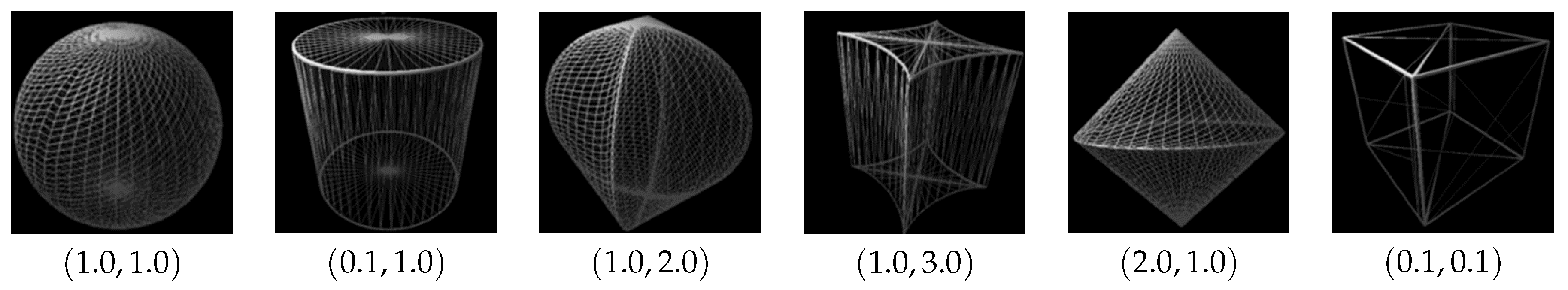
Superquadric functions are an extension of quadric surfaces and include supertoroids, superhyperboloids, and superellipsoids. Superellipsoids are most commonly used in object modeling because they define closed surfaces. Examples of elementary objects that can be represented with superellipsoids are depicted in Figure 2. Recently, superquadrics have been widely used for shape abstraction [24], object grasping [25,26], object localization [27], and object recognition [28].
A superquadric in an object-centered coordinate system can be defined by the inside–outside function with a scale parameter and a shape parameter :
where is a tuple as . Parameters , , and are scale parameters that define the superquadric size at the x, y, and z coordinates, respectively. The superquadric function F in Equation (1) with a unit scale can be re-written with the following parametric equation:
Parameters and are shape representation parameters that express squares along the z axis and the x-y plane. Given a point , if , the point is inside the superquadric, if , the point is outside the superquadric, and if the point lies on the surface of the superquadric. Further, the inside–outside description can be expressed in a generic coordinate system by adding six additional variables, representing the superquadric pose (three for translation and three Euler angles for rotation ), with a total of eleven independent variables, i.e., .
3. Methodology
The overview of our proposed method is illustrated in Figure 3. At the initial frame of the scene obtained from the depth sensor, such as Kinect, superquadric and pose parameters are estimated from segmented object 3D point cloud. At the successive frames, we do not estimate both superquadric parameters and pose parameters, but we only update pose parameters due to the instability of superquadric parameter estimation.
In Section 3.1 and Section 3.2, we apply both the initial and successive frames. In Section 3.3, we apply only the initial frame, and in Section 3.4 and Section 3.5, we apply only the successive frames.
3.1. Preprocessing
First, in the preprocessing stage, a depth map at current frame t is transformed into a metric vertex map , with the known camera intrinsic matrix , a depth map pixel in the image domain and its homogeneous representation . The vertex map is then smoothed by applying a median filter. The normal map of the current frame is simply generated from the vertex map by a cross-product of neighborhood pixels [29].
We assume that the z-axis of all the objects are horizontal to the normal vector of the floor plane at the initial depth frame . The preprocessing of plane estimation to the initial depth map is applied to extract the normal vector of the floor plane . We apply RANSAC-based plane parameter estimation to estimate the vector .
3.2. Geometric Segmentation
As primitive shapes have only convex surfaces, we segment the depth map into convex shapes. Tateno et al. [30] adapted the concave region penalty to the normal edge-based segmentation in their SLAM pipeline. We employ their segmentation approach. They classify each pixel irrespective of whether the pixel is an object edge by employing two operators. The first operator detects concave boundaries by computing the dot product between the normal vector of target pixel and each normal of the eight-connected neighboring pixels. The second operator takes into account the maximum 3D point-to-plane distance between the target pixel and its eight neighbors. In order to establish the threshold of the second operator, we employ an uncertainty measure computed following the noise model [31].
As a result, we obtain a binary geometric edge map at frame t, from the input depth frame. To the edge map , we apply a four-neighborhood connected component analysis algorithm to yield a label map , where each element is associated with a segment label . Unlike the method in [30], we do not segment the points on the floor plane to extract the object point cloud.
3.3. Superquadric Fitting
The i-th superquadric surface , which best represents the object, is estimated from given K 3D points of the i-th object’s 3D points cloud. The superquadric surface is represented by and . The minimization of the algebraic distance from points to the superquadric surface can be solved by defining a non-linear least-squares minimization problem:
where imposes the point to superquadric surface distance minimization, where the term is proportional to the superquadric volume, compensates for the fact that the previous equation is biased toward larger superquadric surfaces. is a rigid transformation by 6DoF pose . The Levenberg–Marquardt algorithm [32] is used to minimize the non-linear function Equation (3).
Moreover, Equation (3) is numerically unstable when and the superquadric surface has concavities with . We apply constraints when minimizing Equation (3) for shape parameters and for the scale parameters .
As the function in Equation (3) is not a convex function, the initial parameters determine on which local minimum the minimization converges. It is important to estimate the rough parameters: translation, rotation, scale, and shape parameters. First, as it is difficult to roughly estimate the shape of the object, the initial shape parameters and are set to 1, which implies that the shape of the initial model is an ellipsoid. Second, the centroid of all 3D data points can be used to estimate the initial translation. Third, to compute the initial rotation, we gauge the covariance matrix of all 3D data points. From this covariance matrix, we can compute three pairs of eigenvectors and eigenvalues. The largest eigenvector of the covariance matrix always points in the direction of the largest variance of the data, while the magnitude of this largest vector equals the corresponding eigenvalue. The second-largest eigenvector is always orthogonal to the largest and points in the direction of the second largest spread of the data, which is the same as the third vector. Therefore, the eigenvectors can be used as the initial rotation parameters, and the eigenvalues can be used as the initial scale parameters.
3.4. Label Matching
As the labels of the label maps and do not correspond to each other, labels between sequential frames must be matched. We re-label the label map using the overlapping area of two frames. We denote the number of pixels that satisfies the label of label map is and the label of label map is as . We normalize this term in the following manner:
where is the number of pixels with the label at label map . We re-label by finding the label at the , which maximizes :
If , we re-label the label at to .
3.5. Superquadric Tracking
As superquadric fitting is numerically unstable, we do not sequentially estimate parameters based on the assumption that the shape of the objects does not change sequentially. We only update the pose parameters at consecutive frames. The naive approach to estimate the pose at frame t is
where is the estimated superquadric parameters at the initial frame.
However, the outliers which are caused by miss-segmentation lead to the low accuracy of pose estimation. Therefore, we down-weigh the points that are far away from the center of objects during optimization by introducing a coefficient, .
A naive approach to down-weighing distant points is employing threshold value based on the Euclidean distance from the centroid of the object and each point. However, there can be two possible problems here. First, as the distance is defined in absolute scale, the threshold value might differ between different scaled objects. Second, calculating the distance in Euclidean Space is not compatible for a superquadric parameter estimation, because the distance in superquadric shape is non-linear. Therefore, we introduce a scale-invariant non-linear threshold parameter to down-weigh miss-segmented points for robust pose parameter estimation.
We introduce coefficient to the minimization equation, Equation (6), to eliminate the points distant from the origin in an object-centered coordinate system. First, we transform the point cloud by the transformation matrix at the previous frame. For a point defined by a vector in the transformed point cloud, there is a scalar value and vector on the superquadric surface, which satisfies . Thus, for vector , the following equation holds:
From this equation, it follows that
Instead of estimating the pose directly, we estimate the residual pose . Therefore, the equation below is applied to estimate the residual pose (using ):
We define the hyperparameter as throughout the experiment.
4. Experiments
4.1. Dataset
As there is no dataset that has a sequence in which the person moves primitive-shaped objects, we created the dataset using Kinect v.1 to evaluate our pose estimation method. In this paper, we did not conduct the evaluation using the synthetic dataset, because the effectiveness of the proposed method can only be validated using the data captured in the real environment. The main task of this paper is to robustly estimate the pose of primitive shaped objects in the case that the object point clouds cannot be accurately segmented. Although the sensor noise can be added to the acquired synthetic data, it is difficult to simulate the miss-segmentation.
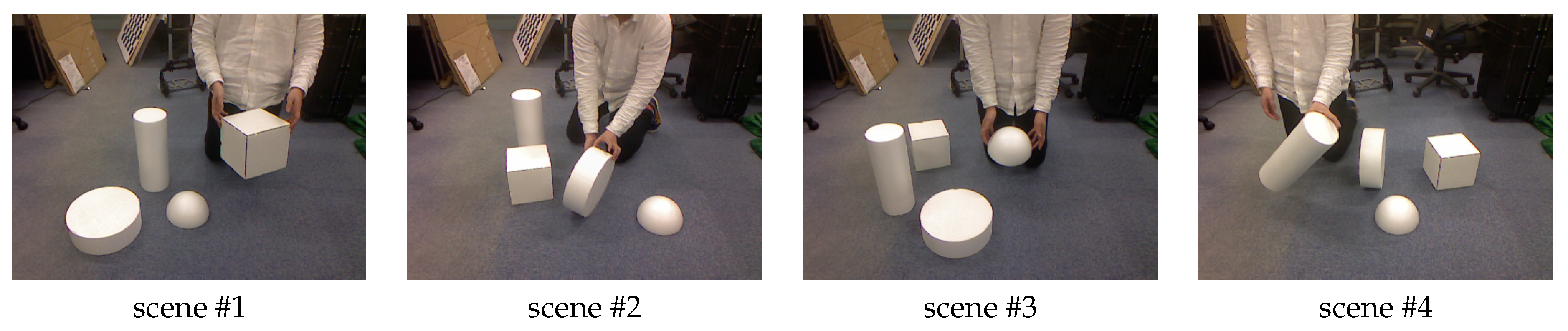
Four primitive-shaped objects were used in the experiments. The objects used in the experiment were cube (length = 20 cm), tall cylinder (radius = cm, height = 40 cm), wide cylinder (radius = 15 cm, height = 5 cm), and half sphere (radius = 10 cm). These objects are illustrated in Figure 4. In the dataset, there are 10 scenes included, and each scene comprised approximately 220 frames. At each scene, the user lifted, piled, and moved each object. The examples of frames in the scene are depicted in Figure 5.
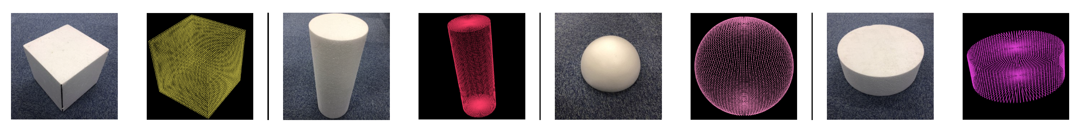
The ground truth pose is needed to evaluate our proposed method. We used Cloudcompare [33] to annotate the ground truth pose. First, the synthesized primitive-shaped objects are generated. The detailed explanation to generate the object point cloud is explained in the later section. For example, we set superquadric parameter for generating a cube, and for generating a tall cylinder. Third, we manually align the generated model to the point cloud of each frame. By extracting the transformation matrix after the alignment, we can obtain the ground truth pose of each primitive-shaped object.
4.2. Evaluation Metrics
We employed two metrics: 3D error and 2D error. 3D error measures the 3D Euclidean distance between point cloud transformed by ground truth 6DoF pose and by predicted pose. 2D error measures the 2D image pixel distance between the pixel in which the 3D point is projected onto the image using ground-truth pose and the predicted pose.
For the 3D error, we employed the 3D average distance metric for the symmetric object proposed by Hinterstoisser et al. [34]:
where x is a point sampled from object point cloud , is the ground truth pose, and is the predicted pose.
For the 2D error, we employed 2D projection metric (2D error) which is suited for applications such as a augmented reality [35]. An error is calculated as follows:
where is a camera intrinsic parameters which project the 3D points to the 2D image plane. Both metrics are that lower is better.
We sample M points from the superquadric surface to generate x. By sampling a point from a unit superquadric surface, according to Equation (2), the points that have a high curvature are emphasized. For an unbiased sample distribution, we need to apply equidistant rendering using spherical angles, as introduced by Bardinet et al. [36],
where,
The generated ground-truth models are visualized in Figure 4 right. Note that this model is only used to annotate the ground-truth pose and calculate the evaluation metrics.
4.3. The Comparison with Other Methods and the Baseline Method
In order to evaluate the effectiveness of our pose estimation, we compared the pose estimation accuracy with four methods. First, we compare with Iterative Closest Point (ICP) algorithm with point-to-plane metric [7], which achieves faster convergence than the point-to-point metric. Unlike the point-to-point metric, which has a closed-form solution, the point-to-plane metric is usually solved using the standard nonlinear least squares method, we employ the Levenberg–Marquardt algorithm. Second, we compare with feature-based RANSAC method, proposed by Buch et al. [37]. We employ Fast Point Feature Histograms (FPFH) feature extractor to extract the point features and match the features using RANSAC with pre-rejection step pose in the estimation loop in order to avoid verification of pose hypotheses that are likely to be wrong. Thirdly, we compare with Normal Distributions Transform (NDT) algorithm [38]. At last, we compare with our baseline method, which does not employ coefficient at Equation (9), to evaluate the effectiveness of excluding the outlier points implicitly.
Note that the baseline and our method estimates the shape, scale, and the pose of each object at the initial frame, and only the pose parameter is updated for the successive frames. For the other methods (ICP [7], NDT [38], RANSAC [37]), we estimate the pose between two successive frames using objects’ point cloud.
Sano et al. [16] also estimate the poses of a cube from a depth image, for instance. However, as the conventional methods for primitive shape pose estimation have to know the type of primitive shaped objects (e.g., cuboid, cylinder and sphere) before estimating the pose. Instead, we employ superquadrics to represent the primitive shapes so that the representative primitive shapes can be represented using a single equation. Moreover, the method proposed by Sano et al. [16] has an assumption that the two faces of the cuboid can be seen from the camera. As the fair comparison against these methods is difficult, we did not conduct the comparison against them.
5. Qualitative Evaluation
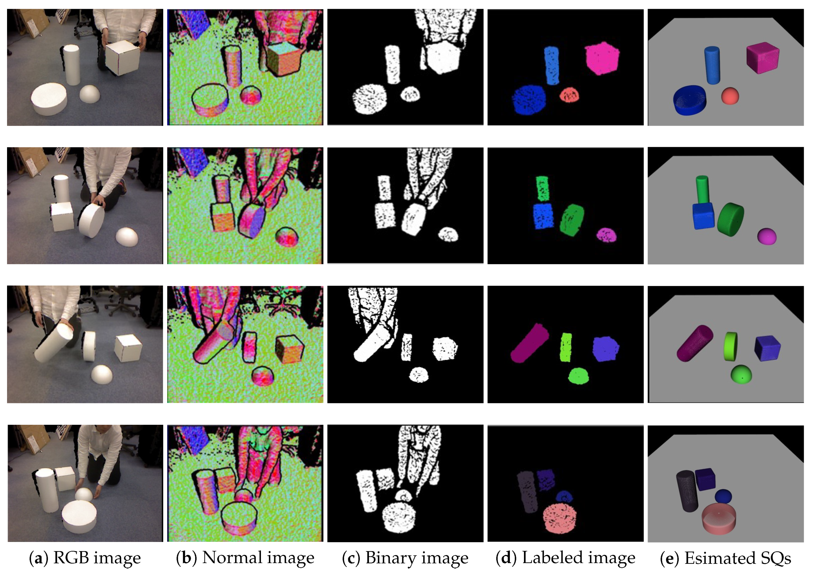
In this section, we evaluate the accuracy of the pose estimated by our approach. The qualitative results are illustrated in Figure 6. We present results of superquadric and pose parameter estimation from four scenes. The images in column Figure 6a depict RGB images of the scene, Figure 6b the visualized normal map, Figure 6c the binary segmented image (Section 3.2), Figure 6d the labeled image, and Figure 6e the visualized superquadric surface and ground plane (colored in grey). Note that the RGB images are shown just as the reference, and the pixels of the person are eliminated due to the label matching in Section 3.4. The figure confirms that the shape and the pose of each primitive-shaped object are estimated in different scenes. Moreover, it is evident that the pose of primitives can be successfully estimated even if the user touches and moves with the objects.
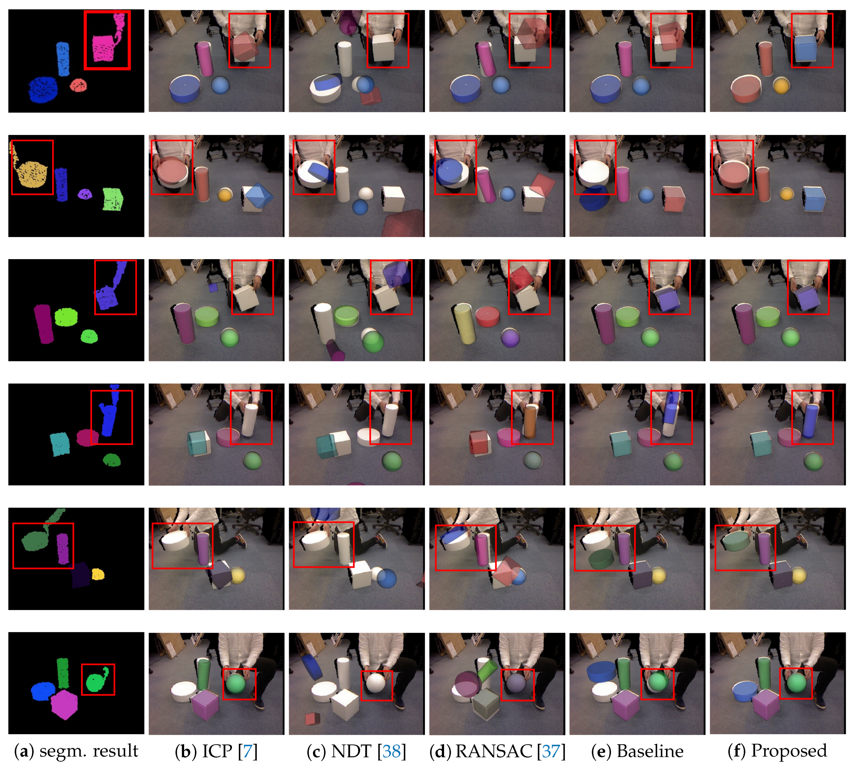
We compare the pose estimation results with three conventional methods and one baseline method. The qualitative results are shown in Figure 7. Note that the estimated superquadric surface is used to visualize the result of pose estimation. In these scenes, miss-segmentation was occurred due to the interaction with the user and the object (drew a rectangle in red). Although the pose estimation failed with the baseline and the conventional methods (Figure 7b–e), our proposed method successfully estimated the pose of each object (Figure 7f). As the geometric segmentation cannot distinguish the pixels of person and object, the pose estimation is conducted with an entire labeled pixel. This verifies the robustness of the proposed method against the miss-segmentation of object pixels.
6. Quantitative Evaluation
The quantitative results for each object are summarized in Table 1. We calculate the average error of the entire 10 scenes in our dataset and summarized per primitive-shaped object. We exclude the frames that failed to match the point cloud (Section 3.4) in order to purely compare the object pose estimation accuracy. It can be seen that the proposed method outperforms the conventional methods [7,37,38] and the baseline method for all of the objects. Even though the RANSAC-based method [37] outperformed the baseline for cylindrical objects, introducing the coefficient improves the performance.
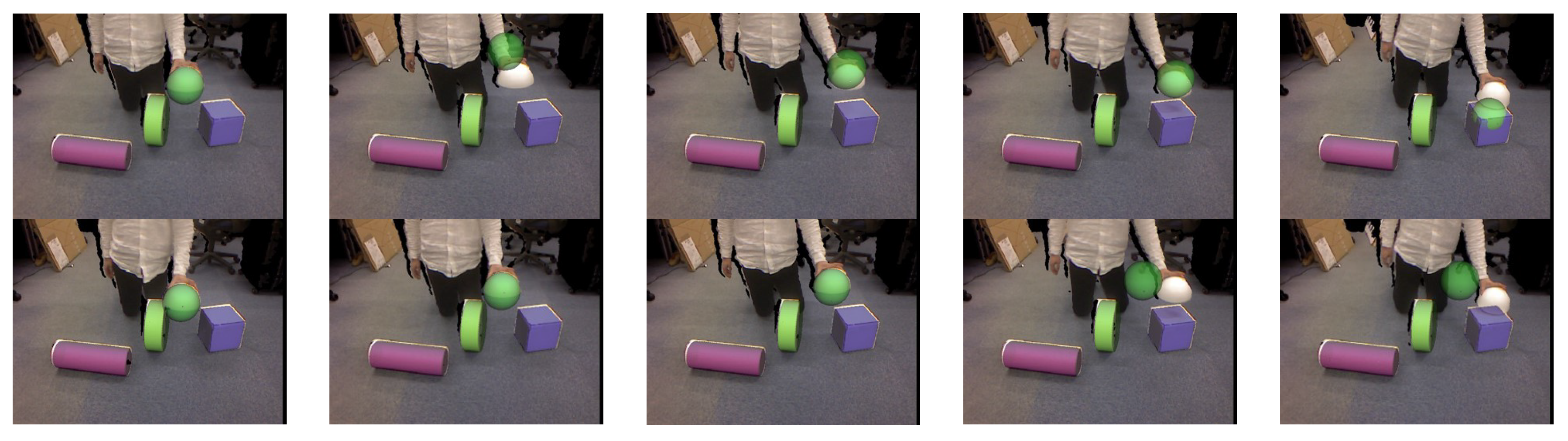
The quantitative results for each scene are summarized in Table 2. It can be seen that our method outperformed the conventional and baseline methods for most of the scenes. For the scenes in which the baseline outperforms the proposed method, our robust pose estimation method failed to track the objects. The example failure is visualized in Figure 8. As our method implicitly exclude the 3D points which are distant from the superquadric surface, the point clouds of fast-moving objects are not considered for pose estimation. In the bottom figure, the pose of the sphere was not updated due to the fast movement of the object.
7. Discussion
Currently, the proposed method cannot run at real-time speeds, but instead around 30 FPS. Although geometric segmentation and label matching can run at a reasonable frame rate (over 30FPS), pose estimation cannot. The computational time of the proposed method is summarized in Table 3. Note that the proposed system was implemented on a Windows 10 64-bit laptop with an Intel Core i7-6950X 3.00 GHz CPU, and 16 GB memory. We did not use any GPUs in the system. Further, we were able to confirm that the pose update process is crucial. Even if there is a single object in the scene, the pose update takes 97 ms and this is not in real-time.
To achieve the same results in a real-time system, we can employ the fast parameter estimation method proposed by Duncan et al. [39]. They proposed a method to estimate the superquadric parameters in near real-time. They down-sampled the input point cloud recursively until the optimization failed. Although they achieved 40 ms, this is not still suitable for augmented reality or a robot grasping system. Another solution is implementing the Levenberg–Marquardt algorithm using GPU [40]. Currently, as our system does not use any GPU acceleration, it can be expected to estimate parameters in real-time.
In this paper, three types of primitive shapes (cuboid, sphere, and cylinder) and four objects were used to construct the dataset. Even though the types of primitive shaped objects are limited, the dataset includes the representative primitive shapes that are used in the conventional primitive shape estimation methods [16,19]. Also, unlike existing methods, our method uses superquadrics for the primitive shape representation, which enables us to estimate the shape and the pose regardless of the type of the primitive shape (sphere, cylinder, cuboid, etc.). Although only four objects were used in the experiments, Figure 6 and Figure 7 show that the superquadrics (shape and scale) parameters were correctly estimated. As the shape and scale parameters are estimated at the initial frame, our method can be extended to other primitive shaped objects as long as the objects can be represented by superquadrics. The purpose of this paper is not object shape classification, so we did not conduct experiments with a variety of primitive shaped objects, but this can be an important subject for future study.
8. Conclusions
In this paper, we proposed a method for estimating the six Degrees of Freedom (6DoF) pose of texture-less primitive-shaped objects from a depth image. The method is robust to outliers, which are caused by the miss-segmentation of the depth image. To achieve robustness, we introduced the novel pose estimation method. We implicitly ignore the points that are distant from the object point cloud to ensure that the optimization is conducted with the only object’s point cloud. Further, we generated a new data set in the experiments. In this dataset, the user interactively moves the primitive-shaped objects. The experimental results revealed the effectiveness of our novel estimation method by comparing the pose accuracy for primitive shaped objects.
There are several future works that can be considered. First, as mentioned in the discussion section, we aim to achieve real-time computation of superquadric parameters. Second, currently, out pose estimation method relies on the preprocessing steps, such as geometric segmentation and segment matching, of the obtained depth image to extract the object point cloud. However, the pose of the objects cannot be estimated if these preprocessing steps failed to extract the point cloud of the target object. We will further investigate the method to estimate the pose of the objects from the raw depth image.
Author Contributions
Data curation, R.H.; Funding acquisition, H.S.; Methodology, R.H.; Software, R.H.; Supervision, H.S.; Validation, R.H.; Visualization, R.H.; Writing—original draft, R.H.; Writing—review and editing, H.S. All authors have read and agreed to the published version of the manuscript.
Funding
This work was enabled by the Japan Science and Technology Agency (JST) under grant CREST-JPMJCR1683.
Conflicts of Interest
The authors declare no conflict of interest.
References
- Rad, M.; Lepetit, V. BB8: A Scalable, Accurate, Robust to Partial Occlusion Method for Predicting the 3D Poses of Challenging Objects without Using Depth. In Proceedings of the 2017 IEEE International Conference on Computer Vision (ICCV), Venice, Italy, 22–29 October 2017; pp. 3848–3856. [Google Scholar] [CrossRef] [Green Version]
- Sundermeyer, M.; Marton, Z.C.; Durner, M.; Brucker, M.; Triebel, R. Implicit 3D Orientation Learning for 6D Object Detection from RGB Images. In Proceedings of the European Conference on Computer Vision (ECCV) 2018, Munich, Germany, 8–14 September 2018. [Google Scholar]
- Peng, S.; Liu, Y.; Huang, Q.; Zhou, X.; Bao, H. PVNet: Pixel-wise Voting Network for 6DoF Pose Estimation. In Proceedings of the CVPR 2019, Long Beach, CA, USA, 15–21 June 2019. [Google Scholar]
- Rusu, R.B.; Blodow, N.; Beetz, M. Fast Point Feature Histograms (FPFH) for 3D registration. In Proceedings of the 2009 IEEE International Conference on Robotics and Automation, Kobe, Japan, 12–17 May 2009; pp. 3212–3217. [Google Scholar] [CrossRef]
- Drost, B.; Ulrich, M.; Navab, N.; Ilic, S. Model globally, match locally: Efficient and robust 3D object recognition. In Proceedings of the 2010 IEEE Computer Society Conference on Computer Vision and Pattern Recognition, San Francisco, CA, USA, 13–18 June 2010; pp. 998–1005. [Google Scholar] [CrossRef] [Green Version]
- Wang, H.; Sridhar, S.; Huang, J.; Valentin, J.; Song, S.; Guibas, L.J. Normalized Object Coordinate Space for Category-Level 6D Object Pose and Size Estimation. In Proceedings of the IEEE Conference on Computer Vision and Pattern Recognition 2019, Long Beach, CA, USA, 15–21 June 2019. [Google Scholar]
- Chen, Y.; Medioni, G. Object modeling by registration of multiple range images. In Proceedings of the 1991 IEEE International Conference on Robotics and Automation, Sacramento, CA, USA, 9–11 April 1991; Volume 3, pp. 2724–2729. [Google Scholar] [CrossRef]
- Rünz, M.; Agapito, L. Co-Fusion: Real-time Segmentation, Tracking and Fusion of Multiple Objects. In Proceedings of the 2017 IEEE International Conference on Robotics and Automation (ICRA), Las Vegas, NV, USA, 29 May–3 June 2017; pp. 4471–4478. [Google Scholar]
- Runz, M.; Buffier, M.; Agapito, L. MaskFusion: Real-Time Recognition, Tracking and Reconstruction of Multiple Moving Objects. In Proceedings of the 2018 IEEE International Symposium on Mixed and Augmented Reality (ISMAR), Munich, Germany, 16–20 October 2018; pp. 10–20. [Google Scholar] [CrossRef] [Green Version]
- Fischler, M.A.; Bolles, R.C. Random Sample Consensus: A Paradigm for Model Fitting with Applications to Image Analysis and Automated Cartography. Commun. ACM 1981, 24, 381–395. [Google Scholar] [CrossRef]
- Tombari, F.; Di Stefano, L. Hough Voting for 3D Object Recognition under Occlusion and Clutter. IPSJ Trans. Comput. Vis. Appl. 2012, 4. [Google Scholar] [CrossRef] [Green Version]
- Barr, A.H. Superquadrics and angle-preserving transformations. IEEE Comput. Graph. Appl. 1981, 1, 11–23. [Google Scholar] [CrossRef] [Green Version]
- Solina, F.; Bajcsy, R. Range image interpretation of mail pieces with superquadrics. In Proceedings of the 6th National Conference on Artificial Intelligence, Seattle, WA, USA, 13–17 July 1987; pp. 733–737. [Google Scholar]
- Xiang, Y.; Schmidt, T.; Narayanan, V.; Fox, D. PoseCNN: A Convolutional Neural Network for 6D Object Pose Estimation in Cluttered Scenes. arXiv 2018, arXiv:1711.00199. [Google Scholar]
- Birdal, T.; Ilic, S. Point Pair Features Based Object Detection and Pose Estimation Revisited. In Proceedings of the 2015 International Conference on 3D Vision, Lyon, France, 19–22 October 2015; pp. 527–535. [Google Scholar] [CrossRef]
- Sano, M.; Matsumoto, K.; Thomas, B.H.; Saito, H. [POSTER] Rubix: Dynamic Spatial Augmented Reality by Extraction of Plane Regions with a RGB-D Camera. In Proceedings of the 2015 IEEE International Symposium on Mixed and Augmented Reality, Yucatan, Mexico, 19–23 September 2016; pp. 148–151. [Google Scholar] [CrossRef]
- Hachiuma, R.; Saito, H. Recognition and pose estimation of primitive shapes from depth images for spatial augmented reality. In Proceedings of the 2016 IEEE 2nd Workshop on Everyday Virtual Reality (WEVR), Greenville, SC, USA, 20 March 2016; pp. 32–35. [Google Scholar] [CrossRef]
- Buttner, S.; Marton, Z.C.; Hertkorn, K. Automatic scene parsing for generic object descriptions using shape primitives. Robot. Auton. Syst. 2016, 76, 93–112. [Google Scholar] [CrossRef]
- Stanescu, A.; Fleck, P.; Schmalstieg, D.; Arth, C. Semantic Segmentation of Geometric Primitives in Dense 3D Point Clouds. In Proceedings of the 2018 IEEE International Symposium on Mixed and Augmented Reality Adjunct (ISMAR-Adjunct), Munich, Germany, 16–20 October 2018; pp. 206–211. [Google Scholar] [CrossRef]
- Somani, N.; Cai, C.; Perzylo, A.; Rickert, M.; Knoll, A. Object Recognition Using Constraints from Primitive Shape Matching. In Advances in Visual Computing; Bebis, G., Boyle, R., Parvin, B., Koracin, D., McMahan, R., Jerald, J., Zhang, H., Drucker, S.M., Kambhamettu, C., El Choubassi, M., et al., Eds.; Springer International Publishing: Cham, Switzerland, 2014; pp. 783–792. [Google Scholar]
- Tran, T.T.; Cao, V.T.; Laurendeau, D. Extraction of cylinders and estimation of their parameters from point clouds. Comput. Graph. 2015, 46, 345–357. [Google Scholar] [CrossRef]
- Drost, B.; Ilic, S. Local Hough Transform for 3D Primitive Detection. In Proceedings of the 2015 International Conference on 3D Vision, Lyon, France, 19–22 October 2015; pp. 398–406. [Google Scholar] [CrossRef]
- Holz, D.; Holzer, S.; Rusu, R.B.; Behnke, S. Real-Time Plane Segmentation Using RGB-D Cameras; Röfer, T., Mayer, N.M., Savage, J., Saranlı, U., Eds.; Springer: Berlin, Germany, 2012; pp. 306–317. [Google Scholar]
- Paschalidou, D.; Ulusoy, A.O.; Geiger, A. Superquadrics Revisited: Learning 3D Shape Parsing beyond Cuboids. In Proceedings of the IEEE Conference on Computer Vision and Pattern Recognition 2019, Long Beach, CA, USA, 15–21 June 2019. [Google Scholar]
- Vezzani, G.; Pattacini, U.; Natale, L. A grasping approach based on superquadric models. In Proceedings of the 2017 IEEE International Conference on Robotics and Automation (ICRA), Las Vegas, NV, USA, 29 May–3 June 2017; pp. 1579–1586. [Google Scholar] [CrossRef]
- Makhal, A.; Thomas, F.; Gracia, A.P. Grasping Unknown Objects in Clutter by Superquadric Representation. In Proceedings of the 2018 Second IEEE International Conference on Robotic Computing (IRC), Laguna Hills, CA, USA, 31 January–2 February 2018; pp. 292–299. [Google Scholar] [CrossRef] [Green Version]
- Vaskevicius, N.; Pathak, K.; Birk, A. Fitting superquadrics in noisy, partial views from a low-cost RGBD sensor for recognition and localization of sacks in autonomous unloading of shipping containers. In Proceedings of the 2014 IEEE International Conference on Automation Science and Engineering (CASE), Taipei, Taiwan, 18–22 August 2014; pp. 255–262. [Google Scholar] [CrossRef]
- Hachiuma, R.; Ozasa, Y.; Saito, H. Primitive Shape Recognition via Superquadric Representation using Large Margin Nearest Neighbor Classifier. In Proceedings of the 12th International Joint Conference on Computer Vision, Imaging and Computer Graphics Theory and Applications, Porto, Portugal, 27 February–1 March 2017; pp. 325–332. [Google Scholar] [CrossRef] [Green Version]
- Holzer, S.; Rusu, R.B.; Dixon, M.; Gedikli, S.; Navab, N. Adaptive neighborhood selection for real-time surface normal estimation from organized point cloud data using integral images. In Proceedings of the 2012 IEEE/RSJ International Conference on Intelligent Robots and Systems, Algarve, Portugal, 7–12 October 2012; pp. 2684–2689. [Google Scholar] [CrossRef]
- Tateno, K.; Tombari, F.; Navab, N. Real-time and scalable incremental segmentation on dense SLAM. In Proceedings of the 2015 IEEE/RSJ International Conference on Intelligent Robots and Systems (IROS), Hamburg, Germany, 28 September–2 October 2015; pp. 4465–4472. [Google Scholar] [CrossRef]
- Nguyen, C.V.; Izadi, S.; Lovell, D. Modeling Kinect Sensor Noise for Improved 3D Reconstruction and Tracking. In Proceedings of the 2012 Second International Conference on 3D Imaging, Modeling, Processing, Visualization Transmission, Zurich, Switzerland, 13–15 October 2012; pp. 524–530. [Google Scholar] [CrossRef]
- Moré, J.J. The Levenberg-Marquardt algorithm: Implementation and theory. In Numerical Analysis; Springer: Berlin, Germany, 1978; pp. 105–116. [Google Scholar]
- Girardeau-Montaut, D. CloudCompare. Available online: https://www.danielgm.net/cc/ (accessed on 8 May 2020).
- Hinterstoisser, S.; Lepetit, V.; Ilic, S.; Holzer, S.; Bradski, G.; Konolige, K.; Navab, N. Model Based Training, Detection and Pose Estimation of Texture-Less 3D Objects in Heavily Cluttered Scenes; Lee, K.M., Matsushita, Y., Rehg, J.M., Hu, Z., Eds.; Springer: Berlin, Germany, 2013; pp. 548–562. [Google Scholar]
- Brachmann, E.; Michel, F.; Krull, A.; Yang, M.Y.; Gumhold, S.; Rother, C. Uncertainty-Driven 6D Pose Estimation of Objects and Scenes from a Single RGB Image. In Proceedings of the 2016 IEEE Conference on Computer Vision and Pattern Recognition (CVPR), Las Vegas, NV, USA, 26 June 26–1 July 2016; pp. 3364–3372. [Google Scholar]
- Bierbaum, A.; Gubarev, I.; Dillmann, R. Robust shape recovery for sparse contact location and normal data from haptic exploration. In Proceedings of the 2008 IEEE/RSJ International Conference on Intelligent Robots and Systems, Nice, France, 22–26 September 2008; pp. 3200–3205. [Google Scholar] [CrossRef]
- Buch, A.G.; Kraft, D.; Kamarainen, J.; Petersen, H.G.; Krüger, N. Pose estimation using local structure-specific shape and appearance context. In Proceedings of the 2013 IEEE International Conference on Robotics and Automation, Karlsruhe, Germany, 6–10 May 2013; pp. 2080–2087. [Google Scholar]
- Magnusson, M. The Three-Dimensional Normal-Distributions Transform—An Efficient Representation for Registration, Surface Analysis, and Loop Detection. Ph.D. Thesis, Örebro University, Örebro, Sweden, 2009. [Google Scholar]
- Duncan, K.; Sarkar, S.; Alqasemi, R.; Dubey, R. Multi-scale superquadric fitting for efficient shape and pose recovery of unknown objects. In Proceedings of the 2013 IEEE International Conference on Robotics and Automation, Karlsruhe, Germany, 6–10 May 2013; pp. 4238–4243. [Google Scholar] [CrossRef]
- Przybylski, A.; Thiel, B.; Keller-Findeisen, J.; Stock, B.; Bates, M. Gpufit: An open-source toolkit for GPU-accelerated curve fitting. Sci. Rep. 2017, 7, 15722. [Google Scholar] [CrossRef] [Green Version]
Figure 1.
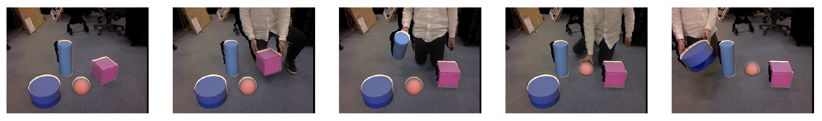
Our method estimates the shape, size, and the pose of the primitive shaped objects in the scene and the detected objects are tracked sequentially. The results of pose estimation is overlaid onto the RGB image for the visualization, and we do not use any color information, but only use the depth images.
Figure 1.
Our method estimates the shape, size, and the pose of the primitive shaped objects in the scene and the detected objects are tracked sequentially. The results of pose estimation is overlaid onto the RGB image for the visualization, and we do not use any color information, but only use the depth images.

Figure 2.
Various superquadric shapes according to and The caption below the figure shows the .

Figure 3.
An overview of our proposed method.

Figure 4.
Primitive-shaped objects used in the experiment (left) and the generated point clouds (right) for each object. From left to right, cuboid, tall cylinder, sphere, and wide cylinder. The generated point clouds are used just as the evaluation and annotation of ground-truth pose.
Figure 4.
Primitive-shaped objects used in the experiment (left) and the generated point clouds (right) for each object. From left to right, cuboid, tall cylinder, sphere, and wide cylinder. The generated point clouds are used just as the evaluation and annotation of ground-truth pose.

Figure 5.
Examples of frames included in the dataset.

Figure 6.
Output images of the each processing step at different scenes. (a) RGB image of the captured scene, (b) normal map, (c) geometric segmentation result, (d) labeling result, and (e) superquadric and pose parameter estimation result. Superquadric surfaces were rendered onto 2D images.
Figure 6.
Output images of the each processing step at different scenes. (a) RGB image of the captured scene, (b) normal map, (c) geometric segmentation result, (d) labeling result, and (e) superquadric and pose parameter estimation result. Superquadric surfaces were rendered onto 2D images.

Figure 7.
Comparison of the pose estimation results. (a) geometric segmentation result, pose estimation result by (b) Iterative Closest Point (ICP) tracking, (c) Normal Distributions Transform (NDT) algorithm, (d) RANSAC-based feature matching method, (e) the baseline method, and (f) the proposed method. Superquadric surfaces were rendered onto a 2D image.

Figure 8.
The failure of the proposed method. The upper row shows the results of the baseline method and the bottom row shows the results of the proposed method. The column shows the five successive frames in the scene.
Figure 8.
The failure of the proposed method. The upper row shows the results of the baseline method and the bottom row shows the results of the proposed method. The column shows the five successive frames in the scene.


Table 1.
Error of primitive shape pose estimation (per object). It is evident that our proposed method outperforms the baseline and the other methods.
Table 1.
Error of primitive shape pose estimation (per object). It is evident that our proposed method outperforms the baseline and the other methods.
| 3D Error [cm] ↓ | |||||
| Object | ICP [7] | NDT [38] | RANSAC [37] | Baseline | Ours |
| Sphere | 4.213 | 8.645 | 0.642 | 0.072 | 0.070 |
| Tall cylinder | 3.194 | 193.7 | 2.001 | 2.738 | 0.502 |
| Wide cylinder | 2.104 | 28.65 | 2.013 | 2.140 | 0.808 |
| Cube | 5.212 | 41.46 | 1.829 | 0.867 | 0.420 |
| 2D Error [px]↓ | |||||
| Object | ICP [7] | NDT [38] | RANSAC [37] | Baseline | Ours |
| Sphere | 24.03 | 44.81 | 14.50 | 4.232 | 4.012 |
| Tall cylinder | 19.52 | 45.76 | 15.46 | 29.78 | 7.418 |
| Wide cylinder | 11.83 | 71.25 | 19.97 | 31.26 | 3.478 |
| Cube | 24.52 | 72.59 | 27.10 | 7.423 | 5.010 |
Table 2.
Error of primitive shape pose estimation (per scene) using our dataset. S1 to S10 denotes the indices of the scene in the dataset. The rightmost column shows the average of entire scenes.
Table 2.
Error of primitive shape pose estimation (per scene) using our dataset. S1 to S10 denotes the indices of the scene in the dataset. The rightmost column shows the average of entire scenes.
| 3D Error [cm] ↓ | |||||||||||
| Method | S1 | S2 | S3 | S4 | S5 | S6 | S7 | S8 | S9 | S10 | Ave. |
| ICP [7] | 0.080 | 5.012 | 1.723 | 1.409 | 1.382 | 5.887 | 5.964 | 1.392 | 6.935 | 6.919 | 3.670 |
| NDT [38] | 37.52 | 70.77 | 52.23 | 62.04 | 73.35 | 64.01 | 60.28 | 112.4 | 97.52 | 95.24 | 72.53 |
| RANSAC [37] | 0.714 | 2.145 | 3.077 | 0.184 | 0.785 | 4.335 | 0.362 | 1.201 | 1.720 | 1.524 | 1.604 |
| Baseline | 0.096 | 0.230 | 5.800 | 0.197 | 0.245 | 4.232 | 1.113 | 0.015 | 0.064 | 0.010 | 1.200 |
| Ours | 0.052 | 0.695 | 1.135 | 1.342 | 0.268 | 0.995 | 0.007 | 0.003 | 0.015 | 0.010 | 0.452 |
| 2D Error [px]↓ | |||||||||||
| Method | S1 | S2 | S3 | S4 | S5 | S6 | S7 | S8 | S9 | S10 | Ave. |
| ICP [7] | 3.378 | 67.10 | 8.973 | 5.301 | 1.204 | 33.25 | 33.25 | 1.562 | 21.32 | 24.53 | 19.98 |
| NDT [38] | 149.8 | 19.12 | 56.44 | 18.10 | 34.57 | 65.65 | 133.1 | 32.42 | 25.31 | 53.21 | 58.78 |
| RANSAC [37] | 9.816 | 27.54 | 19.60 | 18.72 | 15.23 | 28.42 | 11.48 | 21.53 | 23.52 | 12.52 | 18.83 |
| Baseline | 3.280 | 3.447 | 43.26 | 5.724 | 4.678 | 23.62 | 15.76 | 1.780 | 3.594 | 2.130 | 10.73 |
| Ours | 2.152 | 2.803 | 4.609 | 17.23 | 6.452 | 13.63 | 1.670 | 1.381 | 16.10 | 2.059 | 6.809 |
Table 3.
Computational time of the each step (ms). Note that the pose of objects is estimated independently, and the overall system takes a time to run if a large number of objects exist in the scene.
Table 3.
Computational time of the each step (ms). Note that the pose of objects is estimated independently, and the overall system takes a time to run if a large number of objects exist in the scene.
| Process | Segmentation | Matching | Pose Update |
|---|---|---|---|
| Time (ms) | 20.4 | 13.4 | 97.2 per object |
© 2020 by the authors. Licensee MDPI, Basel, Switzerland. This article is an open access article distributed under the terms and conditions of the Creative Commons Attribution (CC BY) license (http://creativecommons.org/licenses/by/4.0/).
Share and Cite
MDPI and ACS Style
Hachiuma, R.; Saito, H. Pose Estimation of Primitive-Shaped Objects from a Depth Image Using Superquadric Representation. Appl. Sci. 2020, 10, 5442. https://doi.org/10.3390/app10165442
AMA Style
Hachiuma R, Saito H. Pose Estimation of Primitive-Shaped Objects from a Depth Image Using Superquadric Representation. Applied Sciences. 2020; 10(16):5442. https://doi.org/10.3390/app10165442
Chicago/Turabian StyleHachiuma, Ryo, and Hideo Saito. 2020. "Pose Estimation of Primitive-Shaped Objects from a Depth Image Using Superquadric Representation" Applied Sciences 10, no. 16: 5442. https://doi.org/10.3390/app10165442
Note that from the first issue of 2016, this journal uses article numbers instead of page numbers. See further details here.