Characterizing Subsurface Rectangular Tilted Heat Sources Using Inductive Thermography

Featured Application

Thermographic nondestructive testing methods such as ultrasonically- and inductively-excited infrared thermography reveal defects by conversion of the input energy into heat at the flaws. This work shows that it is possible to characterize the size, depth, and inclination of inner heat sources from the measurement of the surface temperature. The results have straightforward application in the characterization of tilted flaws producing heat excited by above-mentioned thermographic testing methods.

Abstract

In this study, we characterize the lateral dimension, depth, and inclination of buried tilted rectangular heat sources from time domain temperature data measured at the surface. The heat sources are representative for planar defects that emit heat in thermographic tests with internal burst excitation. We present a semi-analytical expression for the evolution of the surface temperature distribution. The emitted flux, dimensions and inclination of the heat source are determined by fitting the model to two perpendicular surface temperature profiles and the temperature history at one point of the surface. We show that the sensitivity of the data to the geometrical parameters of the heat source decreases as the angle it makes with the surface increases. The study also shows that the optimum duration of the excitation corresponds to a thermal diffusion length covering the distance from the surface to the deepest end of the heat source. The accuracy and precision of the results for different noise levels and inclinations have been tested by fitting the model to synthetic data with added noise. Fittings of experimental induction thermography data on 3D printed photo-polymeric resin samples containing calibrated Cu slabs confirm that it is possible to characterize tilted rectangular heat sources from surface temperature data.

1. Introduction

Thermographic techniques have proven to be very efficient nondestructive testing methods for the detection of defects in a wide variety of materials [1]. They use infrared (IR) video-cameras to detect anomalies caused by flaws in the surface temperature distribution of a material after some kind of excitation. Optical excitation is the most common method used to induce a heat flux within a sample. In opaque materials, the optical energy absorbed at the surface produces a temperature elevation and a subsequent heat flow. The presence of a defect distorts heat diffusion and produces an anomaly in the surface temperature distribution that is measured with an IR camera. Therefore, the presence of the flaw represents just a perturbation of an existing temperature field. On the contrary, in other thermographic modalities with ultrasonic [2] or inductive excitation [3] (vibrothermography and inductive thermography, respectively), heat is mainly generated at the defects. In the case of cracks or delaminations excited with ultrasounds, the main mechanism for heat production is the friction between the asperities of the moving faces of the defect under ultrasonic vibration [4], which turns the flaw into a heat source in a cold environment. The defect is detected as a temperature elevation at the surface, above the defect. In consequence, the technique is defect-selective, as the (excess) temperature field in the specimen is only due to the presence of the defect. Similarly, the detection of electrically conducting inclusions within isolating materials by inductive heating of the foreign material makes the inclusion behave as a heat source in a cold environment. However, the most common application of inductive thermography is the detection of cracks in electrically conducting parts [3]. In these applications, Eddy currents induced in the material generate heat by the Joule effect and the presence of cracks may distort either heat propagation or Eddy currents distribution, which often entails an additional source of heat.

The ultimate goal of nondestructive techniques is the characterization of defects, i.e., determination of size, location, and orientation. In the case of cracks excited by ultrasounds and foreign metallic inclusions embedded in electrical insulators excited inductively, the physical magnitude that can be characterized is the heat flux generated at the defect: dimensions of active area, location, orientation, and absolute values of the flux distribution. In the last decade, many efforts have been devoted to the characterization of planar heat sources perpendicular to the surface of the material, representing vertical fatigue cracks excited with ultrasounds [5,6,7,8,9,10,11,12]. For a broad overview, see [13]. In these works, the spatial extension and depth of vertical cracks was retrieved by inverting lock-in surface temperature data obtained under modulated excitation [5,6,7], as well as time domain data obtained under burst excitation [8,9,10]. In the latter modality, quantitative values of the local heat flux were determined locally along the crack surface [11,12]. Some authors have focused on the evaluation of the crack length using minimization algorithms [14] or image processing methods [15]. Recently, the virtual wave concept has been applied to the identification of volumetric heat sources generated inductively by metallic balls embedded in epoxy [16].

The works mentioned above are mostly addressed at characterizing vertical heat sources typically generated by fatigue cracks in ultrasound-excited thermography. However, cracks may feature any (unknown) inclination with respect to the sample surface. Very few works have addressed the problem of tilted heat sources in thermographic experiments. The virtual wave concept approach has been applied to determine the orientation of planar heat sources but not the size or emitted flux [17]. The influence of the crack inclination has also been analyzed in inductive thermography experiments in metallic samples [18]. In this work, we address the full characterization of planar heat sources with an arbitrary inclination with respect to the surface of the material, in time domain. For the first study, we focus on a particular geometry, rectangular heat sources, for which we determine the lateral dimensions, depth, inclination and emitted power density. In Section 2, we present a semi-analytical expression for the surface temperature distribution produced by a rectangular heat source of any inclination, and we illustrate the effect of the inclination on the surface temperature distribution. We propose to fit the model to two perpendicular temperature profiles and the temperature history at one position of the surface to characterize the heat source. In Section 3, we present a sensitivity analysis aimed at determining the optimum experimental conditions to carry out the characterization. In order to test the accuracy of the retrieved parameters as a function of the noise level in the data, in Section 4, we present fittings of the semi-analytical model to synthetic surface temperature data with added noise. In Section 5, we present experimental data taken with an inductive thermography set-up on samples containing calibrated metallic slabs with different orientations embedded in an IR opaque resin. The results prove that it is possible to determine the dimensions, depth, and inclination of the heat source from surface temperature data.

2. Theory

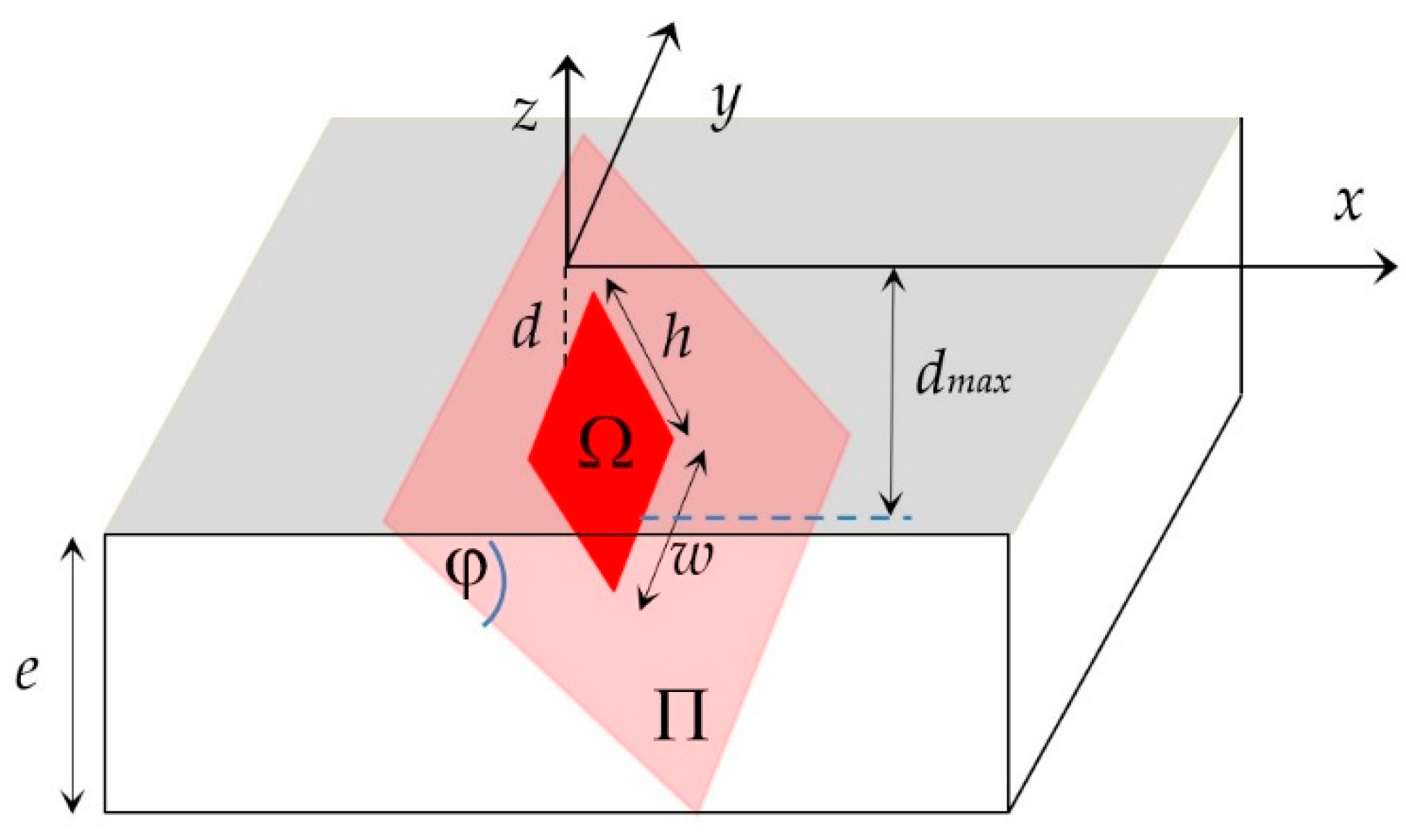
We calculate in this section the evolution of the surface temperature distribution produced by a rectangular heat source of area Ω in a plane Π having an angle φ with the surface. We consider that the rectangle emits a homogeneous power density (flux) Φ that is constant during a given time interval [0,τ] that we call burst. The rectangle has a width w, parallel to the surface where the temperature is measured. The height of the rectangle is h and the depth of the shallowest side is d. The maximum depth of the heat source is d_max = d + h sinφ. The geometry of the problem is depicted in Figure 1.

We start the calculation considering an instantaneous point-like heat source located at position $\overrightarrow{r}\prime$ that emits an energy H at a time t’ in an infinite homogeneous and isotropic medium of thermal conductivity and diffusivity K and D, respectively. The temperature elevation above the ambient at any point $\overrightarrow{r}$ and time t > t′ is given by the Green function [19]:

$$T(\overrightarrow{r},t)=\frac{HD}{8K{[\pi D(t-t\prime )]}^{3/2}}{e}^{-\frac{{|\overrightarrow{r}-\overrightarrow{r}\prime |}^2}{4D(t-t\prime )}}$$

(1)

We consider now that the point-like heat source emits a burst of constant power P during a time interval [0,τ]. The temperature elevation at any point in the infinite material can be calculated by integrating Equation (1) [19]:

$$T(\overrightarrow{r},t)=\frac{P}{4\pi K|\overrightarrow{r}-\overrightarrow{r}\prime |}Erfc\left[\frac{|\overrightarrow{r}-\overrightarrow{r}\prime |}{\sqrt{4Dt}}\right],0\le t\le \tau ,$$

(2)

$$T(\overrightarrow{r},t)=\frac{P}{4\pi K|\overrightarrow{r}-\overrightarrow{r}\prime |}\left\{Erfc\left[\frac{|\overrightarrow{r}-\overrightarrow{r}\prime |}{\sqrt{4Dt}}\right]-Erfc\left[\frac{|\overrightarrow{r}-\overrightarrow{r}\prime |}{\sqrt{4D(t-\tau )}}\right]\right\},\tau <t$$

(3)

where Erfc is the complementary error function.

In the next step, we take into account the spatial extension Ω of the heat source. The temperature at any position and time can be calculated by integrating the contribution of point-like heat sources of an infinitesimal area ds’ within the region Ω, with an eventually position dependent flux $\Phi (\overrightarrow{r}\prime )$ $\Phi (\overrightarrow{r})$:

$$T(\overrightarrow{r},t)={{\displaystyle \iint }}_{\Omega }\frac{\Phi ({\overrightarrow{r}}^{\prime })}{4\pi K|\overrightarrow{r}-\overrightarrow{r}\prime |}Erfc\left[\frac{|\overrightarrow{r}-\overrightarrow{r}\prime |}{\sqrt{4Dt}}\right]d{s}^{\prime },0\le t\le \tau ,$$

(4)

$$T(\overrightarrow{r},t)={{\displaystyle \iint }}_{\Omega }\frac{\Phi ({\overrightarrow{r}}^{\prime })}{4\pi K|\overrightarrow{r}-\overrightarrow{r}\prime |}\left\{Erfc\left[\frac{|\overrightarrow{r}-\overrightarrow{r}\prime |}{\sqrt{4Dt}}\right]-Erfc\left[\frac{|\overrightarrow{r}-\overrightarrow{r}\prime |}{\sqrt{4D(t-\tau )}}\right]\right\}d{s}^{\prime },\tau <t.$$

(5)

Finally, we consider that the material is an infinite plate in the directions x and y but has a given thickness e in the z direction. The surface where data are collected is located in plane z = 0 (see Figure 1). If heat losses by convection and radiation can be neglected, the effect of the sample surfaces can be taken into account by applying the images method, i.e., considering the effect of reflected images of the heat source at the front and back surfaces. The temperature elevation in the material is given by:

$$T(\overrightarrow{r},t)={{\displaystyle \iint }}_{\Omega +{\Omega }^{\prime }+{\Omega }^{″}+{\Omega }^{‴}+\dots }\frac{\Phi ({\overrightarrow{r}}^{\prime })}{4\pi K|\overrightarrow{r}-\overrightarrow{r}\prime |}Erfc\left[\frac{|\overrightarrow{r}-\overrightarrow{r}\prime |}{\sqrt{4Dt}}\right]d{s}^{\prime },0\le t\le \tau ,$$

(6)

$$T(\overrightarrow{r},t)={{\displaystyle \iint }}_{\Omega +{\Omega }^{\prime }+{\Omega }^{″}+{\Omega }^{‴}+\dots }\frac{\Phi ({\overrightarrow{r}}^{\prime })}{4\pi K|\overrightarrow{r}-\overrightarrow{r}\prime |}\left\{Erfc\left[\frac{|\overrightarrow{r}-\overrightarrow{r}\prime |}{\sqrt{4Dt}}\right]-Erfc\left[\frac{|\overrightarrow{r}-\overrightarrow{r}\prime |}{\sqrt{4D(t-\tau )}}\right]\right\}d{s}^{\prime },\tau <t,$$

(7)

where Ω′ is the reflection of Ω at the front surface of the sample (z = 0), Ω″ is the reflection of Ω at the rear surface of the sample (z = −e), Ω‴ is the reflection of Ω twice, first at the front surface and then at the rear surface, and so forth. If the thickness of the sample e is much larger than the thermal diffusion length ${\mu }_{\tau }=\sqrt{4D\tau }$ associated to the duration of the burst τ, then only Ω′ contributes significantly in the summations in Equations (6) and (7). Taking into account that the temperature of interest is the distribution at the sample surface (plane z = 0), the effect of a reflected image Ω′ is equivalent to having a heat source of double the flux. The evolution of the temperature distribution at the surface then can be calculated as:

$$T({\overrightarrow{r}}_{z=0},t)={{\displaystyle \iint }}_{\Omega }\frac{\Phi ({\overrightarrow{r}}^{\prime })}{2\pi K|{\overrightarrow{r}}_{z=0}-\overrightarrow{r}\prime |}Erfc\left[\frac{|{\overrightarrow{r}}_{z=0}-\overrightarrow{r}\prime |}{\sqrt{4Dt}}\right]d{s}^{\prime },0\le t\le \tau ,$$

(8)

$$T({\overrightarrow{r}}_{z=0},t)={{\displaystyle \iint }}_{\Omega }\frac{\Phi (\overrightarrow{r}\prime )}{2\pi K|{\overrightarrow{r}}_{z=0}-\overrightarrow{r}\prime |}\left\{Erfc\left[\frac{|{\overrightarrow{r}}_{z=0}-\overrightarrow{r}\prime |}{\sqrt{4Dt}}\right]-Erfc\left[\frac{|{\overrightarrow{r}}_{z=0}-\overrightarrow{r}\prime |}{\sqrt{4D(t-\tau )}}\right]\right\}ds\prime ,\hspace{0.17em}\tau <t.$$

(9)

In the particular case of the rectangular heat source shown in Figure 1 of width w, height h, and depth d, making an angle φ with the surface of a semi-infinite material, and emitting a homogeneous flux Φ, the temperature at the surface results:

$$T(x,y,0,t)=\frac{\Phi }{2\pi K}{{\displaystyle \int }}_{-\frac{w}{2}}^{\frac{w}{2}}{{\displaystyle \int }}_0^{h\cos \phi }\frac{\sqrt{1+m^2}}{\sqrt{{(x-x\prime )}^2+{(y-y\prime )}^2+{(mx\prime -d)}^2}}\hspace{0.17em}\times Erfc\left[\frac{\sqrt{{(x-x\prime )}^2+{(y-y\prime )}^2+{(mx\prime -d)}^2}}{\sqrt{4Dt}}\right]d{x}^{\prime }d{y}^{\prime },0\le t\le \tau ,$$

(10)

$$T(x,y,0,t)=\frac{\Phi }{2\pi K}{{\displaystyle \int }}_{-\frac{w}{2}}^{\frac{w}{2}}{{\displaystyle \int }}_0^{h\cos \phi }\frac{\sqrt{1+m^2}}{\sqrt{{(x-x\prime )}^2+{(y-y\prime )}^2+{(mx\prime -d)}^2}}\hspace{0.17em}\times [Erfc\frac{\sqrt{{(x-x\prime )}^2+{(y-y\prime )}^2+{(mx\prime -d)}^2}}{\sqrt{4Dt}}-Erfc\frac{\sqrt{{(x-x\prime )}^2+{(y-y\prime )}^2+{(mx\prime -d)}^2}}{\sqrt{4D(t-\tau )}}]d{x}^{\prime }d{y}^{\prime },\hspace{0.17em}\tau <t,$$

(11)

where m = tan φ.

In reference [20], we tackled the characterization (i.e., determination of width w, height h, and depth d) of rectangular vertical (φ = π/2) heat sources, assuming knowledge of the orientation of the heat source. Among all possible inclinations described by Equations (10) and (11), vertical heat sources are the most difficult to characterize as the depth of the elements emitting heat increases faster than for any other orientation. Accordingly, here we will focus on the impact of the angle of the heat source on the surface temperature. 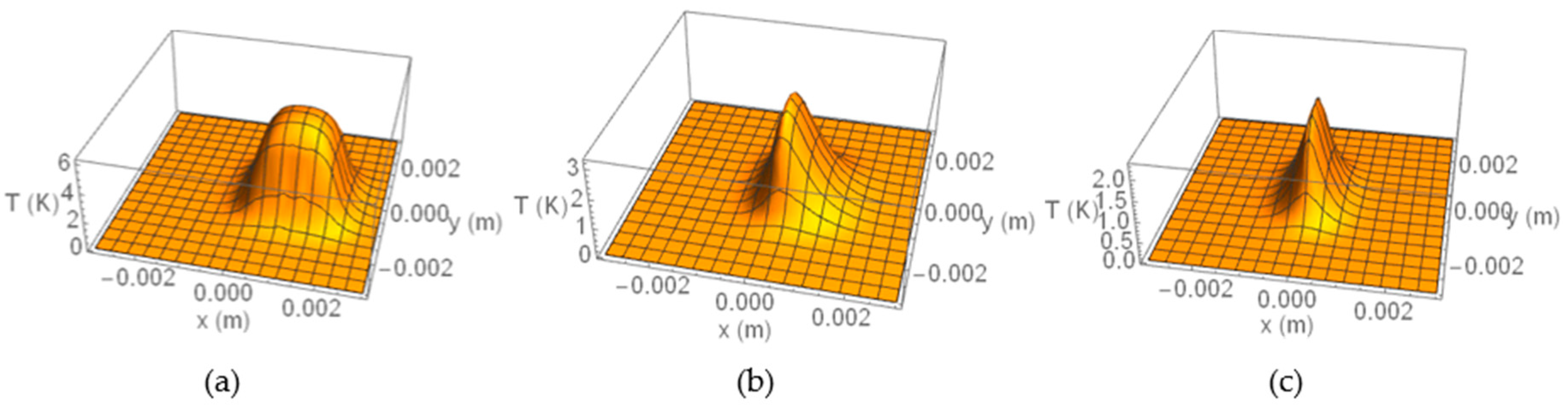In Figure 2, we present surface temperature distributions calculated at the end of a τ = 1 s burst, T(x,y,0,τ), using Equation (10) with K = 0.5 W/mK and D = 1.3 ∙ 10⁻⁷ m²/s (thermal properties of the photo-polymeric resin used in the experiments) produced by a square heat source (w = h = 2 mm) emitting a power density of Φ = 10 kW/m² (total emitted power 40 mW), whose upper side is buried d = 0.1 mm below the surface. From now on, all the calculations will be performed for these material properties. We show three inclinations of the heat source: (a) parallel to the surface, φ = 0°, (b) at an angle of φ = 30° with respect to the surface, and (c) a vertical heat source, perpendicular to the surface (φ = 90°). As can be seen, the angle of inclination has a noticeable impact on the surface temperature, both on the temperature elevation and on the particular distribution. The temperature elevation caused by the horizontal heat source is the highest one because for φ = 0° the whole area producing heat is buried d = 0.1 mm, whereas for increasing φ (notably for the vertical heat source, φ = 90°), the positions emitting heat are buried deeper below the surface.

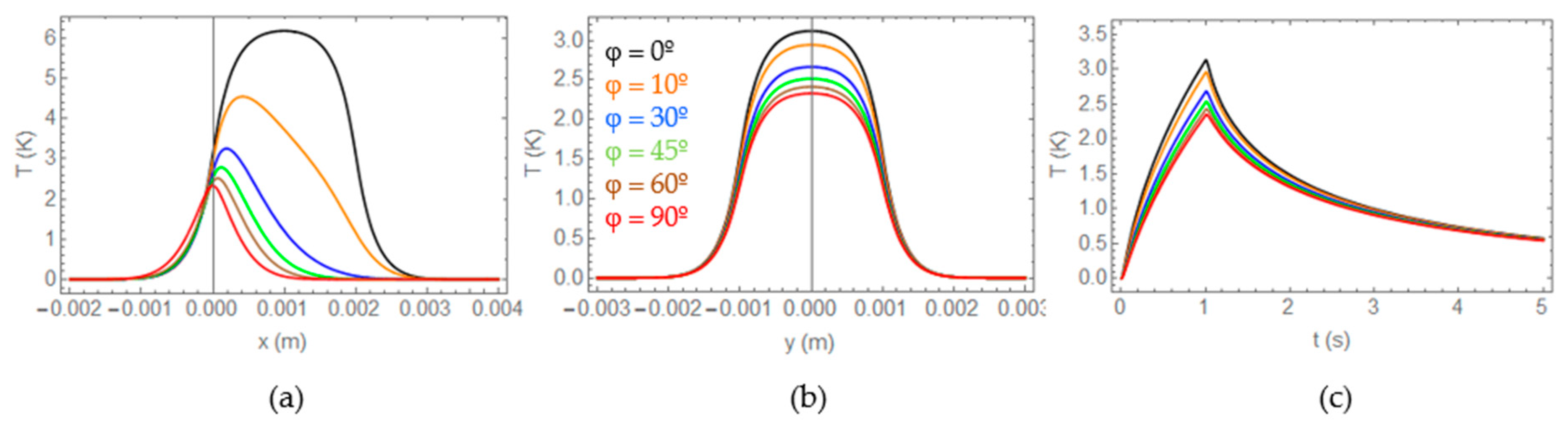
As the inclination of the heat source has the direction of the OX-axis, the surface temperature distribution is mostly affected in this direction. To illustrate this, in Figure 3a,b we present surface temperature profiles along the OX- and OY-directions, T(x,0,0,τ) and T(0,y,0,τ), respectively, produced by heat sources of the same dimensions, depth, flux, and burst as in Figure 2, for six different inclinations φ = 0°, 10°, 30°, 45°, 60°, 90°. As pointed out in Figure 2, the OX-profiles are asymmetric, except for the horizontal (φ = 0) and vertical (φ = 90°) heat sources although, according to the geometry depicted in Figure 1, the former is displaced with respect to the origin. The inclination does not significantly affect the shape of the OY-profiles, which remain symmetric.

Figure 3c shows the evolution of the temperature at the origin T(0,0,0,t) for the same heat sources. Similarly to the OY profile, the inclination does not significantly affect the shape of the temperature-time curve.

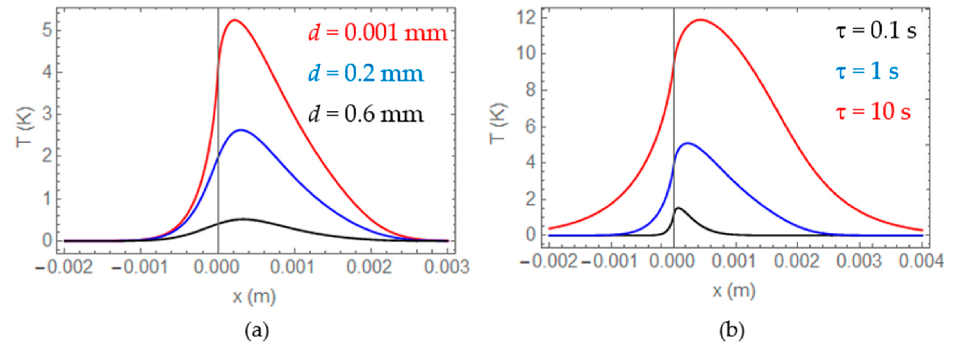
According to the previous results, we can infer that the inclination of the heat source affects mainly the shape of the temperature distribution along the OX direction, featuring an asymmetry. However, the evidence of this signature depends on the depth d of the heat source and the duration of the burst, τ. As an example, Figure 4a displays OX profiles calculated at the end of a τ = 1 s burst, T(x,0,0,τ), produced by a squared heat source of the same dimensions (w = h = 2 mm) and flux (Φ = 10 kW/m²) as in Figure 3, that makes an angle of φ = 20° with the surface, for three different depths, d = 0.001, 0.2, and 0.6 mm. We can see that, as the depth increases, not only the signal diminishes, but also the curve is smoothed out, making the identification of the angle more difficult. In Figure 4b we illustrate the dependence of OX-profiles with the duration of the burst. We show T(x,0,0, τ) corresponding to a heat source buried d = 0.01 mm, with the same geometry and heat flux as in Figure 4a, calculated at the end of three different bursts, τ = 0.1, 1, and 10 s. For this geometry, the deepest side of the rectangle is buried d_max = 0.69 mm below the surface.

As can be seen, the duration of the burst has a significant impact on the OX temperature profiles calculated at the end of the burst. If the burst is short (τ = 0.1 s, associated thermal diffusion length ${\mu }_{\tau }=\sqrt{4D\tau }$= 0.23 mm, black line), the asymmetry of the profile is very pronounced because the heat produced at the deepest side of the square does not have time to reach the sample surface by the end of the burst. As the burst increases (τ = 1 s, μ_τ = 0.72 mm, blue line), the information coming from deeper locations has reached the surface by the end of the burst, still featuring a noticeable asymmetry, characteristic of the inclination. If the burst is long (τ = 10 s, μ_τ = 2.3 mm, red line) the heat coming from any position of the heat source has reached the surface. The profile contains information from all locations and is smoothed out by diffusion. It can also be noticed that in this evolution with τ, the position where the temperature is maximum at the end of the burst moves to the right, i.e., towards the geometrical center of the heat source.

The previous analysis points out that the duration of the burst might affect the accuracy with which the dimensions, depth, and orientation of a rectangular heat source is determined. In the next section, we present a sensitivity analysis aimed at studying the optimum conditions to characterize rectangular heat sources of any inclination.

3. Sensitivity

In order to compare sensitivities to different parameters, we define the sensitivity of the surface temperature to a given parameter p as:

$$\mathit{S}\mathit{p}=\mathit{p}\frac{\mathit{\partial }\mathit{T}}{\mathit{\partial }\mathit{p}},\hspace{1em}\hspace{1em}\mathit{p}=\mathit{w},\hspace{0.17em}\mathit{h},\hspace{0.17em}\mathit{d},\hspace{0.17em}\mathit{\phi }$$

(12)

In the following, we analyze the sensitivity of the surface temperature to the parameters characterizing the geometry and location of the heat source, namely, the width w, the height h, the depth d, and the angle φ. For the sensitivity analysis, we consider a standard squared heat source of dimensions w = h = 1 mm. In order to highlight the influence of the burst duration τ, we consider a challenging case: a vertical heat source (φ = 90°), buried below the surface d = 0.5 mm, and excited with a short τ = 0.5 s burst (μ_τ = 0.51 mm). Figure 5a–d displays the sensitivities Sw, Sh, Sd, and Sφ, calculated at t = τ = 0.5 s, for Φ = 40 kW/m² (total emitted power 40 mW as in Figure 2, Figure 3 and Figure 4).

As can be seen, the highest sensitivity corresponds to the width, as the width information is available at the shallowest positions of the crack. The maximum values of this sensitivity appear at the location of the lateral ends of the square. The second most sensitive parameter is the angle which, for φ = 90°, exhibits a bi-modal shape in the direction of the inclination (OX-axis): as the angle increases, the temperature increases for $x\le 0$ and decreases at positive values of the x coordinate. The next parameter in decreasing sensitivity order is the depth, which is negative as the temperature at the surface decreases for increasing depth. The height of the heat source is the less sensitive parameter, as it corresponds to changes at positions located at the maximum depth. For the particular situation analyzed, the deepest end of the heat source is buried d_max = 1.5 mm below the surface, whereas the thermal diffusion length associated to the end of the burst is μ_τ = 0.51 mm, as mentioned above. This is the reason why the values of Sh are so low. Very interestingly, the positions where the maximum sensitivities occur for the different parameters are well separated spatially, except for the height and the depth, for which the maximum sensitivity is located around the origin, in this configuration. Accordingly, we can conclude that the width w and angle φ are decorrelated with each other and also with height h and depth d, but these two might be correlated, as far as the surface temperature at the end of the burst is concerned. However, if we look at the sensitivities of the temperature evolution at the origin T(0,0,0,t) to the height and the depth (Figure 5e), we notice that the maximum sensitivities to h and d occur at different instants and thus these parameters are not correlated in the timing-graph at the origin. It is also remarkable that, because the burst is short (μ_τ < d_max), as already mentioned, the sensitivity of the spatial information to h is very low (Figure 5b), whereas the timing-graph at the origin features a much higher sensitivity, which appears after the end of the burst. It is worth noting that the previously mentioned correlation between Sh and Sd, only occurs for this challenging case of a vertical crack. In Figure 5f, we show OX profiles of Sd and Sh calculated for the same w = h = 1 mm crack buried d = 0.5 mm below the surface and excited with the same burst, τ = 0.5 s, but making an angle of φ = 30° with the surface. The displacement of the maxima of the curves clearly demonstrates the lack of degeneracy between the two magnitudes. Moreover, a comparison between the sensitivity values of Sd and Sh in Figure 5f, for φ = 30°, and in Figure 5b,c for φ = 90°, illustrates the fact that the sensitivities to the lateral dimensions and depth of the heat source increase when the inclination decreases. Finally, it is worth noting that, regarding the thermogram at the end of the burst, T(x,y,0,τ), OX- and OY- axes summarize all relevant sensitivity information on the four parameters: OX-axis on Sw, OY-axis on Sφ, and both OX- and OY-axes, on Sh and Sd.

According to this sensitivity analysis, we can conclude that gathering the temperature profiles obtained at the end of the burst along OX- and OY-axes (T(x,0,0, τ) and T(0,y,0, τ)) and the timing-graph at the origin (T(0,0,0,t)), we combine spatial and temporal information for which the sought parameters w, d, h, and φ are not correlated and thus we should be able to retrieve the geometrical characteristics of the crack univocally. Furthermore, this reduction of data enables a computationally efficient fitting and thus, a fast characterization of the heat source.

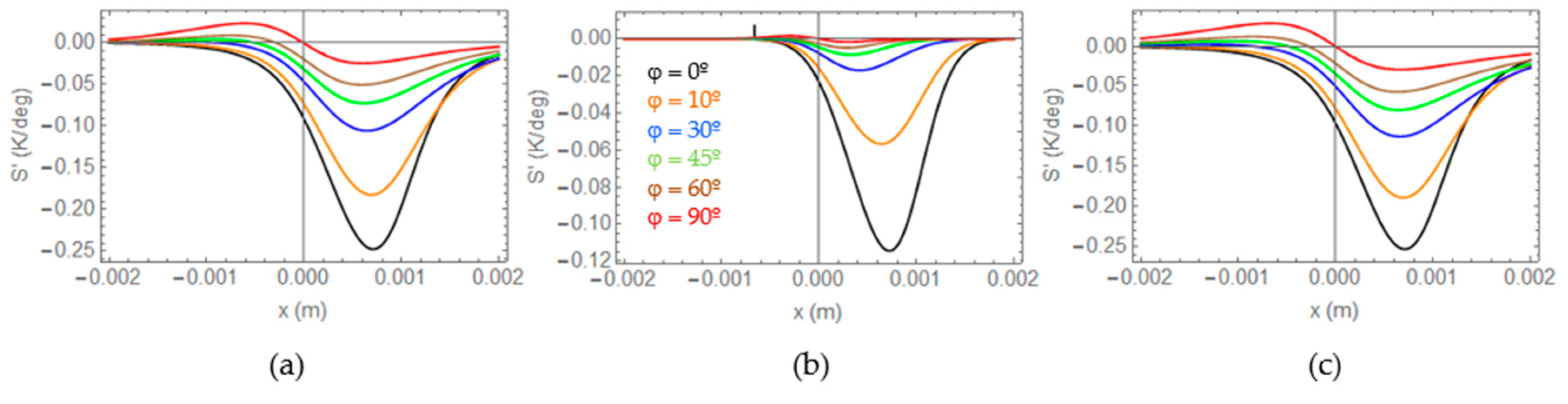
We focus now on the sensitivity to the angle. The definition of sensitivity given by Equation (12) was useful to compare sensitivities to different parameters (Figure 5). However, in order to compare the sensitivity of the surface temperature to the angle for different orientations of the heat source, the definition is not appropriate because the product of the derivative by the actual angle penalizes low angles. In the limit, for a horizontal heat source, the definition gives zero sensitivity, which is nonsense. Accordingly, in order to compare the sensitivities to the angle for different angles, we introduce a new definition:

$$S^{\prime }=\frac{\partial T}{\partial \phi }$$

(13)

In Figure 6a, we represent S’ along the OX-axis at the end of a τ = 5 s burst (μ_τ = 1.6 mm) for the same standard heat source (w = h = 1 mm) buried d = 0.5 mm below the surface emitting a flux of Φ = 40 kW/m², and several inclinations, namely, φ = 0°, 10°, 30°, 45°, 60°, and 90°. For φ = 90°, the maximum depth of the heat source is d_max = 1.5 mm, of the same order as μ_τ.

The sensitivity is maximum for the horizontal heat source, φ = 0° and minimum for the vertical source, φ = 90°, with a relationship of 10/1. However, if the duration of the burst corresponds to a thermal diffusion length μ_τ significantly shorter than d_max, then the maximum to minimum sensitivity relationship is much larger. As an example, in Figure 6b we show the sensitivities for τ = 0.5 s corresponding to a thermal diffusion length of μ_τ = 0.51 mm, just coinciding with the depth of the upper side of the square. In this case, the maximum to minimum sensitivity relationship is of the order of 100/1. This points at the benefit of using long enough bursts, guaranteeing that the entire heat source is located within one thermal diffusion length from the surface. However, once this condition is fulfilled, further increasing the duration of the burst does not provide more sensitivity to the angle. This can be confirmed in Figure 6c, where we show the same sensitivity profiles as in 6a and 6b, but for a burst of τ = 10 s, corresponding to a thermal diffusion length μ_τ = 2.3 mm. A comparison between Figure 6a,c confirms that once μ_τ > d_max, an increase in thermal diffusion length does not improve the sensitivity to the angle.

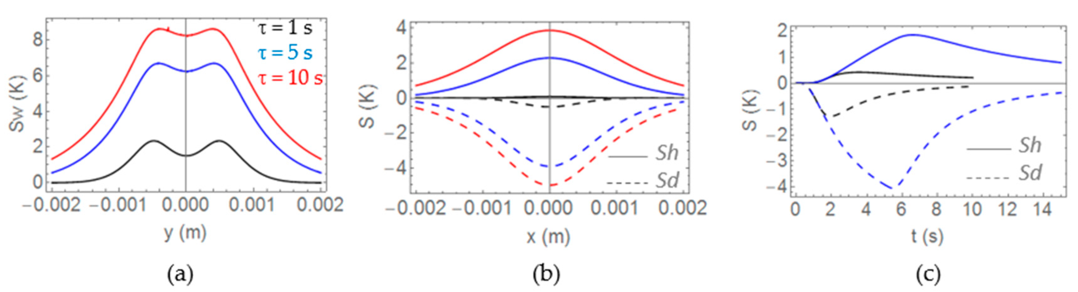
Increasing the duration of the excitation τ increases the sensitivity to the rest of the parameters, as well. In Figure 7a,b we display sensitivities (original definition in Equation (12)) of the temperature distribution at the end of the burst along the coordinate-axes to the magnitudes featuring the most significant variation along each axis (see Figure 5a–d): OY profile for Sw (Figure 7a) and OX profiles for Sh, Sd (Figure 7b). In all cases, w = h = 1 mm, d = 0.3 mm and φ = 90° (d_max = 1.3 mm), and we represent three bursts, namely, τ = 1 s (μ_τ = 0.72 mm, black), τ = 5 s (μ_τ = 1.6 mm, blue) and τ = 10 s (μ_τ = 2.3 mm, red). Figure 7c displays Sh and Sd of the timing graph at the origin, T(0,0,0,t) for τ = 1 and 5 s.

As in the case of the angle, the values of sensitivities tend to saturate for bursts with associated thermal diffusion lengths fulfilling μ_τ > d_max. In the case of Sw (Figure 7a), an increase in the duration of the burst also entails a loss of contrast in the valley located at the center of the curve. This loss of contrast can eventually evolve towards the disappearance of the valley, leading to a certain degree of degeneracy of Sw with Sd and Sh. Figure 7b shows that Sd and Sh of T(x,0,0,τ) for τ = 5 s increase dramatically with respect to τ = 1 s as the thermal diffusion length associated to the end of the burst increases from μ_τ = 0.72 mm for τ = 1 s, to μ_τ = 1.6 mm for τ = 5 s: the former covers about half of the area of the heat source whereas later includes the whole emitting area. The comparison of the maximum Sh and Sd of T(x,0,0,t) and T(0,0,0,t) (Figure 7b,c, respectively) for τ = 1 s, reveals that for short bursts the sensitivities to the depth and the height are higher for the timing graph at the origin, T(0,0,0,t), as pointed out in Figure 5. This confirms the proposed data selection (T(x,0,0,τ), T(0,y,0,τ), and T(0,0,0,t)), combining spatial and temporal information, as adequate data for the fast characterization of these heat sources. Moreover, for τ = 5 s the sensitivities Sd and Sh of T(x,0,0,τ) (Figure 7b) are similar to the sensitivities of T(0,0,0,t), (Figure 7c), which still break the degeneracy of Sd and Sh in T(x,y,0,τ).

As a summary, increasing the duration of the burst increases the sensitivity asymptotically, but at the expense of an eventual degeneracy of Sw with Sd and Sh, that does not occur for short bursts. A rule of thumb could be to use the shortest excitation that covers the depth that needs to be proved. It is worth noting that the analysis presented in this section can be extrapolated to other material properties, heat source dimensions, and depths, and excitation durations, provided that the thermal diffusion length associated to the end of the burst, μ_τ, keeps the same relationship with w, h, and d.

4. Fittings of Synthetic Data

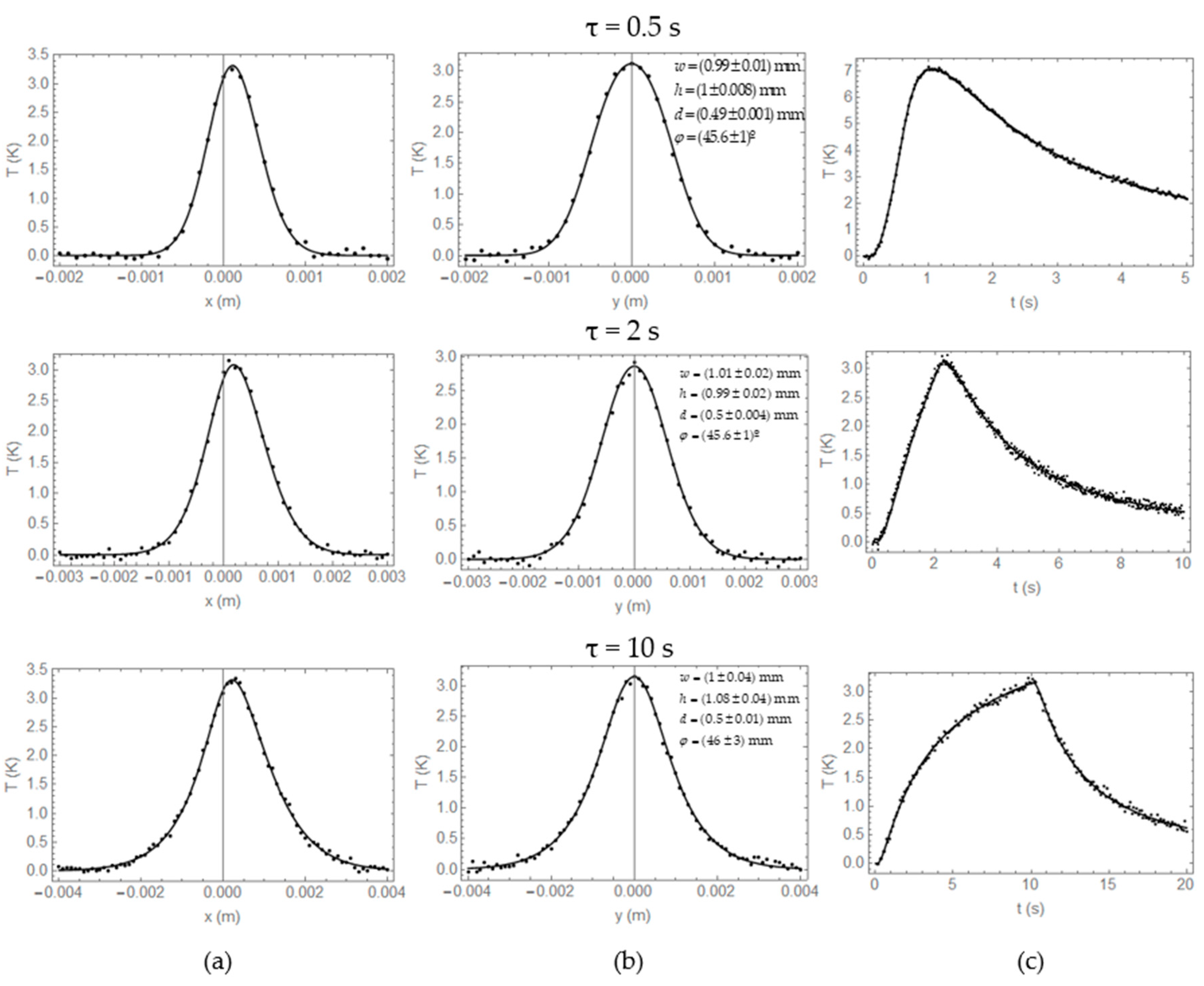
In this section we present fittings of Equations (10) and (11) to synthetic T(x,0,0,τ), T(0,y,0,τ) and T(0,0,0,t) data calculated for rectangular heat sources of different orientations in a thermal isolator (D = 0.13 mm²/s, K = 0.5 W/mK) with added Gaussian noise with zero mean and normal distribution. The fitting parameters are Φ, w, h, d, and φ. We analyze the effect of the signal to noise ratio in the data and of the duration of the burst on the accuracy of the retrieved values of the five fitting parameters.

We start considering a standard w = h = 1 mm square heat source, buried d = 0.5 mm below the surface at an intermediate inclination of φ = 45°. The maximum depth of this heat source is d_max = 1.2 mm. In Figure 8 we present synthetic data calculated for three bursts τ = 0.5, 2, and 10 s, corresponding to thermal diffusion lengths of μ_τ = 0.51, 1, and 2.3 mm respectively. In order to separate the effect of the noise in the data from the mere effect of the duration of the burst τ, all data sets feature the same signal to noise ratio, SNR = 60 at T(0,0,0,τ), i.e., T(0,0,0,τ) = 3 K and noise of 50 mK.

As can be seen, for a SNR of 60 the fittings provide sensible values of the geometrical parameters defining the crack in the whole burst range, which confirms the adequacy of the selected information to characterize the heat source. However, the quality of the results does depend on the SNR.

As an illustration, in Figure 9 we present best fit parameters and standard deviations corresponding to the same heat source as in Figure 8 (w = h = 1 mm, d = 0.5 mm, φ = 45°), excited with a τ = 5 s burst, obtained from data featuring different values of the SNR. For this τ, the thermal diffusion length associated to the end of the burst, μ_τ = 1.6 mm, largely covers the maximum depth of the heat source d_max = 1.2 mm.

In all cases, both the accuracy but especially the precision of the estimated parameters decrease with decreasing SNR. However, the plots show different responses of the fitting parameters to noise. If we focus on the estimated w, h, and d (note that the vertical scales on Figure 9a–c span the same parameter range), the height h is the parameter most affected by noise, with an uncertainty that varies from 20% to 1% for SNRs ranging between 15 and 150. The depth and the width exhibit similar relative uncertainties, although the accuracy is higher for the depth estimation in all SNRs. This might be due to the effect of the relatively long burst, that washes out the signature of the width. Finally, regarding the estimation of the angle (Figure 9d), the accuracy is very stable but the increase in uncertainty with decreasing SNR is the most pronounced. As a summary, the results show that even for SNR as low as 15, the accuracy of the retrieved parameters is better than 10%. These general trends are similar for other depths, with reduced uncertainty and increased accuracy for shallower heat sources.

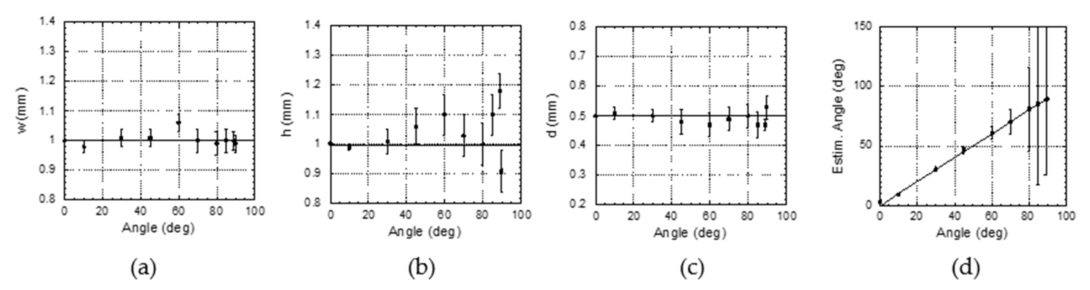
Let us analyze now the effect of the angle of the heat source on the quality of the retrieved parameters. In Figure 10, we present values of the retrieved w, h, d, and φ for the same standard heat source w = h = 1 mm, buried d = 0.5 mm below the surface, as a function of the inclination φ, also excited with a τ = 5 s burst. The signal to noise ratio of the data is SNR = 60.

Inspection of Figure 10a–d reveals a slight decrease of the quality of the retrieved width w, and depth d with increasing angle, in terms of both accuracy and precision. However, the estimation of the height of the heat source is strongly affected by the inclination, as the parameter of interest, i.e., the deepest side of the heat source is buried deeper with increasing angle. This loss of quality affects both accuracy and precision. As for the estimation of the angle, the accuracy stays very good, but the uncertainty increases dramatically for heat sources approaching the vertical. It is worth mentioning that in all cases analyzed, the accuracy and precision in the estimation of the emitted power is better than 5%. These results are in agreement with the sensitivity analysis summarized in Figure 6.

As a summary, we can conclude that it is possible to determine the lateral dimensions, the depth and the inclination of buried rectangular heat sources. The duration of the burst does not significantly affect the quality of the retrieved parameters, whereas the SNR might eventually jeopardize precision of the retrieved values, mostly the height and the inclination of the heat source. For SNR above 50 and angles below 45°, the uncertainty stays below 5%.

5. Experiments and Results

In this section we present fittings of experimental data obtained with an inductive thermography set-up on samples containing calibrated metallic inclusions. We have prepared 3D printed photopolymer resin (PR48) samples, whose thermal conductivity and diffusivity are K = 0.5 W/mK and D = 1.3 · 10⁻⁷ m²/s respectively, with embedded thin Cu slabs. The dimensions of the resin samples are 2.5 × 2.5 × 1 cm. During 3D printing, the process is stopped, a Cu slab is placed on the hot resin, and printing is resumed. The Cu films are 25 μm thick. We have prepared three samples containing Cu films of different lateral dimensions, depths, and inclinations with the surface. The specific values of w, h, d, and φ are listed in

Table 1. Real and retrieved sizes of the Cu films of the three samples used in the experiments.

Sample		w (mm)	h (mm)	d (mm)	φ (deg)	Flux (kW/m2)
Sample 1 (Current: 15 A)	Fitted values Real values	2.3 2.1	1.2 2.1	0.38 0.4	69 60	66.5 -
Sample 2 (Current: 10 A)	Fitted values Real values	2.5 2.2	1.4 1.8	0.26 0.28	38 30	61 -
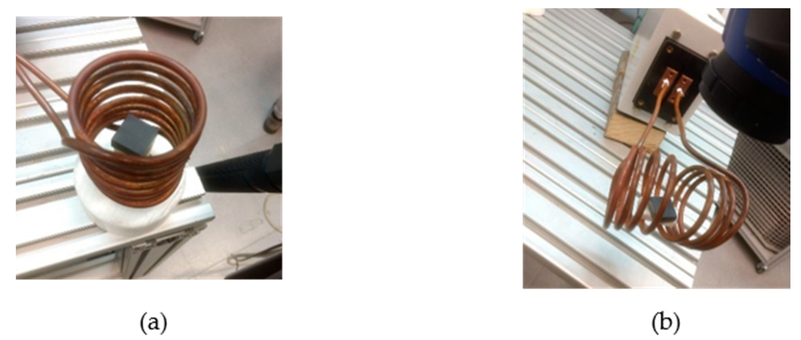
Sample 3 (Current: 10 A)	Fitted values Real values	2.8 2.5	2.6 2.2	0.24 0.27	9.7 0	80 -

. We put the sample inside an 8 cm diameter coil, with the Cu slab oriented mostly perpendicular to the coil axis. This way, when the coil is fed with an AC current, Eddy currents flow in closed paths within the Cu slab plane, which is heated by the Joule effect, producing a geometrically calibrated heat source. The high conductivity of Cu ensures a fast thermalization of the film, even if the current density is not perfectly homogeneous. The excitation power and frequency are 11 kW and 120 kHz, respectively. The IR radiation coming from the sample surface is collected by an IR video camera equipped with a 320 × 256 pixel detector, sensitive in the 3.5–5 μm range, and with a noise equivalent temperature difference (NETD) of 25 mK. The camera is operated at 100 frames per second and integration time of 4 ms. It was shielded to prevent damage from the AC current in the coil. Although the resin is opaque in the detection range of the camera, the surface where the temperature is measured is covered with a thin layer of graphite paint to improve IR emissivity. Figure 11 shows pictures of the coil with the sample in place for Cu slabs making angles with the surface φ < 45° (Figure 11a) and φ > 45° (Figure 11b).

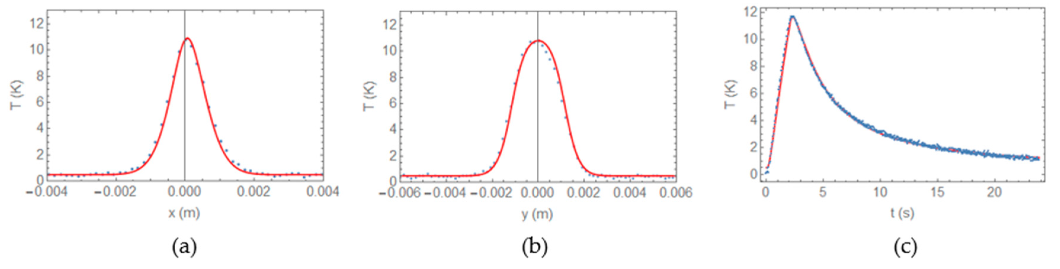
In Figure 12, we show in symbols experimental T(x,0,0,τ), T(0,y,0,τ) and T(0,0,0,t) obtained at the end of a τ = 2 s burst, corresponding to sample 1, where a Cu slab of dimensions w = h = 2.1 mm, making an angle of φ = 60° with the surface is buried at d = 0.4 mm. The spatial resolution is 0.175 mm/pixel. The solid lines are the best fittings of Equation (10) (Figure 12a,b) and Equations (10) and (11) (Figure 12c) to the data.

The values of the best fit parameters are w_f = 2.3 mm, h_f = 1.2 mm, d_f = 0.38 mm and φ = 75°. As expected, the parameter with the worst estimation is the height of the heat source, but the rest of the retrieved parameters are in good agreement with the true values: the retrieved width is off by 10%, the angle by 9°, and the depth only by 0.5%.

In Table 1 we summarize the real and fitted parameters corresponding to the three samples we prepared, with Cu slabs making angles of 0°, 30°, and 60° with the surface. In all cases the duration of the excitation was τ = 2 s. We do not have an independent calibration of the emitted flux, but we record the values of the current feeding the coil in each experiment.

The results point at the difficulty of identifying the height of the heat source, especially for heat sources close to the vertical. However, the width and depth can be assessed with an accuracy of about 10%, in experimental data. The inclination of the heat source has been retrieved in good qualitative agreement with the true angles, with uncertainties of about 9°. It is worth noting that the retrieved fluxes seem sensible given the current values and orientation of the Cu slabs with respect to the coil axis. Samples 2 and 3 were excited with the same coil current but the retrieved flux is less for sample 2, as the Cu slab makes an angle with the coil axis. In sample 1, excited with a higher current, the retrieved flux is also higher. Even with the difficulty associated to the estimation of h, the fittings of experimental results confirm that it is possible to evaluate the lateral dimensions, inclination and emitted flux of inclined planar heat sources. To the best of our knowledge, these are the first quantitative results reported on the geometrical parameters and flux of buried tilted heat sources from surface temperature data.

6. Summary, Conclusions, and Outlook

The possibility of identifying the dimension, depth and orientation of planar heat sources buried below the surface from IR thermography surface temperature data in time domain has been analyzed. These heat sources are representative for defects that produce heat under any type of excitation, such as cracks excited with ultrasounds or metallic inclusions in electrical insulators excited inductively. A sensitivity analysis has been conducted showing that two perpendicular surface temperature profiles measured at the end of the burst together with the temperature history at one position of the surface gather the spatial and temporal information needed to retrieve the lateral dimensions, inclination, depth, and flux of tilted squared heat sources, univocally. The sensitivity study also shows that optimum results are obtained when the thermal diffusion length associated to the duration of the burst coincides with the maximum depth at which heat is emitted: for shorter bursts the sensitivity to the height might be too low and longer bursts harm the decorrelation between parameters. A sensible rule of thumb could be to use the shortest burst able to sense the target layer under inspection. The fittings of synthetic data with added noise show that the quality of the results worsens as the SNR is reduced and the inclination of the heat source approaches the vertical. Fittings of experimental data confirm that the height of the heat source is the most challenging parameter, especially when the heat source makes an angle higher than 45° with the surface. The width and depth can be retrieved within 5 to 10% and the angle within 9° from the true value.

This first study proves that it is possible to characterize rectangular tilted heat sources from surface temperature data obtained by infrared thermography. However, there is still room to improve the experimental results in several aspects. The first question refers to the protection of the infrared camera against the effect of the electromagnetic field. This effect may eventually harm the electronic system of the camera but also induces noise in the data during the excitation period. In addition to the protection of the camera itself and the associated noise reduction, an improved shielding would also allow to reduce the distance between the camera and the sample/coil system, thus improving the spatial resolution in the experiments, which is highly desirable for heat sources with dimensions similar to the ones handled in this work. Another aspect to pay attention to is the quality of the samples, in terms of eventual lack of adherence between the Cu slab and the resin, which can lead, among others, to unwanted thermal resistances and distorted temperature distributions.

Finally, regarding future perspectives and with the aim of characterizing tilted planar defects that produce heat in thermographic nondestructive testing techniques, the next step is the characterization of planar, tilted heat sources of arbitrary shape. The conclusions drawn from this study suggest that some additional information both spatial and temporal, might be necessary to characterize defects of any shape. Nevertheless, these first quantitative results open the possibility of characterizing tilted flaws in any thermographic modality with internal thermal excitation of defects.