Article

Investigation of the Influence of Excess Pumping on Groundwater Salinity in the Gaza Coastal Aquifer (Palestine) Using Three Predicted Future Scenarios

1
Department of Civil Engineering and Geomatics, Durban University of Technology, 4001 Durban, South Africa
2
Department of Engineering Sciences, University College of Science and Technology, Khan Yunis, Palestine
3
Institute for Water and Wastewater Technology, Durban University of Technology, 4001 Durban, South Africa
4
Department of Environmental Engineering, The Islamic University of Gaza, Gaza, Palestine
5
Civil Engineering Programme, University College of Technology, Sarawak 96000, Malaysia
6
Civil Engineering Department, University of Malaya, Kuala Lumpur 50603, Malaysia
7
Civil Engineering Department, Dokuz Eylul University, 35210 İzmir, Turkey
*
Author to whom correspondence should be addressed.
Water 2020, 12(8), 2218; https://doi.org/10.3390/w12082218
Submission received: 20 April 2020 / Revised: 8 July 2020 / Accepted: 21 July 2020 / Published: 6 August 2020
(This article belongs to the Special Issue Groundwater Resilience to Climate Change and High Pressure)

Abstract

:
The Gaza coastal aquifer (GCA) is the only source of water for about two million citizens living in Gaza Strip, Palestine. The groundwater quality in GCA has deteriorated rapidly due to many factors. The most crucial factor is the excess pumping due to the high population density. The objective of this article was to evaluate the influence of excess pumping on GCA’s salinity using 10-year predicted future scenarios based on artificial neural networks (ANNs). The ANN-based model was generated to predict the GCA’s salinity for three future scenarios that were designed based on different pumping rates. The results showed that when the pumping rate remains at the present conditions, salinity will increase rapidly in most GCA areas, and the availability of fresh water will decrease in disquieting rates by 2030. Only about 8% of the overall GCA’s area is expected to stay within 500 mg/L of the chloride concentration. Results also indicate that salinity would be improved slightly if the pumping rate is kept at 50% of the current pumping rates while the improvement rate is much faster if the pumping is stopped completely, which is an unfeasible scenario. The results are considered as an urgent call for developing an integrated water management strategy aiming at improving GCA quality by providing other drinking water resources to secure the increasing water demand.

1. Introduction

The main source of drinking water in the Gaza Strip is a shallow aquifer, which is part of the coastal aquifer. The quality of the groundwater has extremely deteriorated in terms of salinity and nitrate concentrations. Salinity in the Gaza coastal aquifer (GCA) is characterized by a high chloride concentration, depending on the location and other hydrochemical processes [1,2]. Various processes may cause salinization of the groundwater, including seawater intrusion, movement of saltwater from the deeper layers of the aquifer, contribution from discharges from older formations surrounding the coastal aquifer, and dissolution of soluble salts in the aquifer. The root cause of the aforementioned GCA salinization processes is the unbalance of the groundwater system resulting from overpumping in the Gaza area, which is considered among the most populated regions in the world [3,4]. In addition, potential man-induced (anthropogenic) sources, including agricultural return flows, wastewater seepage, and leachate from solid waste dumping sites, are involved in increasing groundwater salinity [5,6,7].
Modeling groundwater quality using traditional numerical modeling techniques consumes a lot of effort and requires a large amount of data. Therefore, artificial intelligence techniques have become very popular and efficient tools for modeling complicated processes using relatively less cost and effort. It thus provides an easy and efficient tool for groundwater quality modeling [2,8,9,10].
The decision to choose any of the modeling techniques mainly depends on two elements: First, the available amount of understanding of the physical behavior of the process, and second, the availability of hydrogeological data that describe the related variables. In the case of sufficient understanding of both the physical process and the data, process-based models are the suitable modeling technique. The model in this case is developed depending on the physical understanding of the process. The model may then be calibrated using the available data. In the case of sufficient data but insufficient understanding of the physical process, AI-based models are the suitable modeling technique. If both the data and understanding of the physical process are insufficient, statistical methods can be applied only as an initial tool to improve the general understanding of the groundwater salinization process [11,12]. After the data collection process in the study area, it was noticed that the description of the physical characteristics of the groundwater and the related parameters have not been sufficiently addressed and described yet. However, enough data have been successfully collected. Accordingly, AI-based models are the most suitable modeling technique for groundwater prediction and modeling based on the availability of sufficient modeling data.
As a result of the complex nonlinear relationship, there is no direct scientific formula that correlates the effect of pumping on groundwater salinity. Therefore, the artificial intelligence approach is considered a suitable option to model such a relationship [3,13]. The strength of AI techniques originated from their ability to simulate the human brain’s behavior to solve complex problems [14]. As one of the AI techniques, artificial neural network (ANN) structures are composed of input, output, and at least one hidden layer, each of which has one or more simple interconnected adaptive elements called ‘nodes’ that have a high ability to perform a huge number of parallel computations.
Although the safe yield of GCA is only 50 to Mm3/year, the total consumption from the groundwater resources in the Gaza Strip in is about 170 Mm3/year. In groundwater management, the concept of safe yield has been used to state the limits of pumping rates from a groundwater basin. It is the attainment and maintenance of a long-term balance between the amount of groundwater withdrawn annually and the annual amount of recharge. Thus, it limits the pumping rate to the amount, which is replenished naturally through precipitation and surface-water seepage. The soil recharge coefficients for GCA have been estimated in the Coastal Aquifer Management Program (CAMP). The recharge rate is then calculated based on the long-term annual precipitation [15,16]. This implies overpumping of about three times of the safe yield, and consequently leads to the deterioration of the groundwater quality [17,18]. Since the safe yield is expressed as a single annual average rate, associated limitations on diversions in water allocation permits and on contractual obligations of water allocation permittees should also be on an annual average basis. Because of the uncertainties inherent in safe yield estimates, they should be rounded in accordance with standard mathematical practice to no more than three significant figures. Each specific alternative, configuration, or scenario of a safe yield simulation model should be run iteratively, for the period of record, with various trial annual average system drafts to determine the annual average system draft that would divert all usable storage volumes of water from the system’s reservoir(s). For each specific alternative, configuration, or scenario of a safe yield simulation model, simulated usable storage volumes of water normally vary over the period of the record and the restrictive condition that limits the safe yield estimate is the diversion of all usable storage volumes of water as described in the paragraph above during any one day of the period of the record. The drought during which this restrictive condition occurs is the most severe drought of the record [19,20].
The main source of the elevated concentration levels of chloride concentration Cl in GCA is the overpumping. During the last decades, GCA has been extensively overexploited due to the increasing population growth, high rates of urbanization, and increased agricultural activity. Intensive exploitation of groundwater in the Gaza Strip in the past years has disturbed the natural equilibrium between fresh and saline water, and has resulted in increasing salinity. This has induced seawater to flow towards the major pumping centers in urban areas leading, to continuous increasing of the levels of Cl in GCA, particularly in areas close to the coastline [7,21]. It has been found that seawater intrusion extends about 2 km inland in many areas of Gaza Strip [7]. Lateral flow from the eastern Eocene aquifer is another source of CL. Such an aquifer is characterized by high Cl levels, and its flow regime is normally to the west towards GCA. Consequently, water flux coming from the Eocene aquifer worsens ground water quality by increasing Cl levels, especially in the eastern parts of Gaza Strip [22,23]. Saline lenses, which are found in many GCA locations particularly in the southern parts, are salty water lenses existing at deeper layers. Hence, if the wells are near these lenses and the screens are deep enough, these lenses participate in feeding these wells and the abstracted water from these wells will have elevated Cl concentrations [22,23,24]. Many other Cl sources, such as the recharge of irrigation water and percolation of landfill leachate, contribute to the deterioration of the ground water quality [22,23].
The objective of this study was to evaluate the response of GCA to the excess pumping from groundwater and analyze the future deterioration of groundwater salinity using three future scenarios to predict groundwater salinity in 2030 by developing and generating an empirical model developed using ANNs. Understanding the relationship between groundwater pumping and the deterioration of salinity can contribute to integrated water resources management in the Gaza area.

2. Study Area and Modeling Tool

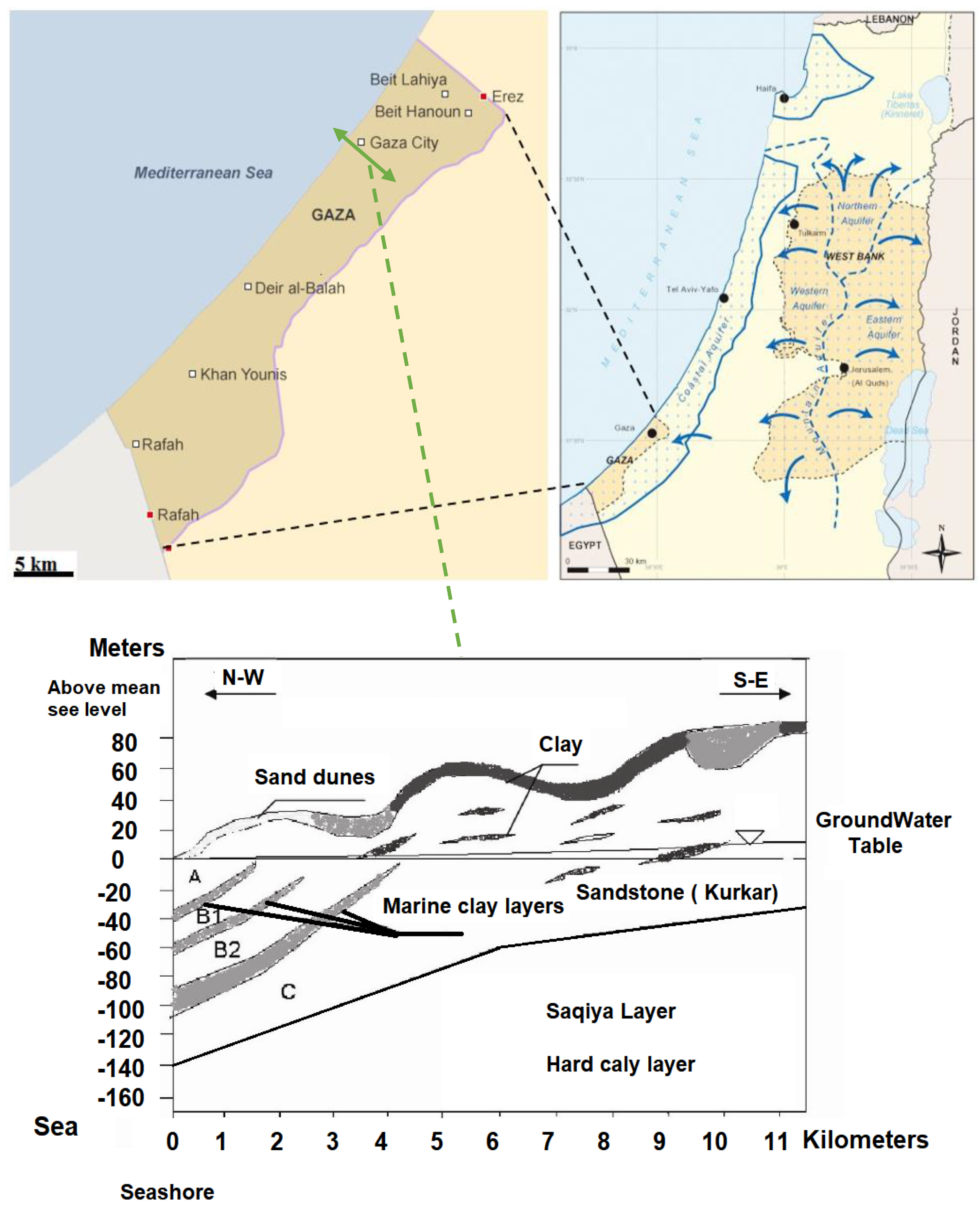
2.1. Geology and Hydrogeology of the GCA

The study area of this research was the Gaza Strip, Palestine. It is a narrow strip of land on the Mediterranean coast. It is part of Palestine with an area of about 365 km2 and it is around 40 km long [25]. Figure 1 shows the regional and location map of the Gaza Strip. The Gaza Strip is an area where the exploitation level of recourses exceeds the carrying capacity of the environment. This is especially true for the water and land resources, which are under high pressure and subject to overexploitation, pollution, and degradation. The salinity of the groundwater is a main difficult issue in the Gaza Strip. GCA is part of the coastal aquifer that extends from GS in the south to Carmel Mountains in the north along the Mediterranean coast line (about 120 km), as shown in Figure 1, which illustrates the layout of GCA and the adjacent aquifers [25]. The width of GCA varies from10 km in the north to about 20 km in the south [22,26]. The GCA thickness varies from about 120 m in the west (at the shoreline) to a few meters in the east [27]. Meanwhile, the depth of the water level of GCA ranges from about 60 m below the ground surface in the east to a few meters near the coastline in the west [25].
Within Gaza Strip, the coastal aquifer overlies the saqiye group, which is considered to be impermeable. The top of the saqiye group therefore marks the base of the coastal aquifer. Approximately 10 to 15 km inland from the coast, the saqiye group pinches out, and the coastal aquifer rests directly on Eocene chalk and clastic sediments of Neogene age. The thickness of the entire coastal aquifer is on average about 120 m. At the eastern Gaza border, the saturated thickness is about 60 m in the north, and only 5–10 m in the south near Khan Younis and Rafah. The sand dunes are the top part of Pleistocene marine sand and sandstone, which is interbedded with clayey layers making three or four sub-aquifers as shown in the cross-section of the coastal aquifer in the middle area of GCA in Figure 1.
The infiltration rate differs from one type of soil to another. However, due to increasing urban development, the natural soil has been disturbed and covered by impermeable layers, such as paved roads, or occupied by buildings. This, of course, reduced drastically the amount of infiltrated rainfall that replenishes the groundwater. The decrease in infiltrated rainwater appears as surface run-off, or is lost by either evaporation or diverted to the sea. The infiltrated water in Gaza Strip goes through the soil at a rate of one to two meters per day in the areas where fine sand is found, and this rate increases in the coarser formation, e.g., kurkar. However, the percolation rate decreases if it encounters a clayey layer in the subsurface. Water goes horizontally above the non-permeable layer until it encounters a disconnection in this layer and travels vertically downward to the groundwater reservoir [28].
The type of soil (sandy, silty, and clayey) can control the rate of infiltration. For example, a sandy surface soil normally has a higher infiltration rate than a clayey surface soil. The soil texture is important to identify the vulnerability of the artificial recharge basin to surface sealing, where a thin lamina of fine particles covering the surface of the spread basin will decrease the infiltration, with much more clogging [29,30]. The land use and soil type of Gaza Strip are shown in Figure 4. The texture of six different soils in Gaza Strip are shown in Table 1. The model boundary has been defined based on the political boundary of Gaza Strip based on 1948 United nation border lines. The portions of the aquifer system outside of the study area are mainly an open area with some agriculture activities that do not affect the GCA aquifer and scenarios [31].

2.2. Groundwater Salinity in Gaza Strip

GCA is extremely exposed to contamination and overpumping. The drinking water has started to become more saline and the chloride concentrations in many areas of the Gaza Strip exceed 2000 mg/L or more. Additionally, most of the water supply wells do not meet the terms of the World Health Organization (WHO) standards of drinking water quality [32,33,34]. GCA is considered as a characteristic case of a highly contaminated aquifer due to hydrogeological stresses in addition to insufficient water resources management [23]. Recent studies reported that no ground water in Gaza Strip meets all WHO drinking water standards; additionally, more than 90% of the ground water in Gaza Strip area is not suitable for drinking due to the elevated concentrations of many chemical parameters, particularly NO3− and Cl, in addition to microbiological contamination, which exists in many locations within GS [35,36,37,38].
It is clearly noticed that the chloride concentration increases significantly all over the Gaza Strip, especially in the southeastern and the middle areas. The best water quality is found in the sand dune areas in the north, mainly in the range of 50–250 mg/L. Figure 2 presents the average chloride concentration of pumped groundwater of the Gaza Strip for the years 2002, 2007, and 2014, respectively.

2.3. Modeling Technique, Artificial Neural Networks (ANNs)

ANNs is a data-driven modeling technique. It is proficient in modeling non-linear and complex relations among input and output data sets without the need of full physical recognition of the natural phenomena. The central theme of ANNs is borrowed from the analogy of highly simplified mathematical models of biological neural networks and it is inspired by the functioning mechanism of the brain. It has the capability to learn and generalize from historical data and previous examples to create meaningful explanations of problems [39,40]. The structure of ANNs consists of three or more layers: One input layer, one or more hidden layer(s), and one output layer. The sole role of the input layer of nodes is to relay the input data to the neurons of the first hidden layer. The output layer is used to produce an output to the given input. The intermediate hidden layers may be only one hidden layer, acting as a collection of feature detectors. The determination of the appropriate network architecture is one of the most important and challenging tasks in the model building process [10,41,42,43]. Figure 3 demonstrates a schematic description of a general ANN model of three layers. There are many methods to implement ANNs. Finding the best solution is a difficult task, as the modeler should choose an efficient test of a large number of options to keep the model within manageable scales. These assumptions are defined as network topology, training algorithm, and input selection [44]. There are many architectures and kinds of ANNs, such as multilayer perceptron network (MLP), radial basis functions (RBFs), general regression neural network (GRNN), and probabilistic neural networks (PNNs) [4,45,46].
The MLP is the widely used neural network. Each neuron in the hidden or output layers receives weighted inputs, from all neurons in the previous layer. This transformation of the inputs to output within a single neuron is comparatively simple; the complexity of ANNs is eventually achieved by the interaction between neurons in network layers [47,48,49]. ANNs, which belong to black-box models, have been proven to be an effective alternative to conventional groundwater modeling tools. It has been widely and successfully applied in various hydrogeological applications. Compared to ANNs, the classical physically based numerical model requires a wide range of data and parameter values that must be available as well as the time and the expertise needed for model calibration. On the downside, the literature showed that ANNs have some limitations, including some unrealistic results compared with physically based numerical models. In addition to this, a slow learning speed, local minima, human intervention such as the learning rate, and the overfitting problem are also identified. ANN modelers experienced difficulties in input pattern selection and used input optimization or trial and error. Yet, ANNs is profound and characterized by their ability to quickly capture the behavior of a hydrogeological system and provide suitable predictions accurately [50,51,52]. The application of ANNs in engineering modeling has received gradually growing attention during the latest decade or so. There are numerous applications of ANNs in many fields of water quality and hydrology [13,42,53,54,55].

3. Methodology

Modeling the response of coastal aquifers to the overpumping on groundwater and operating future scenarios by using ANNs requires dealing with regular time series data to construct data modeling and a training data matrix.

3.1. Data Preprocessing and Variables Calculation

There are approximately 4000 wells in the Gaza Strip. Nearly all of these wells are privately owned and used for agriculture. About 100 wells owned and operated by municipalities are used for domestic supply. The data were collected from 56 wells, most of which are municipal wells and they almost cover the total area of the Gaza Strip as presented in Figure 4. The choice of these wells depends only on the availability of required data. Hydrogeologically, and depending on the case study conditions, the change of the chloride concentration (salinity) was assumed to be affected by many variables, such as infiltration, pumping, time duration of pumping from aquifer, aquifer depth, and aquifer thickness [2]. The modeling data were extracted mainly from 56 domestic wells in the Gaza Strip since they usually have records of the chloride concentration twice a year, in February and October periodically. Many data sources were neglected because of the deficiency of complete required data. Therefore, detailed pumping records were not obtained for years prior to 1996, the period of the model that includes the modeling and calibration, starting from 1997 to 2006 [42].
The selection of appropriate model inputs is extremely important. The problem definition was achieved by specifying the input (independent) and the output (dependent) variables for the ANN model. There are six input variables: Initial chloride concentration (Clo); recharge rate (R); pumping rate (Q), which represents the total pumping quantities for each study well for 6 months, collected from Palestinian Water Authority’s data bank, and then calculated for each time phase of 6 months; and the hourly rate was considered as input variables. The pumping average rate of area (Qr) was calculated for each governate in Gaza Strip separately by summation of all municipal abstraction quantities and dividing it to each governate area for each time phase of six months. Lifetime (Lt) was the total operation duration in years for each well. The aquifer thickness (Th) represents the saturated aquifer thickness. It was calculated for each study well separately using the groundwater tables and aquifers’ cross-sections shown in Figure 1 deepening on the depth from the land surface to the well screen. The output was the final chloride concentration (Clf). Monthly pumping rates for the study well were collected from Palestinian Water Authority’s data bank. The pumping average rate was calculated for each governate in Gaza Strip by summation of all municipal abstraction quantities and dividing it to the each governate area for each time phase [2,31].
Recharge from rainfall is perhaps the most difficult parameter to quantify in the Gaza Strip due to all of the potential factors that affect the infiltration of rainwater. This includes land use, soil type, as well as other influencing factors. The groundwater is recharged from different sources, including rainwater, runoff, and return flow, which includes leakage from the municipal water distribution system, sewage infiltration, and irrigation return flow. Moreover, recharge comes from inflow from occupied areas and Egypt and from the Mediterranean Sea as a seawater intrusion. In this study, the recharge rate was calculated based on the Coastal Aquifer Management Program (CAMP) model [16].
The time distribution divides the year into two phases, A and B. Phase A starts from April until September, while phase B starts from October until March in the following year. For example, time phase 1996-A extends from April 1996 to September 1996, time phase 1996-B extends from October 1997 to March 1997, and time phase 1997-A extends from April 1997 to September 1997, etc. Therefore, all other factors were prearranged according to this time distribution. Considering only those cases that had complete numeric values for all variables without any missing data, only 499 cases satisfied the above-mentioned criteria from 1997 to 2004, and processed 56 municipal wells. These cases were the dataset, which was split into 3 sets: Training, calibration, and test. These sets were selected randomly by ANN model before starting the training process. The test set extraction was about 50% of cases for training, 25% for calibration, and 25% for testing [56]. The test set provided a means by which the network knew when to stop training and start using calibration and testing. The mean, standard deviation, and ranges of different variables used to train the model are shown in Table 2. It is worth mentioning that the settings of the model were set as a 95% confidence interval.

3.2. Scenarios Development

An evaluation of the effect of the overpumping on groundwater salinity was performed considering three future scenarios. These scenarios were mainly designed to study the influence of pumping on the chloride concentration of groundwater in the Gaza Strip and predict the chloride concertation after 10 years [32].
After the network was trained and tested, it was then examined against a set of cases withheld from it during its training session. The ANNs model was then ready to be applied to any other cases. Evaluation of the effect of the overpumping on groundwater salinity was performed for 10 years considering three future scenarios. These scenarios were mainly designed based on the pumping rate to study the influence of pumping and the pumping average rate on the chloride concentration of groundwater in the Gaza Strip. The pumping rate remained as it is in the present conditions (no change scenario), and the pumping rate was reduced to half and zero pumping conditions.

3.3. Performance Evaluation

The developed model’s performances were initially evaluated for training, validating, testing, and overall datasets. The developed model performance was assessed based on different statistical criteria. The coefficient of determination (R2) is a statistical measure used to indicate the strength of a linear relationship between two groups of data representing two variables or observed and predicted data [57,58]. R2 can be estimated using the following Equation (1):
R 2 = ( i = 1 n   ( t i t ¯ ) ( y i y ¯ ) i = 1 n ( t i t ¯ ) 2 i = 1 n ( y i y ¯ ) 2   ) 2 ,
where n is the number of data records, t is the actual/target output, and y is the modeled output. However, t ¯ and y ¯ are the averages.
The R2 value falls between 0 and +1; R2 = 0 signifies no linear relationship between the variables, and R is +1 in a perfectly increasing linear relationship circumstance. Although, in practice, the correlation coefficient is a good indicator of performance, it also provides a simple way to evaluate the model performance by comparing it to advanced indicators, such as the error mean and average error (residual between target and actual output values) of the output variable; the average absolute error (difference between target and actual output values) of the output variable; and standard deviation of errors for the output variable. S.D. Ratio: The error/data standard deviation ratio.

4. Results and Future Scenarios Outcomes

After many training trials, the best neural network was determined to be the multilayer perceptron network (MLP). Figure 5 presents the observed versus the simulated chloride concentration using ANNs. A high correlation between the observed and the predicted values of the chloride concentration exists, where the correlation coefficient (r) between the predicted and the observed output values of the ANN model was 0.98. The values of regression statistics for the ANN model for all modeling data, training data set, calibration data set, and test data set are presented in Table 3. The high value of the correlation coefficient (r) showed that the modelled chloride concentration values using the ANN model are in good agreement with the observed chloride concentration. While, the low value of the error mean, Abs E. mean, and S.D. ratio showed that the error between the observed and simulated chloride concentration values using the ANN model are small.
The developed model was utilized to predict the chloride concentration for October 2007. These data were not modeled or trained by the model. The spatial distribution of the measured chloride concentration is shown in Figure 6. The spatial distribution of the predicted chloride concentration is shown in Figure 7. A visual comparison between the measured and predicted values of the chloride concentration show a high degree of similarity between the predicted and the measured contour maps, indicating the high prediction efficiency of the models and opening the door to applying it to the evaluation of the effect of over pumping on groundwater salinity considering three future scenarios.
Evaluation of the effect of the over pumping on groundwater salinity was performed considering three future scenarios. These scenarios were mainly designed to study the influence of pumping on the chloride concentration of groundwater in the Gaza Strip for 10 years ahead.

4.1. Scenario 1: No Change of Pumping Condition

This scenario assumed that the pumping quantity and pumping average rates remain the same as in the current conditions. The ANN model was utilized to predict the chloride concentration in the groundwater domestic wells in 2030. Figure 8 presents the predicted chloride concentration of pumped groundwater in the Gaza Strip for scenario 1 2030. These figures show that the chloride concentration increases very rapidly in most areas of the Gaza Strip and it well exceeds 500 mg/L in most areas of the Gaza Strip in 2030. Only about 8% of the overall Gaza Strip area, particularly in the northern part, is expected to have a chloride concentration less than 500 mg/L.

4.2. Scenario 2: The Total Pumping to Be Reduced by Half

Scenario 2 assumes that the pumping quantity and pumping average rates will decrease to half of 50% of the current pumping rates for each well. This scenario can be achieved by utilizing other sources of water, such as treated wastewater and stormwater harvesting. In addition, to control illegal connections and decrease water consumption by public campaigns, Figure 9 depicts the predicted chloride concentration of pumped groundwater in the Gaza Strip for scenario 2 in 2030. The figures show that the chloride concentration decreased slowly in most areas of the Gaza Strip except for the Khan Younis area, where the chloride concentration almost remained stable and will not improve like other areas. It could be due to the relatively shallow aquifer thickness in this area compared with other areas in the Gaza Strip. The thickness of the entire coastal aquifer is on average about 120 m, but it is only 5–10 m in the south near the Younis area and Rafah. However, the worst appeared in the east area of khan Younis area due to the soil profile in this area, which is sandy loam soil (17.5% clay, 16.5% silt, 66% sand), which have very small recharge rates as stated in the CAMP project outcomes [16,29].

4.3. Scenario 3: Zero Pumping Condition

This scenario assumed that there is no pumping from groundwater and therefore pumping is completely stopped. Despite this, this scenario is hypothetical and impossible to achieve; modeling of groundwater salinity based on this scenario was performed to illustrate the differences among scenarios. Figure 10 presents the predicted chloride concentration in 2030. It was observed that the predicted chloride concentration of pumped groundwater in Gaza Strip in 2030 will reach very acceptable levels and there will be almost no groundwater salinity problem in most areas of Gaza Strip.
As the developed model shows a high accuracy, as described in Table 3, any future scenario can be applied and modelled with accordingly accurate predictions. By the selection of the three applied scenarios, it was intended to show the suitability of the model and to show the differences of the future salinity among them. We recognize that a zero-pumping condition is a hypothetical scenario, but we mention it just to prove that the aquifer can be recovered and rehabilitated by very strict measures, such as a zero-pumping situation. Scenario 3 is a hypothetical scenario that is proposed to stop abstraction from the aquifer since 2007. This scenario leads to complete aquifer recovery in 24 years (2007–2030), so the datum was the 2006 chloride concentration.

5. Conclusions

Based on the results obtained from this study, a new empirical model for groundwater salinity in the Gaza Strip utilizing ANNs was successfully developed and applied. This empirical model provided very accurate prediction, where the correlation coefficient (r) between the observed and predicted output values of the model was 0.985. It was proven that the chloride concentration in groundwater was proportional to the pumping rate. By studying the effect of overpumping on groundwater salinity, it was proven that strong remedial actions to solve the groundwater deterioration problem in the aquifer of Gaza Strip (salinity) have to mainly be based on reducing the pumping rate from the groundwater at least by half.
The results showed that if the pumping rate is kept as the current pumping rates, the chloride concentration will increase rapidly in most areas of Gaza Strip and the availability of fresh water will decrease in disquieting rates by the year 2030. If the pumping rate is decreased by 50% of the current pumping rates, the chloride concentration of groundwater will decrease slowly in most areas of the Gaza Strip. This study is not only about the application of ANNs in the hydrogeological study to model the groundwater quality. The most important contribution and the novelty of the study is related to the use of the model outputs to predict future salinity levels based on selected scenarios related to groundwater pumping. Given that the modeling process and future prediction were done using a cost-effective approach, i.e., minimum input data, this is essential for any decision-maker. Further detailed studies must be performed with more accurate physical models to address all related variables that affect the ground water quality in GCA. The results are considered as an urgent call for developing an integrated water management strategy aiming at improving GCA quality by providing other drinking water resources in order to secure the increasing water demand.

Author Contributions

Conceptualization, M.S.; methodology, M.S.; formal analysis, M.S.; data curation, M.S.; writing—original draft preparation, M.S.; writing—review and editing, M.S., J.S.A. and T.A.; supervision, M.H., K.R., Y.M. and A.C.A. All authors have read and agreed to the published version of the manuscript.

Funding

This research was partly funded by Directorate for Research and Postgraduate Support Research at Durban University of Technology via Research Focus Area (RFA) Award.

Conflicts of Interest

The authors declare no conflict of interest.

References

  1. Metcalf, E. Costal Aquifer Management Program Final Report: Modeling of Gaza Strip Aquifer; Palestinian Water Authority (PWA): Gaza, Palestine, 2000. [Google Scholar]
  2. Seyam, M.; Mogheir, Y. Application of Artificial Neural Networks Model as Analytical Tool for Groundwater Salinity. J. Environ. Prot. 2011, 2, 56–71. [Google Scholar] [CrossRef]
  3. Alagha, J.S.; Said, M.A.M.; Mogheir, Y.; Seyam, M. Modelling of Chloride Concentration in Coastal Aquifers Using Artificial Neural Networks–A Case Study: Khanyounis Governorate Gaza Strip-Palestine. Casp. J. Appl. Sci. Res. 2012, 2, 158–165. [Google Scholar]
  4. Alagha, J.S.; Seyam, M.; Md Said, M.A.; Mogheir, Y. Integrating an artificial intelligence approach with k-means clustering to model groundwater salinity: The case of Gaza coastal aquifer (Palestine). Hydrogeol. J. 2017, 25, 2347–2361. [Google Scholar] [CrossRef]
  5. CAMP. Gaza Coastal Aquifer Management Program; Coastal aquifer management plan, Palestine Water Authroty: Gaza, Palestine, 2000. [Google Scholar]
  6. El-Naeem, M.; Heen, Z.A.; Tubail, K. Factors behind groundwater salinization in North governorates of Gaza strip (1994–2004). In Proceedings of the 14th International Water Technology Conference (IWTC), Cairo, Egypt, 21–23 March 2010; pp. 893–907. [Google Scholar]
  7. Qahman, K.; Larabi, A. Evaluation and numerical modeling of seawater intrusion in the Gaza aquifer (Palestine). Hydrogeol. J. 2006, 14, 713–728. [Google Scholar] [CrossRef]
  8. Yevenes, M.A.; Soetaert, K.; Mannaerts, C.M. Tracing Nitrate-Nitrogen Sources and Modifications in a Stream Impacted by Various Land Uses, South Portugal. Water 2016, 8, 385. [Google Scholar] [CrossRef] [Green Version]
  9. Zhang, X.; Qian, H.; Chen, J.; Qiao, L. Assessment of Groundwater Chemistry and Status in a Heavily Used Semi-Arid Region with Multivariate Statistical Analysis. Water 2014, 6, 2212–2232. [Google Scholar] [CrossRef] [Green Version]
  10. Taravat, A.; Rajaei, M.; Emadodin, I.; Hasheminejad, H.; Mousavian, R.; Biniyaz, E. A Spaceborne Multisensory, Multitemporal Approach to Monitor Water Level and Storage Variations of Lakes. Water 2016, 8, 478. [Google Scholar] [CrossRef] [Green Version]
  11. Basheer, I.; Hajmeer, M. Artificial neural networks: Fundamentals, computing, design, and application. J. Microbiol. Methods 2000, 43, 3–31. [Google Scholar] [CrossRef]
  12. Sivakumar, B.; Berndtsson, R. Summary and Future. In Advances in Data-Based Approaches for Hydrologic Modeling and Forecasting; Sivakumar, B., Berndtsson, R., Eds.; World Scientific Publishing: London, UK, 2010; pp. 463–477. [Google Scholar] [CrossRef]
  13. ASCE. Artificial Neural Networks in Hydrology. I: Preliminary Concepts. J. Hydrol. Eng. 2000, 5, 115–123. [Google Scholar] [CrossRef]
  14. Seyam, M.; Othman, F.; El-Shafie, A. RBFNN Versus Empirical Models for Lag Time Prediction in Tropical Humid Rivers. Water Resour. Manag. 2016, 31. [Google Scholar] [CrossRef]
  15. Qahman, K.; Larabi, A.; Ouazar, D.; Naji, A.; Cheng, A.H.D. Optimal Extraction of Groundwater in Gaza Coastal Aquifer. J. Water Resour. Prot. 2009, 1, 249–259. [Google Scholar] [CrossRef] [Green Version]
  16. Authority, P.W. Coastal Aquifer Management Program (CAMP); Final Model Report; PWA: Gaza, Palestine, 2000. [Google Scholar]
  17. CMWU. Annual Report of Wastewater Quality in Gaza Strip for years 2007 and 2008; Coastal Municipality Water Utility: Gaza, Palestine, 2007. [Google Scholar]
  18. Authority, P.W. Water Information System Ramallah, Palestine. 2018. Available online: http://www.pwa.ps/english.aspx (accessed on 25 March 2020).
  19. Bredehoeft, J.D. The Water Budget Myth Revisited: Why Hydrogeologists Model. Groundwater 2002, 40, 340–345. [Google Scholar] [CrossRef] [PubMed]
  20. Protection, N.J.D.o.E. Estimating the Safe. Yield of Surface Water Supply Reservoir Systems; Division of Water Supply and Geoscience; New Jersey Geological and Water Survey: Ewing Township, NJ, USA, 2011. [Google Scholar]
  21. Hamdan, S.M.; Jaber, I.S. Artificial Infiltration of Groundwater. In Proceedings of the Sixth International Water Technology Conference, IWTC, Alexandria, Egypt, 23–25 March 2001; pp. 225–236. [Google Scholar]
  22. Yakirevich, A.; Melloul, A.; Sorek, S.; Shaath, S.; Borisov, V. Simulation of seawater intrusion into the Khan Yunis area of the Gaza Strip coastal aquifer. Hydrogeol. J. 1998, 6, 549–559. [Google Scholar] [CrossRef]
  23. Zoller, U.; Goldenberg, L.C.; Melloul, A.J. The “short-cut” enhanced contamination of the Gaza Strip coastal aquifer. Water Res. 1998, 32, 1779–1788. [Google Scholar]
  24. Al-Agha, M.R.; El-Nakhal, H.A. Hydrochemical facies of groundwater in the Gaza Strip, Palestine/Faciès hydrochimiques de l’eau souterraine dans la Bande de Gaza, Palestine. Hydrol. Sci. J. 2004, 49. [Google Scholar] [CrossRef] [Green Version]
  25. UNEP. Desk Study on the Environment in the Occupied Palestinian Territories; United Nations Environment Programm: Geneva, Switzerland, 2003; pp. 6–188. [Google Scholar]
  26. Almasri, M.N. Assessment of intrinsic vulnerability to contamination for Gaza coastal aquifer, Palestine. J. Environ. Manag. 2008, 88, 577–593. [Google Scholar] [CrossRef]
  27. Baalousha, H. Vulnerability assessment for the Gaza Strip, Palestine using DRASTIC. Environ. Geol. 2006, 50, 405–414. [Google Scholar] [CrossRef]
  28. PWA. Groundwater Levels Decline Phenomena in Gaza Strip Final Report; Palestinian Water Authority: Gaza, Palestine, 2003. [Google Scholar]
  29. Goris, K.; Samian, M. Sustainable Irrigation in the Gaza Strip. Master’s Thesis, Katholieke University Leuven, Leuven, Belgium, 2001. [Google Scholar]
  30. Hamdan, S.; Troeger, U.; Nassar, A. Quality Risks of Stormwater Harvesting in Gaza. J. Environ. Sci. Technol. 2011, 4. [Google Scholar] [CrossRef] [Green Version]
  31. Seyam, M. Groundwater Salinity Modeling Using Artificial Neural Networks Gaza Strip case study. Master’s Thesis, The Islamic University of Gaza, Gaza, Palestine, September 2009. [Google Scholar]
  32. Seyam, M.; Mogheir, Y. A new approach for groundwater quality management. Islam Univ. J. (Ser. Nat. Stud. Eng.) 2011, 19, 157–177. [Google Scholar]
  33. Shomar, B. Groundwater contaminations and health perspectives in developing world case study: Gaza Strip. Environ. Geochem. Health 2011, 33, 189–202. [Google Scholar] [CrossRef]
  34. Abu-alnaeem, M.F.; Yusoff, I.; Ng, T.F.; Alias, Y.; Raksmey, M. Assessment of groundwater salinity and quality in Gaza coastal aquifer, Gaza Strip, Palestine: An integrated statistical, geostatistical and hydrogeochemical approaches study. Sci. Total Environ. 2018, 615, 972–989. [Google Scholar] [CrossRef] [PubMed]
  35. Shomar, B.; Osenbruck, K.; Yahya, A. Elevated nitrate levels in the groundwater of the Gaza Strip: Distribution and sources. Sci. Total Environ. 2008, 398, 164–174. [Google Scholar] [CrossRef] [PubMed]
  36. Shomar, B.; Fkher, S.; Yahya, A. Assessment of groundwater quality in the Gaza Strip, Palestine using GIS Mapping. J. Water Resour. Prot. 2010, 2, 93–104. [Google Scholar] [CrossRef] [Green Version]
  37. UNCT. Gaza in 2020 a Liveable Place? A report by the United Nations Country Team in the occupied Palestinian territory; Office of the United Nations Special Coordinator for the Middle East Peace Process (UNSCO): Jerusalem, Palestine, August 2012. [Google Scholar]
  38. Abbas, M.; Barbieri, M.; Battistel, M.; Brattini, G.; Garone, A.; Parisse, B. Water Quality in the Gaza Strip: The Present Scenario. J. Water Resour. Prot. 2013, 5, 54–63. [Google Scholar] [CrossRef] [Green Version]
  39. Park, J.; Lee, H.; Park, C.Y.; Hasan, S.; Heo, T.-Y.; Lee, W.H. Algal Morphological Identification in Watersheds for Drinking Water Supply using Neural Architecture Search for Convolutional Neural Network. Water 2019, 11, 1338. [Google Scholar] [CrossRef] [Green Version]
  40. Seyam, M.; Othman, F. Hourly stream flow prediction in tropical rivers by multi-layer perceptron network. Desalin. Water Treat. 2017, 93, 187–194. [Google Scholar] [CrossRef] [Green Version]
  41. Sudheer, K.P.; Gosain, A.K.; Mohana Rangan, D.; Saheb, S.M. Modelling evaporation using an artificial neural network algorithm. Hydrol. Process. 2002, 16, 3189–3202. [Google Scholar] [CrossRef]
  42. Othman, F.; Alaaeldin, M.E.; Seyam, M.; Ahmed, A.N.; Teo, F.Y.; Ming Fai, C.; Afan, H.A.; Sherif, M.; Sefelnasr, A.; El-Shafie, A. Efficient river water quality index prediction considering minimal number of inputs variables. Eng. Appl. Comput. Fluid Mech. 2020, 14, 751–763. [Google Scholar] [CrossRef]
  43. Bai, T.; Tsai, W.P.; Chiang, Y.M.; Chang, F.J.; Chang, W.Y.; Chang, L.C.; Chang, K.C. Modeling and Investigating the Mechanisms of Groundwater Level Variation in the Jhuoshui River Basin of Central Taiwan. Water 2019, 11, 1554. [Google Scholar] [CrossRef] [Green Version]
  44. Seyam, M.; Othman, F. The Influence of Accurate Lag Time Estimation on the Performance of Stream Flow Data-driven Based Models. Water Resour. Manag. 2014, 28, 2583–2597. [Google Scholar] [CrossRef]
  45. Seyam, M.; Othman, F.; El-Shafie, A. Prediction of Stream Flow in Humid Tropical Rivers by Support Vector Machines. Matec Web Conf. 2017, 111, 01007. [Google Scholar] [CrossRef] [Green Version]
  46. Seo, Y.; Choi, Y.; Choi, J. River Stage Modeling by Combining Maximal Overlap Discrete Wavelet Transform, Support Vector Machines and Genetic Algorithm. Water 2017, 9, 525. [Google Scholar]
  47. Adamowski, J.; Sun, K. Development of a coupled wavelet transform and neural network method for flow forecasting of non-perennial rivers in semi-arid watersheds. J. Hydrol. 2010, 390, 85–91. [Google Scholar] [CrossRef]
  48. Le, V.T.; Quan, N.H.; Loc, H.H.; Thanh Duyen, N.T.; Dung, T.D.; Nguyen, H.D.; Do, Q.H. A Multidisciplinary Approach for Evaluating Spatial and Temporal Variations in Water Quality. Water 2019, 11, 853. [Google Scholar] [CrossRef] [Green Version]
  49. Naganna, S.R.; Deka, P.C.; Ghorbani, M.A.; Biazar, S.M.; Al-Ansari, N.; Yaseen, Z.M. Dew Point Temperature Estimation: Application of Artificial Intelligence Model Integrated with Nature-Inspired Optimization Algorithms. Water 2019, 11, 742. [Google Scholar] [CrossRef] [Green Version]
  50. Afan, H.A.; Allawi, M.F.; El-Shafie, A.; Yaseen, Z.M.; Ahmed, A.N.; Malek, M.A.; Koting, S.B.; Salih, S.Q.; Mohtar, W.H.M.W.; Lai, S.H.; et al. Input attributes optimization using the feasibility of genetic nature inspired algorithm: Application of river flow forecasting. Sci. Rep. 2020, 10, 4684. [Google Scholar] [CrossRef]
  51. Cheng, Z.; Li, X.; Bai, Y.; Li, C. Multi-Scale Fuzzy Inference System for Influent Characteristic Prediction of Wastewater Treatment. Clean Soil Air Water 2018, 46, 1700343. [Google Scholar] [CrossRef]
  52. Tapoglou, E.; Chatzakis, A.; Karatzas, G. Comparison of a black-box model to a traditional numerical model for Hydraulic Head Prediction. Glob. NEST J. 2016, 18, 761–770. [Google Scholar]
  53. Maier, H.R.; Dandy, G.C. Neural networks for the prediction and forecasting of water resources variables: A review of modelling issues and applications. Environ. Model. Softw. 2000, 15, 101–124. [Google Scholar] [CrossRef]
  54. Bowes, B.D.; Sadler, J.M.; Morsy, M.M.; Behl, M.; Goodall, J.L. Forecasting Groundwater Table in a Flood Prone Coastal City with Long Short-term Memory and Recurrent Neural Networks. Water 2019, 11, 1098. [Google Scholar] [CrossRef] [Green Version]
  55. Miao, Q.; Pan, B.; Wang, H.; Hsu, K.; Sorooshian, S. Improving Monsoon Precipitation Prediction Using Combined Convolutional and Long Short Term Memory Neural Network. Water 2019, 11, 977. [Google Scholar] [CrossRef] [Green Version]
  56. May, R.J.; Dandy, G.C.; Maier, H.R.; Nixon, J.B. Application of partial mutual information variable selection to ANN forecasting of water quality in water distribution systems. Environ. Model. Amp. Softw. 2008, 23, 1289–1299. [Google Scholar] [CrossRef]
  57. Ansari, M.; Othman, F.; Abunama, T.; El-Shafie, A. Analysing the accuracy of machine learning techniques to develop an integrated influent time series model: Case study of a sewage treatment plant, Malaysia. Environ. Sci. Pollut. Res. 2018, 25, 12139–12149. [Google Scholar] [CrossRef] [PubMed]
  58. Abunama, T.; Othman, F.; Ansari, M.; El-Shafie, A. Leachate generation rate modeling using artificial intelligence algorithms aided by input optimization method for an MSW landfill. Environ. Sci. Pollut. Res. 2019, 26, 3368–3381. [Google Scholar] [CrossRef]
Figure 1. Regional and location map of Gaza Strip and the coastal aquifer and cross-section of the coastal aquifer at the middle area of GCA.
Water 12 02218 g001
Figure 2. Average chloride concentration of pumped groundwater from GCA in 2002, 2007, and 2014 [18,29].
Water 12 02218 g002
Figure 3. Schematic description of a three-layer ANN and of the elements of its (mathematical) neurons.
Water 12 02218 g003
Figure 4. Study wells’ spatial distribution in Gaza Strip in terms of land use and soil type.
Water 12 02218 g004
Figure 5. Correlation between the observed and simulated chloride concentration using the ANN model; (a) for the whole data set and (b) for the data set of October 2000.
Water 12 02218 g005
Figure 6. Measured chloride concentration of in Gaza Strip in October 2007.
Water 12 02218 g006
Figure 7. Predicted chloride concentration of in Gaza Strip in October 2007.
Water 12 02218 g007
Figure 8. Predicted chloride concentration in 2030 for scenario 1.
Water 12 02218 g008
Figure 9. Predicted chloride concentration in 2030 for scenario 2.
Water 12 02218 g009
Figure 10. Predicted chloride concentration in 2030 for scenario 3.
Water 12 02218 g010
Table 1. Texture and infiltration parameters of the different soil types in the Gaza Strip [29].
Soil TypeClay%Silt%Sand%Soil TextureInitial Infiltration Rate mm/hBasic Infiltration Rate mm/hSoil Parameter (k)
Sandy regosol08.501.889.8Sandy1263.0401.40.24
Sandy loess soil over loess17.516.366.2Sandy loam357.697.20.08
Loessial sandy soil18.025.057.0Sandy loam498.6145.80.08
Dark brown/reddish brown25.312.861.9Sandy clay loam1051.2208.80.11
Sandy loess soil23.220.356.5Sandy clay loam270.666.00.06
Loess soil06.034.058.0sandy loam428.1121.50.08
Table 2. Mean, standard deviation, and ranges of variables used to train the ANN model.
VariableSym.UnitMeanStd. DevRange
Min.Max.
Initial chloride concentration Clomg/L333.07253.9428.001412.00
Recharge rateRmm/m2/month18.1924.440.0083.07
Pumping rateQm3/h105.5557.990.00254.94
Pumping average rate Qrmm/m2/month22.505.8011.3733.94
Life timeLtyear22.0213.940.0060.00
Aquifer thicknessThm64.1727.2530.00124.00
Final chloride concentration Clfmg/L341.11261.0935.001744.10
Table 3. The values of the performance of indicators for the ANN model’s results.
Regression StatisticsAll Model DataTraining Data SetCalibration Data SetTest Data Set
Data Mean341.11295.88345.20361.43
Data Standard deviation260.83247.43262.66263.60
Error Mean3.245.0168.43−0.20
Error S.D.45.3745.1347.3144.20
Abs E. Mean29.8029.2632.1328.91
S.D. Ratio0.1740.1820.1800.168
Correlation (r)0.98480.98320.98370.9860

