Derivation of Predicted No Effect Concentrations (PNECs) for Heavy Metals in Freshwater Organisms in Korea Using Species Sensitivity Distributions (SSDs)

Abstract

Natural and artificial heavy metal exposure to the environment requires finding thresholds to protect aquatic ecosystems from the toxicity of heavy metals. The threshold is commonly called a predicted no effect concentration (PNEC) and is thought to protect most organisms in an ecosystem from a chemical. PNEC is derived by applying a large assessment factor (AF) to the toxicity value of the most sensitive organism to a chemical or by developing a species sensitivity distribution (SSD), which is a cumulative distribution function with many toxicity data for a chemical of diverse organisms. This study developed SSDs and derived PNECs using toxicity data of organisms living in Korea for four heavy metals: copper (Cd), cadmium (Cu), lead (Pb), and zinc (Zn). Five distribution models were considered with log-transformed toxicity data, and their fitness and uncertainty were investigated. As a result, the normal distribution and Gumbel distribution fit the data well. In contrast, the Weibull distribution poorly accounted for the data at the lower tails for all of the heavy metals. The hazardous concentration for 5% of species (HC5) derived from the most suitable model for each heavy metal was calculated to be the preferred PNEC by AF 2 or AF 3. PNECs, obtained through a suitable SSD model with resident species and reasonable AF, will help protect freshwater organisms in Korea from heavy metals.

1. Introduction

The use of heavy metals and their natural or artificial exposure to the environment have continued for decades. In particular, heavy metals in the aquatic environment have been a concern because they could cause adverse effects on ecosystems even at slight concentrations. For example, cadmium (Cd) and lead (Pb), the primary toxic metals, cause neurophysiological, biochemical, and behavioral changes in aquatic organisms, leading to fatal damage such as tissue and organ damage, spinal deformity, and dyspnea [1]. Some heavy metals, such as copper (Cu) and zinc (Zn), are essential for living organisms in trace amounts, but cause toxicity if essential metals exceed metabolic requirements [1]. Therefore, it is necessary to find a threshold called the predicted no effect concentration (PNEC) that can protect organisms from heavy metal exposure in aquatic environments.

The PNEC is a critical concentration that is expected to adversely affect ecosystems, below which ecosystems are protected [2]. The method of deriving the PNEC depends on the country and jurisdiction but primarily follows two approaches. The first approach is to apply the assessment factor (AF) to the most sensitive toxicity data when a small amount of toxicity data are available. The AF method involves considerable uncertainty because limited toxicity data cannot reflect the effect of a comprehensive ecosystem [3]. The other approach is to develop the species sensitivity distribution (SSD) when many toxicity data are available. The SSD method has less uncertainty than the AF method, as toxicity data of various organisms extrapolate a particular community comprising the organisms in the ecosystem [4]. It was assumed that the applied species were randomly sampled from an ecosystem, and their response to a chemical followed a specific probability distribution [5]. The various toxicity data were ranked from the lowest to the highest concentration for developing SSD. Their cumulative distribution functions were plotted concentrations on the x-axis and a potentially affected fraction (PAF) of the species on the y-axis [6]. The PAF is used as a magnitude of ecological impacts on the ecosystem and quantitatively represents the biodiversity effects [5]. A hazardous concentration for 5% of species (HC5) is adopted to derive PNECs based on SSD, which means that the remaining 95% of the species is protective at the concentration [7,8].

To develop SSDs, some requirements should be followed. However, different SSD data conditions are required for different countries and jurisdictions, including the amount of data, taxonomic composition, data quality, data processing, statistical models, and protection aims [2,9,10,11,12,13]. For example, the US considers the toxicity of aquatic animals and plants separately, so it requires at least one aquatic animal within eight different families [9]. The European Union (EU) recommends developing SSDs using 10 or more species, preferably 15 species, within eight families, including both aquatic animals and plants [2]. Canada requires three or more specific kinds of fish, three invertebrates, and possibly algae or aquatic plants [11]. Australia and New Zealand require at least five species within four different taxa [10], and the latest revision recommended more than eight species, ideally more than 15 [12]. In South Korea, five or more species were required within four taxa, including one fish, two invertebrates, and algae [13]. The former jurisdictions detail the data requirements and processing, but the Korean requirements are very vague, broad, and only provide a brief explanation. Furthermore, there are few cases where PNECs are derived using SSDs for Korean freshwater ecosystems [14].

Many SSD models have been developed such as Burr type III, gamma, Gompertz, Gumbel, logistic, normal, triangular, and Weibull distributions [2,11,12]. According to those studies, the best SSD model depends on the data and chemicals. Indeed, there are no unconditionally correct or incorrect models, and how accurate each model describes the data is important [8].

Therefore, this study investigated SSDs and PNECs suitable for Korean freshwater ecosystems in consideration of several requirements. Four heavy metals, Cd, Cu, Pb, and Zn, were used as target chemicals because of constant concern about their toxicity and the availability of relatively large amounts of toxicity data. For these heavy metals, SSD-based PNECs using the resident organisms living in Korean freshwater were also derived in previous work [14]. However, they did not reflect the uncertainty caused by the selection of only log-normal distribution. This study aimed to enhance the accuracy of SSDs and PNECs using five different distribution models through more elaborate data processing, and thereby reducing the uncertainty of PNECs derivation. The best models were identified, applying suitability and consistency. The PNECs were derived considering the uncertainty by the model selection.

2. Materials and Methods

2.1. Toxicity Data

To develop SSDs for the four heavy metals, Cd, Cu, Pb, and Zn, toxicity data of aquatic organisms were collected from literature published in Korea and the USEPA ECOTOX database [15] in studies from 1981 to 2018. The data before 1980 were not considered in this study because of the lack of reliability in experimental and analytical techniques [12]. The data from studies used by metal salts that can be freely dissolved in water were explored because most aquatic organisms are affected by ionic forms of metals in the water column. Acute toxicity data were composed of the median lethal concentration (LC50) and median effect concentration (EC50). Based on the concept that the constituents of SSDs require to reflect the ecosystem of concern, among the collected data, only the toxicity values with Korean-resident species were considered in this study. The resident species were identified by the National List of Species of Korea [16] supported by the National Institute of Biological Resources and the toxicity values showing equivalent taxonomic hierarchy with resident species were used in SSD development. Data with an exposure duration of 1 to 4 days were considered available. Traditional effects endpoints, including growth, reproduction, survival, and population, were considered significant because they have been deemed to be easily connected to population–concentration effects [11]. However, other endpoints such as behavioral, biochemical, or physiological changes were excluded because several documents suspect ecological relevance [11,17]. Only definite toxicity values were considered by excluding vague expressions such as less than (<) or more than (>). The unit of concentration was set to μg/L as total metals. Some toxicity values were reported as dissolved concentrations that were passed through a membrane filter of 0.45 µm or less. Those data were adjusted to the total concentration because the total concentration represents a more extensive range, including the dissolved fraction, which sometimes changes the fraction by water quality although the dissolved concentration is thought of as a bioavailable fraction [11]. The total concentration was calculated by dividing the dissolved concentration by conversion factors (CFs) that reflect the relationship of both concentrations in

Table 1. Conversion factors (CFs) from dissolved metal to total metal [18].

Heavy Metals	Conversion Factors (CFs)
Cd	$1.136672-\left\{\ln \left(hardness\right)\times 0.041838\right\}$
Cu	0.960
Pb	$1.46203-\left\{\ln \left(hardness\right)\times 0.145712\right\}$
Zn	0.978

[18]. Generally, the toxicity of metal is influenced by several environmental parameters such as hardness, pH, salinity, or temperature. In particular, the relationship between water hardness and acute toxicity of aquatic life is well documented and is often used to address toxicity data. Based on the hardness algorithms documented in USEPA [18], all of the toxicity data were adjusted to a hardness of 100 mg/L as CaCO₃ (

Table 2. The algorithms converting the metal toxicity values to water hardness of 100 mg/L as CaCO₃ [18].

Heavy Metals	Algorithms for Hardness Correction
Cd	$toxicity value÷{\left\{\left(hardness\right)/100\right\}}^{0.9789}$
Cu	$toxicity value÷{\left\{\left(hardness\right)/100\right\}}^{0.9422}$
Pb	$toxicity value÷{\left\{\left(hardness\right)/100\right\}}^{1.273}$
Zn	$toxicity value÷{\left\{\left(hardness\right)/100\right\}}^{0.8473}$

).

The processed data were assessed for their availability by referring to the data quality scoring system created by Warne et al. [12], which is the latest methodology for diagnosing the accuracy, relevance, and reliability of the data, with minor modifications. In brief, all of the toxicity data were scored in response to questionnaires on test conditions (for example, media type, exposure type, and water quality characteristics, etc.), test procedures (for example, test duration, test organism, and chemical analysis, etc.), and test results (for example, biological endpoint, biological effect, and statistical analysis, etc.). The resulting score was given a quality class, and data belonging to high quality and acceptable quality (quality score ≥ 50%) were considered available. Toxicity data determined to be available were grouped into the same species, endpoint, and duration set. For a set containing multiple data, the geometric mean was calculated without the outliers. The most sensitive set for each species was adopted as a representative toxicity value to be applied to the SSD.

2.2. Species Sensitivity Distribution

Various SSD models have been proven to be suitable based on component data [3,7], so this study developed SSDs using multiple models for four heavy metals. The widely used SSD models, including Burr type III, Gumbel, logistic, normal, and Weibull distributions, were applied to log-transformed toxicity values. The models’ cumulative distribution functions are shown in

Table 3. Models and cumulative distribution function (CDF) for species sensitivity distributions (SSDs) [8].

Models	CDF	Parameters
Burr type III distribution	$F\left(x; k, \lambda , \beta \right)=\frac{1}{{\left(1+{\left(\frac{\beta }{x}\right)}^{\lambda }\right)}^k}$	x: the toxicity value in logarithmic scale k: the location-shape parameter λ: the shape parameter β: the scale parameter
Gumbel distribution	$F\left(x; \alpha , \beta \right)=e^{-e^{-\frac{x-\alpha }{\beta }}}$	x: the toxicity value in logarithmic scale (−∞ < x) α: the location parameter (α < ∞) β: the scale parameter (β > 0)
Logistic distribution	$F\left(x; \alpha , \beta \right)=\frac{1}{1+e^{-\frac{X-\alpha }{\beta }}}$	x: the toxicity value in logarithmic scale (x > 0) α: the location parameter β: the scale parameter
Normal distribution	$F\left(x; \mu , \sigma \right)=\frac{1}{\sigma \sqrt{2\pi }}{{\displaystyle \int }}_{-\infty }^x{e}^{\left\{-\frac{1}{2}{\left(\frac{t-\mu }{\sigma }\right)}^2\right\}}\partial t$	x: the toxicity value in logarithmic scale (x > 0) μ: the location parameter and mean of x σ: the scale parameter and standard deviation of x
Weibull distribution	$F\left(x; \beta , \lambda \right)=-1-e^{-{\left(\frac{x}{\beta }\right)}^{\lambda }}$	x: the toxicity value in logarithmic scale β: the scale parameter λ: the shape parameter

[8]. The maximum likelihood estimation was applied to estimate the models’ parameters. The goodness-of-fit was investigated using the Anderson–Darling (AD) and Kolmogorov–Smirnov (KS) tests. Models with p < 0.05 were considered not to follow a specific distribution. Quantile–quantile (Q-Q) plots were also assessed. The information criterion for model selection was evaluated by Akaike’s information criterion (AIC). Models with a lower AIC value were considered better models [19]. The statistics were performed in software R (version 3.6.3 for Windows, R Core Team, Vienna, Austria) with the packages actuar [20], fitdistrplus [21], goftest [22], and tidyverse [23].

2.3. Predicted No Effect Concentration

The HC5 and 95% confidence limits were estimated using a bootstrap approach based on different SSD models [7]. The available toxicity data generated a random sample of 100 estimates according to the models, and this procedure was repeated 10,000 times. For 10,000 data sets, HC5s located at 5% of every estimated model were arranged from lowest to highest. Of these HC5 estimates, values corresponding to 2.5 and 97.5% were considered lower and upper confidence limits, respectively. In addition, the weighted average HC5 was calculated by applying the weights based on the fitness of the model describing the data. The weights of different models and weighted average HC5 were calculated according to the following equations [24]:

$$W_i=\frac{e^{-\frac{\Delta AI{C}_i}{2}}}{{{\displaystyle \sum }}_{All models}{e}^{-\frac{\Delta AI{C}_i}{2}}}$$

$$HC{5}_{avg}={{\displaystyle \sum }}_{All models}\left(HC{5}_i\times W_i\right),$$

where W_i is the weight of model i, ∆AIC_i is the difference between the lowest AIC in the model set and the AIC in model i, HC5_avg is the average HC5 considering the model weight, and HC5_i is the HC5 of model i.

According to EC [2], SSD-based PNECs also need to apply AF between 1 and 5 to account for low uncertainty. Thus, this study calculated three PNEC values considering three types of AF (AF 5 for a conservative case, AF 2 for a minimum uncertainty, and AF 1 assuming no uncertainty) using the following equation. When AF 2 and AF 5 did not sufficiently account for uncertainty, an integer between them was applied. The confidence interval (CI) of HC5 was considered the estimation of available AF [25].

$$PNEC=\frac{HC5}{AF}$$

3. Results and Discussion

3.1. Species Composition

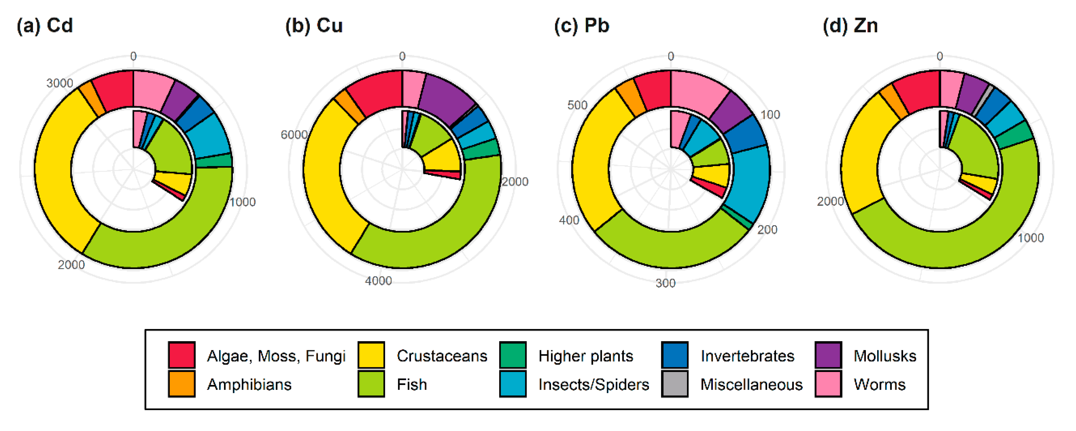
A large amount of toxicity data for the four heavy metals were obtained from the ECOTOX database and a literature search. However, data on Korean resident organisms accounted for less than 35% of the obtained data, which involved an organism reduction of approximately 20–30% (Figure 1). The area in the figure represents the amount of toxicity data for all of the species obtained (outside donut) and Korean species (inside donut), showing the amount of data increasing clockwise from scale 0 on the chart. The colors in the figure show different taxa. The data for Cu were the most abundant, while the data for Pb were significantly less than the other metals. More than half of metal toxicity studies on fish and crustaceans have been conducted, confirming the relative lack of research on other organisms. The resident species notably included less toxicity data on amphibians, higher plants, and mollusks. Many data were also additionally excluded in the process of data screening based on the exposure duration, endpoints, concentration adjustment, and data reliability. After data quality analysis, the remaining data considered available consisted of 48 species for Cd, 55 species for Cu, 26 species for Pb, and 30 species for Zn (

Table 4. Species compositions that comprise the toxicity data for the heavy metals in this study.

Taxonomic Groups	Cd	Cu	Pb	Zn
Algae	1	2	-	-
Crustaceans	15	24	6	13
Fish	7	9	6	6
Insects	4	3	3	3
Invertebrates	11	11	8	4
Mollusks	3	-	-	-
Higher plants	-	2	-	-
Worms	7	4	3	4
Total	48	55	26	30

). These added more species than the previous work [14]. In particular, the addition of insect data contributed to the species diversity for SSDs even though only one genus, Chironomus, was included. It has been controversial whether conventional toxicity tests are suitable for aquatic insects. Poteat and Buchwalter [26] predicted that the metal toxicity of aquatic insects could be different from other organisms in the response duration, toxicity mechanisms, physiological responses, and exposure routes. Mogren and Trumble [27] suggested that the heavy metal toxicity of insects should be observed by focusing on changes in behavior. Despite such issues, aquatic insects are important organisms because they account for a large proportion of freshwater invertebrates in Korea [28]. Little data on plants were obtained. Data for higher plants were available for only Cu, and those for algae were available for Cd and Cu. For Pb and Zn, data for any plants were not available.

According to the Korean government’s data requirements (toxicity data with four taxa including five species and more) and other jurisdictions (for example, toxicity data for different species belonging to eight families in the US, toxicity data for at least 10 species in eight families and more in the EU, and toxicity data at least four taxa including five or more species in Australia and New Zealand), the required species composition was not partially met, but the minimum required data were satisfied. More than half of the toxicity data included species that are widely distributed in the country, so it is expected to reduce some uncertainty of SSDs due to the species composition. Especially, Cd data containing three mollusks (Semisulcospira coreana, Semisulcospira forticosta, and Semisulcospira gotschei) were meaningful because these species are not included in other metal data and live in many freshwater areas in Korea. Cu data, including phytotoxicity, could be used to predict the toxicity of a broader ecosystem. However, Pb and Zn data should be limited to account for animal toxicity only, as there were no plant data.

3.2. Toxicity Data

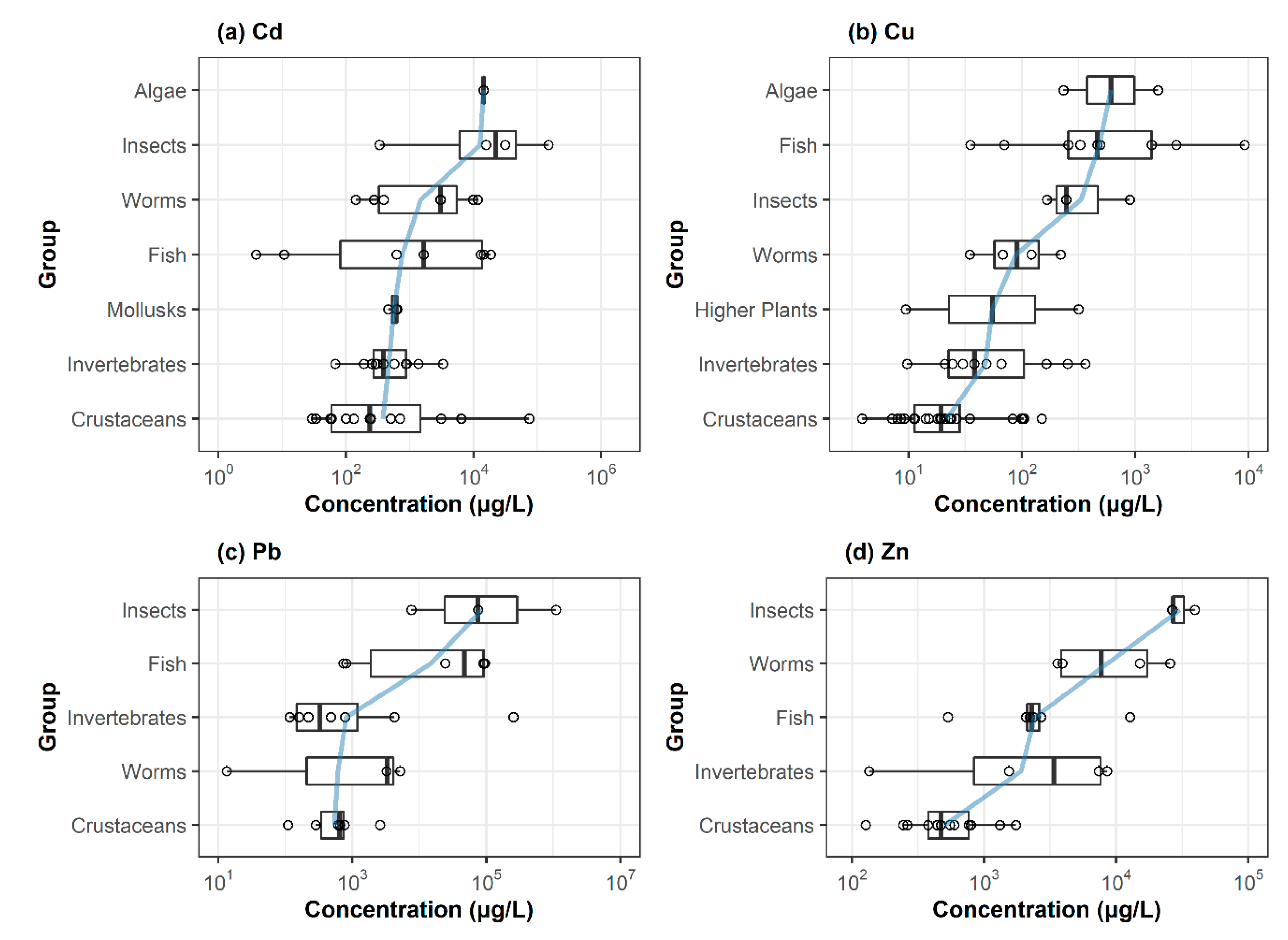
Figure 2 shows concentration ranges based on the toxicity data for heavy metals available for various Korean aquatic species. Toxicity for species and taxa are indicated by points and boxes, respectively, and lines connect the average. Full toxicity values are given in Supplementary Tables S1–S4. In this study, crustaceans tended to be the most sensitive to heavy metals. This was consistent with other studies [29]. In particular, insects tended to be less sensitive to target heavy metals than other animals. The range of distribution was expanded due to some toxicity values of insects.

The range of toxicity data for Cd was from 3.9 to 149,250 μg/L, over four orders of magnitude. Most of the taxa included a wide range of toxicity values, and some ranges appeared concurrently. For example, two fish in the genus Oncorhynchus were the most sensitive to Cd, while the other fish had a toxicity response at concentrations of 100 to 1000 times higher than those of the sensitive fish. Crustaceans, on average, were sensitive to Cd, but the taxa contained the second-highest concentration. Both worms and invertebrates also showed toxicity differences of approximately two orders of magnitude. Three mollusks belonging to the genus Semisulcospira exhibited similar toxicity values and were covered by the toxicity ranges of the other taxa. Algae were less sensitive to Cd, but only one species (Chlorella vulgaris) was considered herein. Versteeg [30] used the standard test organism Pseudokirchneriella subcapitata, which is not a Korean species, to observe the effect of Cd on the population. This study generated a much lower toxicity value in the EC50 range from 120–180 μg/L, suggesting the possibility that algal toxicity may be higher. Therefore, further research is needed to demonstrate the toxicity of algae.

The Cu toxicity data ranged from 3.9 μg/L to over 2000 times starting with Bosmina longirostris. On average, crustaceans were the most sensitive to Cu toxicity, followed by invertebrates, higher plants, worms, insects, fish, and algae. This trend fully explained the concentration range of toxicity data by taxonomic groups. Toxicity data of crustaceans, regarded as the most sensitive taxa, started at the lowest concentration and did not exceed the toxicity range of the next sensitive taxa, invertebrates. It was reasonable for invertebrates containing more toxicity data at lower concentrations to be more sensitive than higher plants even though their toxicity ranges were similar. Fish were less sensitive to Cu and exhibited a wide range of toxicity values.

The metal with the most extensive toxicity data was Pb, with a range between 13.4 μg/L in Tubifex tubifex and 1,096,542 μg/L in Chironomus yoshimatsui. Insects and fish appeared less sensitive than the other three taxonomic groups. Many toxicity data for Pb were available in the toxicity range indicated by invertebrates. Worms included the most sensitive toxicity value, and crustaceans represented a narrow toxicity range. There were no Pb toxicity data available for aquatic plants. For example, Jouany et al. [31] tested resident species (C. vulgaris). They generated acute toxicity values ranging from 530–2200 μg/L, which could be between the toxicity ranges of fish and invertebrates. However, applying these data was limited because hardness adjustment of the toxicity values was not possible. Other Pb toxicity values using non-resident algae were found at lower concentrations in the range of 40–680 μg/L [32].

Compared to other heavy metals, the range of Zn toxicity was narrow and started at a higher concentration. There was a tendency for the average toxicity by taxonomic groups. The most sensitive taxa were crustaceans and followed by invertebrates, fish, worms, and insects. The range of toxicity values for more sensitive taxa did not exceed the range for the next sensitive taxa. Regardless of species habitats or data processing, algal toxicity values for Zn showed a very extensive range from 0.4 to 65,000 μg/L [33,34]. This toxicity range exceeded the toxicity range applied in this study, so further research on algal toxicity is encouraged.

3.3. Species Sensitivity Distribution

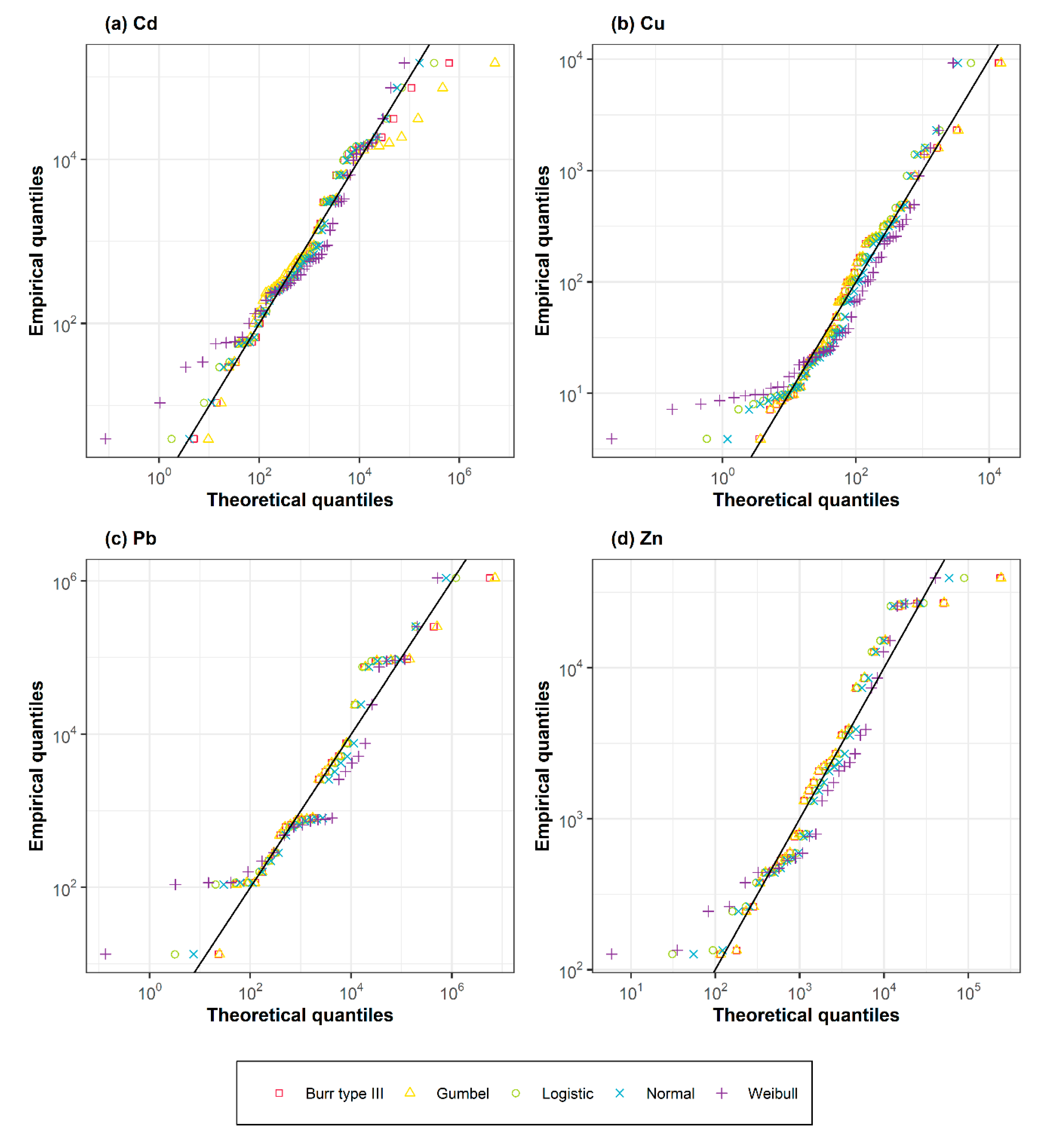
First, the goodness-of-fit was confirmed through AD and KS tests (

Table 5. Goodness-of-fit and information criteria of the SSD models for the four metals.

Heavy Metals	Models	AD a (p value)	KS b (p value)	AIC c
Cd	Burr Type III	0.333 (0.911)	0.079 (0.900)	863.9
	Gumbel	0.519 (0.726)	0.103 (0.648)	865.7
	Logistic	0.459 (0.788)	0.095 (0.740)	862.9
	Normal	0.417 (0.831)	0.107 (0.610)	861.1
	Weibull	1.092 (0.312)	0.157 (0.168)	869.0
Cu	Burr Type III	0.491 (0.755)	0.082 (0.850)	668.7
	Gumbel	0.465 (0.782)	0.080 (0.875)	666.4
	Logistic	0.847 (0.448)	0.106 (0.569)	675.2
	Normal	0.882 (0.425)	0.128 (0.327)	673.8
	Weibull	2.009 (0.091)	0.161 (0.118)	692.3
Pb	Burr Type III	0.360 (0.887)	0.139 (0.696)	536.6
	Gumbel	0.351 (0.895)	0.134 (0.739)	534.7
	Logistic	0.620 (0.628)	0.171 (0.432)	537.2
	Normal	0.641 (0.608)	0.191 (0.301)	535.9
	Weibull	1.050 (0.332)	0.202 (0.240)	541.7
Zn	Burr Type III	0.312 (0.929)	0.084 (0.972)	569.9
	Gumbel	0.309 (0.930)	0.084 (0.973)	567.9
	Logistic	0.495 (0.750)	0.113 (0.798)	570.9
	Normal	0.509 (0.737)	0.125 (0.688)	568.8
	Weibull	0.927 (0.397)	0.134 (0.604)	573.9

^a Anderson-Darling, ^b Kolmogorov-Smirnov, ^c Akaike’s information criterion.

) and Q-Q plots (Figure 3). All of the SSD models were appropriate to represent the heavy metals’ toxicity data. The acceptance of the AD test’s hypothesis supported strong confidence in HC5 because the analysis is more weighted on the distribution tail [8]. Since all of the models considered were identified as correct, the next step was to choose the most suitable model. AIC is a widely used information criterion for selecting the best predictive model. The inconsistency between the true model and the candidate model was quantified. These methods analyze the models’ relative fit by calculating the loss of information in the original data due to the candidate distribution model. The less information loss, the smaller the AIC value, indicating a better fit model [19]. In this study, the most fitted models were the normal distribution for Cd and the Gumbel distribution for the other three metals (Cu, Pb, and Zn). The Weibull distribution showed markedly higher AIC values than the other models, indicating the least suitable model for all of the metals. However, some models demonstrated that the difference between the AIC values was not so substantial. For example, the difference in the models’ AIC values, excluding the Weibull distribution, was approximately 1 for Pb and Zn. In this case, when multiple distributions similarly fit the data, choosing only one of the appropriate models is controversial and ignores information estimated from other deselected models [24]. As an alternative, a weighted average of several models was suggested, which is detailed in the next section.

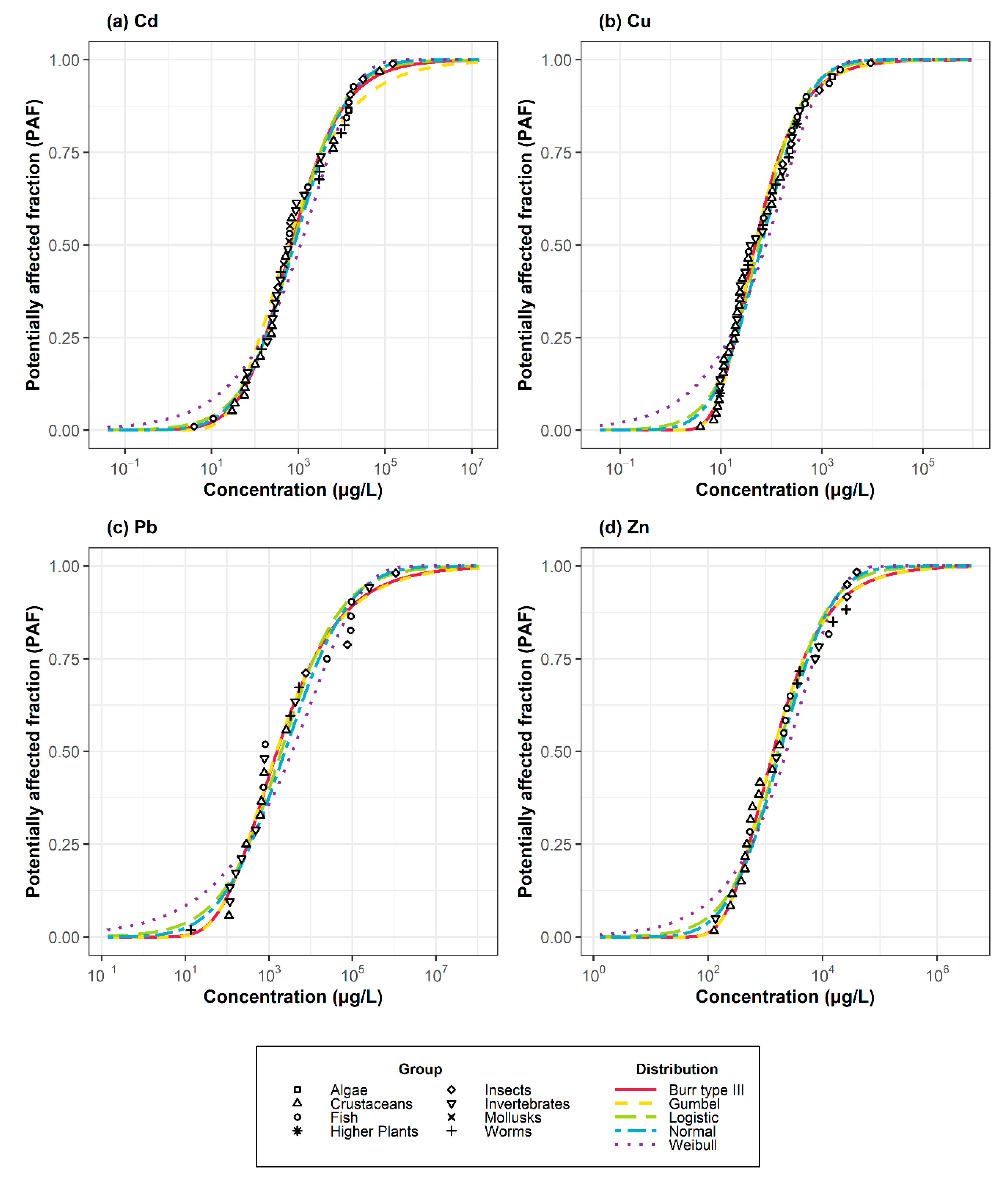
SSDs for heavy metals were depicted based on five distribution models (Figure 4). The points represent the species’ toxicity data and are expressed in multiple shapes representing different taxa. The lines with different colors and types refer to separate model-based SSDs. Through the graphical investigation (Figure 4), an apparent discrepancy between the data and the lower tail in the Weibull distribution was revealed for all of the heavy metals. Cd SSDs excluding the Weibull distribution fully described the data at the lower tails, while in the upper tails, there was a difference in the ability to fit the data according to the models. In particular, the Gumbel distribution stretched the upper tail as it deviated from the data near the top. For Cu SSDs, the Gumbel and Burr Type III models fully described the data in the lower tail compared to the other models. As expected from the AIC results, the AIC values for these two models were similarly low, followed by the AICs for the normal and logistic models after some intervals. Pb SSDs were produced with less predictive models because of the relatively small sample size and wide concentration range. Especially at high concentrations, the models did not display the data well. The models’ lower tails also represented the data poorly. Thus, the HC5 estimation might be accompanied by considerable uncertainty. Zn SSDs were expected to have reduced predictive power at high concentrations. The Burr type III and Gumbel models described the data well at low concentrations, but demonstrated poor prediction at high concentrations. The logistic and normal models showed the opposite trend from the previous two models.

3.4. Predicted No Effect Concentration

The ultimate aim of SSDs is to derive PNEC values for organism protection using a distribution model that adequately describes various toxicity values. Many studies have proven that different PNECs are calculated for different SSD models [3,7]. Therefore, it is necessary to compare not only the model’s fit but also HC5 and PNEC derived from that model. In the previous section comparing SSD models, the Weibull distribution was accepted by the goodness-of-fit hypothesis, but not as good as the other models. The HC5 estimations also resulted in very different values from the results of other models. In addition, as shown in

Table 6. The hazardous concentration of 5% of the species (HC5) and predicted no effect concentration (PNEC) values derived from species sensitivity distribution (SSD), with a 95% confidence interval (CI) in parenthesis.

Heavy Metals	SSD Models	HC5 (μg/L)		CI Ratio	PNEC (μg/L)
		Previous Study	This Study		AF = 2	AF = 5
Cd	Burr type III	-	22.8 (7.9–68.3)	8.7	11.4	4.6
	Gumbel	-	23.8 (12.9–50.8)	3.9	11.9	4.8
	Logistic	-	15.0 (5.0–47.3)	9.0	7.5	3.0
	Normal	14.6 (5.1–47.1)	18.4 (7.5–57.8)	7.7	9.2	3.7
	Weibull	-	3.1 (0.6–18.3)	31.0	1.5	0.6
	Average	-	18.4 (7.2–56.0)	7.8	9.2	3.7
Cu	Burr type III	-	6.7 (4.5–11.4)	2.5	3.3	1.3
	Gumbel	-	6.7 (4.8–10.5)	2.2	3.4	1.4
	Logistic	-	3.2 (1.5–6.5)	4.2	1.6	0.6
	Normal	3.9 (2.0–8.2)	4.0 (2.0–8.4)	4.2	2.0	0.8
	Weibull	-	0.6 (0.1–2.4)	17.0	0.3	0.1
	Average	-	6.6 (4.6–10.6)	2.3	3.3	1.3
Pb	Burr type III	-	47.1 (16.5–230.6)	14.0	23.6	9.4
	Gumbel	-	47.4 (18.7–160.2)	8.6	23.7	9.5
	Logistic	-	15.9 (2.9–113.5)	39.0	8.0	3.2
	Normal	39.2 (9.0–202.8)	24.4 (5.2–143.5)	27.0	12.2	4.9
	Weibull	-	2.1 (0.1–41.4)	367.0	1.1	0.4
	Average	-	37.2 (12.8–160.7)	13.0	18.6	7.4
Zn	Burr type III	-	177.6 (103.8–373.6)	3.6	88.8	35.5
	Gumbel	-	178.1 (107.1–321.8)	3.0	89.1	35.6
	Logistic	-	93.3 (32.1–279.6)	8.7	46.7	18.7
	Normal	133.4 (65.9–301.9)	122.0 (53.3–317.7)	6.0	61.0	24.4
	Weibull	-	35.4 (6.2–177.4)	29.0	17.7	7.1
	Average	-	150.9 (82.0–321.8)	3.9	75.5	30.2

, confidence interval (CI) ratios in which the rate of the upper and lower CI limits were calculated had markedly high values in the Weibull models. The excessively wide CIs indicated considerable uncertainty [35]. Therefore, the Weibull distribution was excluded from consideration. Among the other four models, the logistic distribution derived the most conservative HC5s for all of the heavy metals. Burr type III and Gumbel distributions produced larger HC5s than the logistic and normal distributions and had similar values to each other. The CI was the narrowest in the Gumbel distribution, suggesting a small uncertainty [35]. The HC5s based on normal distributions varied from a previous study [14]. It is not surprising that the results changed due to differences in data usage and data processing methods. In other words, this study supplemented more toxicity data of additional species, removed some outliers within a single species and between multiple species, and differentiated endpoints (e.g., mortality and immobility). This change was intended to reduce and improve the uncertainty of PNECs. The variation acted within the CI of HC5 and demonstrated the uncertainty accompanying AF 2.

The HC5s derived from Cd SSDs were calculated as 15.0–23.8 μg/L, which means 1.6 times the model variability. Based on the AIC values among the Cd SSDs, the normal distribution considered the most suitable model produced an HC5 of 18.4 μg/L with a CI ratio of 7.7. The PNEC with AF 2 was 9.2 μg/L, which was within the CI. It is believed that AF 2 did not sufficiently reflect the model’s uncertainty. The PNEC with AF 5 was calculated much below the lower end of the CI. Thus, AF 3, which was between AF 2 and AF 5, was considered and had a PNEC of 6.1 μg/L. The derived Cd HC5s and PNECs were higher than some water standards in other jurisdictions. For example, it is recommended that Cd concentrations of water at a hardness of 100 mg/L as CaCO₃ are 1.8 μg/L in USEPA [36], 0.9 μg/L in EC [37], and 2.1 μg/L in CCME [38]. For Cu, HC5s of 3.2–6.7 μg/L were derived with a CI ratio of 2.1 by different SSD models. Gumbel and Burr type III distributions representing high suitability derived 6.7 μg/L of HC5 with relatively narrow CIs. Most of the PNECs applied by AF were lower than the CIs of the Cu SSD models. These values were lower than the previous standards in North America, which were 11 μg/L in British Columbia [39] and 14 μg/L in the USA [40]. However, these jurisdictions use the biotic ligand model (BLM) rather than the previous standards. Some research in China induced HC5s comparable to the results of this study, ranging from 2.03–5.13 μg/L [3]. Some organisms from both countries may have contributed. Changes in the SSDs due to species composition have been demonstrated by many studies [41]. HC5s of Pb ranged from 15.9–47.4 μg/L with high CI ratios. A considerable difference between the models was confirmed compared to other heavy metals. The CIs were also more extensive than other heavy metals, probably due to the relatively small sample size. These CIs included the PNECs with AF 2, indicating that the uncertainty due to the model was not sufficiently taken into account. However, PNEC with AF 5 was found to be too conservative. PNECs with different AFs between 2 and 5 may be reasonable to compensate for the model’s uncertainty. Therefore, PNEC with AF 3 was calculated in 15.8 μg/L for Pb. For comparison, the USEPA recommended 65 μg/L as Pb WQC [40], and the European Communities suggested 14 μg/L of Pb EQS-MAC [37]. Xing et al. [3] also used several SSD models to derive Pb HC5s and achieved higher values in the range of 40.9–137.8 µg/L. Zn SSDs induced HC5s in the range of 93.3–178.1 μg/L, with a CI ratio of 3.9. The Gumbel distribution, the best fit out of the Zn SSDs, had 178.1 μg/L of HC5. For the Burr type III and Gumbel distributions, PNECs with AF 2 outside the CI were considered sufficient. The US recommended 120 μg/L as Zn WQC [40], and the UK suggested 50 μg/L as Zn EQS [42] at a hardness of 100 mg/L as CaCO₃.

When several distribution models describe the data similarly, Schwarz and Tillmanns [24] suggested a weighted average HC5. This was a method of allocating and averaging specific weights based on the difference in AIC values for all of the distribution models. As a result, a weight of 0.01 was assigned to the Weibull distribution with the lowest fit and highest AIC value. However, more weights were assigned to the two models with the lowest AIC values, resulting in a weighted average. The CI was expanded over the CI of the most suitable model but was smaller than the CI of the next-best model. This method may avoid the problem of choosing only one model, then generating more stable PNECs with reduced uncertainty.

In general, SSD development and PNEC derivation involve various uncertainties. To reduce such uncertainties, this study focused on elaborate data use and processing and statistical techniques. First, the toxicity data were composed of the resident organisms’ toxic responses. The use of resident species may reflect the ecological environment in Korea. Since the data used affect the accuracy and usefulness of SSDs [12], the available toxicity data were selected according to strict criteria for accuracy, relevance, and reliability. For each species, the most sensitive toxic response was used, except for some outliers. SSDs were developed using several distribution models to determine the best distribution that describes the toxicity data for each heavy metal. The PNECs were derived by considering uncertainty with the application of AF. Nevertheless, uncertainty persists. Conventionally, the SSD is preferably developed with chronic toxicity data, and the acute-to-chronic ratio (ACR) is applied when acute toxicity is used [4]. However, the chronic toxicity data of resident organisms for the heavy metals were not very sufficient in the preliminary study. The application of ACR causes another uncertainty because of the differences in chemicals, species, and experimental conditions [12]. Therefore, this study did not use the ACR but considered the short-term environmental conditions. The underlying assumption of the SSD (for example, the same importance of every species, extrapolation from simple laboratory tests to complex real worlds, and bias of some taxa) may be the leading cause [5,6]. Furthermore, this study concerns the derivation of generic PNECs covering a comprehensive freshwater system in Korea, excluding site-specific environmental parameters and ecosystem conditions. However, when heavy metal exposure occurs in natural waters, it interacts with environmental parameters to change the metal fractions and toxicity to aquatic organisms [43]. For example, metal toxicity is decreased by the complexation of metal ions with organic matters and natural substances in waters, or by the competition between metal ions and cations (e.g., Ca²⁺ and Mg²⁺) composing hardness [44]. This suggests that generic PNECs may be overestimated or underestimated for the risk of specific site. Water effect ratio (WER) may adjust the generic PNEC by comparing the toxicity of water controlled in standard conditions with that of site-specific water [45]. Recently, the biotic ligand model (BLM) has made a great progress for site-specific assessment. BLM assumes that the surface of an organism is a biological ligand that binds metal ion. Metal bioavailability is predicted by the magnitude of the metal ion binding to the biological ligand, and the mechanism that metal ions compete or combine with the environmental parameters is mathematically calculated at specific sites [46]. Therefore, the next challenge is to explore site-specific assessment based on generic PNECs. Besides, it is necessary to explore the environmental concentration of heavy metals in the field to identify ecological risks.

4. Conclusions

In this study, the SSDs for four heavy metals based on Korean resident organisms were developed. Although plant species’ toxicity data were not available for some heavy metals, the minimum amount of data required for the SSDs was satisfied, including the important species. However, it is necessary to add toxic values for plants and species with few data for an accurate comparison. The goodness-of-fit test accepted all five SSD models considered in this study, but the Weibull distribution had difficulty explaining the data at the lower tails. The most suitable models were the normal distribution for Cd and the Gumbel distribution for Cu, Pb, and Zn. There were differences between HC5s and CIs depending on the models, indicating uncertainty due to the models. Based on the CIs, the Gumbel distribution was expected to have a small uncertainty, but the Weibull distribution was expected to have a considerable uncertainty. Pb SSDs had more uncertainty than the other heavy metals, probably due to the relatively small sample size. The PNECs of Cu and Zn derived by AF 2 were 3.4 and 89.1 μg/L, respectively, while the PNECs of Pb and Cd with AF 3 were 6.1 and 15.8 μg/L, respectively. PNEC with AF 5 generated an excessive conservative situation for all of the heavy metals and models. This study reduced some uncertainty by considering the resident species, performing elaborate data processing, identifying the best SSD model for the data, and applying reasonable AFs. In the future, based on this study, it is necessary to investigate the risks of ecosystems to heavy metals in freshwater environments in Korea.

References

- Tchounwou, P.B.; Yedjou, C.G.; Patlolla, A.K.; Sutton, D.J. Heavy metal toxicity and the environment. Exp. Suppl. 2012, 101, 133–164. [Google Scholar] [CrossRef] [PubMed] [Green Version]
- EC. Technical Guidance Document on Risk Assessment in Support of Commission Directive 93/67/EEC on Risk Assessment for New Notified Substances, Commission Regulation (EC) No 1488/94 on Risk Assessment for Existing Substances and Directive 98/8/EC of the European Parliament and of the Council Concerning the Placing of Biocidal Products on the Market; EUR 20418 EN/2; European Commission, Joint Research Centre: Ispra, Italy, 2003. [Google Scholar]
- Xing, L.; Liu, H.; Zhang, X.; Hecker, M.; Giesy, J.P.; Yu, H. A comparison of statistical methods for deriving freshwater quality criteria for the protection of aquatic organisms. Environ. Sci. Pollut. Res. Int. 2014, 21, 159–167. [Google Scholar] [CrossRef] [PubMed]
- Belanger, S.; Barron, M.; Craig, P.; Dyer, S.; Galay-Burgos, M.; Hamer, M.; Marshall, S.; Posthuma, L.; Raimondo, S.; Whitehouse, P. Future needs and recommendations in the development of species sensitivity distributions: Estimating toxicity thresholds for aquatic ecological communities and assessing impacts of chemical exposures. Integr. Environ. Assess. Manag. 2017, 13, 664–674. [Google Scholar] [CrossRef] [PubMed] [Green Version]
- Posthuma, L.; Suter, G.W.; Traas, T.P. Species Sensitivity Distributions in Ecotoxicology; CRC: Boca Raton, FL, USA, 2001. [Google Scholar]
- Smetanová, S.; Bláha, L.; Liess, M.; Schäfer, R.B.; Beketov, M.A. Do predictions from Species Sensitivity Distributions match with field data? Environ. Pollut. 2014, 189, 126–133. [Google Scholar] [CrossRef]
- Newman, M.C.; Ownby, D.R.; Mézin, L.C.A.; Powell, D.C.; Christensen, T.R.L.; Lerberg, S.B.; Anderson, B.-A. Applying species-sensitivity distributions in ecological risk assessment: Assumptions of distribution type and sufficient numbers of species. Environ. Toxicol. Chem. 2000, 19, 508–515. [Google Scholar] [CrossRef] [Green Version]
- Zajdlik, B.A. Potential Statistical Models for Describing Species Sensitivity Distributions; Canadian Council of Ministers of the Environment: Winnipeg, MB, Canada, 2006.
- USEPA. Guidelines for Deriving Numerical National Water Quality Criteria for the Protection of Aquatic Organisms and Their Uses; PB85-227049; United States Environmental Protection Agency: Duluth, MN, USA, 1985.
- ANZECC/ARMCANZ. Australian and New Zealand Guidelines for Fresh and Marine Water Quality; ANZECC/ARMCANZ: Canberra, Australia, 2000. [Google Scholar]
- CCME. A Protocol for the Derivation of Water Quality Guidelines for the Protection of Aquatic Life 2007; Canadian Council of Ministers of the Environment: Winnipeg, MB, Canada, 2007.
- Warne, M.S.J.; Batley, G.E.; van Dam, R.A.; Chapman, J.C.; Fox, D.R.; Hickey, C.W.; Stauber, J.L. Revised Method for Deriving Australian and New Zealand Water Quality Guideline Values for Toxicants; Prepared for the Council of Australian Government’s Standing Council on Environment and Water (SCEW); Information Technology and Innovation: Brisbane, Australia, 2015.
- KMOE. Guidelines on Procedures and Methods for Risk Assessment of Environmental Hazards; Korea Ministry of Environment: Environmental Health Policy Divisions: Sejong City, Korea, 2016; p. 585.
- Park, J.; Lee, S.; Lee, E.; Noh, H.; Seo, Y.; Lim, H.; Shin, H.; Lee, I.; Jung, H.; Na, T.; et al. Probabilistic ecological risk assessment of heavy metals using the sensitivity of resident organisms in four Korean rivers. Ecotoxicol. Environ. Saf. 2019, 183, 109483. [Google Scholar] [CrossRef]
- USEPA. ECOTOX Knowledgebase. Available online: http://cfpub.epa.gov/ecotox/ (accessed on 2 June 2018).
- KMOE. National List of Species of Korea. Available online: http://kbr.go.kr (accessed on 31 December 2017).
- OECD. Report of the OECD Workshop on Extrapolation of Laboratory Aquatic Toxicity Data to the Real Environment; Organisation for Economic Co-operation and Development: Paris, France, 1992. [Google Scholar]
- USEPA. The Metals Translator: Guidance for Calculating a Total Recoverable Permit Limit from a Dissolved Criterion; United States Environmental Protection Agency: Washington DC, USA, 1996; p. 67.
- Akaike, H. A new look at the statistical model identification. IEEE Trans. Autom. Control. 1974, 19, 716–723. [Google Scholar] [CrossRef]
- Dutang, C.; Vincent, G.; Pigeon, M. actuar: An R Package for Actuarial Science. J. Stat. Softw. 2008, 25, 1–37. [Google Scholar]
- Delignette-Muller, M.; Dutang, C. Fitdistrplus: An R Package for Fitting Distributions. J. Stat. Softw. 2015, 64, 1–34. [Google Scholar] [CrossRef] [Green Version]
- Faraway, J.; Marsaglia, G.; Marsaglia, J.; Baddeley, A. goftest: Classical Goodness-of-Fit Tests for Univariate Distributions. R Package Version 1.2-2. Available online: https://CRAN.R-project.org/package=goftest (accessed on 6 August 2020).
- Wickham, H.; Averick, M.; Bryan, J.; Chang, W.; McGowan, L.; François, R.; Grolemund, G.; Hayes, A.; Henry, L.; Hester, J.; et al. Welcome to the Tidyverse. J. Open Source Softw. 2019, 4, 1686. [Google Scholar] [CrossRef]
- Schwarz, C.J.; Tillmanns, A.R. Improving Statistical Methods to Derive Species Sensitivity Distributions; Province of British Columbia: Victoria, BC, Canada, 2019. [Google Scholar]
- Brock, T.C.; Arts, G.H.; Maltby, L.; Van den Brink, P.J. Aquatic risks of pesticides, ecological protection goals, and common aims in european union legislation. Integr. Environ. Assess. Manag. 2006, 2, e20–e46. [Google Scholar] [CrossRef]
- Poteat, M.D.; Buchwalter, D.B. Four reasons why traditional metal toxicity testing with aquatic insects is irrelevant. Environ. Sci. Technol. 2014, 48, 887–888. [Google Scholar] [CrossRef] [PubMed]
- Mogren, C.L.; Trumble, J.T. The impacts of metals and metalloids on insect behavior. Entomol. Exp. Appl. 2010, 135, 1–17. [Google Scholar] [CrossRef]
- Jung, S.W.; Lee, D.H.; Ham, S.A.; Huh, J.M.; Hwang, J.M.; Bae, Y.J. Revised checklist of the Korean aquatic insects. Entomol. Res. Bull. 2011, 27, 37–52. [Google Scholar]
- Yan, Z.; Liu, Z. Toxic Pollutants in China: Study of Water Quality Criteria; Springer: Dordrecht, The Netherlands, 2015; p. 140. [Google Scholar] [CrossRef]
- Versteeg, D.J. Comparison of Short- and Long-Term Toxicity Test Results for the Green Alga. Selenastrum Capricornutum; Wang, W., Gorsuch, J.W., Lower, W.R., Eds.; ASTM International: West Conshohocken, PA, USA, 1990; pp. 40–48. [Google Scholar] [CrossRef]
- Jouany, J.M.; Ferard, J.F.; Vasseur, P.; Gea, J.; Truhaut, R.; Rast, C. Interest of dynamic tests in acute ecotoxicity assessment in algae. Ecotoxicol. Environ. Saf. 1983, 7, 216–228. [Google Scholar] [CrossRef]
- Lin, K.C.; Lee, Y.L.; Chen, C.Y. Metal toxicity to Chlorella pyrenoidosa assessed by a short-term continuous test. J. Hazard. Mater. 2007, 142, 236–241. [Google Scholar] [CrossRef]
- Wren, M.J.; McCarroll, D. A simple and sensitive bioassay for the detection of toxic materials using a unicellular green alga. Environ. Pollut. 1990, 64, 87–91. [Google Scholar] [CrossRef]
- Guanzon, N.G.; Nakahara, H.; Yoshida, Y. Inhibitory Effects of Heavy Metals on Growth and Photosynthesis of Three Freshwater Microalgae. Fish. Sci. 1994, 60, 379–384. [Google Scholar] [CrossRef] [Green Version]
- Cowen, S.; Ellison, S.L. Reporting measurement uncertainty and coverage intervals near natural limits. Analyst 2006, 131, 710–717. [Google Scholar] [CrossRef]
- USEPA. Aquatic Life Ambient Water Quality Criteria Cadmium; EPA 20-R-16-002; United States Environmental Protection Agency: Washington DC, USA, 2016.
- EC. Proposal for a Directive of the European Parliament and of the Council on Environmental Quality Standards in the Field of Water Policy and Amending Directive 2000/60/EC; European Commission: Brussels, Belgium, 2006. [Google Scholar]
- CCME. Canadian Water Quality Guidelines for the Protection of Aquatic Life: Cadmium; Canadian Council of Ministers of the Environment: Winnipeg, MB, Canada, 2014.
- BCMOE. Copper Water Quality Guideline for the Protection of Freshwater Aquatic Life-Technical Report; British Columbia Ministry of Environment and Climate Change Strategy: Victoria, BC, Canada, 2019. [Google Scholar]
- USEPA. Water Quality Criteria Documents for the Protection of Aquatic Life in Ambient Water; EPA-820-B-96-001; United States Environmental Protection Agency: Duluth, MN, USA, 1996.
- Jin, X.; Zha, J.; Xu, Y.; Giesy, J.P.; Wang, Z. Toxicity of pentachlorophenol to native aquatic species in the Yangtze River. Environ. Sci. Pollut. Res. Int. 2012, 19, 609–618. [Google Scholar] [CrossRef]
- Comber, S.D.; Merrington, G.; Sturdy, L.; Delbeke, K.; van Assche, F. Copper and zinc water quality standards under the EU Water Framework Directive: The use of a tiered approach to estimate the levels of failure. Sci. Total. Environ. 2008, 403, 12–22. [Google Scholar] [CrossRef] [PubMed]
- Allen, H.E.; Hall, R.H.; Brisbin, T.D. Metal speciation. Effects on aquatic toxicity. Environ. Sci. Technol. 1980, 14, 441–443. [Google Scholar] [CrossRef] [PubMed]
- Kim, S.D.; Gu, M.B.; Allen, H.E.; Cha, D.K. Physicochemical Factors Affecting the Sensitivity of Ceriodaphnia dubia to Copper. Environ. Monit. Assess. 2001, 70, 105–116. [Google Scholar] [CrossRef] [PubMed]
- USEPA. Interim Guidance on Determination and Use of Water-Effect Ratios for Metals; United States Environmental Protection Agency: Washington DC, USA, 1994.
- Paquin, P.R.; Gorsuch, J.W.; Apte, S.; Batley, G.E.; Bowles, K.C.; Campbell, P.G.C.; Delos, C.G.; Di Toro, D.M.; Dwyer, R.L.; Galvez, F.; et al. The biotic ligand model: A historical overview. Comp. Biochem. Physiol. Part C Toxicol. Pharmacol. 2002, 133, 3–35. [Google Scholar] [CrossRef]
Figure 1.
Donut charts representing the toxicity data for Korean resident organisms (inside donut chart) among all of the data obtained (outside donut chart).
Figure 2.
Comparison of acute toxicity for heavy metals including (a) Cd, (b) Cu, (c) Pb, and (d) Zn among different taxa.
Figure 3.
Quantile–Quantile (Q–Q) plots of the distribution models for (a) Cd, (b) Cu, (c) Pb, and (d) Zn.
Figure 4.
Five species sensitivity distribution (SSD) models of Korean resident species for (a) Cd, (b) Cu, (c) Pb, and (d) Zn.