Dynamic Analysis of Suction Stabilized Floating Platforms

Abstract

The occurrence of parametric resonance due to the time varying behavior of ocean waves could lead to catastrophic damages to offshore structures. A stable structure that could withstand the wave perturbations is quintessential to operate in such a harsh environment. In this work, the authors detail the relevance of a Suction Stabilized Float (SSF) or a Suction Stabilized Floating platform towards such an application. A generic design of a symmetrically shaped float structure along with its inherent stabilization behavior is discussed. Furthermore, the authors extend their prior research on this topic towards modelling the dynamics of SSF and perform stability analysis. The authors demonstrate the dynamical characteristics of SSF analytically using Floquet theory and Normal Forms technique, in this work. Additionally, the simulation results are verified and validated with the numerical methods.

1. Introduction

The application of offshore structures in the oil and gas industry, wind turbines, solar plants is very common. Currently, in most of these applications, the offshore structures are fixed to the seabed with a solid structure that can resist the hydrodynamic forces exerted by the sea waves. However, these fixed bottom structures are economically not feasible for water depth greater than 20 m [1]. However, wind resources, for more than 1TW power generation are estimated in the far off coast of United States, at water depth greater than 30 m [2]. Hence, there is a need to deploy economically feasible floating platforms, that could withstand the hydrodynamic forces due to sea waves and aerodynamic forces due to wind loads at greater water depth. A Suction Stabilized Floating (SSF) platform is an option that would meet these requirements.

The general floating platforms can be classified as: ballast, buoyancy, and mooring lines. Though the platforms can be stabilized using conventional techniques, they all have their own drawbacks [3]. The comparison of various floating platform configurations applicable towards offshore wind turbines are detailed comprehensively in [4] and a Genetic Algorithm based multi-objective design optimization method for these configurations is explained in [5]. Apart from the general platform designs, a barge type floating offshore platform design for the harvesting wind energy was discussed and analyzed in [6]. A review of the column stabilized semisubmersible hulls, types and formation of dry-trees semisubmersible and their comparative advantages along with dynamic behaviour is elucidated in [7]. A platform could remain afloat with the buoyant force exerted on it by the sea. However, in certain applications, it is also required to resist large pitch and roll motions. For example, in case of wind turbines, a large pitching motion would change angle of thrust on the turbine structure and adversely affect its efficiency [8]. The traditional stability analysis of offshore structures were derived from the ship dynamics and were dependent on the righting moment [9]. Many ‘add-on techniques’ such as bilge keel, roll fins and anti-roll tanks to improve the stability of the offshore structures were inspired from ship designs [10]. In general, these stability enhancement techniques resulted in creating or amplifying restoring torque against the roll motions. An SSF platform is designed with an internal vacuum chamber, that maintains a pressure lower than the atmospheric pressure. This suction effect increases the restoring force on the float, thereby resisting roll and pitch disturbances.

Many dynamical analysis and control techniques for various offshore structures have been demonstrated in the past. A hydrodynamic analysis of a vertical slender pile under the influence of wave action was performed and the relationship between the scour process and bed shear stresses were studied analytically and experimentally in [11]. A hydrodynamic analysis and coupled dynamics study of Catenary Anchor Leg Moorings buoys and attached submarine hoses were performed in [12]. In [13], the dynamic response of the platform, bending moment at the base and mooring line tensions were all simultaneously analyzed to validate the significance of mooring configuration on the stability of a submerged offshore wind turbines. A probabilistic approach, including different loading conditions, damage cases and accounting for their occurrences and its effects towards the stability of offshore structures was implemented in [14]. In some applications, multiple individual units are required to function cohesively to serve as a large floating offshore structure. The dynamical analysis of such a structure comprising of multiple semi-submersible modules towards a floating airport was performed using network theory in [15]. The stability characteristics of a hybrid spar design was evaluated analytically and experimentally using a scaled model in [16]. The nonlinear forcing effects and coupling between modes of motions are also required to be modelled to simulate offshore environment [17]. A comprehensive study of various nonlinear hydrodynamic models applicable towards designing an efficient wave energy converters is detailed in [18]. A nonlinear kinematic and hydrodynamic model was utilized for the dynamical analysis of roll, pitch and yaw instabilities and the occurrence of parametric resonance for an axisymmetric spar-buoy structure in [19]. The application of an active control system in a bottle shaped spar to control pitch disturbances is discussed in [20].

The heave motion due to sea waves has been considered as simple harmonic oscillation in many ship dynamical models and aided in analyzing the phenomenon of heave-roll-pitch coupling and parametric resonance [21,22,23,24,25]. Some of the prominent research works for analysing a time periodic systems were using the Hills method [26], the perturbation techniques [27], the averaging methods [28] and the Floquet theory [29]. The application of Hill’s infinite determinants method is applicable only towards identification of stability bounds of the system. The application of perturbation and averaging techniques are limited only to weakly excited systems, due to the requirement of expressing the periodic coefficients in terms of small parameter [30]. The application of Floquet theory converts a linear time periodic system into a time-invariant equivalent system via Lyapunov–Floquet (L-F) transformation. A Lyapunov direct approach in conjunction with fuzzy logic was employed to determine the stability criteria for a Tension Leg Platform (TLP) in [31]. However, for broad applications, the closed form expression of state evolution (known as state transition matrix) is required to derive the fundamental solution matrix [29]. An approximate symbolic form computation of the State Transition Matrix (STM), using Picard iteration and shifted Chebyshev polynomials was performed in [32,33]. The design of a control system towards chaos control using this technique was detailed in [34]. Though the researchers were successful in analyzing and building controllers for multiple time varying systems using these techniques, their application was limited by the requirement of higher order polynomials for better accuracy.

The Normal Forms theory originated from the works by Poincare [35]. The theory was further developed and applied by subsequent researchers [36,37,38,39]. This technique facilitates the analysis of the nonlinear system by incorporating a local transformation (known as near-identity transformation) around a fixed point or equilibrium solution [40] and its applications are comprehensively detailed in [41]. Though the Normal Forms technique has been predominantly used for analysis of nonlinear equations, a mathematical framework on the application for periodic systems was detailed in [42]. In [43], the authors employ the L-F transformation for linear system, to construct a time invariant form, and Normal Forms technique for the nonlinear system. This theory was further applied to nonlinear systems with periodic coefficients by introducing a detuning parameter or a book-keeping parameter [44,45]. Though the use of book-keeping parameters appears to make the formulations using Normal Forms to be convoluted and cumbersome, a direct approach would ease the computations and provide comparable results [46,47].

In this paper, the authors have worked on extending the prior research [48], towards evaluating the dynamical characteristics of SSF. This work encompasses the following objectives:

• Attempt to showcase the similarities between the Floquet theory for time periodic systems and Poincare theory of Normal Forms technique.
• Formulate the mathematical expression for suction stabilization effect for a symmetrically shaped float/platform.
• Derive the equations of motion for the SSF platform by comparing its behavior to ship dynamics.
• Determine the stability bounds from the reduced order heave-roll SSF platform dynamical equations
• Verify and validate the dynamical characteristics of the reduced system by comparing the results with numerical techniques.

In the subsequent section a brief mathematical background of relevant concepts have been provided. Further, a method for direct application of Normal Forms technique towards periodic systems has been included. Later, a detailed insight into the dynamical modelling of the SSF and its model order reduction are added. Furthermore, the comparative results for stability plots, dynamical characteristics and temporal variations supporting the research objectives are incorporated. Finally, the conclusive remarks and key outcomes of the research work are provided.

2. Mathematical Background

A brief background on the mathematical concepts utilized for the dynamical analysis in this work is detailed in the following subsections.

2.1. Floquet Theory

The stability analysis and response of a linear time periodic system are evaluated using the Floquet Theory. Consider a linear dynamical system

$$\dot{\mathbf{x}}=\mathbf{A}\left(t\right)\mathbf{x}$$

(1)

where $\mathbf{x}\in {\mathbb{R}}^n,t\in {\mathbb{R}}^{+},\mathbf{A}\left(t\right)$ is an $n\times n$ periodic matrix with the principal period T. Let $\mathsf{\Phi }\left(t\right)$ be the State Transition Matrix (STM) that satisfies Equation (1) and has the initial condition $\mathsf{\Phi }\left(0\right)=I$. The solution of the Equation (1) can be written as

$$\mathbf{x}\left(t\right)=\mathsf{\Phi }\left(t\right)\mathbf{x}\left(0\right),0\le t\le T$$

(2)

For $t\ge T$, the solution can be calculated by

$$\mathbf{x}(t+mT)=\mathsf{\Phi }\left(t\right){\mathsf{\Phi }}^m\left(T\right)\mathbf{x}\left(0\right),0\le t\le T,m=1,2,3\dots .$$

(3)

where $\mathsf{\Phi }\left(T\right)$ is the Floquet Transition Matrix (FTM) or the Monodromy matrix. The stability criteria for periodic systems depends upon the eigenvalues of $\mathsf{\Phi }\left(T\right)$, called the Floquet multipliers and the system is stable if all the Floquet multipliers lie on or inside the unit circle, other wise it is unstable.

According to the Lyapunov–Floquet theorem, the STM can be expressed as

$$\mathsf{\Phi }\left(t\right)=\mathbf{Q}\left(t\right)e^{\mathbf{R}t},\mathbf{Q}\left(t\right)\in {\mathbb{R}}^{n\times n},\mathbf{R}\in {\mathbb{R}}^{n\times n},\forall t\ge 0$$

(4)

where $\mathbf{Q}\left(t\right)$ is known as the L-F transformation matrix. The transformation of the time periodic linear matrix to a constant one is accomplished via the L-F transformation, $\mathbf{x}=\mathbf{Q}\left(t\right)\mathbf{y}$. Elements of the L-F transformation matrix $\mathbf{Q}\left(t\right)$ contain truncated Fourier series representation [49]. Applying the L-F transformation to Equation (1) results in Equation (5) with a time-invariant linear part.

$$\begin{array}{cc}\hfill \dot{\mathbf{y}}=& \mathbf{R}\mathbf{y}\hfill \end{array}$$

(5)

where $\mathbf{R}$ is a constant $n\times n$ matrix that generally tends to be complex. The eigenvalues of the $\mathbf{R}$ are known as the Floquet Exponents, that could also be used as an indicator for the stability of dynamical system.

2.2. State Augmentation

The intuitive state augmentation converts the periodic term into a state variable. This approach could be applied to periodic coefficients or periodic external forcing terms. For the ease of understanding, let us consider a time periodic system given by Equation (1), which is modified as Equation (6)

$$\dot{\mathbf{x}}=({\mathbf{B}}_{\mathbf{0}}+\mathbf{B}\left(t\right))\mathbf{x}$$

(6)

where ${\mathbf{B}}_{\mathbf{0}}\left(t\right)$ is the constant matrix, $\mathbf{x}$ is the vector containing the system states and $\mathbf{B}\left(t\right)\mathbf{x}$ is the $n\times 1$ vector containing the periodic coefficients as shown below

$$\mathbf{B}\left(t\right)\mathbf{x}=\left[\begin{array}{c}{B}_1{g}_1\left(t\right)x_1\\ B_2{g}_2\left(t\right)x_2\\ ⋮\\ B_i{g}_i\left(t\right)x_i\end{array}\right],i=1,2,3,\dots .,n$$

(7)

where $B_i$ is the amplitude of the forcing term and $g_i\left(t\right)$ represents a sine or cosine trigonometric function of ${\omega }_i$, i.e., $sin\left({\omega }_{i}t\right)$ or $cos\left({\omega }_{i}t\right)$. The states are augmented as follows

$$\left.\begin{array}{cc}\hfill p_1& =g_1\left(t\right)\hfill \\ \hfill p_2& =g_2\left(t\right)\hfill \\ \hfill ⋮\\ \hfill p_n& =g_n\left(t\right)\hfill \\ \\ \hfill {\dot{p}}_1& =\mp {\omega }_1{\dot{g}}_1\left(t\right)=q_1\hfill \\ \hfill {\dot{p}}_2& =\mp {\omega }_2{\dot{g}}_2\left(t\right)=q_2\hfill \\ \hfill ⋮\\ \hfill {\dot{p}}_n& =\mp {\omega }_n{\dot{g}}_n\left(t\right)=q_n\hfill \\ \\ \hfill {\dot{q}}_1& =-{\omega }_1^2{g}_1\left(t\right)=-{\omega }_1^2{p}_1\hfill \\ \hfill {\dot{q}}_2& =-{\omega }_2^2{g}_2\left(t\right)=-{\omega }_2^2{p}_2\hfill \\ \hfill ⋮\\ \hfill {\dot{q}}_n& =-{\omega }_n^2{g}_n\left(t\right)=-{\omega }_n^2{p}_n\hfill \end{array}\right\}$$

(8)

Hence the augmented $l\times 1$ state vector is given by

$$\tilde{\mathbf{x}}={\left[\mathbf{x},p_1,p_2,\cdots ,p_n,q_1,q_2,\cdots ,q_n\right]}^T$$

(9)

The linear time periodic system gets converted to nonlinear state augmented time invariant system, as the periodic term expressed as states is part of the nonlinear vector in the form indicated in Equation (10).

$$\tilde{\mathbf{B}}\left(\tilde{\mathbf{x}}\right)=\left[\begin{array}{c}{B}_1\breve{f}(\mathbf{x},p_1,p_2,\dots ,p_n,q_1,q_2,\dots ,q_n)\\ B_2\breve{f}(\mathbf{x},p_1,p_2,\dots ,p_n,q_1,q_2,\dots ,q_n)\\ ⋮\\ B_n\breve{f}(\mathbf{x},p_1,p_2,\dots ,p_n,q_1,q_2,\dots ,q_n)\\ 0\\ 0\\ 0\\ 0\\ ⋮\\ 0\\ 0\end{array}\right],n=3,4,\dots$$

(10)

With the state augmentation the Equation (6) is updated as

$$\dot{\tilde{\mathbf{x}}}={\tilde{\mathbf{B}}}_0\tilde{\mathbf{x}}+\tilde{\mathbf{B}}\left(\tilde{\mathbf{x}}\right)$$

(11)

where ${\tilde{\mathbf{B}}}_0$ is a $l\times l$ constant matrix and $\tilde{\mathbf{B}}\left(\tilde{\mathbf{x}}\right)$ is a $l\times 1$ vector containing the augmented nonlinear monomial terms in $\tilde{\mathbf{x}}$. The Equation (11) could be subjected to a modal transformation and the Normal Forms technique could be applied to eliminate the non resonant nonlinear terms. A detailed implementation of the state augmentation along with normal forms technique, for nonlinear systems with periodic forcing terms, are discussed in detail in our prior work [46].

2.3. Normal Forms

The Normal Forms technique aids in eliminating many non-resonant nonlinear terms by employing a near-identity transformation on the system equations [40]. Consider a nonlinear dynamical system given by Equation (12).

$$\dot{\mathbf{x}}=\mathbf{A}\mathbf{x}+\mathbf{F}\left(\mathbf{x}\right)$$

(12)

where $\mathbf{A}$ is a constant $n\times n$ matrix and $\mathbf{F}\left(\mathbf{x}\right)$ is a $n\times 1$ vector containing the nonlinear monomials in $\mathbf{x}$. After applying the modal transformation $\mathbf{x}=\mathbf{M}\mathbf{z}$ to Equation (5), the Jordan canonical form is obtained as shown in Equation (13)

$$\dot{\mathbf{z}}=\mathbf{Jz}+{\mathbf{M}}^{-1}\mathbf{F}\left(\mathbf{z}\right)$$

(13)

where $\mathbf{J}$ is the Jordan form of $\mathbf{A}$ and $\mathbf{M}$ is the modal transformation matrix. The diagonal elements of $\mathbf{J}$ matrix contain the semi-simple eigenvalues of the linear matrix $\mathbf{A}$.

$$\mathbf{J}=\left[\begin{array}{c}\begin{array}{cc}{\lambda }_1& \\ & {\lambda }_2\\ & & \ddots \\ & & & {\lambda }_n\end{array}\end{array}\right]$$

(14)

the system shown in Equation (13) is amenable to an application of Time Independent Normal Forms, which is similar in principal to the averaging technique [28]. A near identity transformation (of the form Equation (15)) is applied to Equation (13)

$$\dot{\mathbf{z}}=\mathbf{v}+{\mathbf{h}}_r\left(\mathbf{v}\right)$$

(15)

where ${\mathbf{h}}_r\left(\mathbf{v}\right)$ is homogenous vector of monomials in $\mathbf{v}$ of r degree. The general homological equation obtained by elimination of higher order nonlinearities is shown as

$$\frac{\partial {\mathbf{h}}_r\left(\mathbf{v}\right)}{\partial \mathbf{v}}\mathbf{Jv}-{\mathbf{Jh}}_r-{\mathbf{F}}_r\left(\mathbf{v}\right)=0$$

(16)

where ${\mathbf{F}}_r\left(\mathbf{v}\right)$ is expressed in terms of solutions of homological equation of order $r-1$, for $r>3$. An approximate solution to Equation (16), can be expressed as

$$\left.\begin{array}{cc}\hfill & {\mathbf{h}}_r\left(\mathbf{v}\right)=\sum _{j=1}^n\sum _{{\mathbf{m}}_r}{h}_{r,j,{\mathbf{m}}_r}{\left|\mathbf{v}\right|}^{{\mathbf{m}}_r}{\mathbf{e}}_j,\hfill \\ \hfill & {\mathbf{F}}_r\left(\mathbf{v}\right)=\sum _{j=1}^n\sum _{{\mathbf{m}}_r}{F}_{r,j,{\mathbf{m}}_r}{\left|\mathbf{v}\right|}^{{\mathbf{m}}_r}{\mathbf{e}}_j\hfill \end{array}\right\}$$

(17)

where ${\mathbf{m}}_r=(m_1,m_2,\dots ,m_n)$, ${\displaystyle \sum _{i=1}^n}{m}_i=r$, $(r=2,3,\dots ,k)$, ${\mathbf{e}}_j$ is the $j^{th}$ member of the natural basis and ${\left|\mathbf{v}\right|}^{{\mathbf{m}}_r}={{\mathbf{v}}_1}^{m_1}{{\mathbf{v}}_2}^{m_2}\dots .{{\mathbf{v}}_n}^{m_n}$. After substituting Equation (17) in Equation (16) and equating the coefficients of similar terms result in

$$h_{r,j,{\mathbf{m}}_r}=\frac{F_{r,j,{\mathbf{m}}_r}}{{\mathbf{m}}_r.\mathsf{\Lambda }-{\lambda }_j}$$

(18)

where $\mathsf{\Lambda }={\left[{\lambda }_1,{\lambda }_2,{\lambda }_3\dots {\lambda }_n\right]}^T$ are the eigenvalues of $\mathbf{A}$. The coefficients of $r^{th}$ order near-identity can only be obtained if the following solvability condition is satisfied.

$${\mathbf{m}}_r.\mathsf{\Lambda }-{\lambda }_j\ne 0$$

(19)

The resonant nonlinear terms would remain in the near identity transformations and Equation (16) gets updated as

$$\dot{\mathbf{v}}=\mathbf{Jv}-\sum _{r=2}^k{\mathbf{F}}_r^{*}\left(\mathbf{v}\right)$$

(20)

where ${\mathbf{F}}_r^{*}\left(\mathbf{v}\right)$ comprises of the resonant terms.

2.4. Direct Application of the Normal Forms Approach

Consider a linear time periodic system with both constant and periodic coefficients, but without external excitation. The Equation (1) can be updated as follows

$$\dot{\mathbf{x}}\left(t\right)=\mathbf{A}\left(t\right)\mathbf{x}\left(t\right)$$

(21)

where $\mathbf{A}\left(t\right)={\mathbf{B}}_0+\mathbf{B}\left(t\right)$. By applying the L-F transformation directly on this system, as mentioned in Section 2.1 converts it into a time-invariant system as shown below, in Equation (22)

$$\dot{\mathbf{y}}\left(t\right)=\mathbf{R}\mathbf{y}\left(t\right)$$

(22)

The solution to Equation (22) can be expressed as

$$\mathbf{y}\left(t\right)=e^{\mathbf{R}t}\mathbf{y}\left(0\right)$$

(23)

Instead of the L-F transformation, if we were to augment the periodic terms, the original system Equation (21), it gets updated in the form of Equation (11), as mentioned in Section 2.2. The updated system has a constant linear part (${\tilde{\mathbf{B}}}_0$) and nonlinear part ($\tilde{\mathbf{B}}\left(\tilde{\mathbf{x}}\right)$ ), as shown in Equation (11). A modal transformation on the updated system, $\tilde{\mathbf{x}}\left(t\right)=\tilde{\mathbf{M}}\tilde{\mathbf{z}}\left(t\right)$, would get the system updated as

$$\dot{\tilde{\mathbf{z}}}=\tilde{\mathbf{J}}\tilde{\mathbf{z}}+{\tilde{\mathbf{M}}}^{-1}\tilde{\mathbf{B}}\left(\tilde{\mathbf{z}}\right)$$

(24)

where $\tilde{\mathbf{M}}$ is the modal transformation matrix and $\tilde{\mathbf{J}}$ is the Jordan form of ${\tilde{\mathbf{B}}}_0$, which contains the semi-simple eigenvalues of both the original states and the augmented states, as shown below in Equation (25).

$$\tilde{\mathbf{J}}=\left[\begin{array}{c}{\lambda }_1\\ & {\lambda }_2\\ & & \ddots \\ & & & {\lambda }_n\\ & & & & {\lambda }_{n+1}\\ & & & & & {\lambda }_{n+2}\\ & & & & & & \ddots \\ & & & & & & & {\lambda }_l\end{array}\right]$$

(25)

At this point, since Equation (24) is in the Jordan form with semi-simple eigenvalues, we could apply a near-identity transformation (Equation (15)) and the Normal Forms technique, as indicated in Section 2.3. It is noted that in this particular case one has to find higher order normal form than the order of the nonlinearity (i.e., two) and then replace the fictitious/augmented states by their closed form expressions (cf. Equation (8)). In case of no resonance, the Normal Forms solution would result in a time-invariant system.

The near identity transformation, at this point would contain the dynamics due to both the system states and the augmented states. The near identity transformation of the reduced state can also be expressed as

$$\tilde{\mathbf{z}}\left(t\right)=\tilde{\mathbf{P}}\tilde{\mathbf{v}}\left(t\right)$$

(26)

where $\tilde{\mathbf{P}}$ serves as the near-identity transformation matrix and contains all the higher order nonlinear terms/coefficients associated with the states and it converts the system in Equation (24) into a linear time-invariant system, as follows

$$\dot{\tilde{\mathbf{v}}}=\tilde{\mathbf{J}}\tilde{\mathbf{v}}$$

(27)

It can be summarized that once the augmented states are replaced by the known temporal terms, the near-identity transformation (in Normal Forms technique), essentially serves as a L-F transformation and converts the linear time variant system to a linear time-invariant system (Equation (27)). It is observed that it is identical to Equation (20), considering the resonant terms are absent. At this point, the augmented states are back substituted into the Normal Forms solution and the matrix becomes a function of time. As indicated in Equation (4), by applying the L-F transformation, the STM of the Normal Forms solution can be expressed as

$$\tilde{\mathsf{\Phi }}\left(t\right)=\tilde{\mathbf{P}}\left(t\right)e^{\tilde{\mathbf{J}}t}$$

(28)

As indicated in Section 2.1, at t=T, the FTM of the reduced system is obtained and the stability plots are generated based on the conditions on the Floquet multipliers and Floquet exponents. Since the reduced system would preserve the dynamical characteristics of the original system, the transition curves would resemble that from the stability analysis of the original system.

It is also noted that using this technique we could also obtain the closed form expression for STM of the reduced system ($\tilde{\mathsf{\Phi }}\left(t\right)$) and thereby that of the original system, $\widehat{\mathsf{\Phi }}\left(t\right)$, using back transformation. This would aid in predicting the state evolution of the original system over time in a closed form.

3. Suction Stabilized Floating Platform

A SSF platform, or Suction-Stabilized Float comprises of an internal chamber maintaining a pressure lower than the atmospheric pressure. This pressure differential results in a suction effect that increases the restoring torque on the float/platform and resists perturbations in roll and pitch motions. This behavior qualifies SSF as an ideal addition for offshore structures.

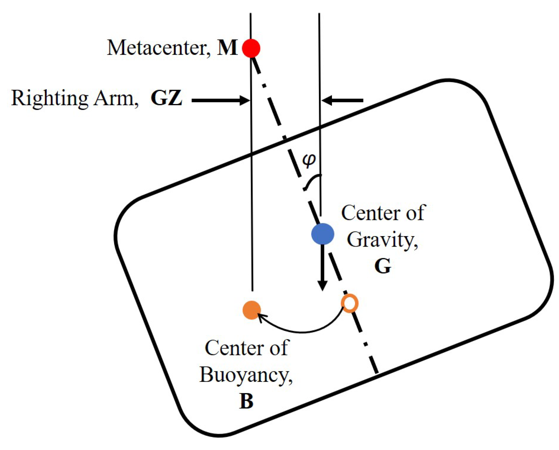
The stability analysis of offshore structures are majorly derived from ship hydrostatics and hydrodynamics [10]. The metacentric height and righting lever are the key paramters, that guide the stability of ship models. For small heel angles, the metacenter being vertically above the center of gravity ensures stability [10]. For large heel angles, the righting moment generated due to the coupling forces of weight of the ship and buoyant force on the ship is used as the criteria of stability [9]. The righting moment of a ship can be expressed as,

$$M_R=W_{ship}\times \overline{GZ}$$

(29)

where $W_{ship}$ is the weight of the ship, $M_R$ is the righting moment, and $\overline{GZ}$ is the horizontal distance between center of buoyancy and center of gravity of the ship, as shown in Figure 1. The value of righting moment majorly depends on $\overline{GZ}$ and for small heel angles, the righting lever is calculated using the metacentric height, as shown in Equation (30) [9].

$$\overline{GZ}=\overline{GM}sin\varphi$$

(30)

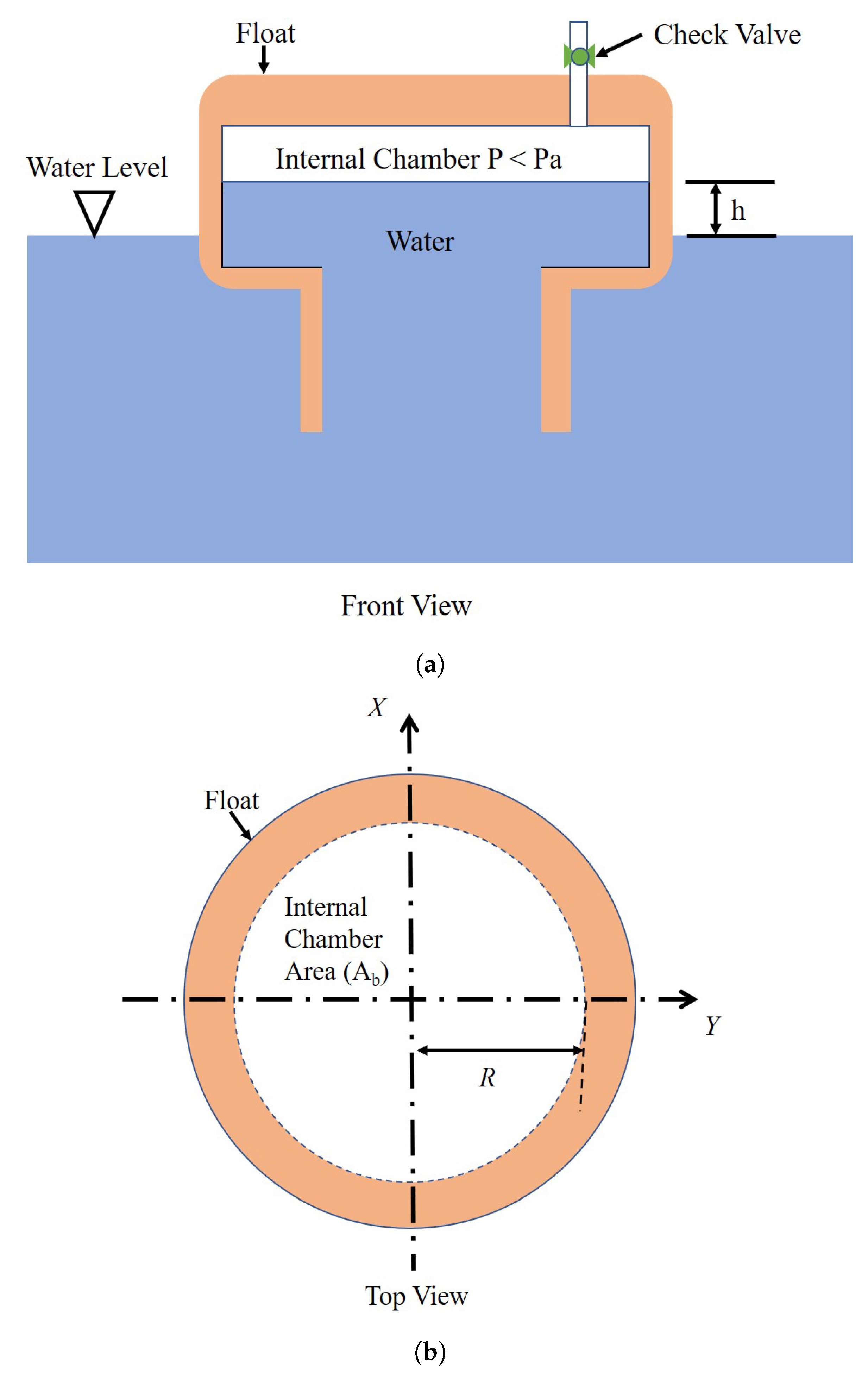
Consider a circular shaped SSF platform, as shown in Figure 2, with an internal chamber of radius R. Using a vacuum pump, connected to the internal chamber via a check valve the vacuum is created in internal chamber. The pressure inside the internal chamber is less than the atmospheric pressure ($P<Pa$). Due to the pressure differential, the water level inside the internal chamber rises by $h=\frac{Pa-P}{\rho g}$(where g is the acceleration due to gravity and $\rho$ is the density of the water). In the equilibrium position, the resolution of forces in the vertical direction is given by

$$(P_a-P)A_b+V_{b}g\rho =Mg$$

(31)

where M is the total mass of the float and $V_b$ is the displaced volume. Since the surface effect of air cushion is present, a direct application of Archimedes law is not feasible. However, Equation (31) is similar to the weight balance equation of a surface effect ship, such as hovercraft, riding on an air cushion [50]. However the internal chamber of the surface effect ships contains positive pressure (above atmospheric pressure) and that of SSF platforms have negative pressure (below atmospheric pressure). Moreover, the air cushion in surface effect ships decreases the metacentric height and righting lever thereby resulting in a destabilizing effect [50]. Whereas, the vacuum in SSF platform increases the metacentric height and righting lever. The equation for righting lever for the SSF platform is derived using the approach presented in [50].

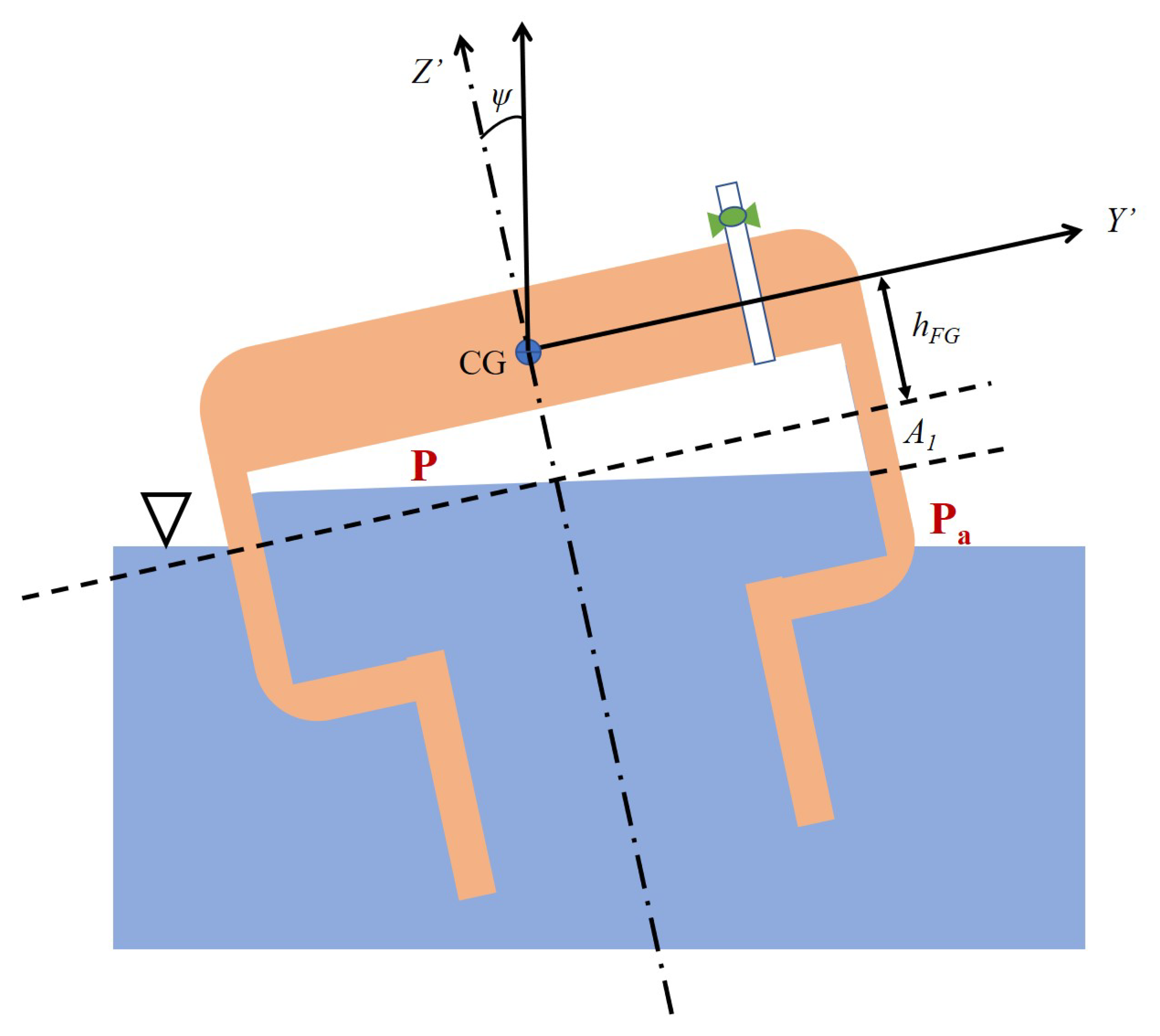
Consider the circular SSF platform heeled by an angle $\psi$, with respect to the vertical, as shown in Figure 3. The atmospheric pressure, outside the platform, is indicated by $P_a$ and that inside the internal chamber is indicated by P. As the platform heels, the area $A_1$ appears outside the water on the right side and an equal area (due to symmetry) disappears into the water on the left side. A differential pressure of $P_0=P_a-P$ acts on the area $A_1$, resulting in a force in the negative Y’ direction and is represented by

$$F_{A_1}=P_0\times A_1$$

(32)

The restoring moment due to this force in the clockwise direction is given by

$$M_{A_1}=h_{FG}\times P_0\times A_1$$

(33)

The cylindrical wedge section generated due to the heel angle represents a cylindrical hoof and the lateral surface area is given by $A_1=2R{h}_{wedge}$ [51]. For the given tilted SSF (where $h_{wedge}=Rtan\psi$), the moment equation can be updated as

$$M_{A_1}=h_{FG}\times P_0\times 2\times R\times Rtan\psi$$

(34)

Similar moment is obtained when the SSF platform heels in the clockwise direction. Due to the symmetrical shape and restoring action, the total moment is represented by

$$\begin{array}{cc}\hfill M& =2\times M_{A_1}\hfill \\ \hfill & =4\times h_{FG}\times P_0\times R^{2}tan\psi \hfill \end{array}$$

(35)

For small heel angles, $tan\psi \approx \psi$, thereby reducing the total restoring moment due to suction stabilization effect as

$$M=4h_{FG}{P}_0{R}^2\psi$$

(36)

It is observed from Equation (36) that the restoring moment is opposite to the direction of heel and is proportional to the heel angle, $\psi$. This effect of suction stabilization can be represented as a torsional spring of stiffness, $k_t$, attached to the CG and can be equated to

$$k_t=4h_{FG}{P}_0{R}^2$$

(37)

Considering conservatively ($4\approx \pi$), the torsional stiffness can also be approximated to

$$k_t\approx h_{FG}{P}_0\pi R^2=h_{FG}{P}_0{A}_b$$

(38)

where $A_b$ is the cross-sectional area of the internal chamber. The effectiveness of this torsional spring in stabilizing the SSF platforms are evaluated in the subsequent sections.

3.1. Dynamical Model for SSF

As detailed in our prior work [48], the dynamical model of SSF was inspired from the ship dynamical models. Similar to the ship motions in sea, the SSF also experiences heave and pitch actions directly. The periodic variation of hull geometry leading to periodic variation of water plane area and thereby resulting in periodic variation of metacentric height. A transfer of energy is observed from the heave motions into roll motions. However, due to the energy transfer and the occurrence of parametric resonance, the roll motions are developed and amplified in certain range of frequencies of sea wave [52,53,54,55].

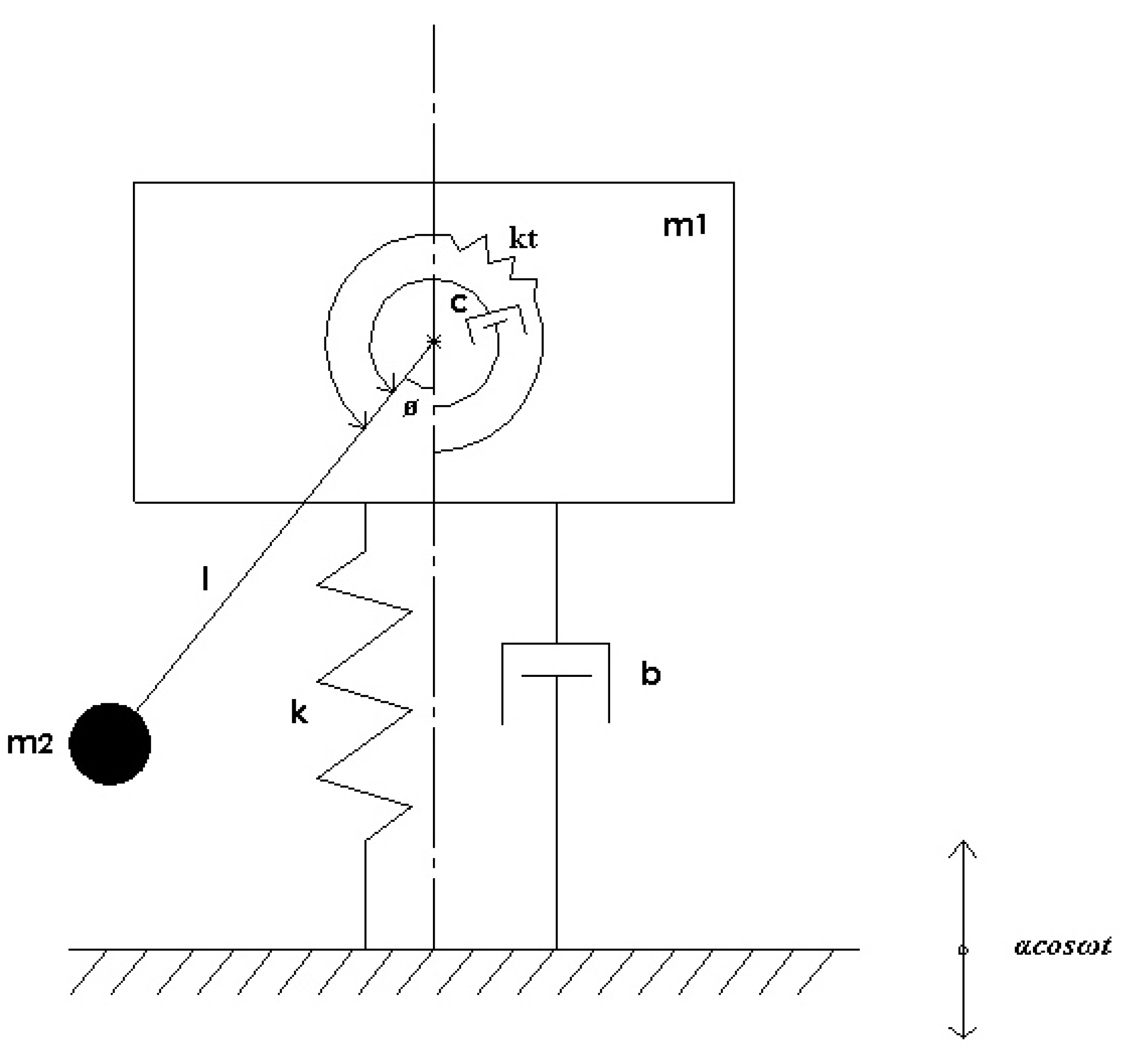
The dynamical behavior of ship motions are investigated using a heave-roll model [52,53,56]. In this model, the ships are subjected to a vertical displacement, under the influence of moderate longitudinal waves, and the stability characteristics under the coupled action of heave and roll motions are studied. Since the properties of ship and SSF platform are comparable, the heave-roll model for ships or floating platform models with cranes [57], are modified to incorporate the restoring torque due to suction stabilization and is indicated in Figure 4.

As shown in Figure 4, the vertical motion of mass $m_1$ (corresponding to vertically displacing mass of ship/platform) represents the heave motion and the pendulum action of the rotating mass $m_2$ (corresponding to rotating mass of ship/platform) represents the roll motion. The linear and rotational damping co-efficients are denoted by b and c, respectively. The length of the pendulum is represented by l, which rotates with an angular displacement $\varphi$. A linear spring of stiffness k is connected between the mass $m_1$ and base of the system. Additionally, a rotational/torsional spring of stiffness, $k_t$, representing the suction stabilization effect, is added to the model. The base of the system experiences a periodic wave motion $\alpha cos\omega t$, where $\omega$ is the frequency of the wave motion. The vertical displacement of the SSF platform is identified by z and roll angle by $\varphi$. The equations of motion for the SSF platform is derived using the Lagrangian method and is outlined in Appendix A.

$$(m_1+m_2)\{\ddot{z}-\alpha {\omega }^{2}cos\left(\omega t\right)\}+b\dot{z}+kz+m_{2}l\{\ddot{\varphi }sin\varphi +{\dot{\varphi }}^{2}cos\varphi \}=0$$

(39)

$$m_2{l}^2\ddot{\varphi }+c\dot{\varphi }+k_t\varphi +m_{2}glsin\varphi +m_{2}l\{\ddot{z}-\alpha {\omega }^{2}cos\left(\omega t\right)\}sin\varphi =0$$

(40)

The equations of motion are simplified for the dynamical analysis in the subsequent subsection.

3.2. Analysis of SSF Model Dynamics

The equations of motion of SSF represented in Equations (39) and (40) are dependent on the geometrical properties. The equations are transformed in the dimensionless form to evaluate the effectiveness of the suction stabilization effect. The dimensionless form is indicated as follows

$$\ddot{x}+\overline{B}\dot{x}+q^{2}x+\mu \{\ddot{\varphi }sin\varphi +{\dot{\varphi }}^{2}cos\varphi \}=a{\eta }^{2}cos\left(\eta \tau \right)$$

(41)

$$\ddot{\varphi }+\overline{C}\dot{\varphi }+sin\varphi +q_t^2\varphi +\{\ddot{x}-a{\eta }^{2}cos\left(\eta \tau \right)\}sin\varphi =0$$

(42)

The semi-trivial solution of Equations (41) and (42) are represented as

$$x_0\left(\tau \right)=a(Mcos\left(\eta \tau \right)+Nsin\left(\eta \tau \right))$$

(43)

$${\varphi }_0\left(\tau \right)=0$$

(44)

where $M=\frac{{\eta }^2(q^2-{\eta }^2)}{{(q^2-{\eta }^2)}^2+{\left(\overline{B}\eta \right)}^2}$ and $N=\frac{\overline{B}{\eta }^3}{{(q^2-{\eta }^2)}^2+{\left(\overline{B}\eta \right)}^2}$. By adding small perturbations to x and $\varphi$ as

$$x=x_0+s$$

(45)

$$\varphi ={\varphi }_0+\theta$$

(46)

By applying first order approximations to Equations (43) and (44), we get

$$\ddot{s}+\overline{B}\dot{s}+q^{2}s=0$$

(47)

$$\ddot{\theta }+\overline{C}\dot{\theta }+(1+q_t^2)\theta -a{\eta }^2\{(1+M)cos\left(\eta \tau \right)+Nsin\left(\eta \tau \right)\}\theta =0$$

(48)

The Equation (47) will generate stable solutions, since it is homogeneous differential equation with constant coefficients. However, Equation (48) is a damped Mathieu equation and its stability bounds are based on the system parameters. It is noted that Equation (48) preserves all the system parameter pertaining to the SSF model. The system parameters ($\overline{B}$ and $q^2$) of the heave motions (from Equation (47)) are also observed to appear in Equation (48). Hence the analysis of reduced order roll motion consolidates the dynamical behavior of the SSF system model.

For the cases with a really low linear damping term $\overline{B}$ and rotational damping term $\overline{C}$, the value of N is negligible, thereby eliminating any terms multiplied by them. Additionally, the $(1+q_t^2)$ term can be replaced with $\delta$ and the $a{\eta }^2(1+M)$ term with $2ϵ$, thereby updating the Equation (48) as follows

$$\ddot{\theta }+(\delta -2ϵcos\left(\eta \tau \right))\theta =0$$

(49)

The Equation (49) is the standard Mathieu equation when $\eta =2$ and could be analyzed using the Floquet theory. It is also feasible to use the direct application of the Normal Forms approach (detailed in Section 2.4), by representing the periodic term as augmented state. However, for the cases with significant linear damping term $\overline{B}$, the value of N is significant and Equation (48) can be updated as follows

$$\ddot{\theta }+\overline{C}\dot{\theta }+(\widehat{\delta }-\widehat{ϵ}\{\frac{cos\left(\eta \tau \right)}{N}+\frac{sin\left(\eta \tau \right)}{(1+M)}\})\theta =0$$

(50)

where $\widehat{\delta }=(1+q_t^2)$ would still be the linear constant term and $\widehat{ϵ}=a{\eta }^2(1+M)N$ will be the coefficient of periodic forcing term. As detailed in our prior work [48], the generic solution for Mathieu equation can be substituted in Equation (48) and solve for the non-trivial solutions for the constant coefficients to derive the expression for threshold amplitude. However, in this work, the system equations are analyzed using the Floquet theory and Normal Forms techniques analytically and results are discussed in the subsequent sections.

4. Materials

All the analytical simulations were performed, and stability plots were generated on a laptop computer (Intel Core i7-7500U CPU 2.90GHz, 16 GB RAM) using MATHEMATICA. The stability plots were generated using Floquet theory and the numerical integration results. The Normal Form solution for the equation with nonlinear terms were determined using the MATHEMATICA package [58].

5. Simulation Results

The reduced order expressions for the SSF dynamical model, from Section 3.2, are studied analytically and evaluated for stability. The linear damping and linear stiffness is attributed towards the heave motion due to the sea waves. The reduced order SSF model with negligible linear damping (Equation (49)) is eligible to be evaluated using both Normal Forms technique and Floquet theory. The transition curves between the stable and unstable region are obtained analytically and plotted. Further, for the case of SSF system with significant linear damping, the stability plots are generated using the Floquet theory on the system Equation (50). In both cases, the parameter in the horizontal coordinate is attributed to the suction stabilization effect. The temporal variations of the system states are plotted in each case to validate the stability behavior obtained.

5.1. SSF with Negligible Linear Damping ($\overline{B}\approx 0$)

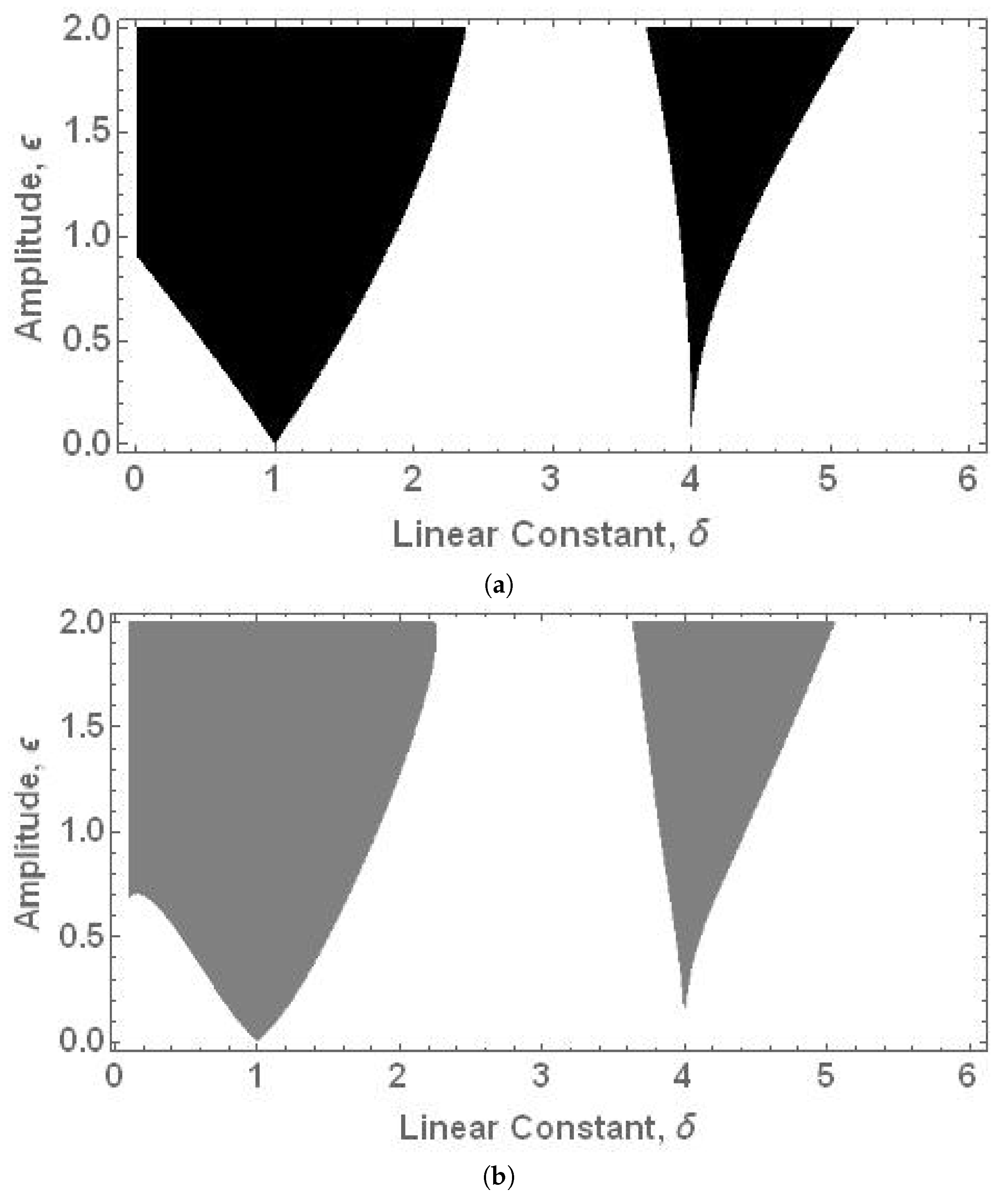
As explained earlier, the SSF dynamical model was reduced of the form Equation (49), where $\delta$ is linear constant term and $2ϵ$ is the amplitude of the parametric excitation. When $\eta =2$, the principal period of the system is $T=\pi$ secs. The standard Mathieu Equation (49) was numerically integrated for different sets of initial conditions (${\theta }_0=1.0,{\dot{\theta }}_0=0.0$ and ${\theta }_0=0.0,{\dot{\theta }}_0=1.0$) and the system states were evaluated at the principal period (T). The values of system states were concatenated such that the Floquet theory was applied to identify the stability bounds numerically, as detailed in [59]. The condition of both the Floquet multipliers being on or inside the unit circle was used as the criterion for identifying the stability bounds. The standard template of the system parameter variation in the ($\delta -ϵ$) plane was adapted to generate the plots shown in Figure 5a.

Meanwhile, as detailed in Section 2.2, the periodic term in Equation (49) is augmented, resulting in the updated equation as

$$\frac{d}{d\tau }\left\{\begin{array}{c}\theta \\ \dot{\theta }\\ p\\ \dot{q}\end{array}\right\}=\left[\begin{array}{cccc}0& 1& 0& 0\\ -\delta & 0& 0& 0\\ 0& 0& 0& 1\\ 0& 0& -{\eta }^2& 0\end{array}\right]\left\{\begin{array}{c}\theta \\ \dot{\theta }\\ p\\ \dot{q}\end{array}\right\}+\left\{\begin{array}{c}0\\ 2ϵ\theta p\\ 0\\ 0\end{array}\right\}$$

(51)

where $p=cos\left(\eta \tau \right);q=-\eta sin\left(\eta \tau \right)$. The Equation (51) is in the form similar to Equation (11) and undergoes modal transformation and near-identity transformation to apply the Normal Forms technique, as explained in Section 2.3. The Floquet multipliers from the reduced Normal Forms solution were computed as per Equation (28) and utilized to generate the stability plot indicated in Figure 5b.

In Figure 5, the shaded area indicates the unstable region and white area indicates the stable region for the standard Mathieu equation. It is observed that the plot generated using the Normal Forms solution (Figure 5b) replicates the one from the Floquet Theory application on numerically integrated results (Figure 5a) quite well. Both these plots agree with the results obtained in [59]. This validates the application of the Normal Forms solution towards stability analysis of time periodic systems.

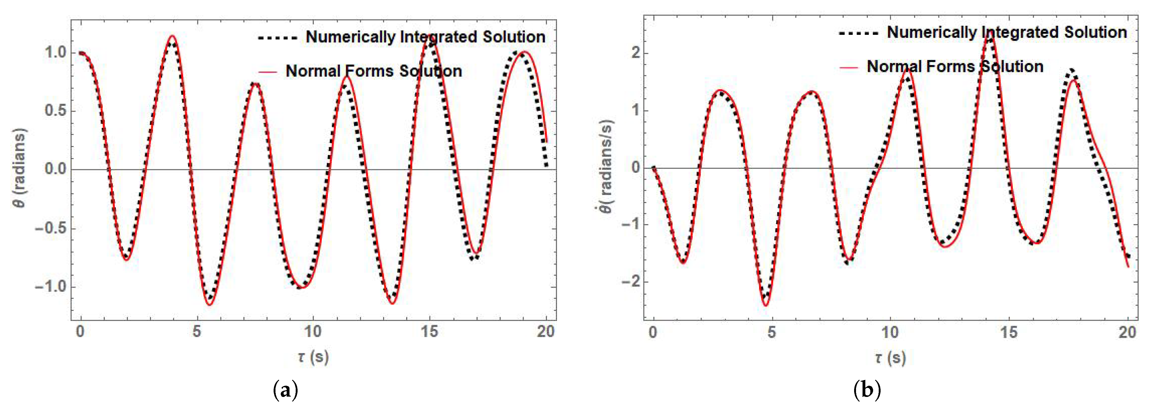
From both the sub-figures in Figure 5, the system parameters $\delta =3.0$ and $ϵ=1.0$ corresponds to a stable point. The STM of the reduced Normal forms solution is back transformed to obtain $\widehat{\mathsf{\Phi }}\left(t\right)$ matrix. This matrix is then multiplied with the initial conditions of the system states in Equation (49) to determine the system state evolution. Simultaneously, Equation (49) was numerically integrated with the same value of system parameters and initial conditions (${\theta }_0=1,{\dot{\theta }}_0=0$). The comparison of the variations of the system states are plotted in Figure 6.

As mentioned in Figure 6, the red solid line indicates the temporal variation based on the STM, $\widehat{\mathsf{\Phi }}\left(t\right)$, determined from the Normal Forms technique and the black dashed line represents the numerically integrated solution of Equation (49). In both plots, the system is observed to follow a stable bounded periodic behavior and does not deviate away from the initial conditions.

5.2. SSF with Significant Linear Damping ($\overline{B}=1.0$)

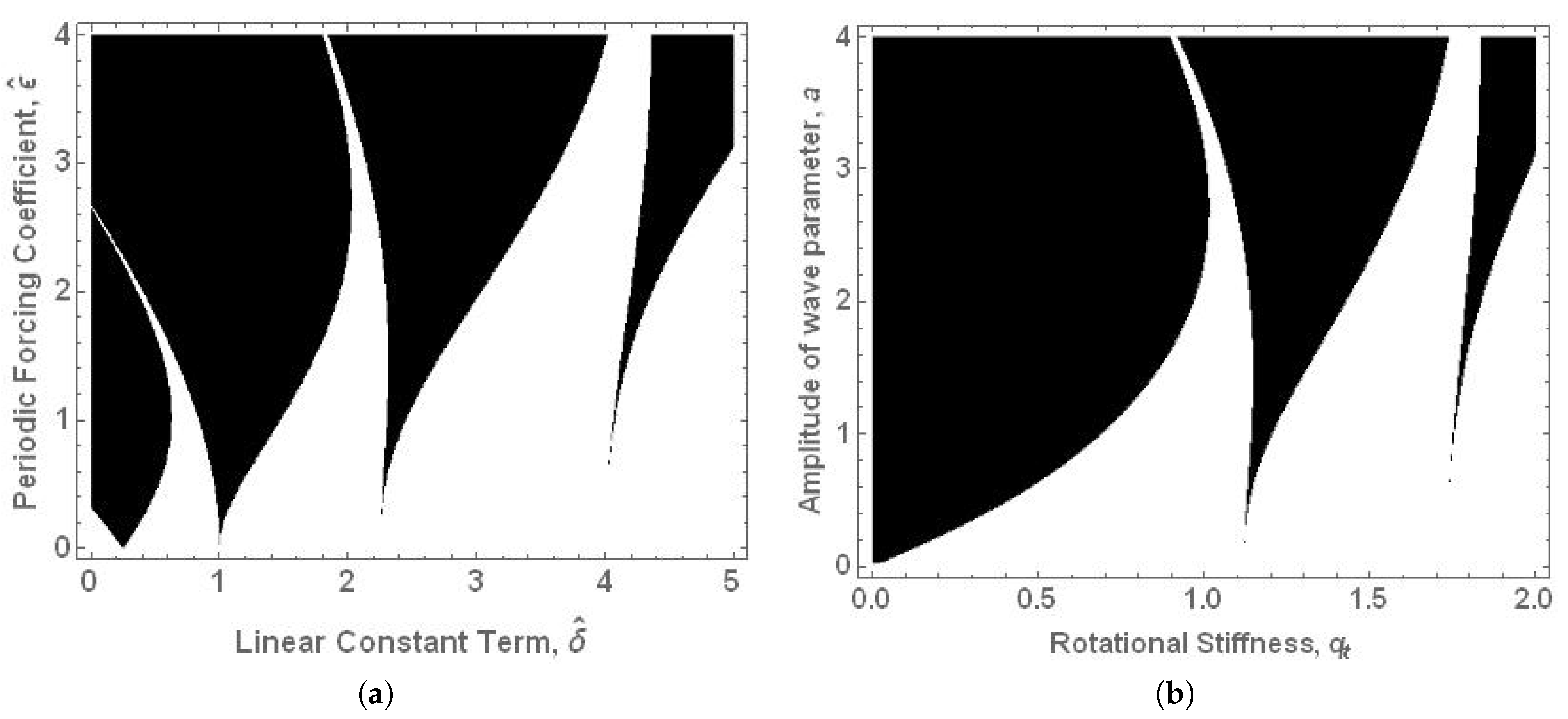
For the case of SSF model with significant linear damping, the SSF dynamical behavior is represented by Equation (50). Since this system is also considered to be a Mathieu equation, the stability plots are initially generated in the standard template of ($\widehat{\delta }-\widehat{ϵ}$) plane. Though the linear constant term variation ($\widehat{\delta }$) is only attributed to the rolls stiffness ($q_t$), the coefficient of periodic forcing term ($\widehat{ϵ}$) comprises of many variables corresponding to the wave motions. By considering the linear stiffness parameter, $q=1$ and the frequency parameter, $\eta =1$(thereby setting the principal time period for analysis to be $T=2\pi$ seconds), the variation in $\widehat{ϵ}$ is solely attributed towards the variation in amplitude of wave term (a). Hence, similar stability plots can be generated in the ($a-q_t$) plane for the equivalent range of parameters from ($\widehat{\delta }-\widehat{ϵ}$) plane. For the given set of system parameters, the system equation (Equation (50)) is numerically integrated and both the stability plots are generated based on the Floquet multiplier condition, as displayed in Figure 7a,b.

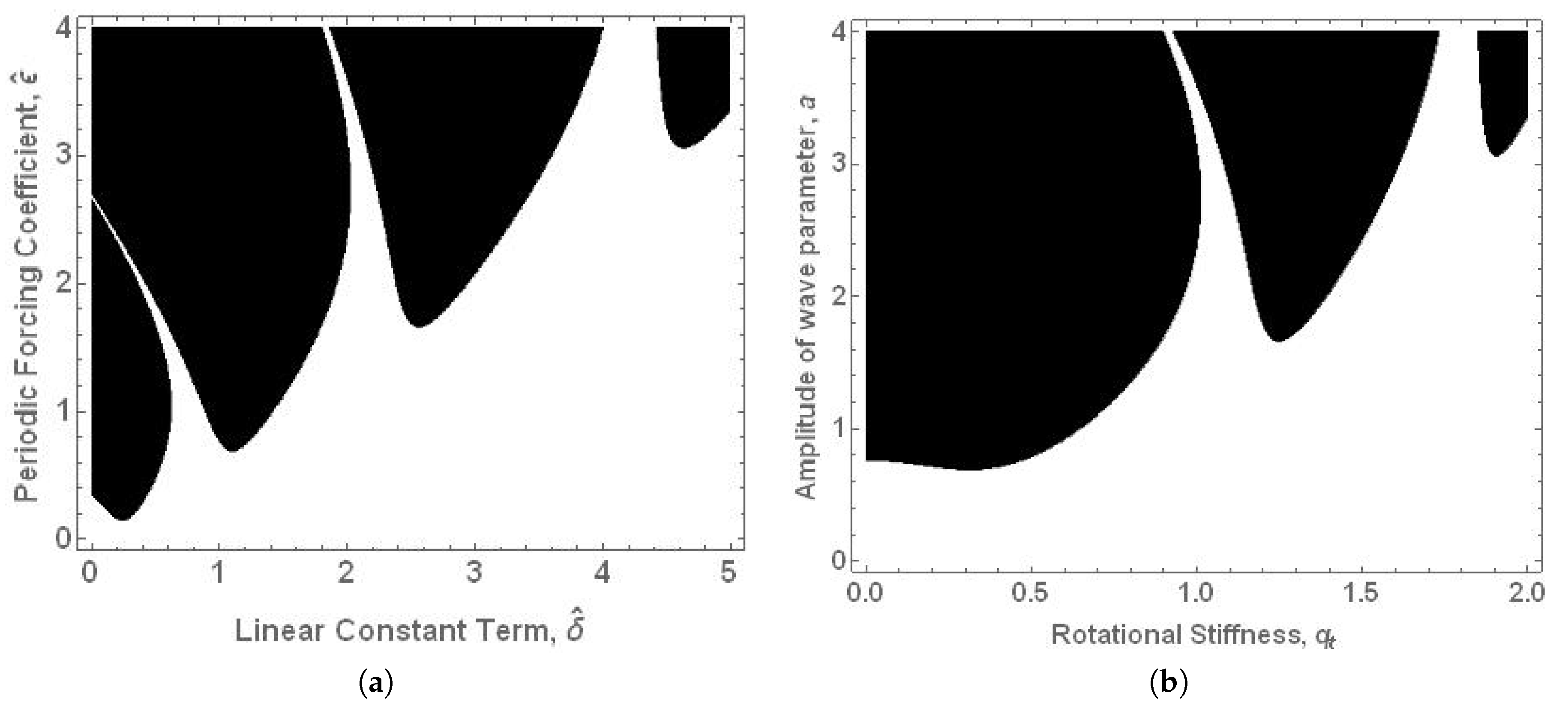
Later, for the same set of system parameters, an external rotational damper of ($\overline{C}=0.2$) was added and investigated for the stability characteristics. Again the stability plots were generated based on the Floquet multiplier condition, as indicated in Figure 8a,b.

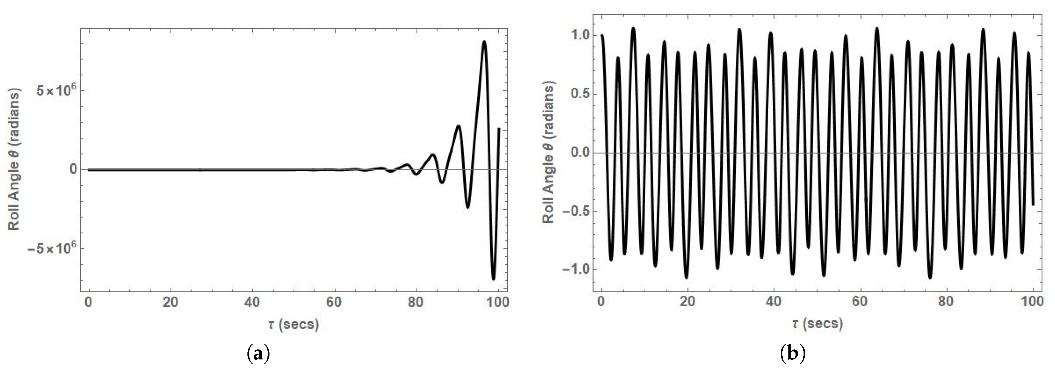
In both Figure 7 and Figure 8, the white area indicates the stable region of operation and the black/shaded region represents the unstable region of operation for the SSF platform. Though the frequency of sea waves vary, similar trend are observed for the stability plots at a particular wave frequency. In both Figure 7b and Figure 8b, the point corresponding to system parameters ($q_t=0.5,a=1.0$), the system is observed to be unstable. As the torsional/rotational stiffness is updated to $q_t=1.50$, keeping the amplitude of wave parameter as $a=1.0$, the SSF system is observed to be in the stable zone. To verify the same, the roll angle variations in Equation (48) is numerically integrated with the initial conditions (${\theta }_0=1.0,{\dot{\theta }}_0=0.0$). Initially the roll angle variations for the SSF system with significant linear damping and no rotational damper are evaluated and plotted in Figure 9.

Similarly, the roll angle variations for the SSF system with significant linear damping and an additional rotational damper ($\overline{C}=0.20$) is evaluated and plotted in Figure 10.

6. Discussion

The expression for the suction stabilization effect(Equation (38)), indicates that torsional spring stiffness is directly proportional to the area of the base of the internal chamber. This intuitively provides an insight that higher the base area, higher will be the suction stabilization effect. It can be also inferred that for higher restoring moment, design the SSF with larger base area at the water level. This can also be achieved by attaching multiple small units of SSF floats. As mentioned earlier, in the dynamical modelling, it was observed that the roll motion of the reduced order of SSF model characterizes the stability features of the heave-roll coupled model. This also provides an insight towards the energy transfer within the SSF model.

For the heave motions attained with negligible linear damping, the roll motion of SSF dynamical model follows a standard Mathieu equation. The stability plot in Figure 5, exhibits that the stable region (in white) increases considerably as the linear constant ($\delta$) increases. The $\delta$ term replaced the $(1+q_t^2)$ term in Equation (48), which in turn was directly proportional to the suction stabilization effect. Hence it could also be concluded that in the reduced SSF model, the increase in torsional stiffness term ($q_t$) increases the stable bounds of the system. The temporal variations of system states from the back-transformed Normal Forms solution, follows the numerical integration results closely, as shown in Figure 6. This validates the direct application of Normal Forms technique with the aid of state augmentation.

For the heave motions attained with significant linear damping, the roll motion of the SSF dynamical model follows a modified Mathieu equation (Equation (50)). Though the parameters used for the stability plots are similar in this case, the effect of linear damping is evident in Figure 7a and Figure 8a. The stability bounds have been lifted from the x-axis. However, the rotational stiffness parameter ($q_t$) is still observed to contribute towards the stability. As the value of the rotational stiffness parameter ($q_t$) increases, the stability bounds are observed to be more, even when the amplitude of wave parameter (a) is high. Moreover, in Figure 8a,b, the additional rotational damper ($\overline{C}$) is observed to smoothing the transition curves such that the stable bounds are further increased. This trend of the stability plots is observed to remain the same even with higher values of wave frequency. The additional rotational damper can be attributed to one or a combination of the add-on techniques in the float design or an active controller. To validate the stability characteristics, an unstable and stable point is selected from both Figure 7b and Figure 8b and the temporal variations are plotted with the corresponding system parameters.

Figure 9a corresponds to the roll motion of the SSF model with significant linear damping and no rotational damping when $q_t=0.5,a=1.0$. In Figure 7b, this corresponds to the unstable region and it is observed that roll motion amplifies unbounded and could result in the float getting capsized. Whereas Figure 9b corresponds to the roll motion of the SSF model with significant linear damping and no rotational damping when $q_t=1.5,a=1.0$. In Figure 7b, this corresponds to the stable region and it is observed to exhibit a bounded roll motion over time. This validates the stability plots in Figure 7.

In case of the SSF model with significant linear damping and additional rotational damper ($\overline{C}=0.2$), the point ($q_t=0.5,a=1.0$) in Figure 8b again corresponds to the unstable region. Though it is also evident from Figure 10a that the roll motions grow unbounded, the range of motion has reduced drastically for the same time period. This indicates that the additional damper has some effect in reducing the amplitude of the roll motion, but it is still not capable of stabilizing the float. However, when the rotational stiffness parameter value ($q_t$) is increased to $q_t=1.5$, the system is observed to be stable, as per Figure 8b. Additionally, the roll motions corresponding to $q_t=1.5,a=1.0$, in Figure 10b almost dampen out by 50 s. Hence, the stability plots in Figure 8 are validated and it can also be concluded that the higher value of the rotational stiffness ($q_t$) aids in stabilizing the SSF platform, which is associated to the suction stabilization effect. It can be also inferred that the additional rotational damper in conjunction with the suction stabilization is capable of making the float attain a stable fixed point and no just a stable periodic motion. As discussed, a stable fixed point is more desirable for offshore structures in most of the applications.

7. Conclusions

In this work, the authors provide a brief explanation on various mathematical concepts utilized towards dynamical analysis applicable for analyzing a SSF platform. Later, the effect of suction stabilization was mathematically derived for the case of a symmetrically shaped float/platform. Subsequently, the authors compared the dynamical behavior of SSF to ship motions and derived the equations of motion for SSF using a heave-roll model. A model order reduction was performed on the resulting equations of motion to facilitate the dynamical analysis. It was demonstrated that all the major dynamical characteristics (including that of heave motions) could be represented in the reduced order roll motions. The reduced order roll motions were observed to be comparable to a parametrically excited Mathieu equation. The authors employ Floquet theory and Normal Forms technique to analytically assess the stability bounds of a SSF platform exposed to periodic sea waves. The temporal variations of the model were verified numerically to validate the dynamical characteristics of a SSF platform. The suction stabilization effect is proven to be aiding in the stability of offshore floats in this paper and further verification with experimental results will be presented in future work.

In this work, the sea waves were considered to be periodic in nature. However, in reality they could be expressed as quasi-periodic system with incommensurate frequencies. The direct approach of Normal Forms technique could be extended towards quasi-periodic system as well. The dynamical behavior of SSF platform with quasi-periodic base excitation will be analyzed and published in future work.

8. Patents

The design for suction stabilized float has been patented (US20120090525A1) [60].

References

- Castro-Santos, L.; Bento, A.R.; Silva, D.; Salvação, N.; Guedes Soares, C. Economic Feasibility of Floating Offshore Wind Farms in the North of Spain. J. Mar. Sci. Eng. 2020, 8, 58. [Google Scholar] [CrossRef] [Green Version]
- Wayman, E.N.; Sclavounos, P.; Butterfield, S.; Jonkman, J.; Musial, W. Coupled Dynamic Modeling of Floating Wind Turbine Systems; Technical Report; National Renewable Energy Lab. (NREL): Golden, CO, USA, 2006. [Google Scholar]
- Butterfield, S.; Musial, W.; Jonkman, J.; Sclavounos, P. Engineering Challenges for Floating Offshore wind Turbines; Technical Report; National Renewable Energy Lab. (NREL): Golden, CO, USA, 2007. [Google Scholar]
- James, R.; Ros, M.C. Floating Offshore Wind: Market and Technology Review; Technical Report; The Carbon Trust: London, UK, 2015. [Google Scholar]
- Karimi, M.; Hall, M.; Buckham, B.; Crawford, C. A multi-objective design optimization approach for floating offshore wind turbine support structures. J. Ocean Eng. Mar. Energy 2017, 3, 69–87. [Google Scholar] [CrossRef]
- Yang, W.H.; Yang, R.Y.; Chang, T.C. Experimental and numerical study of the stability of barge-type floating offshore wind turbine platform. In EGU General Assembly Conference Abstracts; EGU: Munich, Germany, 2020; p. 10179. [Google Scholar]
- Odijie, A.C.; Wang, F.; Ye, J. A review of floating semisubmersible hull systems: Column stabilized unit. Ocean Eng. 2017, 144, 191–202. [Google Scholar] [CrossRef] [Green Version]
- Thiagarajan, K.; Dagher, H. A review of floating platform concepts for offshore wind energy generation. J. Offshore Mech. Arct. Eng. 2014, 136, 020903. [Google Scholar] [CrossRef]
- Modi, P.; Seth, S. Hydraulics and Fluid Mechanics (Including Hydraulic Machines) (in Metric Units); Standard Book House: New Delhi, India 1980. [Google Scholar]
- Biran, A.; Pulido, R.L. Ship Hydrostatics and Stability; Butterworth-Heinemann: Oxford, UK, 2013. [Google Scholar]
- Corvaro, S.; Crivellini, A.; Marini, F.; Cimarelli, A.; Capitanelli, L.; Mancinelli, A. Experimental and Numerical Analysis of the Hydrodynamics around a Vertical Cylinder in Waves. J. Mar. Sci. Eng. 2019, 7, 453. [Google Scholar] [CrossRef] [Green Version]
- Amaechi, C.V.; Wang, F.; Hou, X.; Ye, J. Strength of submarine hoses in Chinese-lantern configuration from hydrodynamic loads on CALM buoy. Ocean Eng. 2019, 171, 429–442. [Google Scholar] [CrossRef] [Green Version]
- Li, Y.; Le, C.; Ding, H.; Zhang, P.; Zhang, J. Dynamic response for a submerged floating offshore wind turbine with different mooring configurations. J. Mar. Sci. Eng. 2019, 7, 115. [Google Scholar] [CrossRef] [Green Version]
- Konovessis, D.; Chua, K.H.; Vassalos, D. Stability of floating offshore structures. Ships Offshore Struct. 2014, 9, 125–133. [Google Scholar] [CrossRef]
- Zhang, H.; Xu, D.; Xia, S.; Wu, Y. A new concept for the stability design of floating airport with multiple modules. Procedia IUTAM 2017, 22, 221–228. [Google Scholar] [CrossRef]
- Utsunomiya, T.; Matsukuma, H.; Minoura, S.; Ko, K.; Hamamura, H.; Kobayashi, O.; Sato, I.; Nomoto, Y.; Yasui, K. At sea experiment of a hybrid spar for floating offshore wind turbine using 1/10-scale model. J. Offshore Mech. Arct. Eng. 2013, 135. [Google Scholar] [CrossRef]
- Wang, H.; Somayajula, A.; Falzarano, J.; Xie, Z. Development of a blended time-domain program for predicting the motions of a wave energy structure. J. Mar. Sci. Eng. 2020, 8, 1. [Google Scholar] [CrossRef] [Green Version]
- Davidson, J.; Costello, R. Efficient Nonlinear Hydrodynamic Models for Wave Energy Converter Design—A Scoping Study. J. Mar. Sci. Eng. 2020, 8, 35. [Google Scholar] [CrossRef] [Green Version]
- Giorgi, G.; Davidson, J.; Habib, G.; Bracco, G.; Mattiazzo, G.; Kalmár-Nagy, T. Nonlinear Dynamic and Kinematic Model of a Spar-Buoy: Parametric Resonance and Yaw Numerical Instability. J. Mar. Sci. Eng. 2020, 8, 504. [Google Scholar] [CrossRef]
- Sultania, A.; Manuel, L. Extreme loads on a spar buoy-supported floating offshore wind turbine. In Proceedings of the 51st AIAA/ASME/ASCE/AHS/ASC Structures, Structural Dynamics, and 12th Materials Conference 18th AIAA/ASME/AHS Adaptive Structures Conference, Orlando, FL, USA, 12–15 April 2010; p. 2738. [Google Scholar]
- Paulling, J.R. On unstable ship motions resulting from nonlinear coupling. J. Ship Res. 1959, 3, 36–46. [Google Scholar]
- Bass, D. On the response of biased ships in large amplitude waves. Int. Shipbuild. Prog. 1983, 30, 2–9. [Google Scholar] [CrossRef]
- Oh, I.G.; Nayfeh, A.H.; Mook, D.T. A theoretical and experimental investigation of indirectly excited roll motion in ships. Philos. Trans. R. Soc. A Math. Phys. Eng. Sci. 2000, 358, 1853–1881. [Google Scholar] [CrossRef]
- Nayfeh, A.H.; Mook, D.T.; Marshall, L.R. Nonlinear coupling of pitch and roll modes in ship motions. J. Hydronautics 1973, 7, 145–152. [Google Scholar] [CrossRef]
- Oh, I.; Nayfeh, A.; Mook, D. Theoretical and experimental study of the nonlinearity coupled heave, pitch, and roll motions of a ship in longitudinal waves. In Proceedings of the 19th Symposium on Naval Hydrodynamics, Seoul, Korea, 23–28 August 1992; National Academy Press: Washington, DC, USA, 1994. [Google Scholar]
- Iakubovich, V.A.; Starzhinskiĭ, V.M. Linear Differential Equations with Periodic Coefficients; Wiley: New York, NY, USA, 1975; Volume 2. [Google Scholar]
- Nayfeh, A.H. Introduction to Perturbation Techniques; Wiley-VCH: Weinheim, Germany, 2011. [Google Scholar]
- Sanders, J.A.; Verhulst, F.; Murdock, J.A. Averaging Methods in Nonlinear Dynamical Systems; Springer: New York, NY, USA, 2007; Volume 59. [Google Scholar]
- Sinha, S.C.; Pandiyan, R.; Bibb, J. Liapunov-Floquet transformation: Computation and applications to periodic systems. J. Vib. Acoust. 1996, 118, 209–219. [Google Scholar] [CrossRef]
- Sharma, A.; Sinha, S.C. An approximate analysis of quasi-periodic systems via Floquét theory. J. Comput. Nonlinear Dyn. 2018, 13, 021008. [Google Scholar] [CrossRef]
- Chen, C.W.; Shen, C.W.; Chen, C.Y.; Cheng, M.J. Stability analysis of an oceanic structure using the Lyapunov method. Eng. Comput. 2010, 27, 186–204. [Google Scholar] [CrossRef]
- Sinha, S.; Wu, D.H.; Juneja, V.; Joseph, P. Analysis of dynamic systems with periodically varying parameters via Chebyshev polynomials. J. Vib. Acoust. 1993, 115, 96–102. [Google Scholar] [CrossRef]
- Sinha, S.; Juneja, V. An approximate analytical solution for systems with periodic coefficients via symbolic computation. In Proceedings of the 32nd Structures, Structural Dynamics, and Materials Conference, Baltimore, MD, USA, 8–10 April 1991; p. 1020. [Google Scholar]
- Sinha, S.; Gourdon, E.; Zhang, Y. Control of time-periodic systems via symbolic computation with application to chaos control. Commun. Nonlinear Sci. Numer. Simul. 2005, 10, 835–854. [Google Scholar] [CrossRef]
- Poincaré, H. Les méthodes Nouvelles de la Mécanique Céleste; Gauthier-Villars et Fils: Paris, France, 1899; Volume 3. [Google Scholar]
- Birkhoff, G.D. Dynamical Systems; American Mathematical Soc.: Providence, RI, USA, 1927; Volume 9. [Google Scholar]
- Moser, J.; Saari, D. Stable and random motions in dynamical systems. Phys. Today 1975, 28, 47. [Google Scholar] [CrossRef]
- Arnold, V. Mathematical Methods of Classical Mechanics. Ann. Arbor 1978, 1001, 48109. [Google Scholar]
- Chua, L.O.; Kokubu, H. Normal forms for nonlinear vector fields. I. Theory and algorithm. IEEE Trans. Circuits Syst. 1988, 35, 863–880. [Google Scholar] [CrossRef]
- Nayfeh, A.H. The Method of Normal Forms; Wiley-VCH: Weinheim, Germany, 2011. [Google Scholar]
- Murdock, J. Normal Forms and Unfoldings for Local Dynamical Systems; Springer: New York, NY, USA, 2006. [Google Scholar]
- Smith, H.L. Normal forms for periodic systems. J. Math. Anal. Appl. 1986, 113, 578–600. [Google Scholar] [CrossRef] [Green Version]
- Sinha, S.; Butcher, E.; Dávid, A. Construction of dynamically equivalent time-invariant forms for time-periodic systems. Nonlinear Dyn. 1998, 16, 203–221. [Google Scholar] [CrossRef]
- Gabale, A.P.; Sinha, S. A direct analysis of nonlinear systems with external periodic excitations via normal forms. Nonlinear Dyn. 2009, 55, 79–93. [Google Scholar] [CrossRef]
- Jezequel, L.; Lamarque, C.H. Analysis of non-linear dynamical systems by the normal form theory. J. Sound Vib. 1991, 149, 429–459. [Google Scholar] [CrossRef]
- Waswa, P.M.; Redkar, S. A direct approach for simplifying nonlinear systems with external periodic excitation using normal forms. Nonlinear Dyn. 2020, 99, 1065–1088. [Google Scholar] [CrossRef]
- Waswa, P.M.; Redkar, S.; Subramanian, S.C. A plain approach for center manifold reduction of nonlinear systems with external periodic excitations. J. Vib. Control 2019, 26, 929–940. [Google Scholar] [CrossRef]
- Susheelkumar, C.; Redkar, S.; Sugar, T. Parametric resonance and energy transfer in suction stabilized floating platforms: A brief survey. Int. J. Dyn. Control 2017, 5, 931–945. [Google Scholar] [CrossRef]
- Sinha, S.; Pandiyan, R. Analysis of quasilinear dynamical systems with periodic coefficients via Liapunov-Floquet transformation. Int. J. Non-Linear Mech. 1994, 29, 687–702. [Google Scholar] [CrossRef]
- Faltinsen, O.M. Hydrodynamics of High-Speed Marine Vehicles; Cambridge University Press: New York, NY, USA, 2005. [Google Scholar]
- Harris, J.W.; Stöcker, H. Handbook of Mathematics and Computational Science; Springer: New York, NY, USA, 1998. [Google Scholar]
- Nabergoj, R.; Tondl, A.; Virag, Z. Autoparametric resonance in an externally excited system. Chaos Solitons Fractals 1994, 4, 263–273. [Google Scholar] [CrossRef]
- Tondl, A.; Tondl, A.; Ruijgrok, M.; Ruijgrok, T.; Nabergoj, R.; Verhulst, F. Autoparametric Resonance in Mechanical Systems; Cambridge University Press: New York, NY, USA, 2000. [Google Scholar]
- Cheung, K.; Phadke, A.; Smith, D.; Lee, S.; Seidl, L. Hydrodynamic response of a pneumatic floating platform. Ocean Eng. 2000, 27, 1407–1440. [Google Scholar] [CrossRef]
- Vidic-Perunovic, J. Influence of the GZ calculation method on parametric roll prediction. Ocean Eng. 2011, 38, 295–303. [Google Scholar] [CrossRef]
- Ibrahim, R.; Grace, I. Modeling of ship roll dynamics and its coupling with heave and pitch. Math. Probl. Eng. 2010, 2010, 934714. [Google Scholar] [CrossRef] [Green Version]
- Ellermann, K.; Kreuzer, E.; Markiewicz, M. Nonlinear dynamics of floating cranes. Nonlinear Dyn. 2002, 27, 107–183. [Google Scholar] [CrossRef]
- Aburn, M. Critical Fluctuations and Coupling of Stochastic Neural Mass Models. Ph.D. Thesis, The University of Queensland, St. Lucia, Australia, 2016. [Google Scholar]
- Kovacic, I.; Rand, R.; Mohamed Sah, S. Mathieu’s equation and its generalizations: Overview of stability charts and their features. Appl. Mech. Rev. 2018, 70, 020802. [Google Scholar] [CrossRef] [Green Version]
- Montgomery, J. Suction Stabilized Floats. U.S. Patent 10,239,590, 26 March 2019. [Google Scholar]
Figure 1.
Righting arm.
Figure 2.
Suction Stabilized Floating (SSF) platform (a) Front View, (b) Top View.
Figure 3.
SSF Platform heeled by an angle .
Figure 4.
Heave-roll model for SSF.
Figure 5.
Comparison of Stability plots for standard Mathieu equation, where the shaded area corresponds to unstable bounds and white area corresponds to stable bounds (a) Generated using numerical integration and Floquet theory, (b) Generated from the Normal Forms Solutions.
Figure 6.
Comparison of temporal variations of the reduced SSF system states (a) Roll angle variation with respect to time, (b) Roll angular rate variation with respect to time.
Figure 7.
Stability plot for SSF with significant linear damping and without rotational damping (a) in plane, (b) in plane.
Figure 8.
Stability plot for SSF with significant linear damping and with rotational damping (a) in plane, (b) in plane.
Figure 9.
Comparison of roll angle variations of the SSF system with significant linear damping and no rotational damper (a) when , (b) when .
Figure 10.
Comparison of roll angle variations of the SSF system with significant linear damping and an additional rotational damper () (a) when , (b) when .
© 2020 by the authors. Licensee MDPI, Basel, Switzerland. This article is an open access article distributed under the terms and conditions of the Creative Commons Attribution (CC BY) license (http://creativecommons.org/licenses/by/4.0/).
Share and Cite
MDPI and ACS Style
C. Subramanian, S.; Dye, M.; Redkar, S. Dynamic Analysis of Suction Stabilized Floating Platforms. J. Mar. Sci. Eng. 2020, 8, 587. https://doi.org/10.3390/jmse8080587
AMA Style
C. Subramanian S, Dye M, Redkar S. Dynamic Analysis of Suction Stabilized Floating Platforms. Journal of Marine Science and Engineering. 2020; 8(8):587. https://doi.org/10.3390/jmse8080587
Chicago/Turabian StyleC. Subramanian, Susheelkumar, Michaela Dye, and Sangram Redkar. 2020. "Dynamic Analysis of Suction Stabilized Floating Platforms" Journal of Marine Science and Engineering 8, no. 8: 587. https://doi.org/10.3390/jmse8080587
Note that from the first issue of 2016, this journal uses article numbers instead of page numbers. See further details here.