A Coupled Artificial Compressibility Method for Free Surface Flows


School of Naval Architecture & Marine Engineering, National Technical University of Athens, 15780 Zografos, Greece
*
Author to whom correspondence should be addressed.
J. Mar. Sci. Eng. 2020, 8(8), 590; https://doi.org/10.3390/jmse8080590
Submission received: 14 July 2020
/
Revised: 31 July 2020
/
Accepted: 4 August 2020
/
Published: 6 August 2020
(This article belongs to the Special Issue Wave Phenomena in Ship and Marine Hydrodynamics)
Abstract
:Modeling free surface flows in a CFD context typically requires an incompressible approach along with a formulation to account for the air–water interface. Commonly, pressure-correction algorithms combined with the Volume of Fluid (VOF) method are used to describe these kinds of flows. Pressure-correction algorithms are segregated solvers, which means equations are solved in sequence until convergence is accomplished. On the contrary, the artificial compressibility (AC) method solves a single coupled system of equations. Solving at each timestep a single system of equations obviates the need for segregated algorithms, since all equations converge simultaneously. The goal of the present work is to combine the AC method with VOF formulation and prove its ability to account for unsteady flows of immiscible fluids. The presented system of equations has a hyperbolic nature in pseudo-time, thus the arsenal of the hyperbolic discretization process can be exploited. To this end, a thorough investigation of unsteady flows is presented to demonstrate the ability of the method to accurately describe unsteady flows. Problems of wave propagation on constant and variable bathymetry are considered, as well as a fluid structure interaction problem, where viscous effects have a significant impact on the motion of the structure. In all cases the results obtained are compared with theoretical or experimental data. The straightforward implementation of the method, as well as its accurate predictions, shows that AC method can be regarded as a suitable choice to account for free surface flows.
1. Introduction
Free surface flows pose significant challenges when it comes to numerical modeling. Accurate modeling of the free surface is crucial in many engineering applications ranging from ship hydrodynamics to floating platforms. Additionally, for the proper hydrodynamic and structural design of marine vessels and offshore structures, it is mandatory to take into account wave–structure interaction. To that end, several numerical methods have been developed of varying fidelity. Boundary element methods (BEM) have been widely used in the literature to model non-linear free surface waves [1]. They can provide accurate results at a small computational cost [2] and can be easily coupled with other numerical frameworks (e.g., hydro-aero-elastic solvers [3]). More sophisticated models have been also developed [4] reducing the problem size and consequently the computational cost. However, potential methods do not account for viscosity and the usual remedy is to apply viscous correction on the results [5].
When viscous effects become significant, the usual approach is to employ a computational fluid dynamic (CFD) framework. Space is discretized using structured/unstructured grids and the Reynolds Averaged Navies-Stokes (RANS) equations are solved on the underlying mesh. Two main categories of methodologies have been developed to account for free surface flows. On the one hand, the surface tracking methods [6,7] describe the free surface as a moving boundary, with the appropriate boundary conditions, and the solution process involves only the liquid phase. Deforming grids are used to track the motion of the free surface boundary. On the other hand, the other broad category for free surface flows are the surface capturing methods. In this case, the free surface is identified as density discontinuity and both liquid and air phase are resolved. In respect to the free surface capturing approach, there are several options, namely the Volume of Fluid method (VOF) [8], the Level Set method [9] and the Marker-and-Cell method (MAC) [10]. In this approach an additional equation is added to the system of equations expressing the general fluid properties. Finally, a third category has been introduced, where a hybrid formulation of a potential approach combined with the RANS numerical framework is used [11]. In all cases, the flow is treated as incompressible even though recently there are several works that consider compressibility effects in the air phase [12,13].
The assumption of incompressible flow poses further complexity in the numerical procedure. The complication arises from the fact that there is no equation for the time evolution of pressure that satisfies the kinematic constraint of the continuity equation. A straightforward discretization of the incompressible equations will lead to spurious oscillations (checkerboard problem). One of the first attempts to tackle the decoupling of the momentum and mass equation is the Staggered Grid approach [10]. In this framework, the unknown variables are computed in grid points which are staggered with respect to each other. It is the most straightforward solution to the checkerboard problem, and it is the method of choice for orthogonal grids. Another approach is the fractional step methods [14], where an operator splitting is performed and the convective, diffusive and pressure terms are accounted in different steps. The most well-known and broadly used algorithms accounting for incompressible flows are the projection methods and its variants pressure-correction algorithms (e.g., PISO [15], SIMPLE [16], etc.). These methods attempt the inter-equation coupling by perturbating the mass equation with pressure terms. These algorithms are segregated, meaning that equations are solved in sequence. In the two-phase flows context, projection methods are by far the most employed approach to the incompressible equations [17,18], while fractional step methods are recently also employed in the literature [19].
Contrary to pressure-correction methods the artificial compressibility (AC) method [20,21,22] solves the incompressible equation in a non-segregated manner. The coupling is performed by adding a pressure derivative to the continuity equation that vanishes when convergence is accomplished. Employing the AC method gives rise to a hyperbolic (for the convective terms) coupled system of equations in pseudo-time. Upon convergence the original set of equation is restored. Consequently, the numerical techniques developed for hyperbolic systems (e.g., approximate Riemann solvers) can be used. Additionally, it removes the need for segregated algorithms since a single system of equations is formed. On the other hand, the fully coupled system of equations is formed at the expense of an arbitrary parameter ().
For one-phase flows the AC method is widely used; however, in the multiphase flows context the literature is rather limited. In [23] they successfully formulated an AC method for free surface flows in close containers. Kunz et al. [24] applied a preconditioned AC approach for cavitating flows while [25] handled the steady state wave problem. Nevertheless, to the authors’ knowledge, employing an AC formulation to unsteady water wave problems is not explored in the literature.
This paper, based on the work of Kunz et al. [24], proposes an artificial compressibility approach to simulate free surface flows. We present an AC framework coupled with the VOF approach for unsteady water flows. A series of numerical experiments are conducted to prove the validity of the method. Furthermore, we investigate the effect of the AC parameter and guidelines for its values are given. Finally, an implicit method to generate and absorb free surface waves is presented.
The present methodology was implemented as an extension to the compressible solver MaPFlow [26,27]. MaPFlow is developed at NTUA and it is an unstructured cell-centered finite volume solver, that solves the unsteady Reynolds Averaged Navier–Stokes equations. The solver is parallelized by using the MPI protocol, while the grid partitioning is performed by the Metis library [28].
The paper is structured as follows. Section 2 and Section 3 present Mathematical and Numerical modeling, while Section 4 includes the analysis of various method parameters. In addition, MaPFlow’s predictions are validated against available experimental data. The case of wave propagation over a variable bathymetry is considered and compared to measurements available from [29]. Also, a fluid–structure interaction problem of a moonpool-type floater is considered and predictions are compared with available experimental data from [30]. Finally, in Section 5 the basic conclusions are outlined.
2. Governing Equations
The VOF method uses an indicator function to describe the presence of the liquid or the gas phase. Specifically, let be the water density and the density of the air, then the volume fraction is defined as . The volume fraction is equal to 0 in regions occupied by the air phase, equals to 1 when only the water phase is present and takes values between 0 and 1 near the free surface. The interface of the fluids is located in regions of rapid change of the gradient of the indicator function. The properties of the mixture fluid, density () and dynamic viscosity (), are described by the blending Function (1).
The free surface, as presented in Equation (2), is considered to be a material surface.
where is the three-dimensional velocity vector, is the divergence operator and t denotes the real time variable.
The artificial compressibility method attempts to overcome the decoupling of the mass and momentum equations by augmenting the mass equation with a pseudo-time derivative of pressure (p), as it is shown in Equation (3). The influence of pseudo-time derivative is regulated by the artificial compressibility factor .
denotes the pseudo-time variable.
The pseudo-time derivative corresponds to the iterative numerical procedure until convergence. In order to obtain the original equation, the pseudo-time derivative of the convergent solution should be equals to zero.
The essence of the AC method is that it assumes a relation between pressure and density during convergence (Equation (4)). This relation is similar to compressible definition of sound speed. However, in this case the parameter is a numerical parameter that regulates convergence.
Equation (4) gives rise to a pseudo-sound speed definition. In case of one-dimensional, one-phase flows, the artificial speed of sound is given by Equation (5). The sound speed is regulated through the artificial parameter . In Appendix A it is shown that the pseudo-sound speed regulates the convergence in a similar way that the sound speed effects the compressible equations.
Regarding the simulation of two-phase flows, the momentum equations written in a conservative form and expressed in terms of the mixture quantities are presented in Equation (6), along with the VOF equation expressed also, in conservative form.
In previous equations, is the stress tensor and the vector includes source terms and body forces.
The Equations (3) and (6) constitute a fully coupled system of equations capable of describing two-phase flows. The formed system has a hyperbolic nature and consequently numerical techniques used for such solvers can be used. By introducing the AC method the system of equation becomes hyperbolic in pseudo-time and consequently numerical techniques used for such solvers can be used. The convergent solution should satisfy the original sets of equations, by eliminating the pseudo-time derivatives. Nevertheless, the system in its original form poses several difficulties. Firstly, the density appears in the eigenvalues of the system yielding it stiff for high density ratios and secondly, the system cannot be written in a conservative form. To mitigate these perplexities, the preconditioner of Kunz [24] is employed.
By introducing, the fictitious time derivative, for the momentum equations, the artificial compressibility method can be used in time-accurate computations. Indeed, employing the dual-time stepping technique each unsteady timestep is treated as a steady state problem. Furthermore, to express the governing equations as a single coupled system of equations the time derivatives (real and fictitious) of the momentum are expressed as a sum of time derivatives for velocity and density. The governing equation can be written in the following integrated form.
The system of Equation (7) is a fully coupled system of equations. These equations express the governing equations with respect to the primitive variables . In order to cast the system in conservative form, the transformation matrix is used. In Equation (8) the conservative variables are given by the vector . The three-dimension vector of velocity is denoted with , while p is the pressure.
The Jacobian matrix and the precondition matrix of Kunz are given by (9), where is the density difference between the heavier and the lighter fluid and is the 3 by 3 identity matrix.
Finally, the inviscid and viscous fluxes can be summarized as:
where , , , while is the velocity of the control volume and is the surface normal of the control volume. The viscous stresses are computed as
where is the turbulent dynamic viscosity, k is the turbulent kinetic energy and is the Kronecker delta.
3. Numerical Framework
3.1. Spatial Discretization
The details of the spatial discretization and the evaluation of the fluxes are given in Appendix A. In this section, the methods used for the reconstruction of the flowfield are described.
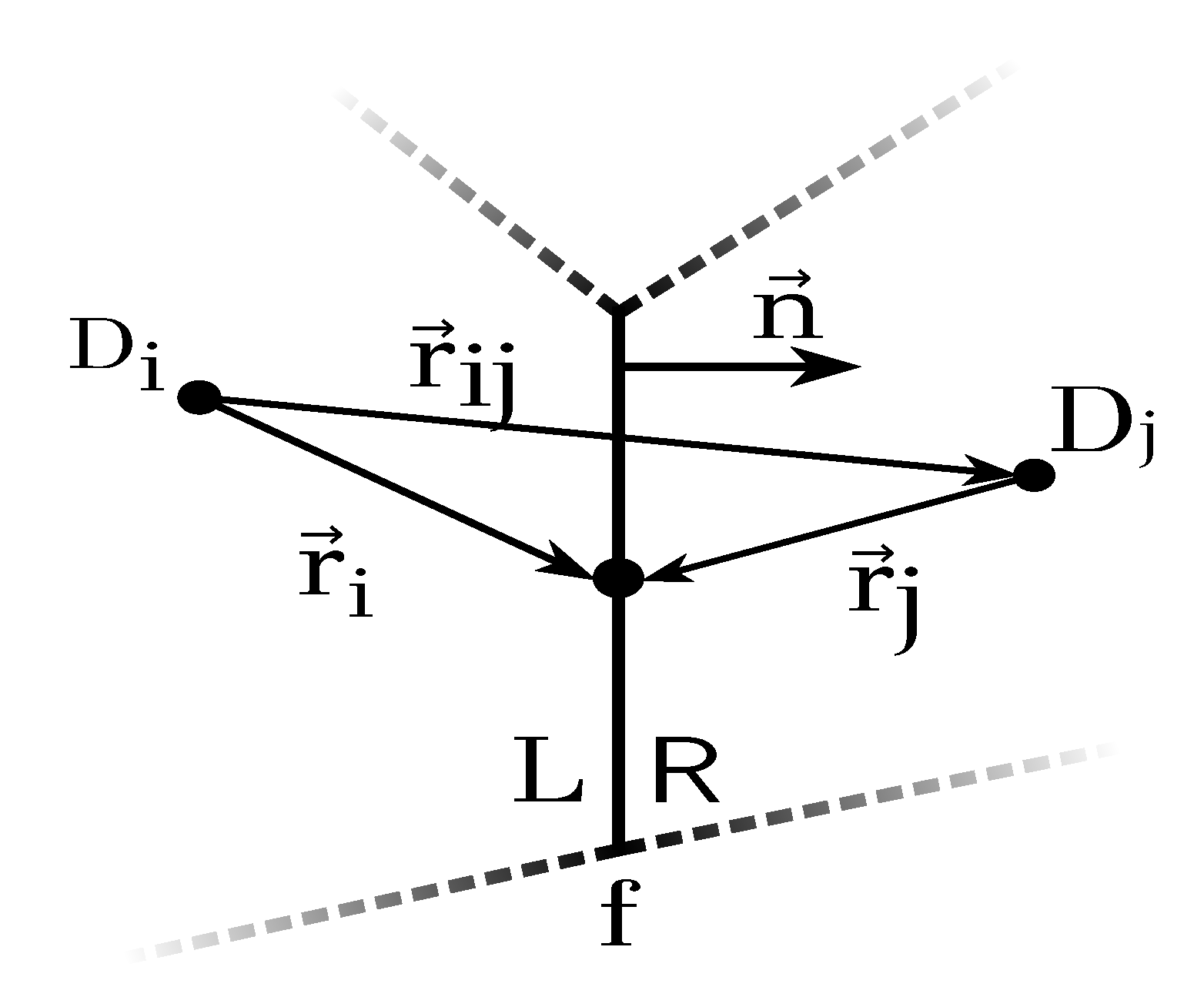
The evaluation of the inviscid fluxes in Equation (10) requires an approximation of the left and right state of a face (Figure 1). These states are computed based on a reconstruction scheme that extrapolates the cell-centered value of the volumes in the respective face. The right and left state are designated based on the normal vector of the face, which points from the left state to the right. Due to the particular nature of the governing equations, a different reconstruction scheme is adopted for each equation.
The velocity field is approximated through a piecewise linear interpolation scheme, given by Equation (12). Since the surface tension is neglected, the velocity field is continuous even across the free surface. For this reason, the gradients are retained, and no limiter is applied.
The vectors are pointing from the cell center to the midpoint of the face, as illustrated in Figure 1.
Furthermore, the pressure field is a continuous function in space, since surface tension is neglected. However, the pressure gradient is discontinuous across the free surface, due to the density jump. The jump condition that must hold requires . Many researchers [17,31] have introduced different schemes to treat this difficulty by adopting a density-based interpolation scheme. In MaPFlow, the work of Queutey et al. [17] is followed. This scheme is introduced only near the free surface, while in the rest of the computational domain a piecewise linear interpolation scheme is used, similar to Equation (12).
Finally, of great importance is the reconstruction of volume fraction field (). In order to reduce the numerical diffusion, it is important to adopt a compressive reconstruction scheme. Over recent decades, numerous reconstruction schemes have been introduced which offer low numerical diffusion. The requirements should meet is boundedness and high accuracy even in large CFL numbers. Most of these reconstruction schemes are based on Leonard’s Normalized Variable Diagram (NVD) [32] (e.g., CISCAM [33], HRIC [34], BICS [35]). In the present work the STACS [36] scheme is adopted as the free surface capturing scheme.
3.2. Temporal Discretization
The present section focuses on the time discretization process. Let be the vector of unknowns. An implicit formulation of the problem can be defined as
where is the unsteady residual (14), which includes the spatial terms of Equation (7), here denoted as , and the unsteady term.
If n is the index of the known time solution and k is the internal iterator of the steady problem, then at the beginning of every steady iteration , the vector of unknowns is initialized as and until convergence they do not satisfy the original unsteady problem. The convergent solution of the problem is obtained when and hence .
The unsteady term is discretized as a series expansion of successive levels backwards in time (BDF schemes) [37].
When the control volume changes in time, the Geometric Conservation Law (GCL) [38] should be satisfied (Equation (16)).
Using a similar backwards differentiation in time as in Equation (15) the GCL can be written as
where the residual of the GCL is defined as
To ensure that the GCL is satisfied, Equation (17) is applied directly to the discretization of the unsteady term and thus Equation (15) becomes
In MaPFlow two successive levels of solution are retained, yielding a second order accurate scheme in time. The fictitious time derivative of equation is discretized using a first-order backward difference scheme
To facilitate convergence the local time stepping technique is used. The local pseudo-timestep is determined by
where is the convective spectral radii and it is defined by
3.3. Turbulence Modeling
Regarding turbulence modeling, the SST model of Menter [39] is used in this work. A well-known downside of RANS models when employed for free surface flows is the exponential growth of the turbulent kinetic energy and eddy viscosity [40,41]. The overproduction of turbulence viscosity, especially around the interface between water and air, is triggered by the shear layer in the free surface and results to an artificial damping of the propagated waves. Devolder et al. [40] proposed a buoyancy term (23) to the turbulent kinetic energy equation.
3.4. Wave Generation and Absorption
When considering a numerical wave tank, the generation of the desired wave profile as well as the effective radiation of the outgoing waves outside the computational domain are two non-trivial tasks. The generation of steadily progressive waves is performed by forcing the numerical solution, in a specific part of the computational domain, to follow a wave solution provided by a wave theory. Furthermore, an artificial damping of the waves is required near the boundaries of the domain. The boundary conditions, assume a uniform field and thus any physical disturbance created inside the domain should not reach the farfield boundary. Various techniques have been considered for practical implementations. Among them, is the coarsening of the computational mesh near the boundaries. Although this technique is able to smear the solution, the mesh coarsening is case-dependent, and it does not guarantee zero reflection. In most cases, the boundaries are supplied with damping zones where the farfield conditions are imposed.
In this work, the numerical generation and absorption of the free surface waves is performed through source terms applied in the momentum equations, in specific zones of the computational domain near the farfield boundaries. Typically, these zones extend for a few wavelengths. The general form of the source terms is given by Equation (24). This source term drives the solution to the imposed velocity vector.
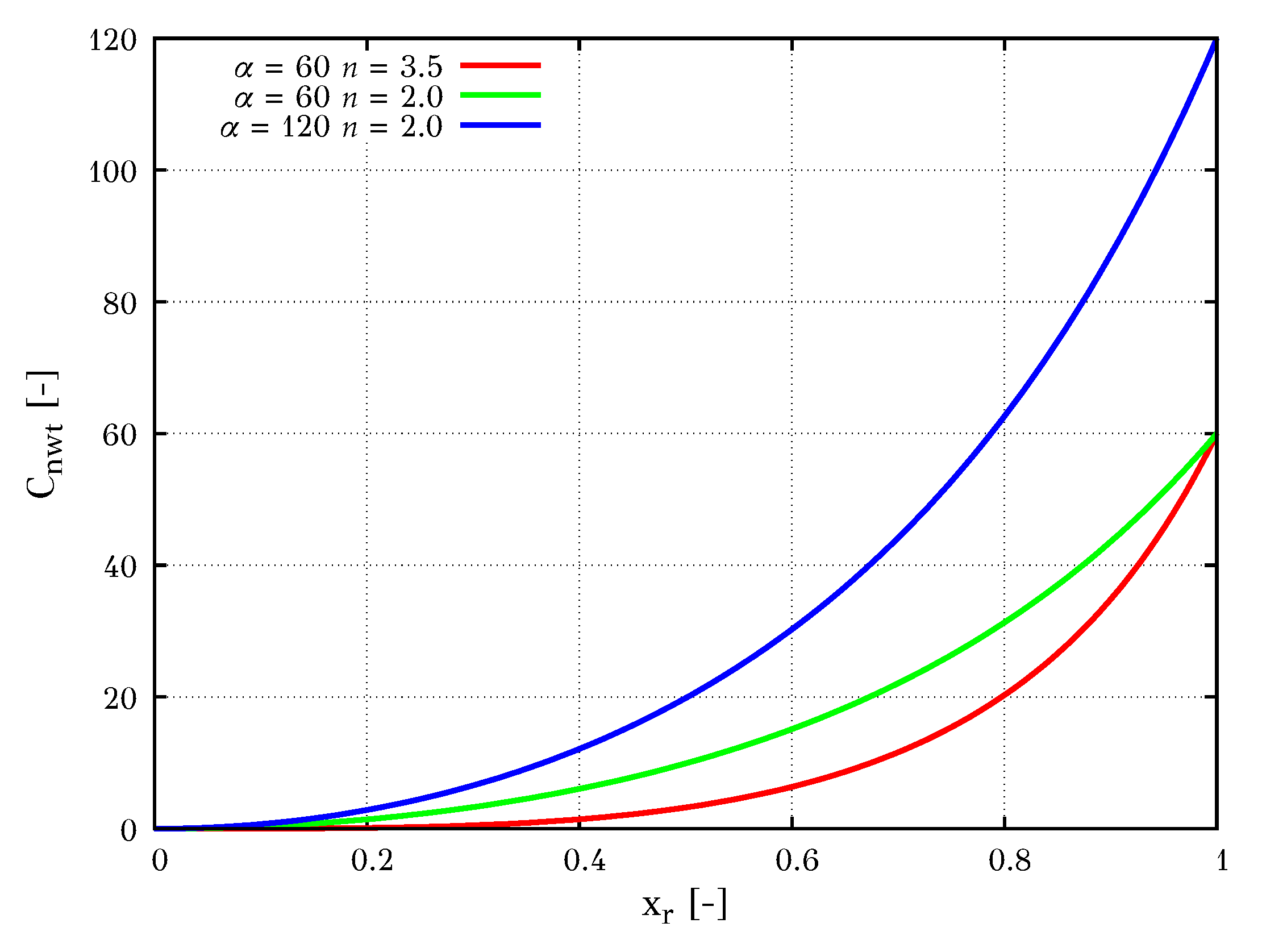
The effect of the source terms is regulated through the function, its form is given by Equation (25), while in Figure 2 it is plotted for different values of and n. The maximum value of the function is regulated through parameter , while its spatial distribution through n parameter. The function is zero away from the boundaries of the computational domain, scales exponentially inside the specified zone and it reaches its maximum value at the boundary. This function was originally proposed in [43] where the desired numerical solution was imposed explicitly. In the present work, the desired numerical solution (e.g., a specific wave profile in the generation zone) is obtained implicitly, meaning that the solver needs to converge to that solution through the numerical procedure. The source term (25), should be able to drive the solution to the desired one, while at the same time maintain the convergence properties of the method. Large values of may lead to numerical instabilities, while small values of may not be able to drive the solution. Typical values for the exponent n is between 2 and 5 and usually multiplier is not greater than 200. In the first section of the numerical results, it will be shown that there is an acceptable range of values for the coefficient where no numerical instabilities appear.
The source term of Equation (25) is a function of the non-dimensional space variable , which depends on the starting position of the specified zone and the end point of the zone .
The wave generation is performed by imposing the velocity as given by an appropriate wave theory. In this work, the wave solution is obtained from the semi-analytical method of Fenton’s Stream Function Theory [44].
In case of the wave damping zones, the target is to minimize the transverse velocity components. In a two-dimensional context, where the wave propagation is along the x-axis, the velocity vector takes the form . This method has been assessed extensively as a wave damping technique [45]. In the present work, wave generation is accomplished in a similar manner.
3.5. Volume Fraction Boundedness
The volume fraction equation is an advection equation. The values of should always remain inside the definition bounds . However, due to numerical instabilities its value may surpass its domain of definition. This can be triggered by two factors. First, for the derivation of the conservative form of the VOF equation a divergence free field was assumed. This may not hold when distorted meshes are used, near the sharp edges of the wall boundary or when dominant sources are applied (such as in damping and generation zones). Secondly, another reason for violating the domain of definition is the spurious oscillations caused by the reconstruction scheme of the VOF field. High order reconstruction scheme may introduce unphysical oscillations near sharp discontinuities [46]. This may be treated by employing a first-order approximation which would ensure boundedness, but at the cost of excessive diffusion. Much work has been done to remedy this behavior, especially in the frameworks of the Total Variation Diminishing (TVD) schemes [47] and of the Normalized Variable Formulation [32]. Unfortunately, in practical implementations the requirements for boundedness of the reconstruction scheme may not be satisfied. Finally, it should be noticed that both arguments are correlated with the timestep resolution and thus small Courant number are usually adopted.
In MaPFlow a relaxed limit (of order ) to the volume fraction is applied. Through numerical investigation it was seen that the VOF clipping was large during the initial stages of simulations; however, when a steady or periodic state was reached the clipping was reduced significantly. In all cases, the introduced mass error was negligible.
4. Numerical Results
In this section, numerical results based on the artificial compressibility method are presented. First, the ability of the solver to accurately generate and propagate waves on constant bathymetry is demonstrated. Following a grid and timestep sensitivity study, a parametric study regarding the influence of the artificial compressibility parameter is presented. Afterwards, the interaction of waves with variable bathymetry is considered and the results are compared with experimental data. Finally, a two-dimensional fluid–structure interaction problem is presented. In the latter case, the artificial compressibility methodology is coupled with a dynamic solver and the interaction of moonpool-type floater with incident waves is examined. The amplitudes of the motions are compared with experimental data.
4.1. Numerical Wave Tank
The propagation of a cnoidal wave at constant bathymetry is considered. The wave period is equal to s, the wave height is m, while the depth of the numerical wave tank is m. Using the stream function theory of Fenton, the wavelength is found equals to m.
4.1.1. Wave Generation and Absorption
First, the influence of the generation parameters , as defined in Equation (25) is investigated. In Table 1 six test cases are defined. The same grid configuration is used in all cases. In the direction of the wave propagation, the mesh is uniform almost everywhere with 150 cells per wave period, except in the damping zone where the mesh coarsens based on a geometric rule. In the vertical direction, 20 cells per wave height are employed. Regarding the timestep discretization, a constant timestep is chosen corresponding to 800 timesteps per wave period ( s).
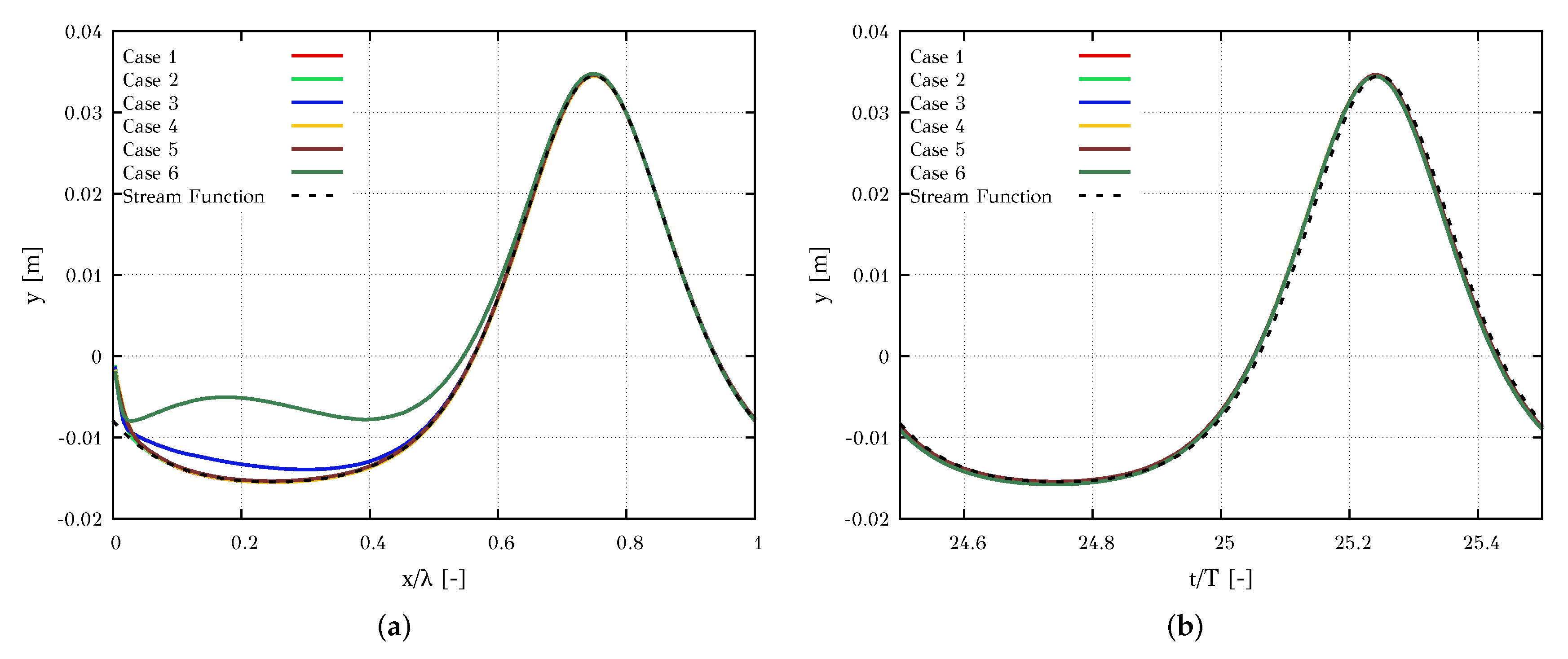
The surface elevation, for all cases, inside the generation zone are shown in Figure 3a and is compared with the analytical solution provided by the Stream Function Theory. It can be seen that the waveform is distorted for large values of . Furthermore, discrepancies are noted near the farfield boundary. This occurs due to a lagging between the boundary conditions and the time window that solver need to converge to the imposed wave solution. However, in all cases the solution converges to the desired wave profile as depicted in Figure 3b, where the free surface elevation is plotted against time and it is compared with its analytical form.
Table 2 and Table 3 present the error of the amplitude of the first four harmonics and the error of the phase angle in degrees between the analytical and numerical solution. Overall, the error of the amplitude at the dominant frequency is below 0.5% for all cases, while for large values of an amplification in higher frequencies is evident. The exponent n does not seem to have any significant influence on the results. The general recommendation is that the source terms should have small influence in the system of equations, in order to enhance the stability of the solver. For this reason, large values of exponent n and small values of the parameter are desired. On these grounds, an accurate representation of the wave profile is obtained, while keeping the influence of the source terms small, by choosing and .
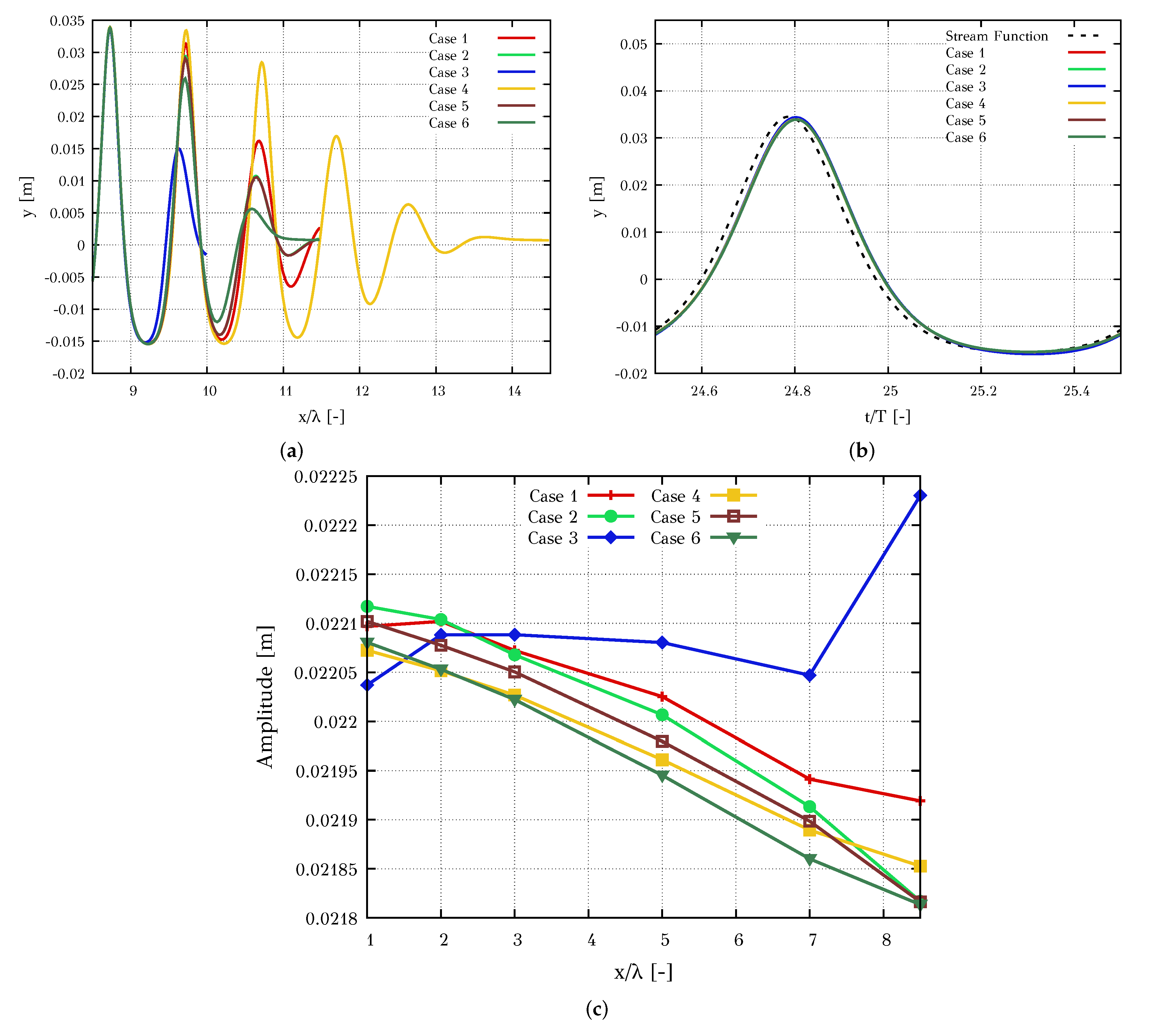
Next the damping performance of the solver is evaluated. A parametric study is conducted by varying the values of the parameters , n and the length of the damping zone. The case studies are defined in Table 4. The asterisk, in the last two cases, indicates that the damping zone is coarser. In Figure 4a the surface elevation inside the damping zone is shown for the six test cases, while in Figure 4b the free surface elevation during a wave period at the beginning of the damping zone is presented. As illustrated in Figure 4a, the elevation of the free surface near the boundary is completely damped in case 4, contrary to cases 1 and 3. It is also worth noticing that for the same parameters , n (cases 2 and 5) the grid coarsening does not affect the damping of the wave. However, all cases produce the same wave profile at the beginning of the damping zone.
Furthermore, in order to examine in detail the effect of the damping zone in the wave flume, the amplitude of the 1st harmonic of the free surface elevation is plotted in Figure 4c, at various stations across the computational domain. As expected, in all cases the amplitude decays due to numerical diffusion. However, in case 3 an oscillatory behavior of the harmonics amplitudes is noticed. This is caused by reflections at the boundary of the domain. Also, in case 1 the amplitude of the 1st harmonic is not monotonically decreasing in space. This can be attributed to reflections at the farfield boundary, as in the previous case. In all other cases, the differences are regarded negligible. A damping zone extending six wavelengths is excessive for practical implementations while large values of may cause numerical instabilities. For this reason, is chosen (case 2) for the rest of the work.
Most of the results showed that the generation and damping technique can produce accurate results. The differences noted for different values of and n can be considered small. In case of wave generation, the numerical procedure was able to provide acceptable results in all cases however for large values of (>300) numerical instabilities were noticed. Regarding wave damping, the method can absorb the outgoing waves, provided that the length of the zones is sufficient. Finally, the damping sensitivity study indicates that the damping performance is more sensitive to the chosen value of . For this reason, a larger value of , compared to wave generation, is chosen.
4.1.2. Grid and Timestep Independence
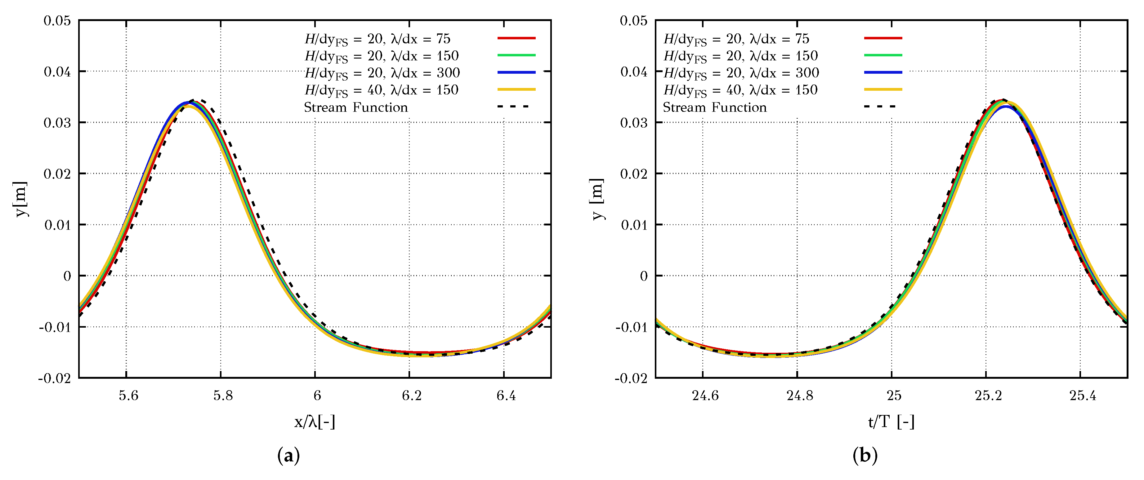
Once and n are decided the next step is to perform a grid and a timestep sensitivity study. The grid parameterization is based on the number of cells per wavelength () and the number of cells per wave height near the free surface (). Predictions from four grids are compared in Figure 5 with respect to free surface elevation in Figure 5a and the elevation at a specific station during a wave period in Figure 5b.
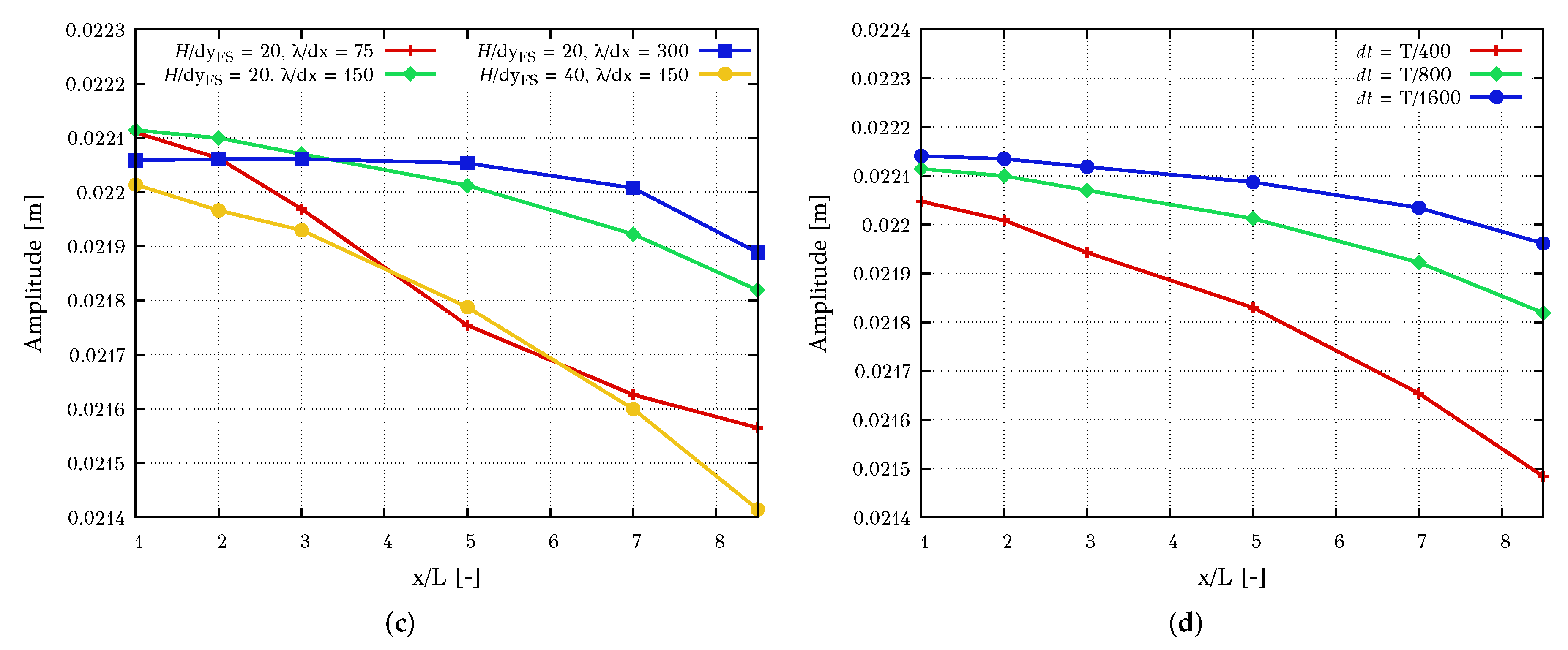
In Figure 5c the amplitude of the first harmonic of the propagating wave is depicted. The figure shows that in case of the fine grid (blue line) the amplitude of the wave elevation remains almost constant across the domain. The coarse grid (red line) produces significant numerical diffusion and the amplitude of the waves is decreasing. The yellow line corresponds to a mesh with highly skewed cells near the free surface. It should be noticed that although the green line corresponds to a coarser grid, the numerical diffusion introduced is smaller. Due to very thin cells near the free surface, the CFL number is large and consequently the numerical diffusion introduced by the temporal discretization is significant [48]. The computational mesh with 150 cells per wavelength and 20 cells in the wave height (green line) exhibits similar characteristics with the finer grid (blue line) and consequently, it is kept for the rest of the simulations.
In Figure 5d the amplitude of the first harmonic of the cnoidal wave can be found. Three different timesteps are considered, based on the wave period. Predictions for 400, 800 and 1600 timesteps per period are shown. It is evident that that even when 400 timesteps per period are chosen the relative error after 8 wavelengths is . Predictions with 800 and 1600 timesteps per wave period are in very close agreement and thus the former is selected in the present work.
4.1.3. Influence of the Artificial Compressibility Parameter
The next case is to study the impact of the artificial compressibility parameter on wave propagation. In general, regulates the coupling between pressure and density during convergence, i.e., regulates the pseudo-sound speed (c). On the one hand, small values of lead to small values of c thus the system is strongly coupled, on the other hand large values of lead to a loose coupling of the equations. Because the parameter affects the convergence of the method, it is imperative to quantify how the choice of affects the predictions.
Several guidelines for choosing can be found in the literature. For one-phase incompressible flows, Turkel [22] proposed that should scale with the square of the local velocity, and hence varies across the domain. Special care should be taken near stagnation points where its value should be safeguarded. In case of wave propagation, the velocities under the crest are small and so the parameter could not depend on the local characteristics of the flow. Nevertheless, the flows considered in his work did not involve gravity. Kunz et al. [24] applied the AC method for cavitation problems and suggested values of ranging from . In order to understand the effect of on the predictions, we conduct a parametric study, using five different constant values of 1, 10, 50, 100 and 1000.
The numerical setup is based on the previous remarks. The results are summarized in Figure 6. Figure 6a shows the free surface elevation 5 wavelengths downstream of the generation zone. It is evident that the predictions yield large differences for the two extreme values of ( and ). However, for values ranging from 10–100 the predictions yield negligible differences. This is also exhibited in Figure 6b where the amplitude of the first harmonic for the various values is shown. For values and elongation of the wavelength is observed. This is an artifact that implies undesired compressibility effects.
To further investigate the effect of on the solution, the 2nd and 3rd harmonics are provided in Figure 6. It is apparent that within the range the solution is insensitive to the chosen value for both the 2nd (Figure 6c) and 3rd (Figure 6d) harmonic. Nonetheless, for the differences are larger but still within an acceptable limit. For the solutions is clearly affected.
From the preceding analysis, it is evident that for the present formulation predictions are insensitive of value of within an acceptable range. With these considerations and taking into account the guidelines of the literature, a value of is chosen for the rest of this work.
4.2. Wave Interaction with Variable Bathymetry
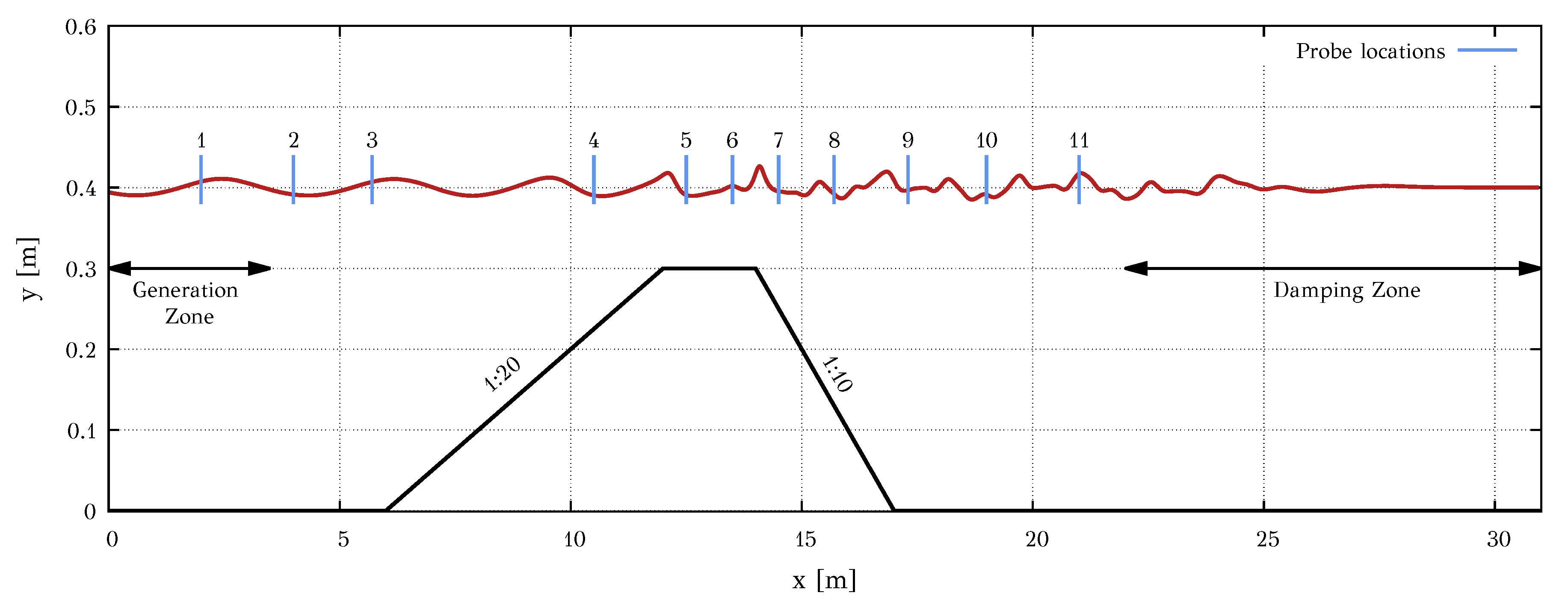
We shall now consider the interaction of a wave with a trapezoidal bathymetry. This is a standard benchmark to evaluate the solver’s capability to accurately simulate dispersive phenomena. The original experiment was setup and conducted by Beji and Battjes [49], where seven wave gauges were placed along the wave tank. Later, Dingemans [29] repeated the same experiment using four more probes. The location of the wave probes are depicted in Figure 7. The generated wave profile has height cm and period s.
Figure 7 also illustrates the numerical setup. The length of the numerical wave tank is 31 m. The damping zone is 9 m and the wave generation zone extends for m. The coefficients of the generation and damping zones are chosen according to the preceding investigation. Following the guidelines from the previous analysis, a timestep and grid sensitivity study was conducted. The timestep resolution was based on the incident wave period, and the parametric study included the values and . The spatial mesh should have enough resolution to account for the smallest ripples of the irregular wave caused by the interaction with the bathymetry. The sensitivity study concluded for the timestep resolution to es which corresponds to ≈800 steps per period and to a grid of total size of cells. The grid in the x direction is uniform with mm, in the y direction the mesh is dense near the free surface ( mm) and coarsens gradually towards the bottom.
Regarding the numerical setup, the artificial compressibility factor is equal to . The pseudo-CFL number is equal to 50 and at each time true iteration 10 dual steps were executed for the convergence of the pseudo-steady state problem. At the bottom, no slip boundary condition is applied.
The predicted free surface elevation is also presented in Figure 7 (continuous red line). Due to shoaling, the wavelength is compressed, and energy is transferred to higher harmonics. The deepening after the bar releases the energy from the higher harmonics and an irregular wave profile is obtained.
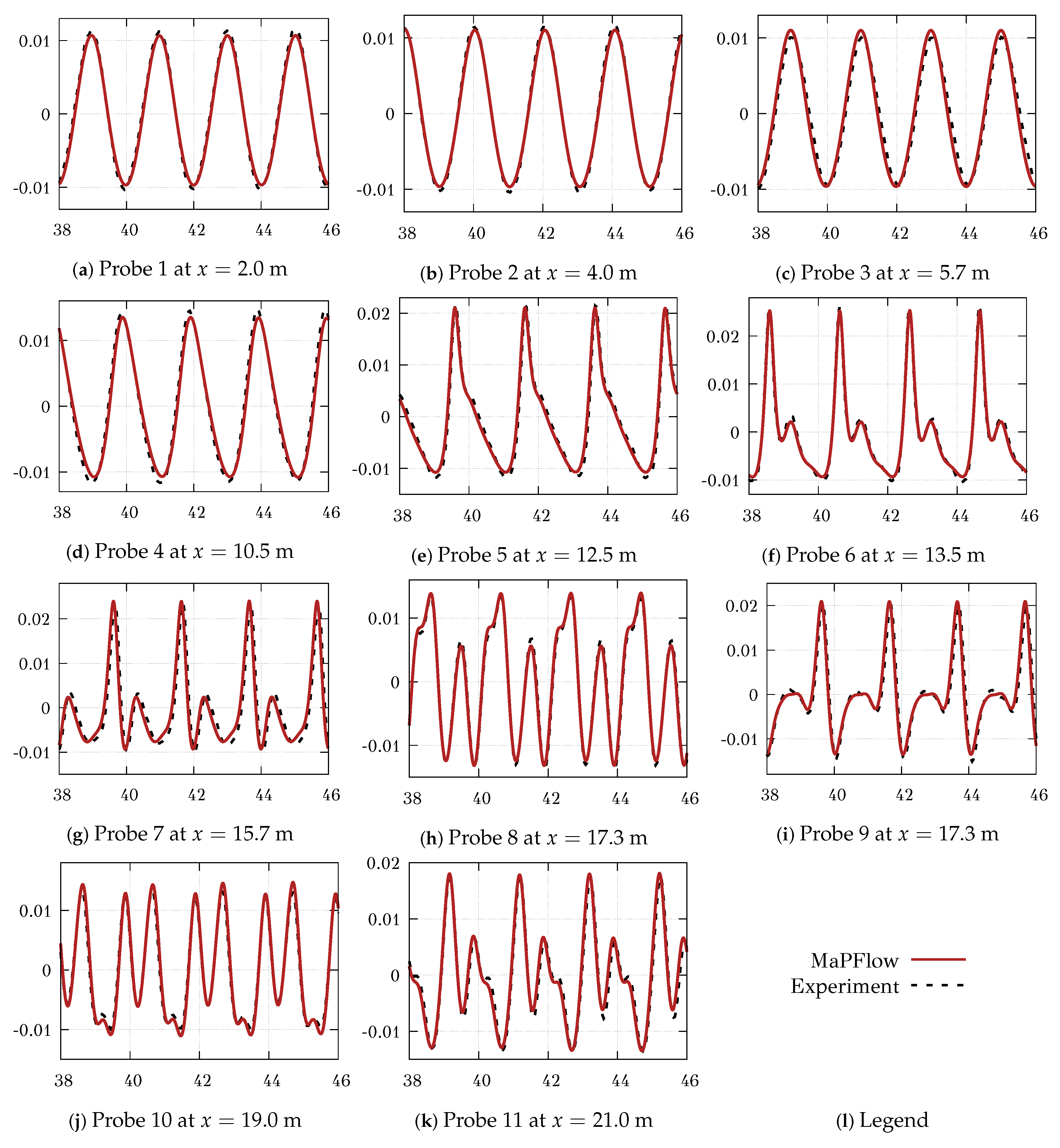
The signals recorded at the wave probes are compared against the experimental data in Figure 8, at eleven stations.
At the first probe (Figure 8a), the two signal appear to have a small difference in amplitude. However, as the comparison at the other probes suggests it does not affect the overall comparison. At probe 7 (Figure 8g) a small phase shift is observed between the simulation and the measurements. Nevertheless, the comparison of free surface displacement is very good at all stations even when higher harmonic are excited after the shoaling (Figure 8f–k).
4.3. Moonpool-Type Floater
In this section, the response of a moonpool-type floater in incident wave is investigated and compared with experimental data from [30]. Under wave excitation the floater is displaced and the free surface inside the moonpool is subjected to a vertical motion, commonly called piston motion, while additional sloshing modes may appear. The piston motion inside the moonpool reduces the motion of the structure induced by the incident waves. This problem poses additional challenges since the motion of the floater is induced by the underlying flowfield. It is noted that viscous effect are significant in this case since the flow separation at the sharp edges directly affects the free surface elevation inside the moonpool. Employing potential methods in this case results in overshoots of the piston mode and thus viscous corrections must be included [50,51].
The motion of the floater is described by Newton’s second law. At each unknown timestep , Equation (26) should be satisfied.
The vector contains the unknown displacements and rotations and the double dots imply twice differentiation with respect to time. The matrix M is the mass matrix and vector includes the sum of the forces applied to the body (e.g., hydrodynamic forces, external forces, etc.). The above system of equations constitutes a non-linear system of equations. A linearization is imposed based on the assumption of small perturbations in each pseudo-timestep. As a result a linearized -formulation is obtained (Equation (27)).
In the above equation is the force vector calculated at the known timestep k and for the correction applies .
This linearization implies an iterative process during pseudo-timesteps. At each k-iteration the correction components are computed based on the hydrodynamics forces provided by the solver. The iterative procedure ends when both solvers converge, implying a strong coupling between them.
The second order ordinary differential equations (ODE) (27) are solved with the Newmark- method with coefficient values and . This method uses a second order Taylor expansion variant, in which a predictor step is intervened based on the coefficients and .
Since the geometry, is not stationary an appropriate grid technique needs to be adopted to account for the moving boundaries. In cases of small amplitude motion, the deforming grid technique could be used. In MaPFlow the nodes of the mesh are moved based on a damping term as described in [52].
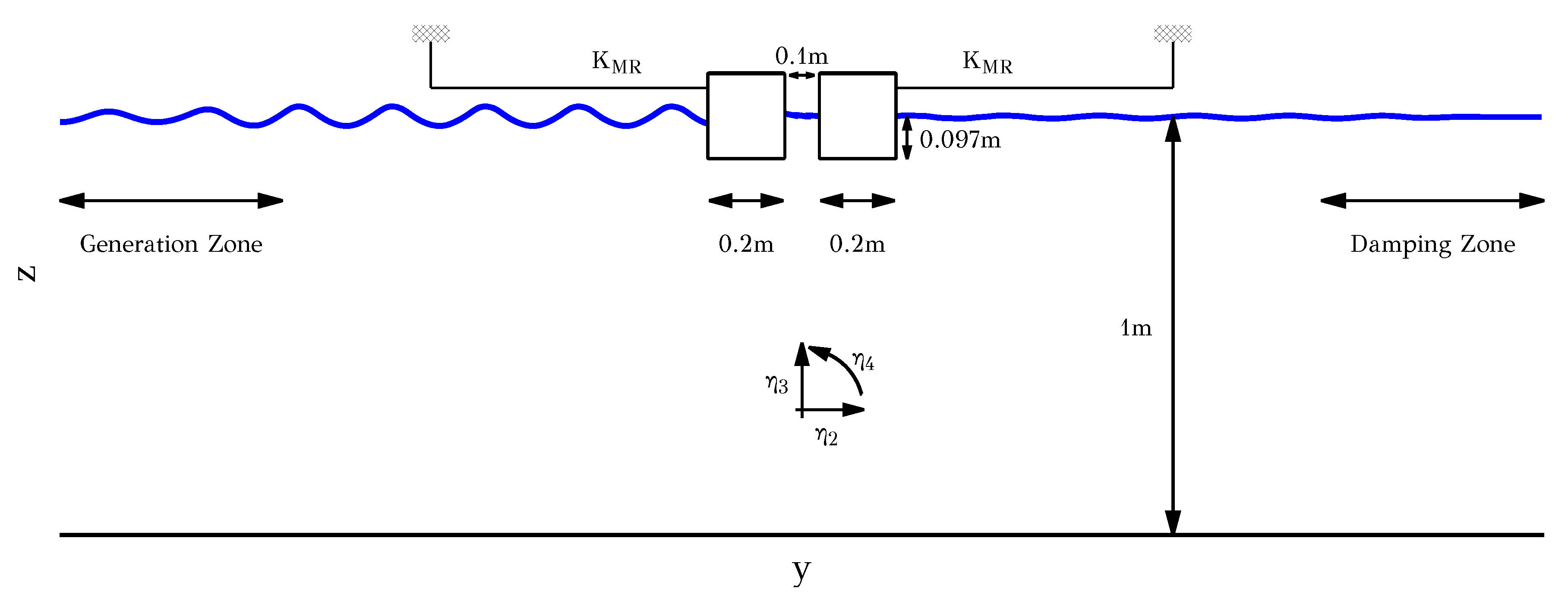
In the experiments conducted by [30] two barges of rectangular cross section of 20 cm were mounted together to form a moonpool of 10 cm. The breadth of the barges was 14 mm smaller than the width of the experimental wave tank and thus 3D effects are limited.
Following the notation of the experiments, the test case is defined on the y–z plane. In a two-dimensional context, a body has three degrees of freedom, namely the sway motion (motion along the y-axis, ), the heave motion (motion along the z-axis, ) and the roll motion (motion around the x-axis, ).
The setup of the experiment is depicted in Figure 9. The structure is mounted with horizontal mooring lines to prevent it from drifting. At the end of these lines springs were connected to allow the structure to move. Pre-tension was applied to the springs, which was much larger than the tension due to motion, thus the restoring effect of the mooring system was always active. A coupling between sway and roll motion is assumed because the center of gravity of the model and the mounting point of the mooring lines were not in the same height. Considering the abovementioned remarks, the rigid body motion is described by Equations (28).
In the above equations m is the mass of the structure, I is the inertia of momentum about its center of gravity, is the normal unit vector defined on the boundary S of the body, the components of , p is the fluid pressure and is the viscous stress tensor. Lastly, and are the spring constants for the heave and roll motion, respectively and are the spring constants for coupling of the heave and roll motion due to the level arm formed between the axis of the restoring forces and the center of gravity. A more detailed report for the experimental setup and the physical modeling of the rigid body motion can be found in [53].
The experiment considered three types of waves based on the wave height to wavelength ratio for several wave periods. In the present study, only results for waves with ratio for wave periods between the range are presented.
The flow is considered fully turbulent for all wave periods. This is valid for a large amplitude of motion, where wave-breaking occurs. In smaller amplitudes, the production of turbulent viscosity is lower resulting in an almost laminar approximation. The grid and the timestep is the same for all cases. In the stream-wise, direction the grid is almost uniform with size of m and in the transverse direction in the near free surface regime m. On the damping zone region, the mesh coarsens with a geometric rule to effectively damp the outgoing waves. The grid around the structure has an O-grid topology which is dense to account for the vortex formation near the sharp edges. The total size of the mesh is cells. Based on a sensitivity study, the timestep is selected equals to s.
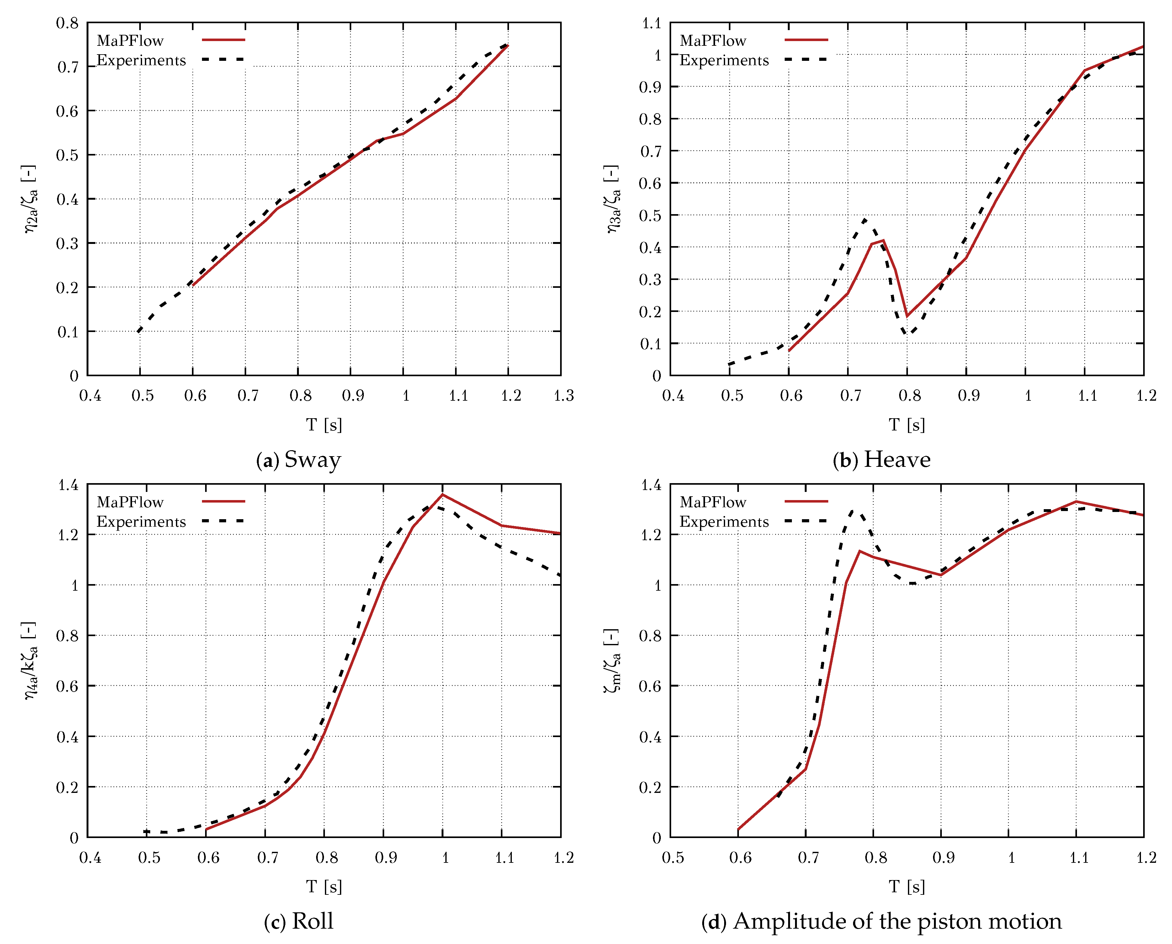
In Figure 10 the results are compared with the experimental data. In Figure 10a–c the Response Amplitude Operators (RAOs) of the motions are presented, while Figure 10d presents the amplitude of the space averaged free surface elevation inside the moonpool. Regarding the sway motion, the amplitudes scale linearly with respect to the wave period and the results coincide with the experimental ones. The heave amplitudes appear to have a resonant behavior for wave periods between s and s. This behavior is depicted in the amplitudes of the free surface as well. Small discrepancies are observed near this resonant region. Furthermore, the Figure 10c shows the amplitudes of the roll motion, except for large wave periods the present method produces similar results with the experiments. However, larger amplitudes of roll motion are obtained for wave periods between s and s. This could be caused due to the assumption of two-dimensional flow. Additional drag forces could be act on the structure caused by the liquid between the side of the structure and the wave tank.
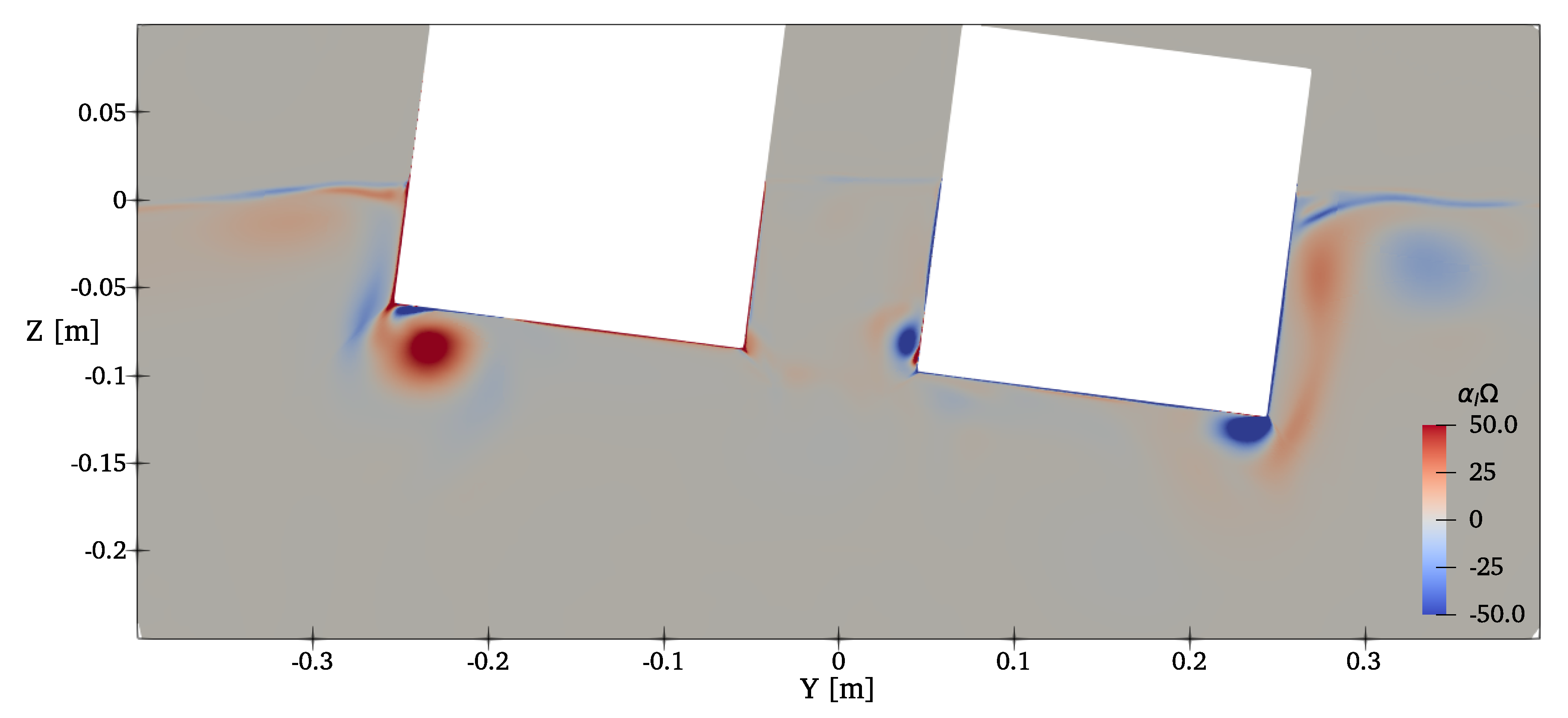
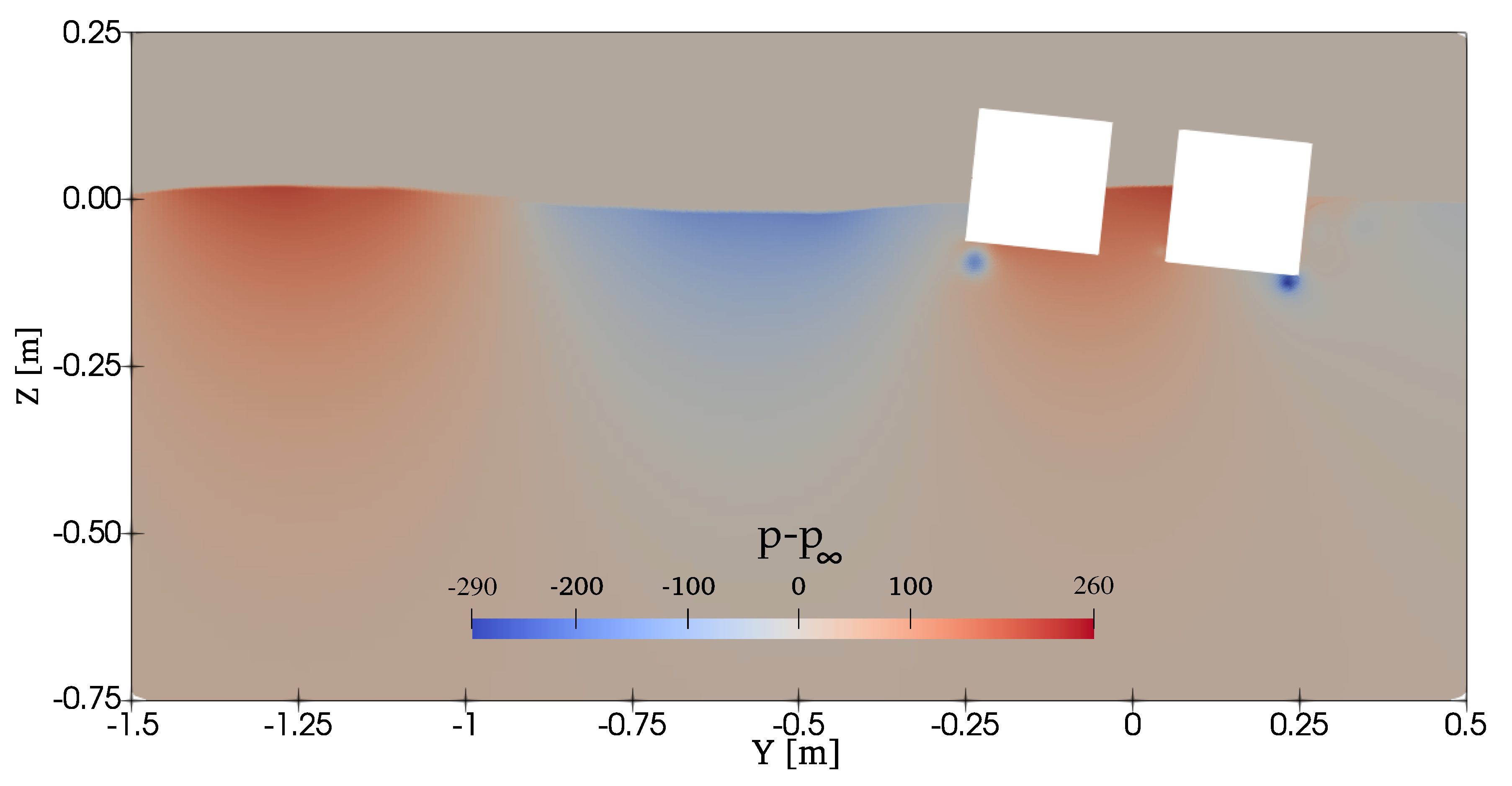
In Figure 11 vorticity near the edges of the structure is depicted where the flow separation at the corners of the structure is evident. The flow separation at the lower entrance of the moonpool regulates the resonant behavior of the piston mode which is apparent for wave periods between s and s. Finally, the pressure field upstream of the structure is presented in Figure 12. The figure illustrates the pressure distribution at the incident wave, the free surface elevation inside the moonpool, as well as the pressure drop due to vortex formation near the sharp edges of the structure.
5. Conclusions
Concluding, in the present work a two-phase flow solver was formulated based on the artificial compressibility approach and the volume of fluid method. In the first part, the derivation of the hyperbolic system of equations was presented. A detailed analysis of the time discretization process was illustrated, while emphasis was given to account for the moving boundaries. Regarding the spatial discretization the finite volume method was used, while an approximate Riemann solver was used for the evaluation of the inviscid fluxes. Finally, a simple and efficient implicit methodology to generate and absorb free surface waves was illustrated.
A series of numerical test cases was performed to demonstrate the efficiency and consistency of the solver. A simple wave propagation problem on constant bathymetry was chosen to illustrate the ability of the solver to generate, propagate and damp free surface waves. Also, the same configuration was used to investigate the effect of the artificial compressibility parameter-. The results indicate that there is a wide range of values where no significant differences were observed. Regarding the last two validation examples, the predictions of the solver were compared to available experimental data. In case of the variable bathymetry the solver was able to perform well and account for the higher harmonics developed due to shoaling.
In the final test case, it was shown that the present methodology was able to produce adequate results for a surface piercing problem with wave–structure interaction. The solver was able to handle the fluid–structure interaction problem accurately being in close agreement with the measurements.
As a last remark, the proposed methodology compared to the alternatives provided by the literature solves a single system of equations in a coupled manner. The formulation enables simulation of free surface flows using a hyperbolic perspective. The method performed well in a variety of cases, providing a viable alternative for modeling free surface flows within the CFD framework.
Author Contributions
Both authors contributed equally. Both authors have read and agreed to the published version of the manuscript.
Funding
This research received no external funding.
Acknowledgments
MaPFlow computations were supported by computational time granted from the Greek Research and Technology Network (GRNET) in the National HPC facility—ARIS—under project “WAVEMAP” with ID pr008051_thin.
Conflicts of Interest
The authors declare no conflict of interest.
Appendix A. Discretization of the Hyperbolic System of Equations
The equations of flow (7) are discretized-based on the finite volume method. Control volumes are defined in every cell of the mesh with its center being the geometric center of the mesh elements. The unknown variables are expressed over a control volume as
The surface terms of Equation (7) are considered constant in each face of the control volume. Thus, the surface integrals are approximated through a sum of surface terms evaluated at the midpoint of every face. Furthermore, the volume terms are considered constant in each . As a result, the spatial terms are computed based on the following equation.
The inviscid fluxes are computed through the approximate Riemann solver of Roe [54]. As mentioned in Section 2, the eigenvalues of the inviscid Jacobian depend on the density field. For this reason, the preconditioned matrix is used in the evaluation of fluxes. The preconditioned Jacobian is defined as
where is the preconditioned matrix (9) and is the inverse matrix. The matrix is given by Equation (A4).
The convective fluxes are computed, at a face f, using the Roe approximate Riemann solver as
The indices denote the right and the left state of the face, as defined by the normal vector. The Jacobian matrix is computed based on the absolute values of the eigenvalues of the system. Specifically, let be the matrix constructed by arranging the left eigenvectors of in a column wise order, be the matrix constructed by arranging the right eigenvectors in a row wise order and be the diagonal matrix constituted by the absolute values of the eigenvalues, then the Jacobian matrix can be written as
The inviscid Jacobian of Equation (A6) is computed based on the Roe averaged quantities at face f, given by (A7).
The eigenvalues of the Jacobian matrix are given by Equation (A8). The eigenvalues have similar form as in the case of the compressible equations. The difference is the pseudo-sound speed does not depend on the flow characteristics, but on the choice of parameter and the hyperbolic definition of the equations is valid only during pseudo-time iterations.
In previous equations, c is the artificial sound speed, where in case of two-phase flows, is defined as
In the preceding equations , and are expressed as
while for the unit vectors and should hold .
References
- Grilli, S. Fully nonlinear potential flow models used for long wave runup prediction. In Chapter in Long-Wave Runup Models; Yeh, H., Liu, P., Synolakis, C., Eds.; World Scientific Pub Co Pte Lt.: Singapore, 1997; pp. 116–180. [Google Scholar]
- Filippas, E. Hydrodynamic Analysis of Ship and Marine Biomimetic Systems in Waves Using GPGPU Programming. Ph.D. Thesis, National Technical University of Athens, School of Naval Architecture and Marine Engineering, Zografou, Greece, 2019. [Google Scholar]
- Manolas, D. Hydro-aero-elastic Analysis of Offshore Wind Turbines. Ph.D. Thesis, National Technical University of Athens, School of Mechanical Engineering, Zografou, Greece, 2015. [Google Scholar]
- Papoutsellis, C.; Athanassoulis, G. A new efficient Hamiltonian approach to the nonlinear water-wave problem over arbitrary bathymetry. arXiv 2017, arXiv:1704.03276. [Google Scholar]
- Filippas, E.S.; Papadakis, G.P.; Belibassakis, K.A. Free-Surface Effects on the Performance of Flapping-Foil Thruster for Augmenting Ship Propulsion in Waves. J. Mar. Sci. Eng. 2020, 8, 357. [Google Scholar] [CrossRef]
- Takizawa, A.; Koshizuka, S.; Kondo, S. Generalization of physical component boundary fitted co-ordinate (PCBFC) method for the analysis of free-surface flow. Int. J. Numer. Methods Fluids 1992, 15, 1213–1237. [Google Scholar] [CrossRef]
- Tzabiras, G.D. Resistance and Self-Propulsion Simulations for a Series-60, CB = 0.6 Hull at Model and Full Scale. Ship Technol. Res. 2004, 51, 21–34. [Google Scholar] [CrossRef]
- Hirt, C.; Nichols, B. Volume of Fluid (VOF) Method for the Dynamics of Free Boundaries. J. Comput. Phys. 1981, 39, 201–225. [Google Scholar] [CrossRef]
- Sussman, M.; Smereka, P.; Osher, S. A level set approach for computing solutions to incompressible two-phase flow. J. Comput. Phys. 1994, 114, 146–159. [Google Scholar] [CrossRef]
- Harlow, F.H.; Welch, J.E. Numerical calculation of time-dependent viscous incompressible flow of fluid with free surface. Phys. Fluids 1965, 8, 2182–2189. [Google Scholar] [CrossRef]
- Vukcevic, V. Numerical Modelling of Coupled Potential and Viscous Flow for Marine Applications. Ph.D. Thesis, Fakultet Strojarstva i Brodogradnje, Zagreb, Croatia, 2017. [Google Scholar] [CrossRef]
- Plumerault, L.R.; Astruc, D.; Villedieu, P.; Maron, P. A numerical model for aerated-water wave breaking. Int. J. Numer. Methods Fluids 2012, 69, 1851–1871. [Google Scholar] [CrossRef]
- Liu, S.; Gatin, I.; Obhrai, C.; Ong, M.C.; Jasak, H. CFD simulations of violent breaking wave impacts on a vertical wall using a two-phase compressible solver. Coast. Eng. 2019, 154, 103564. [Google Scholar] [CrossRef]
- Kim, J.; Moin, P. Application of a Fractional-Step Method to Incompressible Navier-Stokes Equations. J. Comput. Phys. 1985, 59, 308–323. [Google Scholar] [CrossRef]
- Issa, R.I. Solution of the Implicitly Fluid Flow Equations by Operator-Splitting. J. Comput. Phys. 1985, 62, 40–65. [Google Scholar] [CrossRef]
- Rhie, C.M.; Chow, W.L. Numerical study of the turbulent flow past an airfoil with trailing edge separation. AIAA J. 1983, 21, 1525–1532. [Google Scholar] [CrossRef]
- Queutey, P.; Visonneau, M. An interface capturing method for free-surface hydrodynamic flows. Comput. Fluids 2007, 36, 1481–1510. [Google Scholar] [CrossRef]
- Higuera, P.; Lara, J.L.; Losada, I.J. Realistic wave generation and active wave absorption for Navier-Stokes models. Application to OpenFOAM®. Coast. Eng. 2013. [Google Scholar] [CrossRef]
- Angelidis, D.; Chawdhary, S.; Sotiropoulos, F. Unstructured Cartesian refinement with sharp interface immersed boundary method for 3D unsteady incompressible flows. J. Comput. Phys. 2016, 325, 272–300. [Google Scholar] [CrossRef] [Green Version]
- Chorin, A.J. A Numerical Method for Solving Incompressible Visous Flow Problems. J. Comput. Phys. 1967, 135, 118–125. [Google Scholar] [CrossRef]
- Merkle, C.; Tsai, P. Application of Runge-Kutta Schmes to Incompressible Flows. In Proceedings of the AIAA 24th Aerospace Sciences Meeting, Reno, NV, USA, 6–9 January 1986. [Google Scholar]
- Turkel, E. Preconditioned methods for solving the incompressible and low speed compressible equations. J. Comput. Phys. 1987, 72, 277–298. [Google Scholar] [CrossRef] [Green Version]
- Kelecy, F.J.; Pletcher, R.H. The development of a free surface capturing approach for multidimensional free surface flows in closed containers. J. Comput. Phys. 1997, 138, 939–980. [Google Scholar] [CrossRef]
- Kunz, R.F.; Boger, D.A.; Stinebring, D.R.; Chyczewski, T.S.; Lindau, J.W.; Gibeling, H.J.; Venkateswaran, S.; Govindan, T.R. A preconditioned Navier-Stokes method for two-phase flows with application to cavitation prediction. Comput. Fluids 2000, 29, 849–875. [Google Scholar] [CrossRef]
- Wackers, J.; Koren, B. Efficient computation of steady water flow with waves. Int. J. Numer. Methods Fluids 2008, 56, 1567–1574. [Google Scholar] [CrossRef] [Green Version]
- Papadakis, G.; Voutsinas, S.G. A strongly coupled Eulerian Lagrangian method verified in 2D external compressible flows. Comput. Fluids 2019, 195, 104325. [Google Scholar] [CrossRef]
- Papadakis, G.; Manolesos, M. The flow past a flatback airfoil with flow control devices: Benchmarking numerical simulations against wind tunnel data. Wind Energy Sci. 2020, 5, 911–927. [Google Scholar] [CrossRef]
- Karypis, G. METIS A Software Package for Partitioning Unstructured Graphs, Partitioning Meshes, and Computing Fill-Reducing Orderings of Sparse Matrices Version; Technical Report; Department of Computer Science & Engineering, University of Minnesota: Minneapolis, MN, USA, 2013. [Google Scholar]
- Dingemans, M. Comparison of Computations With Boussinesq-Like Models And Laboratory; Technical Report; Delft Hydralics: Delft, The Netherlands, 1994. [Google Scholar]
- Fredriksen, A.G.; Kristiansen, T.; Faltinsen, O.M. Wave-induced response of a floating two-dimensional body with a moonpool. Philos. Trans. R. Soc. A Math. Phys. Eng. Sci. 2015, 373. [Google Scholar] [CrossRef] [PubMed]
- Vukčević, V.; Roenby, J.; Gatin, I.; Jasak, H. A Sharp Free Surface Finite Volume Method Applied to Gravity Wave Flows. arXiv 2018, arXiv:1804.01130. [Google Scholar]
- Leonard, B.P. Simple high-accuracy resolution program for convective modelling of discontinuities. Int. J. Numer. Methods Fluids 1988, 8, 1291–1318. [Google Scholar] [CrossRef]
- Ubbink, O. Numerical Prediction of Two Fluid Systems With Sharp Interfaces. Ph.D. Thesis, Department of Mechanical Engineering Imperial College of Science, Technology & Medicine, London, UK, 1997. [Google Scholar]
- Muzaferija, S.; Perić, M. Computation of free-surface flows using interface-tracking and interface-capturing methods. In Nonlinear Water Waves Interaction; WIT Press: Southampton, UK, 1999; pp. 59–100. [Google Scholar]
- Wackers, J.; Koren, B.; Raven, H.C.; van der Ploeg, A.; Starke, A.R.; Deng, G.B.; Queutey, P.; Visonneau, M.; Hino, T.; Ohashi, K. Free-Surface Viscous Flow Solution Methods for Ship Hydrodynamics. Arch. Comput. Methods Eng. 2011, 18, 1–41. [Google Scholar] [CrossRef] [Green Version]
- Darwish, M.; Moulkaled, F. Convective Schemes for Capturing Interfaces of Free-Surface Flows on Unstructured Grids. Numer. Heat Transf. 2006, 49, 19–42. [Google Scholar] [CrossRef]
- Biedron, R.; Vatsa, V.; Atkins, H. Simulation of Unsteady Flows Using an Unstructured Navier-Stokes Solver on Moving and Stationary Grids. In Proceedings of the 23rd AIAA Applied Aerodynamics Conference, Toronto, ON, Canada, 6–9 June 2005; pp. 1–17. [Google Scholar] [CrossRef] [Green Version]
- Ahn, H.T.; Kallinderis, Y. Strongly coupled flow/structure interactions with a geometrically conservative ALE scheme on general hybrid meshes. J. Comput. Phys. 2006, 219, 671–696. [Google Scholar] [CrossRef]
- Menter, F.R. Two-equation eddy-viscosity turbulence models for engineering applications. AIAA J. 1994, 32, 1598–1605. [Google Scholar] [CrossRef] [Green Version]
- Devolder, B.; Rauwoens, P.; Troch, P. Application of a buoyancy-modified k-ω SST turbulence model to simulate wave run-up around a monopile subjected to regular waves using OpenFOAM®. Coast. Eng. 2017, 125, 81–94. [Google Scholar] [CrossRef] [Green Version]
- Larsen, B.E.; Fuhrman, D.R. On the over-production of turbulence beneath surface waves in Reynolds-averaged Navier–Stokes models. J. Fluid Mech. 2018, 853, 419–460. [Google Scholar] [CrossRef] [Green Version]
- Kato, M.; Launder, B. The modeling of turbulent flow around stationary and vibrating square cylinders. Turbul. Shear. Flows 1993, 10.4:1–10.4:6. [Google Scholar] [CrossRef]
- Jacobsen, N.G.; Fuhrman, D.R.; Fredsøe, J. A wave generation toolbox for the open-source CFD library: OpenFoam®. Int. J. Numer. Methods Fluids 2012, 70, 1073–1088. [Google Scholar] [CrossRef]
- Fenton, J.D. The numerical solution of steady water wave problems. Comput. Geosci. 1988, 14, 357–368. [Google Scholar] [CrossRef]
- Perić, R.; Abdel-Maksoud, M. Reliable damping of free-surface waves in numerical simulations. Ship Technol. Res. 2016, 63, 1–13. [Google Scholar] [CrossRef] [Green Version]
- Leonard, B. The ULTIMATE conservative difference scheme applied to unsteady one-dimensional advection. Comput. Methods Appl. Mech. Eng. 1991, 88, 17–74. [Google Scholar] [CrossRef]
- Van Leer, B. Towards the ultimate conservative difference scheme. V. A second-order sequel to Godunov’s method. J. Comput. Phys. 1979, 32, 101–136. [Google Scholar] [CrossRef]
- Jasak, H. ERror Analysis and Estimation for the Finite Volume Method with Applications to Fluid Flows. Ph.D. Thesis, Department of Mechanical Engineering Imperial College of Science, Technology and Medicine, London, UK, 1996. [Google Scholar]
- Beji, S.; Battjes, J.A. Experimental investigation of wave propagation over a bar. Coast. Eng. 1993, 19, 151–162. [Google Scholar] [CrossRef]
- Ntouras, D.; Manolas, D.; Papadakis, G.; Riziotis, V. Exploiting the limit of BEM solvers in moonpool type floaters. Sci. Mak. Torque Wind 2020. to be published. [Google Scholar]
- Tan, L.; Lu, L.; Tang, G.Q.; Cheng, L.; Chen, X.B. A viscous damping model for piston mode resonance. J. Fluid Mech. 2019, 510–533. [Google Scholar] [CrossRef]
- Zhao, Y.; Tai, J.; Ahmed, F. Simulation of micro flows with moving boundaries using high-order upwind FV method on unstructured grids. Comput. Mech. 2001, 28, 66–75. [Google Scholar] [CrossRef]
- Fredriksen, A.G. A Numerical and Experimental Study of a Two-Dimensional Body with Moonpool in Waves and Current. Ph.D. Thesis, Norwegian University of Science and Technology, Trondheim, Norway, 2015. [Google Scholar]
- Roe, P.L. Approximate Riemann solvers, parameter vectors, and difference schemes. J. Comput. Phys. 1981, 43, 357–372. [Google Scholar] [CrossRef]
Figure 1.
Reconstruction of variables on face f.

Figure 2.
The effect of the values and n in function .

Figure 3.
Influence of parameters and n in the generation of a wave. Wave characteristics: s, m, m, m. (a) Wave elevation inside the generation zone after 25 wave periods; (b) Wave elevation at a station after the generation zone.
Figure 3.
Influence of parameters and n in the generation of a wave. Wave characteristics: s, m, m, m. (a) Wave elevation inside the generation zone after 25 wave periods; (b) Wave elevation at a station after the generation zone.

Figure 4.
Influence of parameters and n in the generation of a wave. Wave characteristics: s, m, m, m. (a) Wave elevation inside the damping zone after 25 wave periods; (b) Wave elevation at a station before the damping zone; (c) Amplitude of the 1st harmonic of the wave at various grid locations.
Figure 4.
Influence of parameters and n in the generation of a wave. Wave characteristics: s, m, m, m. (a) Wave elevation inside the damping zone after 25 wave periods; (b) Wave elevation at a station before the damping zone; (c) Amplitude of the 1st harmonic of the wave at various grid locations.

Figure 5.
Grid and Timestep independence study. Wave characteristics: s, m, , m. (a) Grid Independence: Wave elevation 5 wave lengths after the wave generation zone; (b) Grid Independence: Wave elevation at a station 5 wave lengths after the wave generation zone. The snapshot is after 25 wave periods; (c) Grid Independence: Amplitude of the 1st harmonic of the wave at various grid locations; (d) Timestep Independence: Amplitude of the 1st harmonic of the wave at various grid locations.


Figure 6.
Influence of the AC parameter: Wave characteristics: s, m, m, m. (a) Wave elevation 5 wave lengths after the wave generation zone. The snapshot is after 25 wave periods; (b) Amplitude of the 1st harmonic of the wave at various grid locations; (c) Amplitude of the 2nd harmonic of the wave at various grid locations; (d) mplitude of the 3rd harmonic of the wave at various grid locations.

Figure 7.
Numerical setup of the wave interaction with variable bathymetry test case.

Figure 8.
Free surface elevations at the wave probes. Comparison of the numerical results and experimental data (probes 1–6).
Figure 8.
Free surface elevations at the wave probes. Comparison of the numerical results and experimental data (probes 1–6).

Figure 9.
Numerical setup for the moonpool-type floater test case.

Figure 10.
RAOs of the three motion and the space averaged free surface elevation inside the moonpool for wave steepness . is the amplitude of the incoming wave.
Figure 10.
RAOs of the three motion and the space averaged free surface elevation inside the moonpool for wave steepness . is the amplitude of the incoming wave.

Figure 11.
Vorticity contours multiplied by the volume fraction near the moonpool-type structure. The wave steepness is and the period is s.
Figure 11.
Vorticity contours multiplied by the volume fraction near the moonpool-type structure. The wave steepness is and the period is s.

Figure 12.
Pressure contours upstream of the moonpool-type structure. The wave steepness is and the period is s.
Figure 12.
Pressure contours upstream of the moonpool-type structure. The wave steepness is and the period is s.


Table 1.
Wave Generation Case Definition.
| # Case | Forcing | Exponent n |
|---|---|---|
| 1 | 60 | 3.5 |
| 2 | 120 | 3.5 |
| 3 | 300 | 3.5 |
| 4 | 60 | 2 |
| 5 | 60 | 5 |
| 6 | 600 | 2 |
Table 2.
Relative Error (%) of Harmonic Amplitudes for Generation Test Cases.
| # Case | Harmonics | |||
|---|---|---|---|---|
| 1st | 2nd | 3rd | 4th | |
| 1 | 0.40 | 0.45 | 0.88 | 0.87 |
| 2 | 0.40 | 0.42 | 0.77 | 0.91 |
| 3 | 0.37 | 0.39 | 0.63 | 1.08 |
| 4 | 0.44 | 0.38 | 0.69 | 1.29 |
| 5 | 0.40 | 0.49 | 1.10 | 0.87 |
| 6 | 0.42 | 0.37 | 0.31 | 1.72 |
Table 3.
Phase Angles Error in Degrees for Generation Test Cases.
| # Case | Harmonics | |||
|---|---|---|---|---|
| 1st | 2nd | 3rd | 4th | |
| 1 | 0.12 | 0.06 | 0.78 | 1.60 |
| 2 | 0.20 | 0.09 | 0.58 | 1.41 |
| 3 | 0.30 | 0.27 | 0.33 | 1.15 |
| 4 | 0.31 | 0.33 | 0.21 | 1.04 |
| 5 | 0.03 | 0.32 | 1.11 | 1.90 |
| 6 | 0.42 | 0.71 | 0.32 | 0.35 |
Table 4.
Wave Damping Case Definition (* denotes coarser damping zone).
| # Case | Forcing | Exponent n | Length [L] |
|---|---|---|---|
| 1 | 60 | 3.5 | 3 |
| 2 | 120 | 3.5 | 3 |
| 3 | 120 | 3.5 | 1.5 |
| 4 | 120 | 3.5 | 6 |
| 5 | 120 | 3.5 | 3 * |
| 6 | 250 | 3.5 | 3 * |
© 2020 by the authors. Licensee MDPI, Basel, Switzerland. This article is an open access article distributed under the terms and conditions of the Creative Commons Attribution (CC BY) license (http://creativecommons.org/licenses/by/4.0/).
Share and Cite
MDPI and ACS Style
Ntouras, D.; Papadakis, G. A Coupled Artificial Compressibility Method for Free Surface Flows. J. Mar. Sci. Eng. 2020, 8, 590. https://doi.org/10.3390/jmse8080590
AMA Style
Ntouras D, Papadakis G. A Coupled Artificial Compressibility Method for Free Surface Flows. Journal of Marine Science and Engineering. 2020; 8(8):590. https://doi.org/10.3390/jmse8080590
Chicago/Turabian StyleNtouras, Dimitris, and George Papadakis. 2020. "A Coupled Artificial Compressibility Method for Free Surface Flows" Journal of Marine Science and Engineering 8, no. 8: 590. https://doi.org/10.3390/jmse8080590
Note that from the first issue of 2016, this journal uses article numbers instead of page numbers. See further details here.