Dynamic Coastal-Shelf Seascapes to Support Marine Policies Using Operational Coastal Oceanography: The French Example

Abstract

In the context of maritime spatial planning and the implementation of spatialized Good Environmental Status indicators in the Marine Strategy Framework Directive (MSFD), the definition of a mosaic composed of coherent and standardised spatial units is necessary. We propose here a characterization of seascapes in time and space within the specific framework of the MSFD in the English Channel and the Bay of Biscay areas. A spatio-temporal classification of coastal-shelf water masses is carried out using twelve essential oceanographic and derived variables from operational coastal oceanography using the HYCOM model. Partitioning is computed using a multivariate hybrid two-step clustering process defining a time series of categorical maps representing hydrographical patch classes. Main patch occurrence is analyzed to understand their spatio-temporal dynamics and their oceanographic characteristics. Finally, patch classes are combined with MSFD marine sub-region delimitations to build seascapes, including ecosystem approach management and marine policy considerations.

1. Introduction

The sustainable management of maritime spaces requires the establishment of ecosystem-based indicators. Such indicators necessitate, before all, providing managers with inventories and maps of marine biodiversity and habitats, compatible with management obligations and human activity planning, at appropriate spatial and temporal resolutions. In this context, different mapping tools and concepts already exist at large spatial scales, such as Ecologically or Biologically Significant Areas (EBSAs) adopted by the Convention on Biological Diversity (CBD). EBSAs are characterized by their ecological or biological characteristics. They were described to support and encourage the use of area-based management tools [1].

However, in the context of marine spatial planning, ecosystem-based management framework, involves the consideration of complex interconnected systems (i.e., ecological, social and economic) at different scales of time and space. Consequently, the main challenge for managing Europe’s maritime spaces, whether through the Marine Strategy Framework Directive (MSFD, Directive 2008/56/CE), the Water Framework Directive (WFD, Directive 2000/60/EC), the Habitats and birds (HD, Directive 92/43/EEC), maritime spatial planning (MSP, Directive 2014/89/EU) or other directives and regulations, is to be able to find a relevant balance between local and regional management scales. For example, in the specific case of the MSFD, which aims at achieving the Good Environmental Status (GES) of European marine waters by 2020, assessments have to be based on large bio-geographical units, i.e., marine regions and sub-regions: Greater North Sea, including the Kattegat and the English Channel; Bay of Biscay and the Iberian Coast; the Celtic Seas and the Western Mediterranean Sea. In this context, it appears necessary to subdivide these large marine regions into areas with relevant ecosystemic properties in order to implement effective spatialized ecosystem-based indicators.

In the pelagic realm, several studies attempted to summarize the complex spatial structure of marine ecosystems, such as the Longhurst Provinces [2,3], Large Marine Ecosystems (LMEs [4]) or Marine Ecoregions of the World (MEOWs [5,6]) at the global scale, and more recently the 3D marine ecological units [7]. One of the main criticisms of these approaches is that such divisions did not fully take into account the dynamical part of the ocean [8]. This point is particularly important since the ocean is known as the most dynamic, in time and space, ecosystem of the world. Consequently, the definition of a relevant ecosystemic unit in the oceanic domain can not exclude dynamical characteristics. Nevertheless [9], pointed out that the increasing availability of data, combined with data mining methods, had allowed the development of dynamically partition the ocean in recent decades. Thus, approaches using variables of ocean dynamics have emerged in recent years [10,11,12], particularly in the Mediterranean Sea [12].

It is thus clear that, for marine spatial planning, the definition of a relevant ecosystemic unit has to integrate human activities and ecosystem characteristics, including dynamics. While works on landscapes have been going on for a long time, the concept of seascapes has only emerged in the community in recent years, although the definition of ‘ocean landscapes’ was defined as early as 1989 by [13]. The importance of seascapes for marine management was particularly highlighted by [14]. Here, seascape is defined as the characteristical mosaic of water masses included in a human-based scale. Nevertheless, the estimation of a medium-scale, synthetic and relevant image of the ocean remains a challenge for current oceanographic research. In particular, the temporal dimension of the dynamics of seascapes remains a major gap, especially in continental shelf systems. Furthermore ocean partitioning studies at coastal-shelf scales are still rare in the literature, in particular concerning the water column ecosystems and the spatio-temporal dynamics of patches. However, this remains essential to solve complex problems in the maritime domain and its management [14]. First attempts to partition the coastal shelf areas were done in the early 2000s, for example in the Bay of Biscay, but they were mainly based on hydrological data, thus excluding dynamical processes [15,16,17].

One approach, developed worldwide for management, is to define a hierarchical typology ranging from large abiotic units to fine biological communities. It allows the monitoring of one or more ecosystem components at fine scale, and then to integrate values of indicators all along the several strata until the relevant unit for decision making. In the pelagic domain, management typologies exist, such as the EUNIS classification [18] or the Coastal and Marine Ecological Classification Standard (CMECS [19]), both largely characterized by the abiotic component of the ecosystem. Yet, it seems logical to consider, first of all, that the abiotic component of ecosystems constitutes a foundation for ecosystems since it acts as an environmental filter for the establishment of biological communities, and thus constrains the establishment of biodiversity [20]. Thus, ocean partitioning has to be based on the assumption that oceanographic features can be used as a proxy for biological information in order to classify marine habitats, where knowledge of biological compartment (abundance and distribution of species, etc.) is incomplete, fragmented or missing. The theory behind is the strong ecological relationship between abiotic factors and biological communities characteristics in ecosystems, through abiotic filtering [21]. Consequently, defining mosaics of pelagic habitats would imply to integrate the ocean dynamics, to have a fine resolution in coastal and offshore areas, and also to take into account the spatio-temporal dynamics of the detected patches forming the mosaic; the last one being conditioned by three different dynamics: Horizontal one, vertical one, and time. In regard to ocean dynamics, the simple use of usual hydrological variables (surface temperature, mixed layer depth, salinity, etc.) may not be sufficient in the pelagic domain. Indeed, in recent years, it has been shown that the dynamics of water mass circulation, transport, and meso- and submesoscale processes have significant structural importance for biological communities [22,23,24].

New developments in operational oceanography now provide access to oceanic features of significant interest for ocean partitioning, mainly through the ability to compute Essential Ocean Variables (EOVs). Following the definition of Essential Climate Variables (ECVs) expressed by [25], EOVs can be construed as physical, chemical, or biological variables that significantly contribute to the characterization of the ocean. The Global Ocean Observing System (GOOS) has defined several EOVs “in order to avoid duplication of effort, across observing platforms and networks, and to adopt common standards for data collection and dissemination to maximize their usefulness” (https://www.goosocean.org/index.php?option=com_content&view=article&id=14&Itemid=114). These variables are currently used to support work on climate change, biodiversity conservation and sustainable management of marine resources [26,27,28]. By using models that are specific to areas of interest, particularly coastal areas, operational oceanography thus allows the computation of EOVs and variables derived from EOVs which are considered of interest for ecological systems [29,30,31,32,33]. Consequently, the development of capacities in operational oceanography, particularly the availability of circulation models outputs, offers new opportunities for the calculation of EOVs, the integration of dynamics into an ocean partitioning for the ecosystem assessment asked by marine policies [33,34].

The objective here was therefore to partition coastal-shelf pelagic water masses through hybrid clustering methods and Operational Coastal Oceanography (OCO), using the coastal HYbrid Coordinates Ocean Model (HYCOM [35]), EOVs and derived variables, while considering the dynamics of water masses and temporal variability. The final objective of this work was to compute shelf-coastal patch time series included in MSFD French marine sub-regions as scale of reference (Bay of Biscay, Celtic seas and East English channel-north sea) in order to construct relevant seascapes for marine policies and ecosystem based management. This work is organized as follows: Section 2 describes the ocean modeling framework, the EOVs computation, and the statistical process, Section 3 presents the results of the ocean partitioning, pattern characterization, and the definition of seascapes, and lastly, Section 4 discusses the results in the context of marine policies.

2. Material and Methods

2.1. Numerical Model

The three-dimensional HYCOM numerical model of the French Service Hydrographique et Océanographique de la Marine (Shom) has been used in this study [36,37]. It solves the primitive equations as described in [35] on a regular Arakawa-C horizontal grid, with a vertical variable hybrid coordinates system which is isopycnal in the inland ocean, geopotential in the surface layers and terrain-following in shallow waters. Several numerical developments have been made to optimize HYCOM for coastal zones [38,39].

2.2. Model Set-Up

The numerical model configuration used in this study consisted of a domain covering the North-Eastern Atlantic Ocean region, encompassing the four Atlantic French marine MSFD sub-regions: The Greater North Sea, including the English Channel, the Celtic Sea and the Bay of Biscay (Figure 1). The horizontal grid resolution was set to 1/60°, for a total of 471 × 720 horizontal cells, with a vertical discretization over 40 layers. The bathymetry has been extracted from the Historique, Observation, MOdélisation des NIveaux Marins (HOMONIM [40],) project managed by Météo-France and the Shom.

The forcing current velocities field was derived from both the geostrophic current calculated from the densities extracted from operational PSY4V3R1 products provided by the CMEMS [41] at a spatial resolution of 1/12° and reprojected on the HYCOM grid, and the tidal current calculated from the tidal global barotropic MOG2D 2003 atlas [42] using fourteen tidal constituents (Q1, O1, P1, K1, 2N2, N2, M2, S2, K2, M3, MN4, M4, MS4 and M6). Vertical turbulent mixing were modeled using the K-Profile Parametrization (KPP) of [43] based on thermodynamic surface forcing and flow characteristics to determine the depth of the surface boundary layer and calculate the diffusivity applied to velocity, temperature and salinity. Bottom friction was distributed over a 50-m thick layer of water using a quadratic law with a constant coefficient equal to 2.5 e⁻³. Atmospheric forcings (wind, precipitation, atmospheric pressure and bulk heat fluxes) were derived from the operational forecast model ARPEGE-Climate at 1/10° resolution provided by Météo France [44]. River runoffs (Seine, Loire, Gironde and Adour) were prescribed using the daily measured data provided by the Centre Data in Operational Coastal Oceanography (CDOCO, [45]). Temperatures of fresh waters were calculated as an annual sinusoidal cycle estimated from available historical data.

The model was initialized on 1 January 2011. A spin-up of one year has been performed before the five-years long simulation, from 1 January 2012 to 31 December 2016.

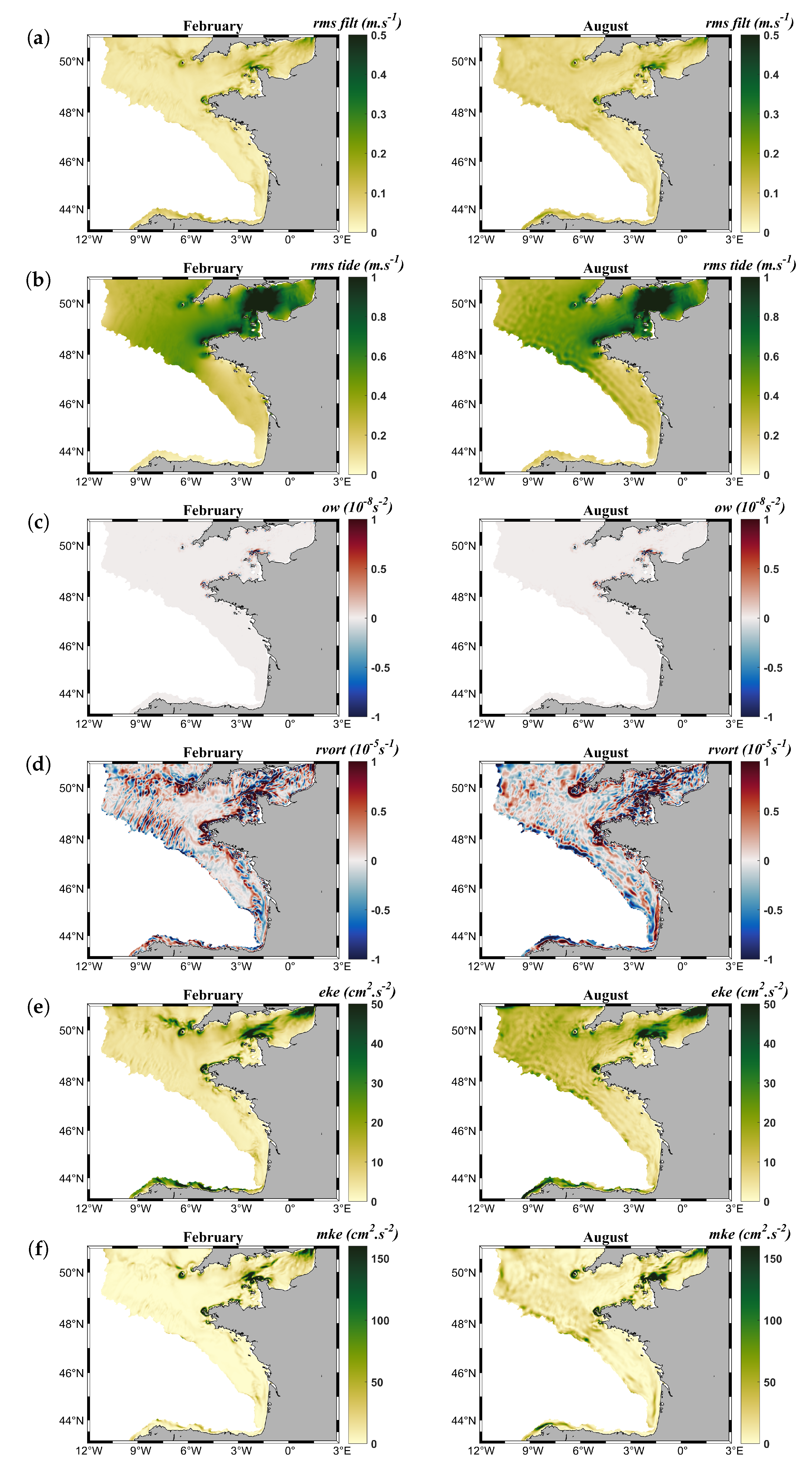
2.3. Model Outputs: EOVs and Derived Variables

Sea surface temperature, sea surface salinity, sea surface current velocities, sea surface elevation, along with three-dimensional temperature, salinity and density fields were extracted from the model at a one-hour time frequency. Based on these results, twelve variables among EOVs, and other sub-variables (hereinafter referred as subEOVs) of interest have been calculated (

Table 1. Essential ocean variables and sub-variables used and units.

EOV	Sub-EOV	Abr.	Units
Surface temperature		SST	°C
Surface salinity		SSS	PSU
Surface temperature and subsurface temperature	Mixed layer depth	MLD	m
	Deficit of potential energy	DPE	kg m−1 s−2
	SST gradient	GRADSST	°C m−1
	SSS gradient	GRADSSS	PSU m−1
Surface current	Root mean square of filtered current	RMS_FILT	m s−1
	Root mean square of tidal current	RMS_TIDE	m s−1
	Okubo–Weiss criterion	OW	s−2
	Relative vorticity	RVORT	s−2
	Eddy kinetic energy	EKE	m2 s−2
	Mean kinetic energy	MKE	m2 s−2

) using a monthly mean approach from January 2012 to December 2016, in order to detect large- and meso-scale physical processes in the regional area. The chosen hydrological and dynamical variables are well known to be of importance for the structuration of marine ecosystems [23,24,32]. Each variable is computed on a monthly basis. This choice is a compromise between the description of high-frequency variations and the computational cost of the statistical process described in Section 2.4.

Hydrological variables have been calculated as in [15]: Sea surface temperature (SST), sea surface salinity (SSS), mixed layer depth (MLD), deficit of potential energy (DPE), SST gradients (GRADSST) and SSS gradients (GRADSSS). SST is used to describe the seasonal cycle in variations of hydrological properties of water masses (Figure 2a). SSS allows to identify and to characterize the variability of river plumes, associated with low salinities (Figure 2b). MLD describes the thickness of the ocean layer exposed to atmospheric forcings. That corresponds to the pycnocline depth, calculated from three-dimensional density fields as the depth where the density increases by 0.03 kg·m⁻³ compared to a reference value taken at a 10-m depth [46]. If this criterion is not satisfied, the MLD is set to the maximum depth. Figure 2c shows the seasonality of the MLD from winter (left) to summer (right). DPE represents the amount of energy required to homogenize the water column and therefore characterizes the stratification intensity. It is calculated from [15,33]:

$$DPE=\frac{1}{H_0+\eta }{\int }_{-H_0}^{\eta }(\overline{\rho }-\rho )gzdz$$

(1)

where $\eta$ is the sea surface elevation, $H_0+\eta$ is the total water depth, $\rho$ is the water density, g is the acceleration of gravity equal to 9.81 m·s⁻² and $\overline{\rho }$ is the vertical mean water density.

Figure 2d shows the seasonal variations of DPE from winter (left), when the water column is weakly stratified and high values are mainly related to freshwater inputs associated to river plumes, to summer (right), when the stratification is strong except in coastal areas and in the English Channel area, mixed by strong tidal currents. The spatial distribution of the temperature and salinity tracers shows areas of small scale variations associated to frontal structures that delimit water masses with different hydrological properties [47,48,49]. These frontal structures can be detected using GRADSST and GRADSSS thanks to an arbitrary detection threshold (e.g., Figure 2e,f).

Dynamical variables related to physical mesoscale processes such as eddies [31,32,33] have been calculated: Root Mean Square (computed over one month) of low frequency currents filtered of the tidal component (RMS_FILT), Root Mean Square (computed over one month) of high frequency (tidal) currents (RMS_TIDE), Okubo–Weiss criterion (OW [50]), relative vorticity (RVORT), Eddy Kinetic Energy (EKE) and Mean Kinetic Energy (MKE). These dynamical variables have been calculated at a near-surface reference depth of 10 m rather than at the surface in order to avoid too high-frequency variations, due for example to the diurnal cycle and to accurately capture the turbulent activity and the baroclinic signature of the associated structures. RMS_FILT and RMS_TIDE were calculated using a Godin filtering method based on a weighted average of hourly-sampled data as in Simon [51] on each velocity component. An example of RMS_FILT and RMS_TIDE fields is given in Figure 3a,b, respectively. OW, RVORT, EKE and MKE were calculated from the zonal and meridional components of RMS_FILT. OW and RVORT were used to characterize vortex activities [50,52]. OW allows, thanks to the closed sign change contours, to detect the limits of vortex structures. The sign of RVORT is used to determine the nature of the vortex structure, cyclonic if it is positive and anticyclonic if it is negative. RVORT and OW are calculated as follows:

$$RVORT=\frac{\partial v}{\partial x}-\frac{\partial u}{\partial y},$$

(2)

$$OW={\left(\frac{\partial u}{\partial x}-\frac{\partial v}{\partial y}\right)}^2+{\left(\frac{\partial v}{\partial x}+\frac{\partial u}{\partial y}\right)}^2-RVOR{T}^2$$

(3)

where u and v are the zonal and meridian velocity components, respectively. An example of OW and RVORT fields is given in Figure 3c,d, respectively. MKE characterizes areas of strong current velocities and EKE is representative of the energy associated to turbulent activity. They are calculated following [31,32,33]:

$$EKE=\frac{1}{2}\left(\overline{{(u-\overline{u})}^2}+\overline{{(v-\overline{v})}^2}\right),$$

(4)

$$MKE=\frac{1}{2}\left({\overline{u}}^2+{\overline{v}}^2\right)$$

(5)

where $\overline{u}$ and $\overline{v}$ are the time-mean velocity components. An example of EKE and MKE is given in Figure 3e,f, respectively.

2.4. Statistical Analyses

2.4.1. Database

Each monthly mean physical field was calculated over an area of 471 × 720 points, corresponding to 339,120 points of which 97,678 points were land area and 151,162 points were beyond the 200 m isobath. The initial database was therefore made up of 339,120 points per time step × 12 physical variables × 60 months from January 2012 to December 2016, that being to $2.445\times {10}^8$ points.

2.4.2. Clustering Algorithm

In order to partition the abiotic component of the regional ecosystem, a preliminary statistical step consisted in a Principal Components Analysis (PCA) on scaled physical EOVs and subEOVs previously defined, for each month. PCA was used as a tool for dimensionality reduction, to reduce collinearity and to construct a composite unitless dataset, prior to the clustering analysis. Eigenvectors corresponding to 90% of the explained variance were selected to reduce the dimensionality of the data while minimizing the loss of information [53]. Partitioning was carried out using a hybrid two step clustering procedure using Hierarchical Agglomerative Clustering (HAC) and k-means. Hybrid approaches consist of the combination of different statistical methods in order to keep their individual advantages for a statistical protocol presenting certain constraints [54]. This two step procedure was chosen in order to (i) determine the number of clusters present at each month and (ii) find common clusters across months (Figure S1). In the first step of the partitioning process, spatial clusters were assessed on a monthly basis by Hierarchical Agglomerative Clustering (HAC) performed on selected eigenvectors from PCA on oceanographic variables and using Euclidean distance and Ward’s linkage [55]. HAC was chosen since its main advantage relies on its stability and because it does not require any a priori knowledge of number of groups. The optimal number of groups was determined using the Calinski-Harabasz criterion [56] within a range between 3 and 20, and over 500 iterations on the monthly dataset. As the HAC was carried out monthly, the clusters detected each month could not be reassigned to the following month. A second step has therefore been implemented to complete the regionalization process running k-means on the whole dataset (i.e., pluri-annual) to refine the monthly clusters labeling from HAC [57]. The optimal number of clusters was, for this “global clustering”, again determined using the Calinski-Harabasz clustering evaluation criterion, within a range of k potential clusters between the minimum and maximum number of clusters detected by HAC in the monthly step. This hybrid procedure resulted in a time series of monthly categorical maps composed by 10 clusters over 60 months (2012 to 2016), named “patch class” as defined by [58] (Figures S2 and S3).

All analyses of this section were performed using the “stat” package of the software R (V10) and MATLAB. Ocean circulation model hindcasts, subEOVs and HAC computation were performed using high-performance computing resources of DATARMOR infrastructure (http://www.ifremer.fr/pcdm).

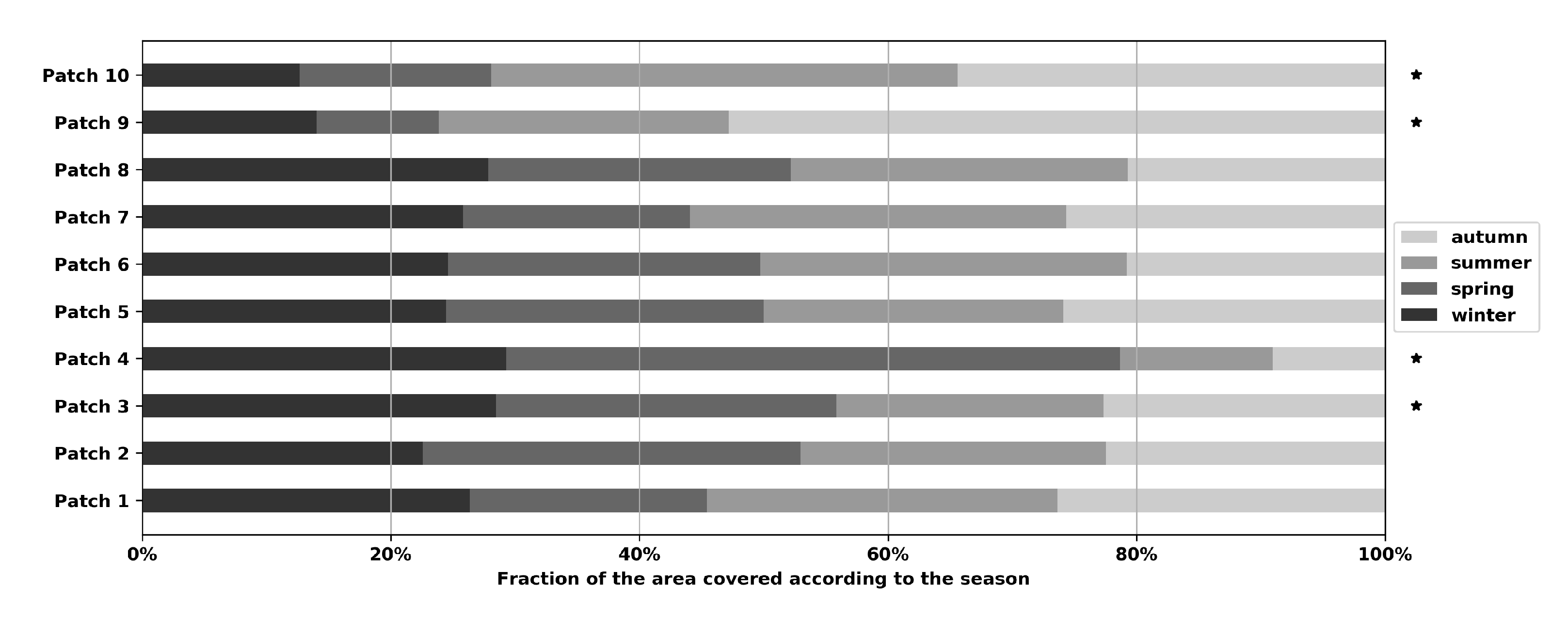
2.4.3. Patch Characterization

Generalized Boosted Regression Modeling (GBM) allows to build a nonlinear relationship between a response variable and explanatory variables. GBM maintains a monotonic relationship between the response (here, patch occurrence over 60 months) and each EOV and subEOV. GBM was used to characterize relative variable importance for each patch a posteriori. GBM models were chosen because Tree-based methods, such as RF or GBM, are more robust to collinearity [59]. Analyses were conducted on the 60-month average EOV climatologies for each patch. As patches were discriminated against the environmental variables, the object here was not to predict the patches with environmental variables, but to determine the most significant variables to characterize the groups. The GBM model calculates the relative influence of each variable in reducing the loss function [60]. We built models using the 75% training data to fit the GBM and the remainder 25% data were used to compute independent estimates of the loss function.

GBM models were constructed using the following parameters: The learning rate (lr) was equal to 0.01 to enhance the model’s performance [60]. The maximum nodes per tree were 5 to allow the predictor’s interactions. The bag fraction (the subsample fraction) was chosen in the medium range of 0.5, corresponding to the half of the training sample used to implement stochastic gradient descent to minimize overfitting. The relative variable importance, calculated by ranking the individual variables based on their relative importance, was computed using the default setting parameter as described in [61]. All analyses of this section were performed using the GBM package [60] of the software R (V10).

In addition, the categorization of variability for each EOV and subEOV was determined based on the 25th, 50th and 75th percentiles of the EOV and subEOVs distributions over the entire area and over the 60 months, and then compared to mean distributions of EOVs and subEOVs for each patch. Only the ranges of salinity variation were defined according to the following usual characteristics: PSU < 30, 30 < PSU < 34, 34 < PSU < 35 and PSU > 35 characterizing estuarine waters, ROFI (Region Of Freshwater Influence) waters, shelf waters and full salinity oceanic waters, respectively. The ranges of variation are relative to the study area and allow a typology of the characteristics of the water masses to be established in order to synthesize the information.

2.4.4. Seascape Unit Definition

The concept of seascape implies to take into account the combination of ecological and strategic considerations including administrative delimitations [62]. Seascapes units were designed by computing the spatial median of each patch relative to the frequency of detection of the patch over the time series (60 months). A seascape was defined as the combination of the administrative delimitation of the French marine subregions of the MSFD and the patch mosaic. The seascapes were therefore composed of sub-hydrographical patches simply referred to as “patches”. When a hydrological patch was split by administrative boundaries, it did not lose its physical properties and gained a new property linked to the marine sub-region to which it belongs. In addition, some contiguous patches may share boundaries with an existing part or overlap and their intersection as well as the mapping were conducted using the graphical information system QGIS.

3. Results

3.1. Pattern Analysis

The time series of the number of clusters detected by the HAC shows a range of variation between 8 and 13 clusters (Figure 4). The evaluation of the optimal number of clusters for the global k-means on the whole dataset gives an optimal number of clusters equal to ten (Figures S2 and S3). The ten patch classes are not systematically detected at each time step, indicating a spatio-temporal variability of the area partition illustrated in Figure 5, by the spatial occurrence of each group over the 60 months of the study (Figure S4).

Patch class 1 is distributed on the Bay of Biscay continental shelf, with a percentage of occurrence over 60 months between 10% and 80%, and a broad decreasing offshore-coastal gradient. The maximum stability is observed on the offshore part of the patch. Patch class 2 is a more coastal shelf patch, with a percentage of occurrence between 20% and 80%. A strong variability on the offshore part of the patch is observed, in contrast to Patch class 1. Patch class 3 is an oceanic group, located from the extreme northwest part of the study area to the entrance of the English Channel. This patch presents a strong disparity between the East and the West, reflecting a high variability in its eastern part over time and a very high stability in its western part with a percentage of occurrence over 60 months higher than 80%. Patch class 4 is close to the coast with a moderate percentage of occurrence, reflecting a relative variability in the area. Patch class 5, in the English Channel, shows a high stability in its central part, and variability in its periphery. Patch class 6 has a very small coastal extent and is highly stable along the period. Patch class 7, located just North of the whole area, has a spatial occurrence profile quite similar to Patch class 5, with high stability in the center of the cluster and a more variable periphery. Patch class 8 is located near the main rivers, with a high stability of detection occurrences. Patch class 9 represents the water masses along the Iberian coast, expressing non-recurring sub-patches along the French coast with a strong variability. Finally, Patch class 10 is located in the English Channel. It presents a fairly moderate percentage of occurrence over 60 months, probably related to its situation at the interface between Patch classes 3 and 5.

The analysis of patch classes area distributions according to the seasons reveals heterogeneity among groups (Figure 6). Patches classes 1, 2, 5, 6, 7 and 8 do not show significant differences in their seasonal area distributions, with a Kruskal-Wallis test p-value greater than 0.05 (not shown). Conversely, patch classes 3, 4, 9 and 10 present a strong heterogeneity in their ranges of area distributions according to the season, with a Kruskal-Wallis test p-value smaller than 0.05 (not shown). Patch class 3 is characterized by a larger distribution area during winter with a gradual decrease in spring and fall, and a minimal spatial extent in summer. Patch class 4 shows a larger extent in winter and spring, then a drastic reduction in summer and autumn. Patch class 9 is large in autumn, and much reduced in other seasons. Patch class 10 is characterized by large areas in summer and autumn, against smaller ones in winter and spring.

3.2. Hydrographical Patches Characteristics: Relating Statistical Patches with Abiotic Process

The relative importance of each derived variable, based on GBM model results, is shown in

Table 2. Rank of the individual variables based on their relative influence in each Generalized Boosted Regression Modeling (GBM) model. Dominant variables are written in bold.

EOVs	Patch 1	Patch 2	Patch 3	Patch 4	Patch 5	Patch 6	Patch 7	Patch 8	Patch 9	Patch 10
SST	3.7	1.3	20.3	2.9	3.7	2.7	1.5	0.3	2.2	3.6
SSS	5.5	5.1	0.2	49.3	1.4	2.1	3.8	55.9	2.0	11.6
MLD	10.3	65.3	0.5	0.9	5.9	4.1	0.4	0.4	4.9	11.7
DPE	54.5	2.9	40.3	3.6	5.1	1.1	0.8	0.2	1.9	28.9
GRADSST	7.9	9.1	33.2	1.0	2.3	1.8	0.3	0.1	1.4	1.3
GRADSSS	1.4	2.5	1.6	32.5	0.3	4.0	0.4	41.9	5.8	14.2
RMS_FILT	4.5	4.0	2.2	0.4	10.0	1.6	2.8	0.1	68.3	6.7
RMS_TIDE	4.5	3.4	0.4	7.4	52.8	2.2	1.3	0.4	1.3	16.5
OW	0.1	0.8	0.0	0.6	1.7	41.6	1.2	0.1	1.0	1.2
RVORT	0.1	0.8	0.1	0.5	3.2	17.0	0.4	0.3	0.7	0.6
EKE	5.3	0.8	0.9	0.5	8.6	4.3	86.1	0.1	1.8	1.3
MKE	2.1	4.0	0.3	0.4	5.0	17.5	1.0	0.1	8.7	2.4

. For information purposes, GBM evaluation and performance metrics are shown in Table S1. Ranges of categorization are defined in

Table 3. The 25th, 50th and 75th range of variability of EOVs distribution on the whole area, except for salinity, and associated typology.

EOV Name	≤25th	]25th;50th]	]50th;75th]	>75th
SST	≤11.4 cold	$]11.4;13.3]$ cool	$]13.3;15.9]$ moderate	>15.9 warm
SSS	≤30 estuarine waters	$]30;34]$ ROFI waters	$]34;35]$ shelf waters	>35 oceanic waters (full salinity)
MLD	≤7.6 unmixed	$]7.6;33]$ low mixed water	$]33;95.4]$ moderate mixed	>95.4 well mixed
DPE	≤0.7 unstratified	$]0.7;11.8]$ low stratified water	$]11.8;73.9]$ moderate stratified water	>73.9 well stratified water
log(GRADSST)	$\le -$11.6 no SST fronts	$]-11.6;-11.15]$ low SST front	$]-11.15;-10.5]$ moderate SST fronts	>−10.5 high SST fronts
log(GRADSSS)	$\le -$13.6 no SSS fronts	$]-14;-13.2]$ low SSS front	$]-12.9;-11.8]$ moderate SSS fronts	>−11.8 high SSS fronts
RMS_FILT	≤0.045 very low currents	$]0.045;0.06]$ low current	$]0.06;0.08]$ moderate current	>0.08 high current
RMS_TIDE	≤0.2 very low tidal flow	$]0.2;0.4]$ low tidal flow	$]0.4;0.5]$ moderate tidal flow	>0.5 high tidal flow
log(abs(RVORT))	$\le -$14 no vortex	$]-14;-13.2]$ low vortex	$]13.2;12.4]$ moderate vortex	>−12.4 high vortex
EKE	≤6.1 no turbulence	$]6.1;10.3]$ low turbulent water	$]10.3;18.7]$ moderate turbulent water	>18.7 highly turbulent water

. As the GBM model was computed using climatology over the 60 months, the model enables an average view of the dominant variables, but does not adequately represent individual months, or a seasonal signal. Combined with the seasonal analysis based on percentile ranges for each EOV and shown in

Table 4. Seasonal hydrographical typology of the 10 patch classes. Links between typology and the 25th, 50th, 75th range of variability of EOVs distribution are shown in Table 3.

Patch Number	Season	SST	SSS	MLD	DPE	GRADSST	GRADSSS	RMS_FILT	RMS_TIDE	RVORT	EKE
1	winter	moderate	oceanic	well mixed	moderate stratified	low	moderate	moderate	very low	low	moderate
1	spring	cool	oceanic	low mixed	moderate stratified	moderate	high	low	very low	low	moderate
1	summer	warm	shelf	unmixed	well stratified	high	high	low	very low	low	low
1	autumn	warm	oceanic	low mixed	well stratified	moderate	moderate	low	very low	low	moderate
2	winter	cold	shelf	well mixed	low stratified	high	high	moderate	low	moderate	moderate
2	spring	cold	shelf	low mixed	moderate stratified	high	high	low	low	moderate	moderate
2	summer	warm	shelf	low mixed	moderate stratified	high	high	low	low	moderate	low
2	autumn	warm	shelf	moderate mixed	moderate stratified	high	high	low	low	moderate	low
3	winter	cool	oceanic	well mixed	low stratified	low	low	moderate	moderate	low	moderate
3	spring	cold	oceanic	moderate mixed	low stratified	low	low	low	moderate	low	moderate
3	summer	warm	oceanic	unmixed	well stratified	low	low	low	low	low	low
3	autumn	moderate	oceanic	low mixed	well stratified	low	low	moderate	moderate	low	moderate
4	winter	cold	ROFI	low mixed	moderate stratified	high	high	low	very low	moderate	moderate
4	spring	cool	ROFI	low mixed	moderate stratified	high	high	very low	very low	low	low
4	summer	warm	ROFI	low mixed	moderate stratified	high	high	very low	very low	moderate	very low
4	autumn	moderate	ROFI	low mixed	moderate stratified	high	high	low	very low	moderate	low
5	winter	cold	oceanic	well mixed	unstratified	moderate	moderate	high	high	moderate	high
5	spring	cold	oceanic	well mixed	low stratified	low	moderate	high	high	high	high
5	summer	moderate	oceanic	moderate mixed	low stratified	moderate	low	high	high	moderate	high
5	autumn	moderate	oceanic	well mixed	low stratified	moderate	low	high	high	high	high
6	winter	cold	oceanic	well mixed	unstratified	moderate	low	high	high	high	high
6	spring	cold	oceanic	well mixed	low stratified	low	moderate	high	high	high	high
6	summer	moderate	oceanic	moderate mixed	low stratified	high	low	high	high	high	high
6	autumn	moderate	oceanic	well mixed	low stratified	moderate	low	high	high	high	high
7	winter	cold	oceanic	well mixed	low stratified	moderate	moderate	high	moderate	high	high
7	spring	cold	shelf	moderate mixed	low stratified	moderate	high	high	moderate	high	high
7	summer	moderate	shelf	low mixed	moderate stratified	high	high	high	high	high	high
7	autumn	moderate	shelf	moderate mixed	moderate stratified	moderate	moderate	high	high	high	high
8	winter	cold	estuary	low mixed	well stratified	high	high	low	very low	moderate	very low
8	spring	cold	estuary	low mixed	well stratified	high	high	very low	very low	moderate	very low
8	summer	warm	estuary	low mixed	moderate stratified	high	high	very low	low	moderate	very low
8	autumn	warm	estuary	moderate mixed	moderate stratified	high	high	very low	low	moderate	very low
9	winter	moderate	oceanic	moderate mixed	moderate stratified	moderate	moderate	high	very low	moderate	high
9	spring	moderate	oceanic	low mixed	moderate stratified	moderate	moderate	high	very low	moderate	high
9	summer	warm	oceanic	unmixed	well stratified	high	high	high	very low	high	high
9	autumn	warm	oceanic	low mixed	well stratified	high	high	high	very low	high	high
10	winter	cold	oceanic	well mixed	unstratified	moderate	low	moderate	high	moderate	moderate
10	spring	cold	oceanic	moderate mixed	low stratified	low	low	moderate	high	moderate	moderate
10	summer	moderate	oceanic	low mixed	moderate stratified	high	low	moderate	high	moderate	moderate
10	autumn	moderate	oceanic	moderate mixed	moderate stratified	moderate	low	moderate	high	moderate	moderate

, results allow the characterization of each patch class which is described below.

Patch class 1 is mainly characterized by DPE and MLD. It shows a seasonal signal, with shelf waters marked by salinity fronts and stratification in summer and autumn, against oceanic well-mixed waters with a lower frontal activity in winter. Spring corresponds to an intermediate situation, with moderately mixed waters. This patch is also characterized by low and moderate dynamical metrics, for example EKE, RMS_FILT and RMS_TIDE.

Patch class 2 is mainly driven by MLD but GRADSST also plays a non-negligible role. It can therefore be summarized as a group with well-mixed shelf waters in winter and moderately stratified waters in other seasons with a strong frontal activity throughout the year, influenced by fresh water outflows.

Patch class 3 is driven by a hydrological regime conducted by DPE, GRADSST and SST. However, the seasonal analysis reveals a strong variability with dominant mixed waters in winter and spring, while water masses are well-stratified in summer and autumn. It is an oceanic group, with a full salinity (>35 PSU).

Patch class 4 is mainly characterized by SSS and GRADSSS. SSS variability shows a strong relation with ROFI waters, with SSS values between 30 and 34 PSU. It is also characterized by an intense frontal activity with strong haline and thermal fronts, including a moderate stratification of the water body.

Patch class 5 is mainly characterized by RMS_TIDE and RMS_FILT. The seasonal analysis also highlights well-mixed water mass patterns due to strong currents, turbulence and tidal flows, but no significant seasonal signal is noticeable. The frontal activity is quite moderate throughout the year. It is an oceanic group with a full salinity.

Patch class 6 is mainly characterized by strong dynamical structures, with high values of OW, RVORT and MKE as relative key variables. The seasonal analysis confirms the GBM results on dynamical structures, and highlights that this patch is also influenced by residual currents and tidal flows, inducing fully mixed waters, without seasonal signal. It is an oceanic patch with a full salinity.

Patch class 7 is mainly driven by EKE corresponding to the mean flow coming from the Atlantic to the North Sea. The detailed analysis showed that it is also characterized by a seasonal signal with well mixed waters in winter and spring, against a relatively moderate stratification in summer and autumn, associated with strong tidal flows and residual currents with turbulent processes. This group is mainly a shelf water mass patch except in winter.

Patch class 8 is mainly characterized by the dominance of SSS and GRADSSS variables in the GBM model. This patch is an estuarine patch with reduced salinities and strong density gradients. The behavior of the patch does not show a seasonal signal.

Patch class 9 is mainly dominated by RMS_FILT. It corresponds to oceanic waters, with strong flows and frontal structures. It is also characterized by a seasonal signal, with a strong stratification associated with high frontal activity during summer and autumn against moderate stratification in winter and spring.

Patch class 10, unlike other patches, presents a certain heterogeneity with four relatively dominant variables: DPE, RMS_TIDE, GRADSSS, MLD and SSS, probably due to its position at the interface between Patch class 3 and Patch class 5 (Figure 5). The seasonal analysis shows a strong variability with strong and moderate mixed layer depths in winter and spring, and a strong frontal activity in summer unlike for other seasons.

3.3. Seascape Units

The coupling between water masses partitioning and the administrative delimitations of the MSFD French marine subregions is shown in Figure 7a. Each seascape is characterized by the proportion of each patch in the seascape and the area of each patch (

Table 5. Seascape composition metrics, patch proportion in the seascape and patch area.

Seascape	Patch	Patch Proportion	Patch Area (km2)
Bay of Biscay	S1 BB	0.53	42,691.8
Bay of Biscay	S2 BB	0.19	15,562.8
Bay of Biscay	S3 BB	0.17	13,270.2
Bay of Biscay	S4-1 BB	0.04	3230.7
Bay of Biscay	S4-2 BB	0.03	2726.7
Bay of Biscay	S4-3 BB	<0.01	283.0
Bay of Biscay	S5 BB	<0.01	67.1
Bay of Biscay	S6 BB	<0.01	17.9
Bay of Biscay	S8-1 BB	<0.01	259.0
Bay of Biscay	S8-2 BB	0.01	403.5
Bay of Biscay	S9 BB	0.01	728.7
Bay of Biscay	S10 BB	0.01	660.7
Celtic Seas	S2 CS	0.02	839.1
Celtic Seas	S3 CS	0.55	21,108.3
Celtic Seas	S5 CS	0.06	2460.4
Celtic Seas	S6 CS	0.01	438.2
Celtic Seas	S10 CS	0.36	13,801.6
English Channel–North Sea	S2 EC_NS	0.38	9170.0
English Channel–North Sea	S4 EC_NS	0.04	987.9
English Channel–North Sea	S5 EC_NS	0.26	6254.8
English Channel–North Sea	S6 EC_NS	0.02	404.1
English Channel–North Sea	S7 EC_NS	0.03	812.4
English Channel–North Sea	S8 EC_NS	<0.01	178.7
English Channel–North Sea	S10 EC_NS	0.27	6568.0

).

In the English Channel–Greater North Sea region, seven patches are identified. Patch 2 EC_NS is a shelf water patch counting for 19% of the total marine sub-region. Patches 4 EC_NS and 8 EC_NS are small patches representing less that 1% of the marine sub-region. Patch 6 EC_NS is a small patch covering 2% of the marine sub-region. Patch 7 EC_NS is exclusively found in this marine sub-region and corresponds to the channel between the North Sea and the English Channel, characterized by a small spatial extent (less than 5%). Patch 5 EC_NS is the third contributing patch in terms of spatial extent (26%). Finally Patch 10 corresponds to a surrounding background (27% of the total marine sub-region area).

In the Celtic seas region, five patches are identified. The region is spatially composed of two main patches, the patch 3 CS is related to the patch 3 detected previously with a spatial extent representing 55% of the total area and patch 10 CS (36%). The patch 2 CS corresponds to the patch class 2 but its spatial extent is much lower than in the other two marine sub-regions (2%). It is the same for patches 5 and 6 in this sub-region.

In the Bay of Biscay area, twelve patches are detected. Patch 1 BB is exclusively found in this marine sub-region and composes the main spatial part of the marine sub-region by occupying 53% of the area. Patch 2 BB is a shelf water mass group (19%). Patch 3 BB is the most southern part of patch 3 described previously counting for 17% of the marine sub-region area. In this subregion, Patch classes 4 and 8 are decomposed into 3 and 2 patches, respectively, according to the rivers influencing them. Thus, patches 4-1 BB, 4-2 BB and 4-3 BB are related to ROFI waters and patches 8-1 BB and 8-2 BB to estuaries. ROFI and estuarine patches represent a small fraction of the marine sub-region. Patches 5 BB, 6 BB and 10 BB are also present in this subregion, but their spatial extent is small (less than 2% of the total area). At least, patch 9 BB corresponds to a part of Iberian coastal waters into French waters, with a small proportion of the total area (1%).

Due to their spatial and temporal variability, some contiguous patches may share boundaries with an existing part or overlap. These overlapping areas are presented here as an interface between the patches (Figure 7b). The Celtic Sea shows a marked interface between patch 3 and 10, confirming the first results described previously. In the Eastern part of the English Channel and in the Bay of Biscay, main interfaces occur in transitional areas, between ROFI and shelf waters on one side and shelf water and oceanic waters on the other side. The Bay of Biscay is also characterized by an overlap between patch 3 BB and patch 1 BB.

4. Discussion

Seascape computation has required the implementation of added-value products from the OCO system: Calculation of EOVs and subEOVs and the classification of water masses patches. The input of the operational coastal oceanography has been crucial to this work. It indeed has enabled a procedure consistent with the international GOOS work [28], as well as the integration of data from CMEMS for some forcings and model validation [63] in order to build keystone steps for the implementation of MSFD-seascapes. The computation of several derived variables from OCO allowed us to synthesize the information provided by the state variables of the ocean circulation model. As such, they are a relevant tool to describe, for example, (i) stratification in the surface layers (mixed layer depth, intensity of stratification, etc.) from hydrological data, (ii) remarkable energy structures, such as frontal and eddy structures from current data (vorticity and Okubo–Weiss criterion). Our work is in line with previous literature such as [29,30,34], demonstrating that operational oceanography is a sufficiently mature and a major tool for the characterization of abiotic environmental conditions and providing high added-value products useful for marine management.

This work results in the development and the characterisation of a mosaic of dynamic hydrographic patches between 2012 and 2016 along the Atlantic coast of the French metropolitan EEZ. The hybrid combination of HAC and k-means allowed the construction of a time series of patch mosaics, resulting from a multivariate spatio-temporal partitioning. Each mosaic of the time series consists of a categorical map to define a picture of abiotic spatial units in the pelagic domain. From this time series, it was possible to define ten inter-annual main “patch classes” characterized by their spatio-temporal variability and hydrographical characteristics. Some are mainly dominated by hydrological processes such as the continental shelf Bay of Biscay patch class (number 1), the coastal shelf patch class (number 2), the Celtic Sea oceanic patch class (number 3), the river plume patch class (number 4) and the estuary patch class (number 8). Others are mainly dominated by hydrodynamical processes such as the tide-influenced patch class (number 5), the highly turbulent patch class (number 6), the high north flow patch class (number 7), and the coastal Iberian patch class (number 9). The transitional patch class (number 10) is the most variable one, probably reflecting its interface position. In addition, the analysis of the time series revealed differences in stability over time and space between patches, with stable patches (1,2,5,6,7,8) and less stable patches exhibiting significant seasonal variability (3,4,9 and 10).

In the context of the MSFD, specific sub-patches have been detected in each marine sub-region by combining the initial main patch classes with the MSFD regulatory delimitations. This combination corresponds to the definition of a “seascape” composed by sub-hydrographical patches and human consideration. Comparing our results to the literature, it appears that seascapes described and characterized here are consistent with previous works based on ocean partitioning, or works based on specific areas focusing on the processes involved. In the Eastern English Channel–North Sea French marine sub-region, our seascape is consistent with the one of [64], although the scope of the partitioning process and the choice of the derived variables were different. Their number of patches, within a range between seven and nine following the season, is quite similar to our results of seven detected water masses. Their classification showed some stable water masses comparable to the patches 8 EC_NS, 4 EC_NS, 5 EC_NS, 2 EC_NS and 10 EC_NS in the eastern part of the English Channel. They also detected patterns in the same geographical area as patch 7 EC_NS, but with a variability difficult to interpret. Patch 8 EC_NS corresponds to the Seine estuary and patch 4 EC_NS to its river plume. Patch 5 EC_NS is influenced by strong tidal currents in the Alderney Race area with the particularity to be the location of the strongest tidal currents in Europe. The shelf water patch 2 EC_NS corresponds to the coastal flow along the French coast generated by fluvial supplies as described by [65]. Patch 10 EC_NS is an oceanic transitional patch water. Patch 6 EC_NS, characterized by strong EKE and tidal currents, corresponds to many tide-induced gyres well described by [66].

The Celtic sea seascape is composed of five patches. Patch 3 CC in the western part is the biggest one, with a high seasonal dynamics. It reaches its maximum extension in winter. During spring, patch 10 CC enters the eastern part of patch 3. Since patch classes 10 and 3 are neighbours, and their spatial extent dynamics are inverted, it can be assumed that this corresponds to back and forth motion of the water mass from east to west depending on the season. This interface between patches 3 CC and 10 CC corresponds to the tide-induced Ushant frontal region. The Ushant front is set up at the end of spring. It is characterized by a stratified water mass offshore (patch 3 CC) and mixed waters near the coast (patch 10 CC) [67]. The presence of patches 5 CC and 6 CC, mainly dominated by tides and high turbulence is due to strong currents in the Fromveur Strait [68].

In the Bay of Biscay seascape, twelve patches are detected. Our results are consistent with those found by [15], but only for spring. The patch 3 BB corresponds to their group 8 “Northwestern shelf”, characterized by oceanic waters and thermal stratification in the springtime. The patch 1-BB is redundant with their patch 7 “Open shelf” along the continental slope, with oceanic waters and moderated stratification. Patch 2-BB corresponds to their patch 6 “Central shelf” characterized by shelf waters (34 PSU < SSS < 35 PSU) with the influence of outflow fresh water, moderate stratification, and low mixing flow during spring. For the other more coastal groups in the Bay of Biscay, the patterns are quite consistent, even if the number of groups differs. We find typical ROFI, patches 4-1 BB, 4-2 BB, 4-3 BB corresponding to groups 5, 4 and 3, respectively in [15], and estuarine water mass patterns 8-1 BB, 8-2 BB corresponding to group 2 in [15]. Patches 4-1BB and 8-1BB are related to the Loire river plume and estuary. Patches 4-2 BB and 8-2 BB correspond to the Gironde river plume and estuary. Patch 4-3 BB is related to the Adour river plume. Some patches present a strong seasonality in terms of spatial extent. For example, ROFI patches 4-1 and 4-2 BB are larger in winter and spring than in summer and autumn, which corresponds to the plumes of the Loire and the Gironde rivers analyzed in [69]. However, a difference can be noted concerning the period of maximum plume extension [69], using satellite turbidity data, showed that the maximum plume extension occurs in winter, whereas in our case it occurs in spring. It may be hypothesized that this difference could be due to the fact that [69] worked only on turbidity and that our study focuses on both hydrological and dynamical metrics, and also because the periods of study are different. It does suggest, however, the opportunity to integrate satellite turbidity data in a future work. Patches 5 BB, 6 BB and 10 BB are also present in this seascape, but are negligible compared to the global reach of the patch class. Patch class 9 on the Iberian coast corresponds to water masses along the continental slope bordering the Spanish coast. It is characterized by a strong seasonal signal with a maximum geographical extension in autumn, corresponding to water masses forming a tongue rising northwards at 2.5° W described by [70].

Our methodology has shown much strength to define seascape in the context of marine policy, but such partitioning methods have also some limitations, in particular on the detection of the patch class 9. The analysis of the global k-means (Figure S3) detects patch class 9 along the Spanish coast and in the Dover strait at the extreme north-east of the study area. However, it is unlikely to have system similarities between the Spanish coast and the Dover strait. By choosing to limit the study area to the 200m isobath, we included this very narrow zone along the Spanish coast. It appears, however, that this zone should not have been taken into account in the analyses, since it potentially generates a statistical bias, generating a statistical group that does not correspond to the oceanographic reality and is thus difficult to interpret. Furthermore, as shown in the ocean model description, low-frequency boundary conditions are provided by a large-scale ocean model. To prevent any inconsistency between boundary forcing and the interior computation domain, a sponge layer is located in the vicinity of the domain boundaries, where numerical solution is relaxed to boundary forcing. This numerical procedure is nevertheless likely to create artifacts near boundaries, and may lead to wrong patch detections. This may explain the pattern along the northern boundary in the oriental part of the English Channel and in the Celtic Sea. Several methodological improvements to the present work can thus be considered. The first one would be better defined boundaries of the study area, as previously stated. Another one would be to perform partitioning over smaller spatial extents, such as patches defined in this study, but this would raise questions about the balance between the need of a regional assessment and the relevant grain (spatial resolution) of the ocean circulation model. This indeed implies the use of high resolution coastal circulation models, and the need for observation networks adapted to their validation. On the French coasts, it is hoped that ILICO infrastructure [71] will enable significant progress on these issues, linked to operational oceanography in the coastal-nearshore domain.

The partitioning proposed here, points out the importance, for marine policies, to take into account not only hydrological variables related to stratification or temperature, but also dynamical ones related to oceanic currents, in order to better assess seascapes in the pelagic domain. Only based on abiotic characteristics, it allows to represent a specific level of the systems hierarchy, immediately above the ecosystem [72], as a counterpart of the benthic broad habitats described in the EUNIS classification. This strata is thus the abiotic part of the “ecomosaic” in the pelagic realm [72]. Furthermore, the development of a time series of seascapes categorial maps enables the use of usual landscape metrics to characterize seascapes in terms of composition and spatial configuration [58]. Ecologically speaking, this study provides a better understanding of the complexity of coastal-shelf areas in the french EEZ by highlighting the spatio-temporal variability of hydrographical patches. Indeed, seascapes variability induces moving boundaries between patches, i.e., interfaces that may be a proxy for marine ecotones, which are relevant places for ecological phenomenons such as nutrient injection, aggregation of matter, connectivity or trophic level elevation [3,14,24]. Thus, the assessment of a patch mosaic within seascape, based on hydrology and hydrography, could (i) help at defining areas of interest for human activities (e.g., strong current areas for marine renewable energy) and; (ii) allow the detection of, on the one hand, stable areas potentially hosting ecologically mature biocenosis, and, on the other hand, singular and dynamic patches, possibly associated with singular biological communities, which may require specific management measures. We therefore propose that detailed biological informations have to be integrated a posteriori, in a Russian doll’s logic, such as in the EUNIS classification, in order to assess finer strata of the hierarchical pelagic system. This would allow to assess the mosaic of biocenosis (small units) hosting in patches defined here (medium units) within the seascape (large units). This will be investigated in future works, in particular by integrating a posteriori satellite ocean color data or outputs from biogeochemical models.

5. Conclusions

The objective of this study was to compute and analyse a mosaic of abiotic patches in the coastal-shelf system of the french EEZ. The development process was carried out in a pluridisciplinary framework, integrating ocean modelling tools, statistical tools to compute partitioning and water mass characterization, in the context of marine policies. Along this framework, a precise set of specifications appeared to be relevant to implement: (i) It has to be based on hydrological and dynamical ocean variables calculated from outputs of a three-dimensional ocean circulation model such as HYCOM, (ii) partitioning the continental shelf area should take into account its dynamics over space and time and (iii) a hybrid partitioning process has to be computed. We therefore propose mosaics (seascapes), composed of standardised and understandable spatial units (patches) based on oceanic characteristics, and taking into account the combination of ecological and strategic considerations [62], such as marine spatial planning, including cross-border issues. Seascapes are a tool providing common synthetic environmental information which can enhance knowledge on the structure and architecture of ocean ecosystems, can better target marine monitoring on poorly known areas in order to better assess the state of water masses, and can give a setting for the development of operational indicators in the context of the MSFD.

References

1. Johnson, D.E.; Froján, C.B.; Turner, P.J.; Weaver, P.; Gunn, V.; Dunn, D.C.; Halpin, P.; Bax, N.J.; Dunstan, P.K. Reviewing the EBSA process: Improving on success. Mar. Policy 2018, 88, 75–85. [Google Scholar] [CrossRef]
2. Longhurst, A. Seasonal cycles of pelagic production and consumption. Prog. Oceanogr. 1995, 36, 77–167. [Google Scholar] [CrossRef]
3. Longhurst, A.R. Ecological Geography of the Sea; Elsevier: Amsterdam, The Netherlands, 2010. [Google Scholar]
4. Sherman, K.; Duda, A.M. Large marine ecosystems: An emerging paradigm for fishery sustainability. Fisheries 1999, 24, 15–26. [Google Scholar] [CrossRef]
5. Spalding, M.D.; Fox, H.E.; Allen, G.R.; Davidson, N.; Ferdaña, Z.A.; Finlayson, M.; Halpern, B.S.; Jorge, M.A.; Lombana, A.; Lourie, S.A.; et al. Marine ecoregions of the world: A bioregionalization of coastal and shelf areas. BioScience 2007, 57, 573–583. [Google Scholar] [CrossRef] [Green Version]
6. Spalding, M.D.; Agostini, V.N.; Rice, J.; Grant, S.M. Pelagic provinces of the world: A biogeographic classification of the world’s surface pelagic waters. Ocean. Coast. Manag. 2012, 60, 19–30. [Google Scholar] [CrossRef]
7. Witze, A. Ocean ecosystems mapped in unprecedented 3D detail. Nature 2017, 541, 10–11. [Google Scholar] [CrossRef] [Green Version]
8. Pauly, D.; Christensen, V.; Froese, R.; Longhurst, A.; Platt, T.; Sathyendranath, S.; Sherman, K.; Watson, R. Mapping fisheries onto marine ecosystems: A proposal for a consensus approach for regional, oceanic and global integrations. Fish. Cent. Res. Rep. 2000, 8, 13–22. [Google Scholar]
9. Reygondeau, G.; Dunn, D. Pelagic Biogeography. Encycl. Ocean. Sci. 2018, 588, 598. [Google Scholar]
10. Nieblas, A.E.; Drushka, K.; Reygondeau, G.; Rossi, V.; Demarcq, H.; Dubroca, L.; Bonhommeau, S. Defining Mediterranean and Black Sea biogeochemical subprovinces and synthetic ocean indicators using mesoscale oceanographic features. PLoS ONE 2014, 9, e111251. [Google Scholar] [CrossRef] [Green Version]
11. Reygondeau, G.; Guieu, C.; Benedetti, F.; Irisson, J.O.; Ayata, S.D.; Gasparini, S.; Koubbi, P. Biogeochemical regions of the Mediterranean Sea: An objective multidimensional and multivariate environmental approach. Prog. Oceanogr. 2017, 151, 138–148. [Google Scholar] [CrossRef] [Green Version]
12. Ayata, S.D.; Irisson, J.O.; Aubert, A.; Berline, L.; Dutay, J.C.; Mayot, N.; Nieblas, A.E.; d’Ortenzio, F.; Palmiéri, J.; Reygondeau, G.; et al. Regionalisation of the Mediterranean basin, a MERMEX synthesis. Prog. Oceanogr. 2018, 163, 7–20. [Google Scholar] [CrossRef] [Green Version]
13. Steele, J.H. The ocean ‘landscape’. Landsc. Ecol. 1989, 3, 185–192. [Google Scholar] [CrossRef]
14. Pittman, S.J. Seascape Ecology; John Wiley & Sons: Hoboken, NJ, USA, 2017. [Google Scholar]
15. Planque, B.; Lazure, P.; Jégou, A.M. Detecting hydrological landscapes over the Bay of Biscay continental shelf in spring. Clim. Res. 2004, 28, 41–52. [Google Scholar] [CrossRef] [Green Version]
16. Planque, B.; Lazure, P.; Jegou, A.M. Typology of hydrological structures modelled and observed over the Bay of Biscay shelf. Sci. Mar. 2006, 70, 43–50. [Google Scholar] [CrossRef] [Green Version]
17. Oliver, M.J.; Glenn, S.; Kohut, J.T.; Irwin, A.J.; Schofield, O.M.; Moline, M.A.; Bissett, W.P. Bioinformatic approaches for objective detection of water masses on continental shelves. J. Geophys. Res. Ocean. 2004, 109. [Google Scholar] [CrossRef]
18. Davies, C.E.; Moss, D.; Hill, M.O. EUNIS habitat classification revised 2004. In Report to: European Environment Agency-European Topic Centre on Nature Protection and Biodiversity; EEA Glossary: Copenhagen, Denmark, 2004; pp. 127–143. [Google Scholar]
19. Madden, C.; Goodin, K.; Allee, R.; Cicchetti, G.; Moses, C.; Finkbeiner, M.; Bamford, D. Coastal and Marine Ecological Classification Standard; NOAA and Nature Serv: Arlington, Virginia, 2009. [Google Scholar]
20. Ferry-Graham, L.A.; Bolnick, D.I.; Wainwright, P.C. Using functional morphology to examine the ecology and evolution of specialization. Integr. Comp. Biol. 2002, 42, 265–277. [Google Scholar] [CrossRef]
21. Zobel, M. The relative of species pools in determining plant species richness: An alternative explanation of species coexistence? Trends Ecol. Evol. 1997, 12, 266–269. [Google Scholar] [CrossRef]
22. Kai, E.T.; Rossi, V.; Sudre, J.; Weimerskirch, H.; Lopez, C.; Hernandez-Garcia, E.; Marsac, F.; Garçon, V. Top marine predators track Lagrangian coherent structures. Proc. Natl. Acad. Sci. USA 2009, 106, 8245–8250. [Google Scholar]
23. Scales, K.L.; Miller, P.I.; Hawkes, L.A.; Ingram, S.N.; Sims, D.W.; Votier, S.C. On the front line: Frontal zones as priority at-sea conservation areas for mobile marine vertebrates. J. Appl. Ecol. 2014, 51, 1575–1583. [Google Scholar] [CrossRef] [Green Version]
24. Bakun, A. Patterns in the ocean: Ocean processes and marine population dynamics. Oceanogr. Lit. Rev. 1997, 5, 530. [Google Scholar]
25. Bojinski, S.; Verstraete, M.; Peterson, T.C.; Richter, C.; Simmons, A.; Zemp, M. The concept of essential climate variables in support of climate research, applications, and policy. Bull. Am. Meteorol. Soc. 2014, 95, 1431–1443. [Google Scholar] [CrossRef]
26. Miloslavich, P.; Bax, N.J.; Simmons, S.E.; Klein, E.; Appeltans, W.; Aburto-Oropeza, O.; Andersen Garcia, M.; Batten, S.D.; Benedetti-Cecchi, L.; Checkley, D.M., Jr.; et al. Essential ocean variables for global sustained observations of biodiversity and ecosystem changes. Glob. Chang. Biol. 2018, 24, 2416–2433. [Google Scholar] [CrossRef] [PubMed]
27. Reyers, B.; Stafford-Smith, M.; Erb, K.H.; Scholes, R.J.; Selomane, O. Essential variables help to focus sustainable development goals monitoring. Curr. Opin. Environ. Sustain. 2017, 26, 97–105. [Google Scholar] [CrossRef]
28. Bax, N.J.; Appeltans, W.; Brainard, R.; Duffy, J.E.; Dunstan, P.; Hanich, Q.; Harden Davies, H.; Hills, J.; Miloslavich, P.; Muller-Karger, F.E.; et al. Linking capacity development to GOOS monitoring networks to achieve sustained ocean observation. Front. Mar. Sci. 2018, 5, 346. [Google Scholar] [CrossRef]
29. Rinaldi, E.; Orasi, A.; Morucci, S.; Colella, S.; Inghilesi, R.; Bignami, F.; Santoleri, R. How can operational oceanography products contribute to the European Marine Strategy Framework Directive? The Italian case. J. Oper. Oceanogr. 2016, 9, s18–s32. [Google Scholar] [CrossRef]
30. Fratianni, C.; Pinardi, N.; Lalli, F.; Simoncelli, S.; Coppini, G.; Pesarino, V.; Bruschi, A.; Cassese, M.; Drudi, M. Operational oceanography for the Marine Strategy Framework Directive: The case of the mixing indicator. J. Oper. Oceanogr. 2016, 9, s223–s233. [Google Scholar] [CrossRef]
31. Testor, P.; Gascard, J.C. Large scale flow separation and mesoscale eddy formation in the Algerian Basin. Prog. Oceanogr. 2005, 66, 211–230. [Google Scholar] [CrossRef]
32. Tew-Kai, E.; Marsac, F. Patterns of variability of sea surface chlorophyll in the Mozambique Channel: A quantitative approach. J. Mar. Syst. 2009, 77, 77–88. [Google Scholar] [CrossRef]
33. Huret, M.; Sourisseau, M.; Petitgas, P.; Struski, C.; Léger, F.; Lazure, P. A multi-decadal hindcast of a physical–biogeochemical model and derived oceanographic indices in the Bay of Biscay. J. Mar. Syst. 2013, 109, S77–S94. [Google Scholar] [CrossRef] [Green Version]
34. She, J.; Allen, I.; Buch, E.; Crise, A.; Johannessen, J.A.; Le Traon, P.Y.; Lips, U.; Nolan, G.; Pinardi, N.; Reißmann, J.H.; et al. Developing European operational oceanography for Blue Growth, climate change adaptation and mitigation, and ecosystem-based management. Ocean. Sci. 2016, 12, 953–976. [Google Scholar] [CrossRef] [Green Version]
35. Bleck, R. An oceanic general circulation model framed in hybrid isopycnic-Cartesian coordinates. Ocean. Model. 2002, 4, 55–88. [Google Scholar] [CrossRef]
36. Pichon, A.; Morel, Y.; Baraille, R.; Quaresma, L. Internal tide interactions in the Bay of Biscay: Observations and modelling. J. Mar. Syst. 2013, 109, S26–S44. [Google Scholar] [CrossRef]
37. Quaresma, L.S.; Pichon, A. Modelling the barotropic tide along the West-Iberian margin. J. Mar. Syst. 2013, 109, S3–S25. [Google Scholar] [CrossRef]
38. Morel, Y.; Baraille, R.; Pichon, A. Time splitting and linear stability of the slow part of the barotropic component. Ocean. Model. 2008, 23, 73–81. [Google Scholar] [CrossRef]
39. Lahaye, S.; Gouillon, F.; Baraille, R.; Pichon, A.; Pineau-Guillou, L.; Morel, Y. A numerical scheme for modeling tidal wetting and drying. J. Geophys. Res. Ocean. 2011, 116. [Google Scholar] [CrossRef] [Green Version]
40. Jourdan, D.; Paradis, D.; Pasquet, A.; Michaud, H.; Gouillon, F.; Baraille, R.; Biscara, L.; Voineson, G.; Ohl, P. Le projet HOMONIM. In Proceedings of the Comite Scientifique Scientific Committee, Brest, France, 3–4 July 2014; p. 88. [Google Scholar]
41. Lellouche, J.M.; Greiner, E.; Le Galloudec, O.; Garric, G.; Regnier, C.; Drevillon, M.; Benkiran, M.; Testut, C.E.; Bourdalle-Badie, R.; Gasparin, F.; et al. Recent updates to the Copernicus Marine Service global ocean monitoring and forecasting real-time 1/ 12° high-resolution system. Ocean. Sci. 2018, 14, 1093–1126. [Google Scholar] [CrossRef] [Green Version]
42. Carrère, L.; Lyard, F. Modeling the barotropic response of the global ocean to atmospheric wind and pressure forcing-comparisons with observations. Geophys. Res. Lett. 2003, 30. [Google Scholar] [CrossRef] [Green Version]
43. Large, W.G.; McWilliams, J.C.; Doney, S.C. Oceanic vertical mixing: A review and a model with a nonlocal boundary layer parameterization. Rev. Geophys. 1994, 32, 363–403. [Google Scholar] [CrossRef] [Green Version]
44. Descamps, L.; Labadie, C.; Joly, A.; Bazile, E.; Arbogast, P.; Cébron, P. PEARP, the Météo-France short-range ensemble prediction system. Q. J. R. Meteorol. Soc. 2015, 141, 1671–1685. [Google Scholar] [CrossRef]
45. Fichaut, M.; Bonnat, A.; Carval, T.; Lecornu, F.; Le Roux, J.; Moussat, E.; Nonnotte, L.; Tarot, S. Data Centre for French Coastal Operational Oceanography. Mediterr. Mar. Sci. 2011, 12, 70–79. [Google Scholar] [CrossRef]
46. de Boyer Montégut, C.; Madec, G.; Fischer, A.S.; Lazar, A.; Iudicone, D. Mixed layer depth over the global ocean: An examination of profile data and a profile-based climatology. J. Geophys. Res. Ocean. 2004, 109. [Google Scholar] [CrossRef]
47. Woodson, C.; McManus, M.; Tyburczy, J.; Barth, J.; Washburn, L.; Caselle, J.; Carr, M.; Malone, D.; Raimondi, P.; Menge, B.; et al. Coastal fronts set recruitment and connectivity patterns across multiple taxa. Limnol. Oceanogr. 2012, 57, 582–596. [Google Scholar] [CrossRef] [Green Version]
48. Woodson, C.B.; Litvin, S.Y. Ocean fronts drive marine fishery production and biogeochemical cycling. Proc. Natl. Acad. Sci. USA 2015, 112, 1710–1715. [Google Scholar] [CrossRef] [Green Version]
49. Acha, E.M.; Piola, A.; Iribarne, O.; Mianzan, H. Ecological Processes at Marine Fronts: Oases in the Ocean; Springer: Berlin/Heidelberg, Germany, 2015. [Google Scholar]
50. Okubo, A. Horizontal dispersion of floatable particles in the vicinity of velocity singularities such as convergences. In Deep Sea Research and Oceanographic Abstracts; Elsevier: Amsterdam, The Netherlands, 1970; Volume 17, pp. 445–454. [Google Scholar]
51. Simon, B.; Gonella, J. La Marée Océanique Côtière; Institut Océanographique: Paris, France, 2007. [Google Scholar]
52. Weiss, J. The dynamics of enstrophy transfer in two-dimensional hydrodynamics. Phys. D Nonlinear Phenom. 1991, 48, 273–294. [Google Scholar] [CrossRef]
53. Smith, L. A tutorial on principal component analysis. In Elementary Linear Algebra 5e; John Wiley Sons: Hoboken, NJ, USA, 2002; Volume 2012. [Google Scholar]
54. Sun, T.; Shu, C.; Li, F.; Yu, H.; Ma, L.; Fang, Y. An efficient hierarchical clustering method for large datasets with map-reduce. In Proceedings of the 2009 International Conference on Parallel and Distributed Computing, Applications and Technologies, Boston, MA, USA, 24–26 September 2009; pp. 494–499. [Google Scholar]
55. Ward, J.H., Jr. Hierarchical grouping to optimize an objective function. J. Am. Stat. Assoc. 1963, 58, 236–244. [Google Scholar] [CrossRef]
56. Caliński, T.; Harabasz, J. A dendrite method for cluster analysis. Commun. Stat. Theory Methods 1974, 3, 1–27. [Google Scholar] [CrossRef]
57. Huquet, B.; Leclerc, H.; Ducrocq, V. Characterization of French dairy farm environments from herd-test-day profiles. J. Dairy Sci. 2012, 95, 4085–4098. [Google Scholar] [CrossRef] [Green Version]
58. McGarigal, K. Landscape pattern metrics. Wiley Statsref Stat. Ref. Online 2014. [Google Scholar]
59. Dormann, C.F.; Elith, J.; Bacher, S.; Buchmann, C.; Carl, G.; Carré, G.; Marquéz, J.R.G.; Gruber, B.; Lafourcade, B.; Leitão, P.J.; et al. Collinearity: A review of methods to deal with it and a simulation study evaluating their performance. Ecography 2013, 36, 27–46. [Google Scholar] [CrossRef]
60. Ridgeway, G.; Boehmke, B. Generalized Boosted Regression Models; Jay. gbm, 2.1.5; Brandon Greenwell: Cincinnati, OH, USA, 2019. [Google Scholar]
61. Friedman, J.H. Greedy function approximation: A gradient boosting machine. Ann. Stat. 2001, 1189–1232. [Google Scholar] [CrossRef]
62. Atkinson, S.; Esters, N.; Farmer, G.; Lawrence, K.; McGilvray, F. The Seascapes Guidebook: How to Select, Develop and Implement Seascapes; Conservation International: Arlington, VA, USA, 2011. [Google Scholar]
63. Szekely, T.; Gourrion, J.; Pouliquen, S.; Reverdin, G. The CORA 5.2 dataset for global in situ temperature and salinity measurements: Data description and validation. Ocean. Sci. 2019, 15, 1601–1614. [Google Scholar] [CrossRef] [Green Version]
64. Delavenne, J.; Marchal, P.; Vaz, S. Defining a pelagic typology of the eastern English Channel. Cont. Shelf Res. 2013, 52, 87–96. [Google Scholar] [CrossRef] [Green Version]
65. Brylinski, J.; Lagadeuc, Y.; Gentilhomme, V.; Dupont, J.; Lafite, R.; Dupeuble, P.; Huault, M.; Auger, Y. Le fleuve côtier: Un phénomène hydrologique important en Manche Orientale. Exemple du Pas-de-Calais. Oceanol. Acta Spec. Issue 1991, 11, 197–203. [Google Scholar]
66. Salomon, J.C.; Breton, M. An atlas of long-term currents in the Channel. Oceanol. Acta 1993, 16, 439–448. [Google Scholar]
67. Yelekçi, Ö.; Charria, G.; Capet, X.; Reverdin, G.; Sudre, J.; Yahia, H. Spatial and seasonal distributions of frontal activity over the French continental shelf in the Bay of Biscay. Cont. Shelf Res. 2017, 144, 65–79. [Google Scholar] [CrossRef] [Green Version]
68. Thiébaut, M.; Sentchev, A. Estimation of tidal stream potential in the Iroise Sea from velocity observations by high frequency radars. Energy Procedia 2015, 76, 17–26. [Google Scholar] [CrossRef] [Green Version]
69. Costoya, X.; Fernández-Nóvoa, D.; Decastro, M.; Santos, F.; Lazure, P.; Gómez-Gesteira, M. Modulation of sea surface temperature warming in the B ay of B iscay by L oire and G ironde R ivers. J. Geophys. Res. Ocean. 2016, 121, 966–979. [Google Scholar] [CrossRef] [Green Version]
70. Friocourt, Y.; Levier, B.; Speich, S.; Blanke, B.; Drijfhout, S. A regional numerical ocean model of the circulation in the Bay of Biscay. J. Geophys. Res. Ocean. 2007, 112. [Google Scholar] [CrossRef] [Green Version]
71. Cocquempot, L.; Delacourt, C.; Paillet, J.; Riou, P.; Aucan, J.; Castelle, B.; Charria, G.; Claudet, J.; Conan, P.; Coppola, L.; et al. Coastal ocean and nearshore observation: A French case study. Front. Mar. Sci. 2019, 6, 324. [Google Scholar] [CrossRef] [Green Version]
72. Peano, A.; Cassatella, C. Landscape assessment and monitoring. In Landscape Indicators; Springer: Berlin/Heidelberg, Germany, 2011; pp. 1–14. [Google Scholar]
Figure 1. Map of the study area showing the bathymetry and French Marine Strategy Framework Directive (MSFD, Directive 2008/56/CE) sub-marine regions: Bay of Biscay (white line), East English Channel–North Sea (black dashed line), Celtic Seas (black dot-dashed line).
Jmse 08 00585 g001
Figure 2. Illustration of monthly hydrological Essential Ocean Variables (EOVs) in February (left) and August (right): (a) Sea surface temperature (SST), (b) sea surface salinity (SSS), (c) mixed layer depth (MLD), (d) deficit of potential energy (DPE), (e) SST gradients (GRADSST) and (f) SSS gradients (GRADSSS).
Jmse 08 00585 g002
Figure 3. Illustration of monthly dynamical EOVs in February (left) and August (right): (a) Root Mean Square (computed over one month) of low frequency currents filtered of the tidal component (RMS_FILT), (b) Root Mean Square (computed over one month) of high frequency (tidal) currents (RMS_TIDE), (c) Okubo–Weiss criterion (OW), (d) relative vorticity (RVORT), (e) Eddy Kinetic Energy (EKE) and (f) Mean Kinetic Energy (MKE).
Jmse 08 00585 g003
Figure 4. Distribution of the number of clusters detected by Hierarchical Agglomerative Clustering (HAC).
Jmse 08 00585 g004
Figure 5. Spatial occurrence of the ten hydrographical patches over the 60 month experiment.
Jmse 08 00585 g005
Figure 6. Geographical extent proportion (percents of pixels) of the 10 hydrodynamical patch classes, following the season. Asterisks show patch class with a significant spatial extent variation according to season.
Jmse 08 00585 g006
Figure 7. (a) Seascapes resulting in the overlap between hydrographical patches and MSFD marine sub-regions. The nomenclature of the patch name reveals its hydrographic specificities by the patch number (e.g., 2) and its administrative affiliation: EC-NS (English Channel–North Sea), CS (Celtic Seas) and BB (Bay of Biscay) and (b) interface between median patches.
Jmse 08 00585 g007