Study on the Capacity of an Active Phase Controller for Autonomous Grid Connection

Abstract

For the efficient power allocation of the distribution line, several studies on intelligent distribution management systems that enable connection or separation between distribution networks are being conducted. However, in case the systems are linked together and if the voltage and phase of each distribution network are different, uncontrolled circulating current and inrush current flow into the line. To resolve this, we introduced the active phase controller (APC) as a solution and performed an analysis using the capacity calculation method for the APC connected to each distribution network. When connecting lines between distribution networks, the phase of each contact was ensured to be the same. Specifically, the phase value compensated by each APC is different because the amounts of active power and reactive power to be controlled are also different. In this study, we analyzed the APC capacity according to the impedance state of the distribution line and calculated the APC output voltage for the phase matching of each distribution network at the connection point. As a result, the minimum design capacity of APC was derived; moreover, simulation results were used to validate the analysis.

1. Introduction

When distributed generators are connected to distribution lines, their response to variations in the line characteristics is weak [1,2,3,4,5]. Therefore, as the number of renewable energy sources, the amount of power transmitted from the transmission network to the distribution network decreases, which further leads to the frequent occurrence of the reversed power flow phenomenon, i.e., the amount of power transmitted from the distribution network to the transmission network increases [6,7,8]. Therefore, the substation capacities of existing distribution networks are designed considering higher margins, such as an increased demand power of the line and an exceeded maximum allowable capacity, for continuous operation in various unfavorable conditions. However, designing substation capacities with higher margins generates not only a disproportionate design cost but also issues such as decreased utilization factor and degraded overall efficiency. In addition, although substation is designed considering a higher margin, the protection co-ordination problem occurs due to local line capacity violation and reversed power flow on the substation caused by the load variations [9,10,11,12,13,14]. To resolve this, passive problem-solving methods, such as securing an allowable capacity by adding substations, are proposed. Therefore, without excessive capacity expansion according to the rapidly changing load, the active-type problem-solving method through the autonomous reconfiguration of the line is reviewed. The implementation of such a method can reduce the burden on the line and increase the utilization factor through mutual coordination with a nearby distribution line with sufficient capacity.

The autonomous reconfiguration of the distribution system should be able to directly change the loop or mesh shape of the system.

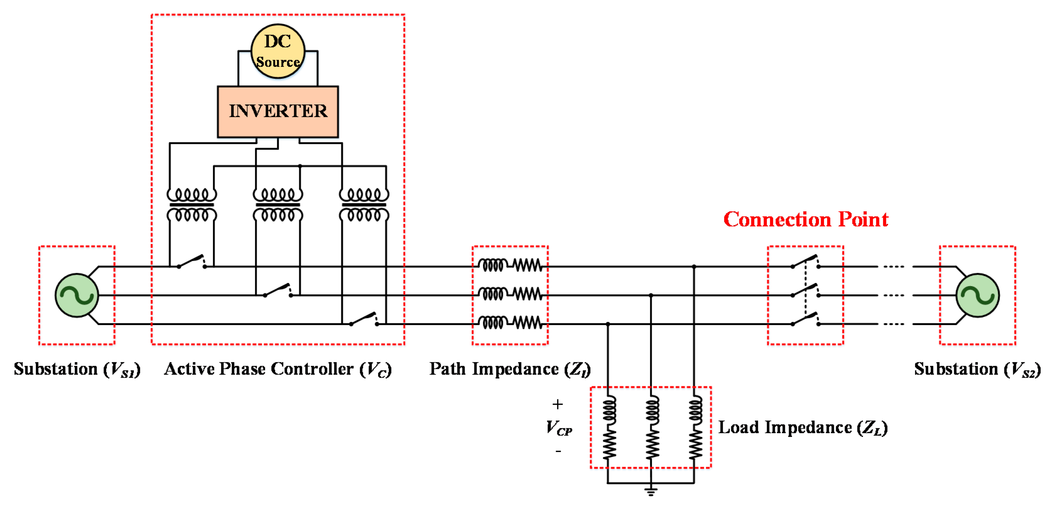
In addition, the distribution network may be arbitrarily connected or separated to ensure optimum power supply to each line [15,16,17,18,19]. However, uncontrolled circulating current and inrush current are generated in the line when the voltage and phase between the lines are different from each other at the connection point (CP). If an overcurrent flows into the line in this way, the peripheral circuit breaker malfunctions, which can result in unexpected power outage. Therefore, a method for matching the voltages and phases at the connection point is necessary. In this paper, we introduced an active phase controller (APC) for the autonomous reconfiguration of lines based on the 6-switch inverter. As shown in Figure 1, the APC is connected in series behind the substation. Furthermore, it controls the phase of the connection point through generation of a voltage drop by inserting serial compensation voltage (V_C) into line. Moreover, the magnitudes of the active power and reactive power output to the APC vary based on the load impedance and the adjusted phase [20,21,22,23,24,25]. Considering this, analysis was performed based on various APC installation scenarios, and the optimal connection point voltage of the APC was calculated using the formulas provided herein to enable efficient control.

2. Theoretical Analysis

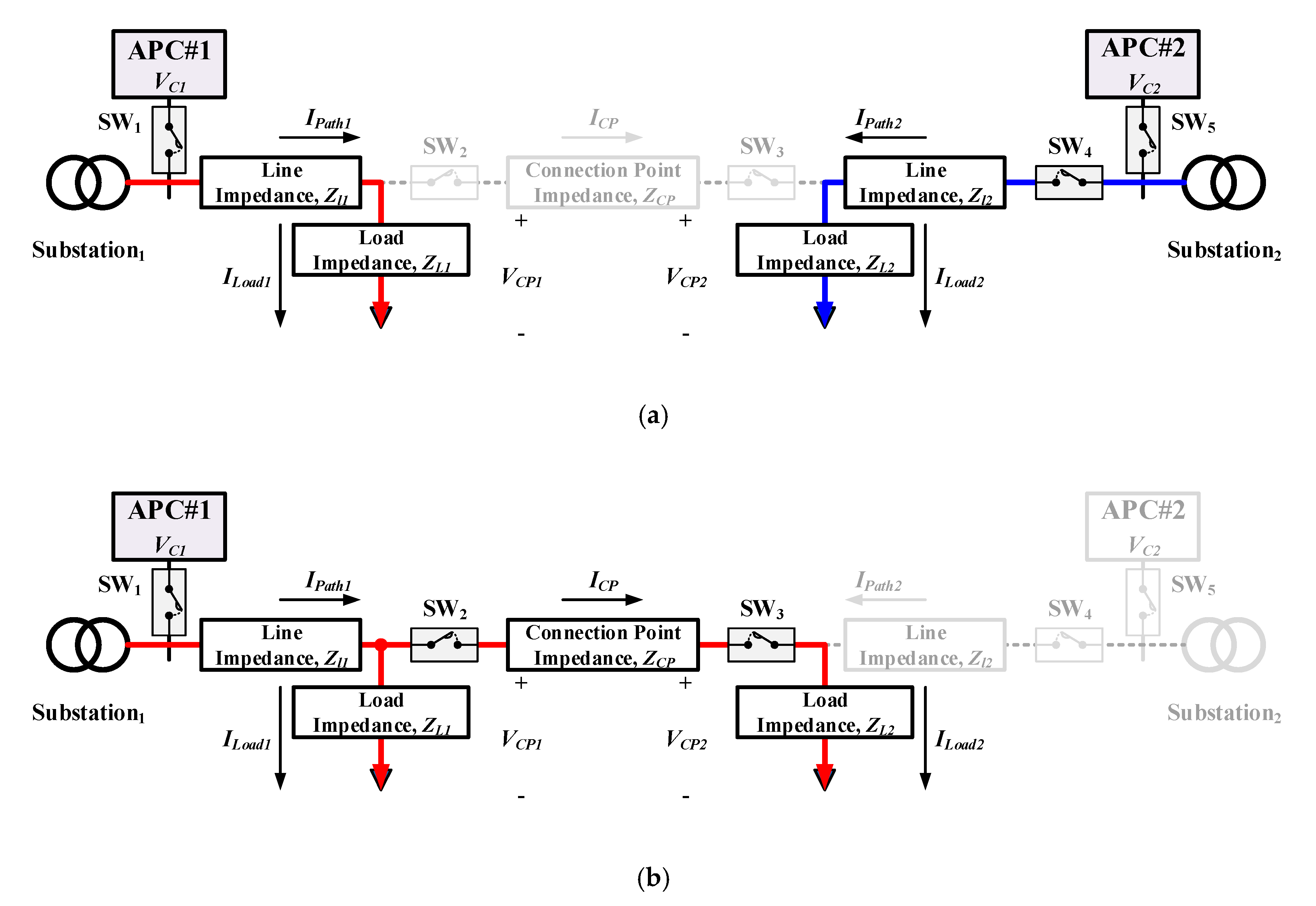
Figure 2a depicts the situation before autonomic reconfiguration between the lines. Normally, load impedance#1 and load impedance#2 receive power from substation#1 and substation#2, respectively. At this time, if a problem such as increased demand power or exceeded maximum allowable capacity occurs in substation#2, the problem is alleviated through autonomic reconfiguration between the lines, as shown in Figure 2b. However, uncontrolled circulating current and inrush current are generated in the line when the voltage and phase between the lines are different at the connection point. Owing to this difference, if an overcurrent flows into the line, the peripheral circuit breaker malfunctions, which may cause an unexpected power outage. To resolve this, an APC is installed behind each substation. Specifically, the APC is installed in series with the substation (V_S) to apply a serial compensation voltage to the line, and the voltage between the connection points is matched using a voltage drop. As a result, the magnitude and phase of the voltage at the connection point are equal to those of the voltage applied to the load impedance. The actual magnitude and phase of the voltage at the connection point were measured through a phasor measurement unit (PMU). In addition, the line impedance exists in series with the substation, whereas the load impedance exists in parallel. Furthermore, if line expansion and load fluctuation are neglected, each impedance and power factor could be treated as a constant.

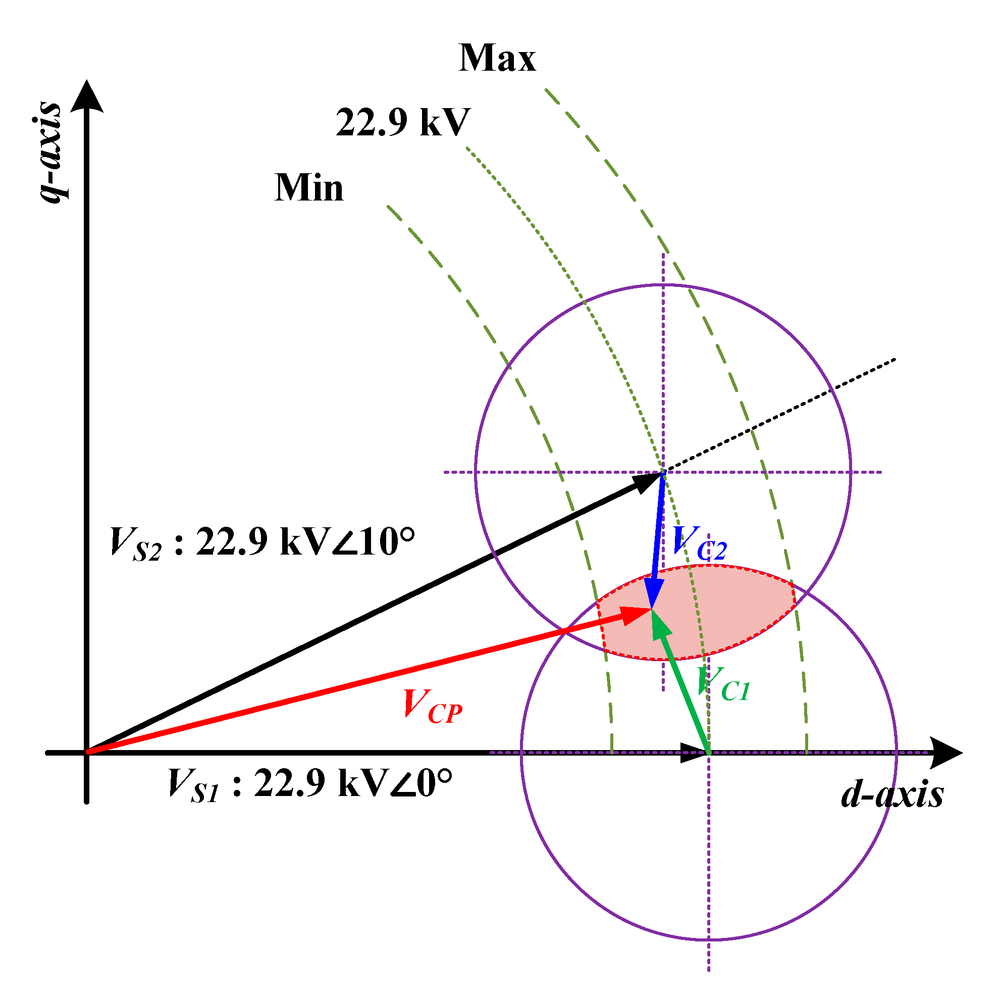
Figure 3 is a vector diagram showing the connection status of distribution lines. It can be seen that the voltage and phase coincide in V_CP. In the vector diagram, the voltage of each substation coincides with 22.9 kV, the phase of substation#1 is 0°, and the phase of substation#2 is 10°; consequently, the phase difference between the two substations is set to 10°.

At this time, the line impedance is ignored because it has a small value compared to the load impedance. In addition, the current flowing into the controller, line current, and load current is always equal owing to the characteristics of the series circuit before the switch is turned ON.

In the vector diagram, the serial compensation voltage (V_C) is the difference between the connection point voltage (V_CP) and the substation voltage (V_S). It can be expressed as follows:

$$V_C\angle {\theta }_C=V_{CP}\angle {\theta }_{CP}-V_S\angle {\theta }_S$$

(1)

Additionally, $\overline{V_C}$ can be expressed using Euler’s formula as given in Equation (2):

$$\overline{V_C}=\left(V_{CP}\cos {\theta }_{CP}+j{V}_{CP}\sin {\theta }_{CP}\right)-\left(V_S\cos {\theta }_S+j{V}_S\sin {\theta }_S\right)$$

(2)

The magnitude and phase of the serial compensation voltage can be expressed by Equations (3) and (4), respectively:

$$V_C=\sqrt{V_{CP}^2+V_S^2-2V_{CP}{V}_S\cos \left({\theta }_{V_{CP}}-{\theta }_{V_S}\right)}$$

(3)

$${\theta }_{V_C}={\tan }^{-1}\left(\frac{V_{CP}\sin {\theta }_{V_{CP}}-V_S\sin {\theta }_{V_S}}{V_{CP}\cos {\theta }_{V_{CP}}-V_S\cos {\theta }_{V_S}}\right)$$

(4)

It can be seen in Equations (3) and (4) that the magnitude and phase of the serial compensation voltage are independent of the magnitude and power factor of the load impedance.

The magnitude and phase of the current flowing into the controller (I_C) can be expressed as given below in Equations (5) and (6):

$$I_C=\frac{1}{Z_L}\sqrt{V_S^2+V_C^2+2V_S{V}_C\cos \left({\theta }_{V_S}-{\theta }_{V_C}\right)}$$

(5)

$${\theta }_{I_C}={\tan }^{-1}\left(\frac{V_S\sin \left({\theta }_{V_S}-{\theta }_{Z_L}\right)-V_C\sin \left({\theta }_{V_C}-{\theta }_{Z_L}\right)}{V_S\cos \left({\theta }_{V_S}-{\theta }_{Z_L}\right)-V_C\cos \left({\theta }_{V_C}-{\theta }_{Z_L}\right)}\right)$$

(6)

Equation (5) shows that the current flowing into the controller varies inversely with the magnitude of the load impedance; however, it is independent of the power factor.

The phase of the current flowing into the controller, provided in Equation (6), varies inversely with the power factor of the load impedance; however, it is independent of the magnitude of the load impedance. Therefore, it can be seen that the current flowing into the controller is correlated with the load impedance.

At this time, the design capacity (P_a) of the APC is as expressed by Equation (7).

$$P_a\left[\mathrm{VA}\right]=V_C\times I_C$$

(7)

It can be seen that P_a is independent of the phase difference between the voltage and the current; therefore, it is not affected by the power factor variation in the load impedance.

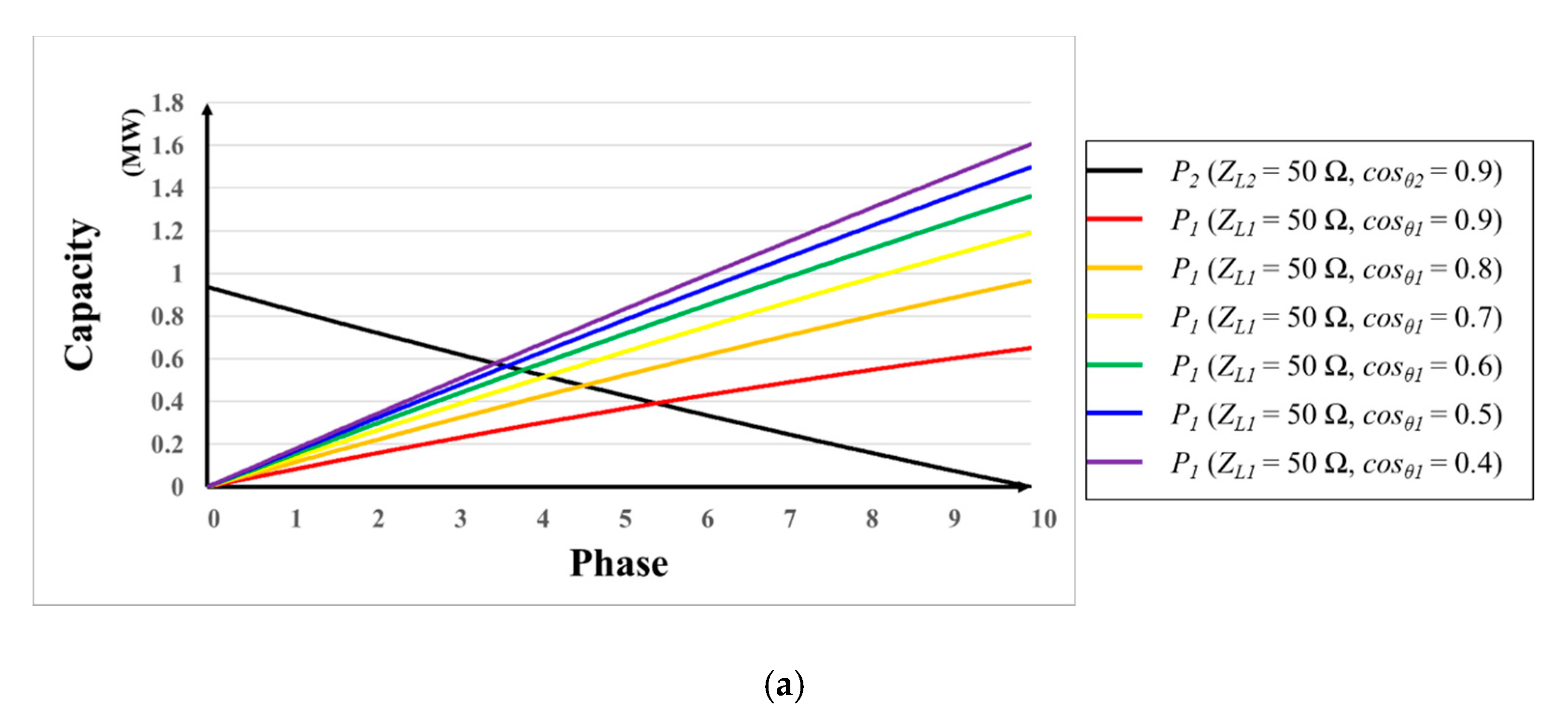
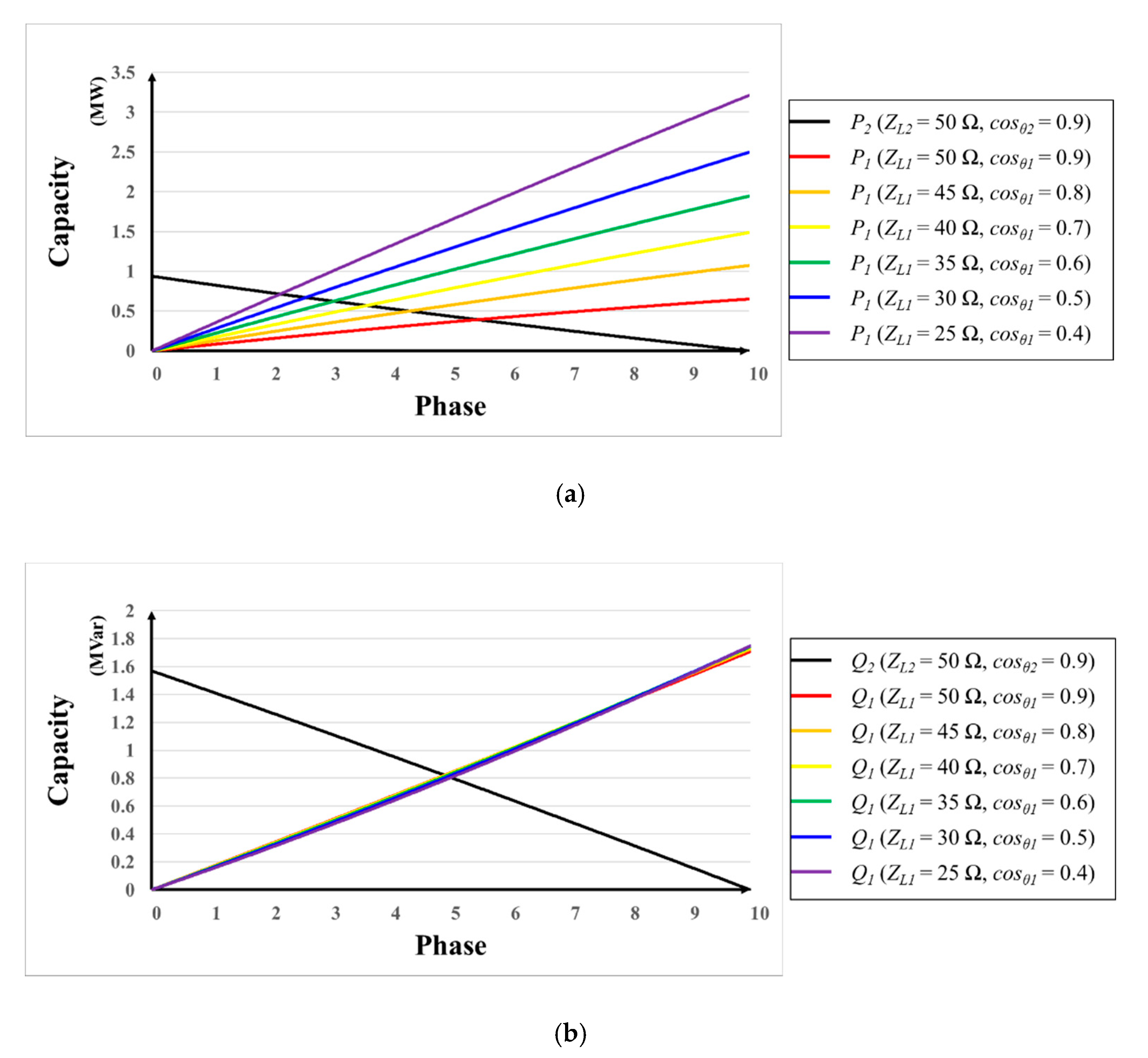
The inductive load occupies a large portion of the distribution line. Considering this, this experiment primarily focused on the lagging load. Figure 4 shows the active power, reactive power, and the apparent power of the APC as the magnitude of the load impedance changes. As mentioned above, the line impedance of the distribution line is not considered. As shown in

Table 1. APC (active phase controller) capacity according to load impedance change when the power factor is constant.

Active Power
Load#2	Z = 50 Ω							PF = 0.9
Load#1	Z	PF	Z	PF	Z	PF	Z	PF	Z	PF	Z	PF	(Ω)
	50	0.9	45	0.9	40	0.9	35	0.9	30	0.9	25	0.9
CP	5.46		5.19		4.89		4.56		4.17		3.73		(°)
P	392		416		444		476		512		555		(kW)
Reactive Power
Load#2	Z = 50 Ω							PF = 0.9
Load#1	Z	PF	Z	PF	Z	PF	Z	PF	Z	PF	Z	PF	(Ω)
	50	0.9	45	0.9	40	0.9	35	0.9	30	0.9	25	0.9
CP	4.89		4.63		4.34		4.01		3.65		3.24		(°)
Q	821		863		909		959		1015		1081		(kVar)
Apparent Power
Load#2	Z = 50 Ω							PF = 0.9
Load#1	Z	PF	Z	PF	Z	PF	Z	PF	Z	PF	Z	PF	(Ω)
	50	0.9	45	0.9	40	0.9	35	0.9	30	0.9	25	0.9
CP	5.00		4.74		4.42		4.12		3.75		3.33		(°)
Pa	915		963		1013		1076		1143		1219		(kVA)

, the magnitude and power factor of load impedance#2 (Z_L2) were assumed constant at 50 Ω and 0.9, respectively, whereas the power factor of load impedance#1 (Z_L1) was fixed at 0.9, and its magnitude was varied for comparative analysis. The x-axis represents the voltage phase coincidence point, and the y-axis represents the output value of the active phase controller.

Figure 4a depicts the active power of the APC as the magnitude of the load impedance#1 (Z_L1) decreases. From Equation (5), it can be seen that the magnitude of the current flowing into the controller increases as the magnitude of the load impedance decreases. Therefore, the active power slope of APC#1 increases.

Figure 4b depicts the reactive power of the APC as the magnitude of the load impedance#1 (Z_L1) decreases. Equation (5) clarifies that the magnitude of the current flowing into the controller increases as the magnitude of the load impedance decreases. Consequently, the reactive power slope of APC#1 increases.

Figure 4c depicts the apparent power of the APC as the magnitude of the load impedance#1 (Z_L1) decreases. As expressed in Equation (5), it can be seen that the magnitude of the current flowing into the controller increases as the magnitude of the load impedance decreases. Therefore, the apparent power slope of APC#1 increases.

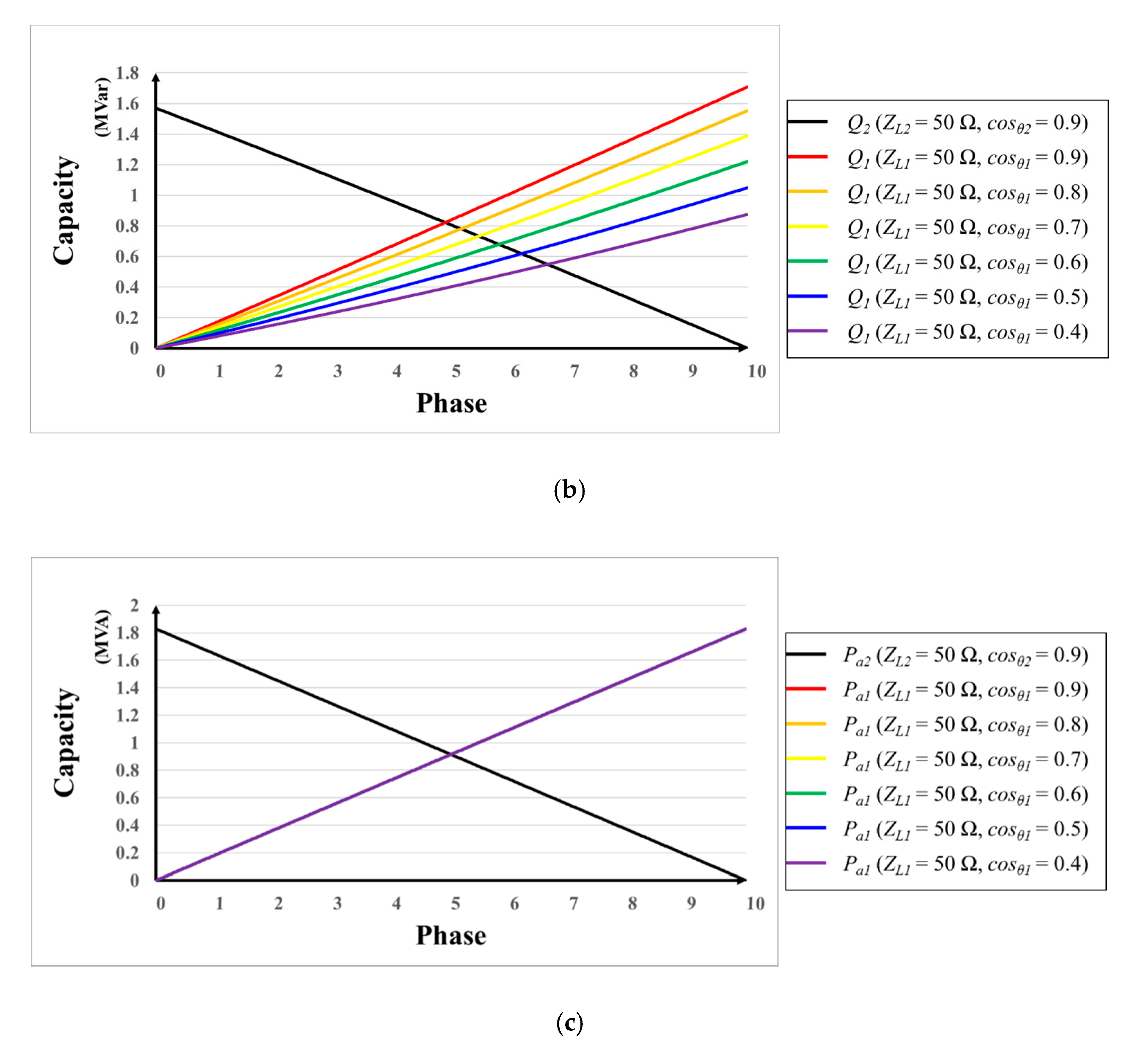
Figure 5 depicts the active power, reactive power, and the apparent power of the APC as the magnitude of the load impedance changes. As shown in

Table 2. APC capacity according to power factor change when the load impedance is constant.

Active Power
Load#2	Z = 50 Ω							PF = 0.9
Load#1	Z	PF	Z	PF	Z	PF	Z	PF	Z	PF	Z	PF	(Ω)
	50	0.9	50	0.8	50	0.7	50	0.6	50	0.5	50	0.4
CP	5.46		4.57		4.11		3.83		3.63		3.50		(°)
P	392		475		518		546		564		578		(kW)
Reactive Power
Load#2	Z = 50 Ω							PF = 0.9
Load#1	Z	PF	Z	PF	Z	PF	Z	PF	Z	PF	Z	PF	(Ω)
	50	0.9	50	0.8	50	0.7	50	0.6	50	0.5	50	0.4
CP	4.89		5.16		5.46		5.80		6.19		6.62		(°)
Q	821		779		732		678		618		548		(kVar)
Apparent Power
Load#2	Z = 50 Ω							PF = 0.9
Load#1	Z	PF	Z	PF	Z	PF	Z	PF	Z	PF	Z	PF	(Ω)
	50	0.9	50	0.8	50	0.7	50	0.6	50	0.5	50	0.4
CP	5		5		5		5		5		5		(°)
Pa	915		915		915		915		915		915		(kVA)

, the magnitude and power factor of load impedance#2 (Z_L2) were assumed constant at 50 Ω and 0.9, respectively, whereas the magnitude of load impedance#1 (Z_L1) was fixed at 50 Ω, and its power factor was varied for comparative analysis.

Figure 5a shows the active power of the APC as the power factor of the load impedance#1 (Z_L1) decreases. Equation (6) clarifies that the phase of the current flowing into the controller increases as the power factor of the load impedance decreases. Therefore, decreasing phase difference between voltage and current results in an increasing active power slope of APC#1.

Figure 5b shows the reactive power of the APC as the power factor of the load impedance#1 (Z_L1) decreases. As expressed in Equation (6), the phase of the current flowing into the controller increases as the power factor of the load impedance decreases. Therefore, decreasing phase difference between voltage and current results in a decreasing reactive power slope of APC#1.

Figure 5c shows the apparent power of the APC as the power factor of the load impedance#1 (Z_L1) decreases. From the results of Equation (7), apparent power remains unaffected by any variation in the phase difference between voltage and current. Therefore, it is independent of the power factor.

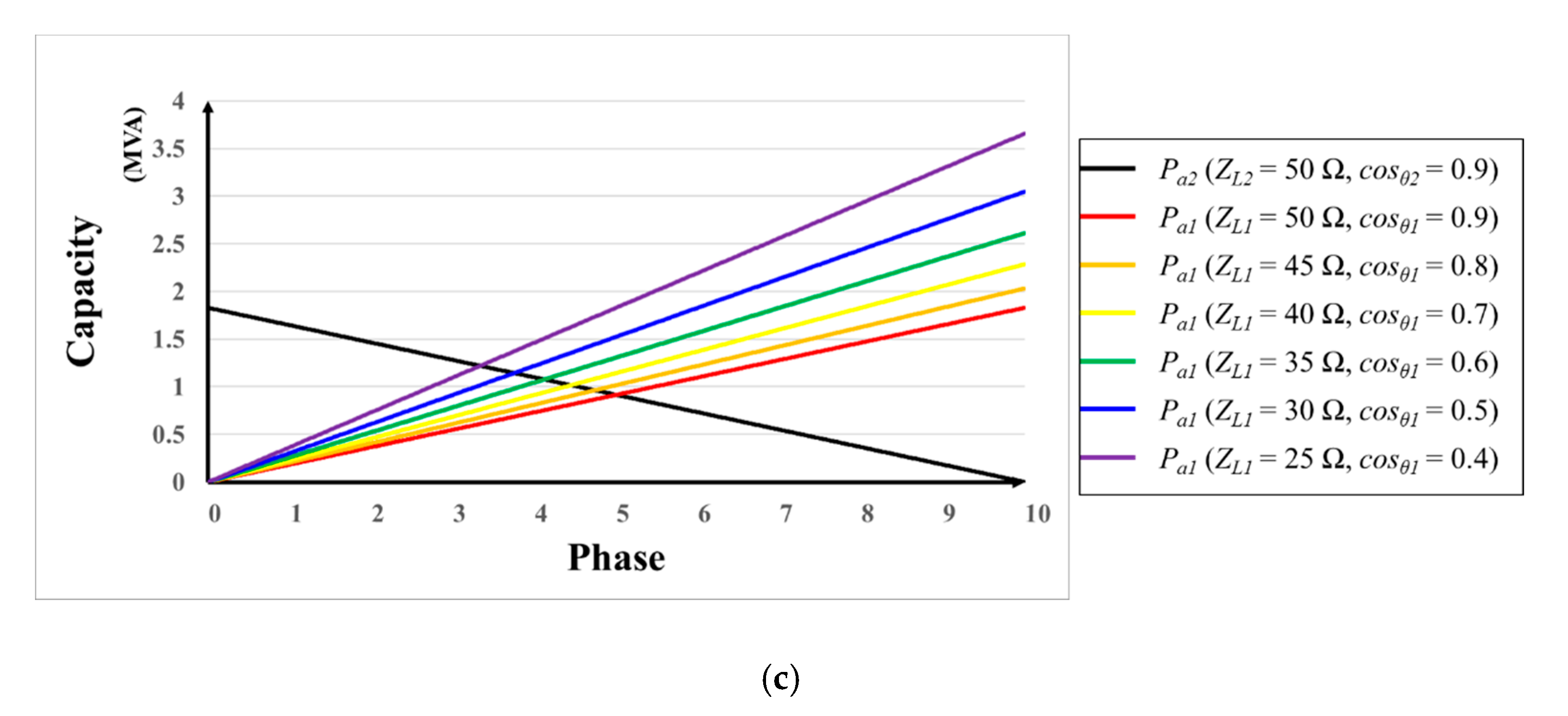
Figure 6 shows the active power, reactive power, and apparent power of the APC against variation in magnitude and power factor of the load impedance. As shown in

Table 3. APC capacity according to load impedance and power factor change.

Active Power
Load#2	Z = 50 Ω							PF = 0.9
Load#1	Z	PF	Z	PF	Z	PF	Z	PF	Z	PF	Z	PF	(Ω)
	50	0.9	45	0.8	40	0.7	35	0.6	30	0.5	25	0.4
CP	5.46		4.31		3.59		3.04		2.57		2.14		(°)
P	392		499		568		623		670		712		(kW)
Reactive Power
Load#2	Z = 50 Ω							PF = 0.9
Load#1	Z	PF	Z	PF	Z	PF	Z	PF	Z	PF	Z	PF	(Ω)
	50	0.9	45	0.8	40	0.7	35	0.6	30	0.5	25	0.4
CP	4.89		4.90		4.91		4.93		4.96		5.00		(°)
Q	821		821		820		817		812		804		(kVar)
Apparent Power
Load#2	Z = 50 Ω							PF = 0.9
Load#1	Z	PF	Z	PF	Z	PF	Z	PF	Z	PF	Z	PF	(Ω)
	50	0.9	45	0.8	40	0.7	35	0.6	30	0.5	25	0.4
CP	5.00		4.74		4.42		4.12		3.75		3.33		(°)
Pa	915		963		1013		1076		1143		1219		(kVA)

, the magnitude and power factor of load impedance#2 (Z_L2) were assumed constant at 50 Ω and 0.9, respectively, whereas those of load impedance#1 (Z_L1) were varied for comparative analysis.

Figure 6a depicts the active power of the APC as the magnitude and power factor of the load impedance#1 (Z_L1) decreases. As mentioned above, the magnitude and phase of the current flowing into the controller increase inversely with the magnitude and power factor of the load impedance#1 (Z_L1). Therefore, the active power slope of APC#1 increases the most steeply owing to an increase in current and a decrease in phase difference.

In Figure 6b, the reactive power of the APC is plotted against the decreasing magnitude and power factor of the load impedance#1 (Z_L1). As mentioned above, the magnitude of the current flowing into the controller increases in inverse proportion to the magnitude of the load impedance#1 (Z_L1). However, the phase difference due to the phased reduction of the current decreases. Therefore, it can be seen that the reactive power slope of APC#1 is maintained almost constant.

In Figure 6c, the apparent power of the APC is plotted against decreasing magnitude and power factor of the load impedance#1 (Z_L1). As mentioned above, apparent power is not affected by the phase difference between voltage and current; therefore, the result is similar to that observed in Figure 4c.

Figure 7 shows the outputs of APC#1 and APC#2 based on the parameters applied to the simulation in

Table 4. Distribution Line Parameters.

10 MW	V		Phase
Substation#1, VS1	22.9 kV		0$°$
Substation#2, VS2	22.9 kV		10$°$
	Z	PF	R	L
Load#1, ZL1	40 $\mathsf{\Omega }$	0.7	28 $\mathsf{\Omega }$	75.77 mH
Load#2, ZL2	50 $\mathsf{\Omega }$	0.9	45 $\mathsf{\Omega }$	57.81 mH

.

Table 5. Output of APC according to controlled phase.

Phase		APC#1	APC#2	Total
0	(°)	0	1830	1830	(kVA)
4.42	(°)	1013	1013	2026	(kVA)
7	(°)	1603	550	2153	(kVA)
10	(°)	2282	0	2282	(kVA)

shows the capacity of each APC according to the phase matching point. When the voltage phase between distribution lines is matched at 0°, APC#1 does not function; as a result, the output of APC#1 is 0 kVA. In this case, the voltage phase is matched by driving only the APC#2; consequently, the output of APC#2 is 1830 kVA. Moreover, the total APC synthesis capacity is approximately 1830 kVA, which is the smallest value. However, in order to operate the system efficiently, APC#2 must accommodate all the phase control burdens.

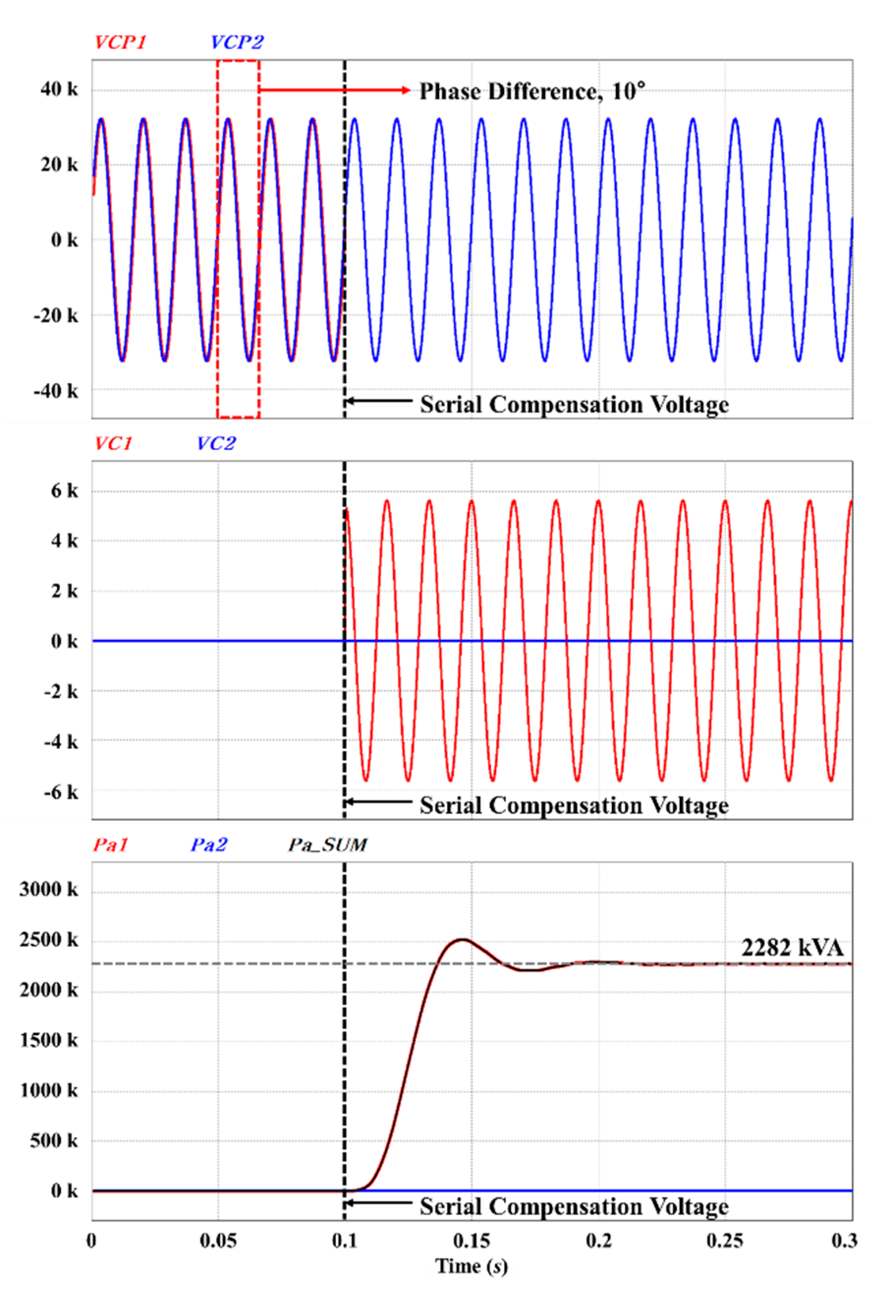
When the voltage phase between distribution lines is matched at 10°, APC#2 does not function; hence, the output of APC#2 is 0 kVA. In this case, the voltage phase is matched by driving only APC#1, and the output of APC#1 is 2282 kVA. Moreover, the total APC synthesis capacity is approximately 2282 kVA, which is the highest value.

Furthermore, if the voltage phases match at 4.42°, where the outputs of APC#1 and APC#2 are the same, the synthesis capacity is 2026 kVA and is higher than that if they match at 0°. However, the outputs of both the APCs are the same; consequently, an efficient design can be realized. Therefore, it is important to derive a voltage phase matching point at which the output is not to be concentrated on one side and can be shared uniformly. Moreover, it can be seen from Figure 7 that the output is the same at the point where the output waveforms of the APCs intersect.

As mentioned above, the line impedance of each distribution line is ignored, and all impedances in the path are replaced by a single impedance. Therefore, it can be expressed as shown in Equation (8), where the outputs of APC#1 and APC#2 are equal.

$$P_{a_1}=V_{C_1}{I}_{C_1}=V_{C_2}{I}_{C_2}=P_{a_2}$$

(8)

Moreover, as shown in Figure 3, each serial compensation voltage can be represented by the difference between the connection point voltage and the substation voltage. In addition, owing to the nature of the series circuit, the current flowing into the controller is the same as the line current; consequently, it is equal to the current flowing into the load impedance according to Ohm’s law.

$$V_C=V_{CP}-V_S$$

(9)

$$I_C=\frac{V_{CP}}{Z_L}$$

(10)

Using these values, Equation (8) can be modified as follows:

$$\left(V_{CP}-V_{S_1}\right)\times \frac{V_{CP}}{Z_{L_1}}=\left(V_{CP}-V_{S_2}\right)\times \frac{V_{CP}}{Z_{L_2}}$$

(11)

Furthermore, when Equation (11) is expressed as a function of V_CP, the optimal connection point voltage can be expressed as follows:

$$V_{CP}=\frac{Z_{L_2}{V}_{S_1}-Z_{L_1}{V}_{S_2}}{Z_{L_2}-Z_{L_1}}$$

(12)

If line current detection is possible through the current sensor located at the APC output terminal, Equation (11) can be expressed as Equation (13).

$$\left(V_{CP}-V_{S_1}\right)\times I_{C_1}=\left(V_{CP}-V_{S_2}\right)\times I_{C_2}$$

(13)

Therefore, the optimal connection point voltage can be expressed as follows:

$$V_{CP}=\frac{V_{S_1}{I}_{C_1}-V_{S_2}{I}_{C_2}}{I_{C_1}-I_{C_2}}$$

(14)

Moreover, when the reference value calculated from Equation (12) is applied to the APC, it can be seen that the outputs of the APC coincides with each other at 4.42°.

In Figure 8, the magnitude and phase of the voltage at substation#1 are 22.9 kVA and 0°, respectively, whereas those at substation#2 are 22.9 kVA and 15°, respectively. This is the case when the phase difference between the lines is larger than that originally expected after the APC was installed, and the output of the APC is insufficient. As shown in Figure 8, the voltage phase must match the phase at the V_CP, but it is impossible because the output of the APC is insufficient.

However, the standard of the 1.5–10 MVA class distribution line is within 10°. Therefore, there is no need to match the voltage phase accurately in V_CP.

In Figure 9, each APC is driven at maximum operation, which not only satisfies the standard specifications but also minimizes the voltage phase difference between the lines. As shown in the figure, each line voltage was moved to V_CP1 and V_CP2 through the maximum operation of the APC. Moreover, in order to achieve the optimum connection point voltage (V_CP), which was calculated from Equations (3) and (4), the magnitude and phase of the serial compensation voltage (V^’_C1) are 2545.76 V and 105.97°, respectively, whereas those of the serial compensation voltage (V^’_C2) are 3182.19 V and −93.76°, respectively. Therefore, when the maximum output voltage of the APC is designed as 2000 V, the magnitude and phase of the serial compensation voltage (V_C1) are 2000 V and 105.97°, respectively.

The magnitude and phase of the serial compensation voltage (V_C1) are 2000 V and −93.76°, respectively. By modifying the second law of cosines as shown in Equations (15) and (16), the voltages V_CP1 and V_CP2 of each connection point can be calculated.

$$V_{CP1}=\sqrt{V_{S1}^2+V_{C1}^2-2V_{S1}{V}_{C1}\cos {\theta }_1}$$

(15)

$$V_{CP2}=\sqrt{V_{S2}^2+V_{C2}^2-2V_{S2}{V}_{C2}\cos {\theta }_2}$$

(16)

θ₁ and θ₂ in the above equations can be obtained from Equations (17) and (18):

$${\theta }_1=180-{\theta }_{C1}$$

(17)

$${\theta }_2=180-{\theta }_{S2}-{\theta }_{C2}$$

(18)

In addition, the values of θ₁ and θ₂ obtained from Equations (15) and (16) are the same as those obtained using Equations (19) and (20):

$${\theta }_1={\cos }^{-1}\left(\frac{V_{S1}^2+V_{C1}^2-V_{CP1}^2}{2V_{S1}{V}_{C1}}\right)$$

(19)

$${\theta }_2={\cos }^{-1}\left(\frac{V_{S2}^2+V_{C2}^2-V_{CP2}^2}{2V_{S2}{V}_{C2}}\right)$$

(20)

Therefore, V_CP1 and V_CP2 can be expressed using Equations (21) and (22), respectively, as follows:

$$V_{CP1}=\sqrt{V_{S1}^2+V_{C1}^2-2V_{S1}{V}_{C1}\cos \left(180-{\theta }_{C1}\right)}$$

(21)

$$V_{CP2}=\sqrt{V_{S2}^2+V_{C2}^2-2V_{S2}{V}_{C2}\cos \left(180-{\theta }_{S2}-{\theta }_{C2}\right)}$$

(22)

By modifying the second law of cosines, as shown in Equations (23) and (24), respectively, the phases θ_CP1 and θ_CP2 of each connection point were calculated.

$${\theta }_{CP1}={\cos }^{-1}\left(\frac{V_{S1}^2+V_{CP1}^2-V_{C1}^2}{2V_{S1}{V}_{CP1}}\right)$$

(23)

$${\theta }_{CP2}={\theta }_{S2}-{\cos }^{-1}\left(\frac{V_{S2}^2+V_{CP2}^2-V_{C2}^2}{2V_{S2}{V}_{CP2}}\right)$$

(24)

Therefore, V_CP1 and V_CP2 can be finally expressed, respectively, by Equations (25) and (26):

$$V_{CP1}\angle {\theta }_{CP1}=\sqrt{V_{S1}^2+V_{C1}^2-2V_{S1}{V}_{C1}\cos \left(180-{\theta }_{C1}\right)}\angle {\cos }^{-1}\left(\frac{V_{S1}^2+V_{CP1}^2-V_{C1}^2}{2V_{S1}{V}_{CP1}}\right)$$

(25)

$$V_{CP2}\angle {\theta }_{CP2}=\sqrt{V_{S2}^2+V_{C2}^2-2V_{S2}{V}_{C2}\cos \left(180-{\theta }_{S2}-{\theta }_{C2}\right)}\angle \left({\theta }_{S2}-{\cos }^{-1}\left(\frac{V_{S2}^2+V_{CP2}^2-V_{C2}^2}{2V_{S2}{V}_{CP2}}\right)\right)$$

(26)

Figure 10 depicts the case where the phase of substation#1 has a value other than 0°. In this case, θ₁ can be calculated as follows:

$${\theta }_1=180-{\theta }_{C1}+{\theta }_{S1}$$

(27)

Furthermore, by modifying the second law of cosines, as provided below in Equations (28) and (29), the voltages V_CP1 and V_CP2 of each connection point were calculated.

$$V_{CP1}=\sqrt{V_{S1}^2+V_{C1}^2-2V_{S1}{V}_{C1}\cos \left(180-{\theta }_{C1}+{\theta }_{S1}\right)}$$

(28)

$$V_{CP2}=\sqrt{V_{S2}^2+V_{C2}^2-2V_{S2}{V}_{C2}\cos \left(180-{\theta }_{S2}-{\theta }_{C2}\right)}$$

(29)

The value of θ_CP1 can be obtained from Equation (30).

$${\theta }_{CP1}={\theta }_{S1}+{\cos }^{-1}\left(\frac{V_{S1}^2+V_{CP1}^2-V_{C1}^2}{2V_{S1}{V}_{CP1}}\right)$$

(30)

Therefore, V_CP1 and V_CP2 can be finally expressed by Equations (31) and (32).

$$V_{CP1}\angle {\theta }_{CP1}=\sqrt{V_{S1}^2+V_{C1}^2-2V_{S1}{V}_{C1}\cos \left(180-{\theta }_{C1}+{\theta }_{S1}\right)}\angle \left({\theta }_{S1}+{\cos }^{-1}\left(\frac{V_{S1}^2+V_{CP1}^2-V_{C1}^2}{2V_{S1}{V}_{CP1}}\right)\right)$$

(31)

$$V_{CP2}\angle {\theta }_{CP2}=\sqrt{V_{S2}^2+V_{C2}^2-2V_{S2}{V}_{C2}\cos \left(180-{\theta }_{S2}-{\theta }_{C2}\right)}\angle \left({\theta }_{S2}-{\cos }^{-1}\left(\frac{V_{S2}^2+V_{CP2}^2-V_{C2}^2}{2V_{S2}{V}_{CP2}}\right)\right)$$

(32)

3. Simulation Verification

The output of APC according to the variation in the reference value of the connection point voltage was measured. The voltage phase coincidence points were set to 0°, 4.42°, 7° and 10°. After 0.1 s, the output voltage of the APC was applied to the distribution line. The magnitude of each substation voltage was ensured to be 22.9 kV with a phase difference of 10°. Furthermore, the connection point voltage was kept equal to the substation voltage in parallel. In Figure 11, the simulation result waveforms are plotted considering the voltage phase coincidence point as 0°. Moreover, the phase of the connection point voltage (V_CP1) was set as 0°, to ensure that APC#1 was not driven and that the serial compensation voltage (V_C1) was 0 V. Therefore, the voltage phase between the lines could be matched only by driving APC#2. Furthermore, the synthesis capacity of APC was measured to be 1830 kVA, which was the lowest. Figure 12 depicts the simulation result waveform when the voltage phase coincidence point was set to 20°. In this case, the phase of the connection point voltage (V_CP2) was at 10°; consequently, APC#2 was not driven, and, hence, the serial compensation voltage (V_C2) was 0 V. Therefore, the voltage phase between the lines was matched by driving only APC#1. Moreover, the synthesis capacity of the APC, in this case, was measured to be 2282 kVA, which was the highest. In conclusion, if only one APC is used, it can be constructed with the lowest capacity if it is designed considering APC#2.

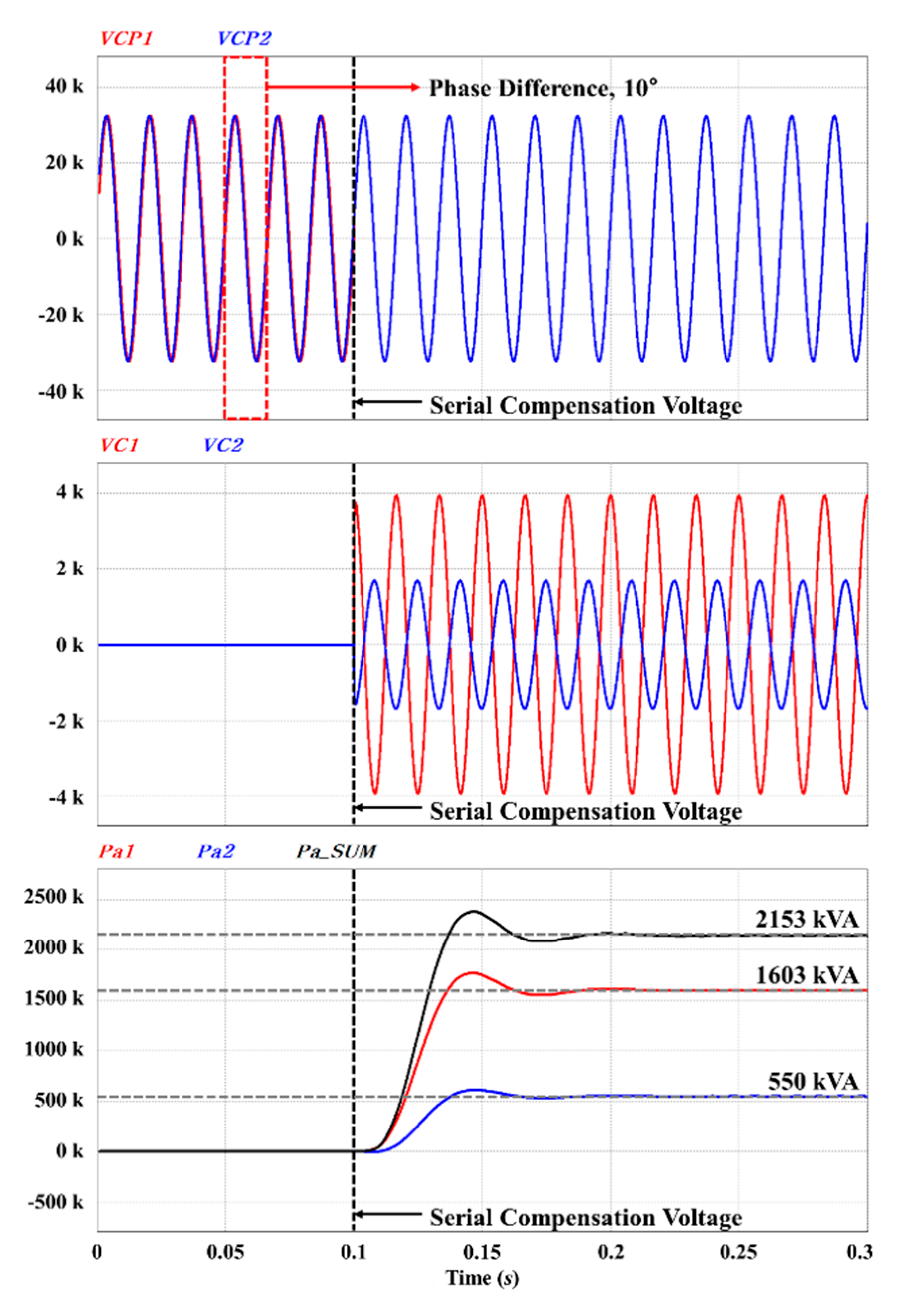
In Figure 13, the simulation result waveforms are plotted considering the voltage phase coincidence point to be 7°. The connection point voltages between the distribution lines are equal; however, the outputs of the APCs are different. The capacities of APC#1 and APC#2 are 1603 kVA and 550 kVA, respectively. Moreover, the output gap between the APCs is large. In this case, the circuit design is difficult because different parameter values are required for the configuration of the controller circuit. Furthermore, when the APC is designed with the same parameter values, the output of APC#1 is smaller than its design capacity, thus resulting in lower output due to overdesign.

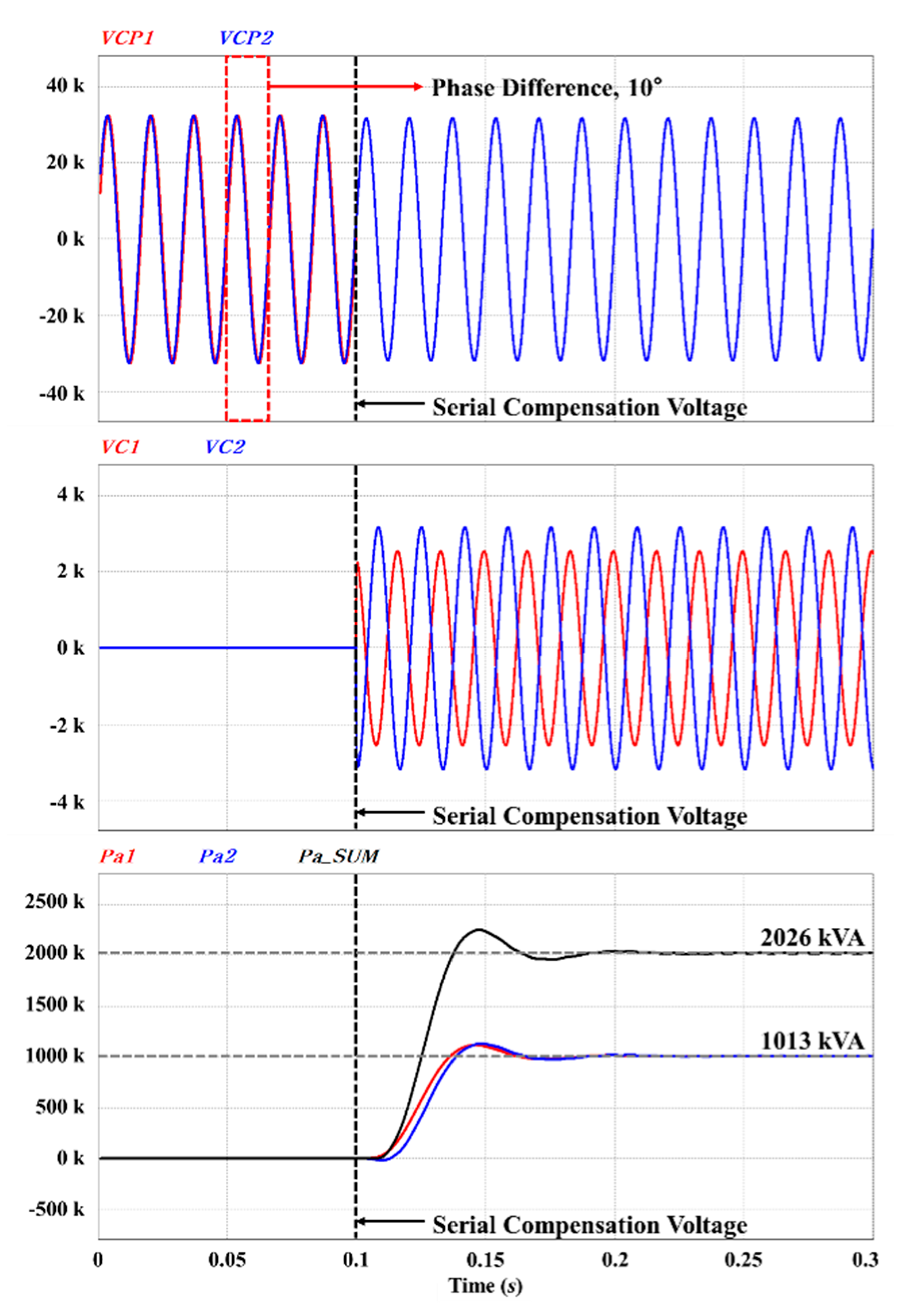
In Figure 14, the simulation result waveforms are plotted considering the voltage phase coincidence point as 4.42°. The reference value of the connection point voltage calculated from Equation (12) was applied to the controller. It can be seen that not only the voltages between the lines coincide with each other, but the outputs of both the APCs are 1013 kVA. The synthetic capacity of APC is 2026 kVA, which is somewhat higher than that in case of matching the phase at 0°. However, the output of the APC is evenly distributed, and efficient operation is possible. In the simulation results, the capacity of the controller differs according to the voltage phase coincidence point, and the magnitude of the serial compensation voltage increases as the interval to reach the coincidence point increases.

4. Conclusions

In this paper, a capacity calculation method for an active phase controller is proposed, which can help suppress the circulating current caused by the potential difference between connection points during the autonomous reconfiguration of a line. Existing FACTSs (flexible AC transmission systems), such as UPQCs (unified power quality conditioners) and UPFCs (unified power flow controllers), are designed for power flow control of the transmission line; thus, the design capacity is large, and the cost is high accordingly. However, the proposed APC controls only the phase angle of within 10° for the connection point; thus, it requires a small power capacity compared with conventional UPQC and UPFC. When calculating the capacity of the APC, the magnitude and phase of the current flowing into the APC was found to increase inversely with the magnitude and power factor of the path impedance, which greatly contributed to the increase in the output of the APC. In addition, the output of APC was calculated differently according to the phase change of the connection point voltage. Therefore, it was possible to operate an efficient APC by calculating the optimal connection point voltage through the proposed formula. Moreover, it was also possible to contribute to reducing the controller design cost by calculating the optimal APC capacity. Finally, the proposed control technique was validated using simulation.

In the future, it will be necessary to develop a control algorithm that can calculate the optimal connection point voltage even in the unbalanced load state of the distribution line.

References

- Chaichana, A.; Syed, M.H.; Burt, G.M. Vulnerability mitigation of transmission line outages using demand response approach with distribution factors. In Proceedings of the 2016 IEEE 16th International Conference on Environment and Electrical Engineering (EEEIC), Florence, Italy, 7–10 June 2016; pp. 1–6. [Google Scholar]
- Ahmad, S.; Albatsh, F.M.; Mekhilef, S.; Mokhlis, H. An approach to improve active power flow capability by using dynamic unified power flow controller. In Proceedings of the 2014 IEEE Innovative Smart Grid Technologies-Asia (ISGT ASIA), Kuala Lumpur, Malaysia, 20–23 May 2014; pp. 249–254. [Google Scholar]
- Uno, Y.; Fujita, G.; Yokoyama, R.; Matubara, M.; Toyoshima, T.; Tsukui, T. Evaluation of micro-grid supply and demand stability for different interconnections. In Proceedings of the 2006 IEEE International Power and Energy Conference, Putra Jaya, Malaysia, 28–29 November 2006; pp. 612–617. [Google Scholar]
- Mustafa, U.; Arif, M.S.B.; Rahman, H.; Sidik, M.A.B. Modelling and optimization of simultaneous AC-DC transmission to enhance power transfer capacity of the existing transmission lines. In Proceedings of the 2017 International Conference on Electrical Engineering and Computer Science (ICECOS), Palembang, Indonesia, 22–23 August 2017; pp. 328–332. [Google Scholar]
- Murugan, A.; Thamizmani, S. A new approach for voltage control of IPFC and UPFC for power flow management. In Proceedings of the 2013 International Conference on Energy Efficient Technologies for Sustainability, Nagercoil, India, 10–12 April 2013; pp. 1376–1381. [Google Scholar]
- Hasheminamin, M.; Agelidis, V.G.; Salehi, V.; Teodorescu, R.; Hredzak, B. Index-based assessment of voltage rise and reverse power flow phenomena in a distribution feeder under high PV penetration. IEEE J. Photovoltaics 2015, 5, 1158–1168. [Google Scholar] [CrossRef]
- Holguin, J.P.; Rodriguez, D.C.; Ramos, G. Reverse Power Flow (RPF) detection and impact on protection coordination of distribution systems. IEEE Trans. Ind. Appl. 2020, 56, 2393–2401. [Google Scholar] [CrossRef]
- Nguyen, H.D.; Turitsyn, K. Voltage multistability and pulse emergency control for distribution system with power flow reversal. IEEE Trans. Smart Grid. 2015, 6, 2985–2996. [Google Scholar] [CrossRef] [Green Version]
- Lee, S.; Yang, M.U.; Kim, K.J.; Yoon, Y.T.; Moon, S.; Park, J. Smart-grid based substation testing simulator design for the South Korean power distribution system. In Proceedings of the 2013 IEEE Power & Energy Society General Meeting, Vancouver, BC, Canada, 21–25 July 2013; pp. 1–5. [Google Scholar]
- Wen, W.; Wei, L.; Wenjun, D.; Xiao, M. Design and analysis for reliability of control function in substation automation. In Proceedings of the 2006 International Conference on Power System Technology, Chongqing, China, 22–26 October 2006; pp. 1–4. [Google Scholar]
- Liu, Y.; Su, J.; Liu, F. Design about real-time fault detection information system of the transformer substation. In Proceedings of the 2009 International Conference on Computer Engineering and Technology, Singapore, 22–24 January 2009; pp. 197–200. [Google Scholar]
- Du, C.; Liang, X.; Li, S. An optimized design of slobozhanska substation with high renewable energy penetration. In Proceedings of the 2019 IEEE Sustainable Power and Energy Conference (iSPEC), Beijing, China, 21–23 November 2019; pp. 153–157. [Google Scholar]
- Gogan, P.L.; Wyckoff, G.D. Design and construction of sustainable substations. In Proceedings of the PES T&D, Orlando, FL, USA, 7–10 May 2012; pp. 1–4. [Google Scholar]
- Jijun, Z.; Jianfeng, G.; Xiaobo, H. Study on network design of automation system in smart substation. In Proceedings of the CICED 2010, Nanjing, China, 13–16 September 2010; pp. 1–5. [Google Scholar]
- Tamizkar, R.; Javadian, S.A.M.; Haghifam, M. Distribution system reconfiguration for optimal operation of distributed generation. In Proceedings of the 2009 International Conference on Clean Electrical Power, Capri, Italy, 9–11 June 2009; pp. 217–222. [Google Scholar]
- Polat, O.; Nasibov, F.; Hasancebi, G.; Gul, O. Wide area autonomous restoration system for medium voltage distribution networks. In Proceedings of the 2018 International Conference and Exposition on Electrical and Power Engineering (EPE), Iasi, Romania, 18–19 October 2018; pp. 470–474. [Google Scholar]
- Hegny, I.; Holzer, R.; Grabmair, G.; Zoitl, A.; Auinger, F.; Wahlmuller, E. A distributed energy management approach for Autonomous Power Supply Systems. In Proceedings of the 2007 5th IEEE International Conference on Industrial Informatics, Vienna, Austria, 23–27 June 2007; pp. 1065–1070. [Google Scholar]
- Yasar, M.; Beytin, A.; Bajpai, G.; Kwatny, H.G. Integrated Electric Power System supervision for reconfiguration and damage mitigation. In Proceedings of the 2009 IEEE Electric Ship Technologies Symposium, Baltimore, MD, USA, 20–22 April 2009; pp. 345–352. [Google Scholar]
- Wang, J.; Wang, W.; Yuan, Z.; Wang, H.; Wu, J. A chaos disturbed beetle antennae search algorithm for a multiobjective distribution network reconfiguration considering the variation of load and DG. IEEE Access 2020, 8, 97392–97407. [Google Scholar] [CrossRef]
- Qin, X. Study of the application of active power adjustment and control technology based on modem energy storage into power system stability control and voltage adjustment. In Proceedings of the 2014 International Conference on Power System Technology, Chengdu, China, 20–22 October 2014; pp. 1–6. [Google Scholar]
- Zhan, S.; Xinzhan, L.; Yu, H.; Ying, W. Real-time active power control method of regional power grid considering wind power fluctuations under CPS framework. In Proceedings of the 2018 International Conference on Power System Technology (POWERCON), Guangzhou, China, 6–8 November 2018; pp. 2979–2983. [Google Scholar]
- Ding, K.; Liu, J.; Wang, X.; Zhang, X.; Wang, N. Research of an active and reactive power coordinated control method for photovoltaic inverters to improve power system transient stability. In Proceedings of the 2016 China International Conference on Electricity Distribution (CICED), Xi’an, China, 10–13 August 2016; pp. 1–5. [Google Scholar]
- Kabir, M.A.; Mahbub, U. Synchronous detection and digital control of Shunt Active Power Filter in power quality improvement. In Proceedings of the 2011 IEEE Power and Energy Conference at Illinois, Champaign, IL, USA, 25–26 February 2011; pp. 1–5. [Google Scholar]
- Zhou, L.; Qi, S.; Huang, L.; Zhou, Z.; Zhu, Y. Design and simulation of a Control System with a comprehensive power quality in Power System. In Proceedings of the 2007 International Conference on Electrical Machines and Systems (ICEMS), Seoul, Korea, 8–11 October 2007; pp. 376–381. [Google Scholar]
- Huan, H. Research on power quality control method of active distribution network with microgrids. In Proceedings of the 2018 3rd International Conference on Smart City and Systems Engineering (ICSCSE), Xiamen, China, 29–30 December 2018; pp. 533–536. [Google Scholar]
Figure 1.
Diagram representing connections between the distribution lines.
Figure 2.
Distribution system reconfiguration: (a) before; (b) after.
Figure 3.
Vector diagram of the distribution line.
Figure 4.
APC (active phase controller) capacity according to load impedance variation when the lagging power factor (PF = 0.9) is constant. (a) Active power; (b) reactive power; (c) apparent power.
Figure 5.
APC capacity according to power factor change when the load impedance is constant. (a) Active power; (b) reactive power; (c) apparent power.
Figure 6.
APC capacity according to load impedance and power factor change. (a) Active power; (b) reactive power; (c) apparent power.
Figure 7.
Total APC capacity according to load impedance and power factor variation.
Figure 8.
Vector diagram of the distribution line when the maximum output voltage of the APC is exceeded (when the phase of VS1 is 0°).
Figure 9.
Parameter extraction for calculation of VCP1 and VCP2.
Figure 10.
Vector diagram of the distribution line when the maximum output voltage of the APC is exceeded (when the phase of VS1 is not 0°).
Figure 11.
Connection point voltage and APC capacity at the controlled angle of 0°.
Figure 12.
Connection point voltage and APC capacity at the controlled angle of 10°.
Figure 13.
Connection point voltage and APC capacity at the controlled angle of 7°.
Figure 14.
Connection point voltage and APC capacity at the controlled angle of 4.42°.