On Some Symmetries of Quadratic Systems

Abstract

We provide a general method for identifying real quadratic polynomial dynamical systems that can be transformed to symmetric ones by a bijective polynomial map of degree one, the so-called affine map. We mainly focus on symmetry groups generated by rotations, in other words, we treat equivariant and reversible equivariant systems. The description is given in terms of affine varieties in the space of parameters of the system. A general algebraic approach to find subfamilies of systems having certain symmetries in polynomial differential families depending on many parameters is proposed and computer algebra computations for the planar case are presented.

1. Introduction

Studying various symmetries of dynamical systems is important for several reasons. Systems which phase diagrams posses a rotational symmetry are interesting because they are related to the second part of Hilbert’s 16th problem and the existence of such systems can lead to the construction of families with many limit cycles. Another reason for investigation of symmetries is their connection with the integrability. It is well known that an elementary singular point of a time-reversible polynomial system of degree two is always integrable [1]. It can be either a center or an integrable saddle [2] and it thus cannot be a focus. A similar conclusion is valid for much larger families of systems, as it had been shown in [2] where we found affine varieties in the space of parameters of a quadratic planar system which can be brought to a time-reversible one by a bijective linear transformation. This transformation preserves the integrability property of a present singular point at the origin. So, if the quadratic planar system with an isolated non-degenerate trace-zero singular point at the origin admits the transformation to a time-reversible system, the origin is automatically integrable.

In this paper we firstly treat affine transformations to symmetric systems (n-dimensional, $n\ge 2$) in a unified and rather general way. Secondly, for planar quadratic systems, we calculate the varieties in the space of parameters defining the systems which can be transformed to rotationally (reversible) equivariant systems by an affine or merely linear (i.e., no translation involved) transformation.

Let us add some notation. All vectors from ${\mathbb{R}}^n$ will be typeset in boldface. When we mention a linear map from ${\mathbb{R}}^n\to {\mathbb{R}}^n$, we have in mind an additive homogeneous (of degree one) map (which sends 0 to 0). By an affine map we denote a composition of a linear map and a translation. Linear maps will be denoted by capital letters and general (not necessarily linear) maps in calligraphic font. The symbols Id or ${\mathrm{Id}}_n$ will both stand for the identity matrix and the transposition of a matrix A.

Our paper is organized as follows—in Section 2 we describe the general properties of (reversible) symmetric systems in ${\mathbb{R}}^n$ and in Section 3 we compute algebraic varieties in parameter space, corresponding to quadratic planar systems that can be transformed to the (reversible) symmetric one by an affine or linear transformation. With some examples in Section 3 we end the paper.

2. Equivariant and Reversible Equivariant Systems in ${\mathbb{R}}^n$

Let us start with a rather general definition of a symmetry of a dynamical system. Throughout the paper, we will be interested in smooth, mostly polynomial dynamical systems of the form

$$\frac{d\mathbf{x}}{dt}=\mathcal{F}\left(\mathbf{x}\right),\mathbf{x}\left(t\right)\in {\mathbb{R}}^n.$$

(1)

Following Lamb et al. [3,4], we say that a bijective map $\mathcal{B}:{\mathbb{R}}^n\to {\mathbb{R}}^n$ is a symmetry of the system (1) when

$$\frac{d(\mathcal{B}\circ \phi )}{dt}=\mathcal{F}\circ \mathcal{B}\circ \phi$$

(2)

for each trajectory $\phi :t\mapsto \mathbf{x}\left(t\right)$ of system (1). A map $\mathcal{C}:{\mathbb{R}}^n\to {\mathbb{R}}^n$ is called a reversible symmetry of system (1) when

$$\frac{d(\mathcal{C}\circ \phi )}{dt}=-\mathcal{F}\circ \mathcal{C}\circ \phi$$

(3)

for each trajectory $\phi$ of (1). The condition (2) implies that the system is invariant under transformation $(\mathbf{x},t)\mapsto \left(\mathcal{B}\right(\mathbf{x}),t)$ and (3) implies the invariance under the map $(\mathbf{x},t)\mapsto \left(\mathcal{C}\right(\mathbf{x}),-t)$.

We will be only interested in linear (reversible) symmetries. Let $B:{\mathbb{R}}^n\to {\mathbb{R}}^n$ be a linear map. Then, by the linearity, $\frac{d(B\circ \phi )}{dt}=B\frac{d\phi }{dt}=\mathcal{F}\circ \phi \left(t\right)$. Now, if for some regular $n\times n$ matrix B and a fixed $\epsilon \in \{1,-1\}$

$$\mathcal{F}\left(B\mathbf{x}\right)=\epsilon B\mathcal{F}\left(\mathbf{x}\right)$$

(4)

holds for every $\mathbf{x}\in {\mathbb{R}}^n$, then B is a symmetry if $\epsilon =1$, and it is a reversible symmetry if $\epsilon =-1$.

Let $\Gamma$ be a finite cyclic group of invertible linear operators (matrices) on ${\mathbb{R}}^n$. It is said that system (1) is $\Gamma$-equivariant if every $B\in \Gamma$ is a symmetry of the system. Further, it is said that a system (1) is reversible $\Gamma$-equivariant if there exists a non-trivial homomorphism $\sigma :\Gamma \to \{-1,1\}$ such that for every $B\in \Gamma$,

$$\mathcal{F}\left(B\mathbf{x}\right)=\sigma \left(B\right)B\mathcal{F}\left(\mathbf{x}\right)$$

(5)

holds true for every $\mathbf{x}\in {\mathbb{R}}^n$. Obviously, the elements $B\in \Gamma$ for which $\sigma \left(B\right)=-1$, are reversing symmetries and those B with $\sigma \left(B\right)=1$ are symmetries. By the successive application of (5), we get

$$\mathcal{F}\left(B^k\mathbf{x}\right)=\sigma {\left(B\right)}^k{B}^k\mathcal{F}\left(\mathbf{x}\right)$$

(6)

for all $\mathbf{x}\in {\mathbb{R}}^n$ and for all integers k. It easily follows that all even powers of a reversible symmetry are symmetries and all odd powers of a reversible symmetry are reversible symmetries. Therefore, in order that there exists a non-trivial reversible $\Gamma$-equivariant system, the order of $\Gamma$ must be even as it can be easily seen by inserting the order of $\Gamma$ for k in (6).

In the next proposition we will see that having only information for a generator of the group suffices.

Proposition 1.

A system (1) is Γ-equivariant if and only if any fixed generator of Γ is a symmetry. A system (1) is reversible Γ-equivariant if and only if some fixed generator of Γ is a reversible symmetry.

Proof. 

By application of (6) and taking $\sigma \left(R\right)=-1$ for the chosen generator R of $\Gamma$ in the reversible case, the claims easily follow. □

We recall the definition of Kronecker product of matrices related to the tensor product of operators. The Kronecker product of $A=\left[a_{ij}\right]\in {\mathbb{R}}^{m,n}$ and $B=\left[b_{ij}\right]\in {\mathbb{R}}^{p,q}$ is defined as block matrix $A\otimes B=\left[a_{ij}B\right]\in {\mathbb{R}}^{mp,nq}$. It is well know that the following rule can be applied $(A\otimes B)(C\otimes D)=AC\otimes BD$ for any matrices A, B, C and D for which the products $AC$ and $BD$ are well defined.

We shall now restrict ourselves to quadratic dynamical systems of n equations and n unknown functions $\mathbf{x}={(x_1\left(t\right),x_2\left(t\right),\dots ,x_n\left(t\right))}^{\mathrm{tr}}$. The way we express our system is a bit unusual, but it will provide some advantages for our consideration. Let us write

$$\dot{\mathbf{x}}={\mathbf{f}}_0+F_1\mathbf{x}+(\mathrm{Id}\otimes {\mathbf{x}}^{\mathrm{tr}})G\mathbf{x},$$

(7)

where ${\mathbf{f}}_0\in {\mathbb{R}}^n$, $F_1$ is a $n\times n$ real matrix and $G={(G_1,\dots ,G_n)}^{\mathrm{tr}}$ is a $n^2\times n$ matrix with symmetric blocks $G_1,\dots ,G_n$, that is, $G_k=G_k^{\mathrm{tr}}$, $k=1,2,\dots ,n$. Each of the matrices $G_k$ is the symmetric matrix arising from the quadratic form in the k-th equation, for example, $a{x}^2+2bxy+c{y}^2={\mathbf{x}}^{\mathrm{tr}}\left[\begin{array}{cc}a& b\\ b& c\end{array}\right]\mathbf{x}$ with $\mathbf{x}={(x,y)}^{\mathrm{tr}}$. For the reader’s convenience, ${\mathrm{Id}}_n\otimes {\mathbf{x}}^{tr}$ is a block-diagonal $n\times n^2$ matrix with ${\mathbf{x}}^{tr}$ sitting in the diagonal blocks.

The algebraic conditions for a (reversible) $\Gamma$-equivariant quadratic systems are given in the following statement.

Theorem 1.

Let $\Gamma =\{R,R^2,\dots ,R^{q-1},\mathrm{Id}\}$ be an order-q cyclic group of invertible $n\times n$ matrices, generated by a matrix R and let $\epsilon \in \{-1,1\}$. System (7) is Γ-equivariant (reversible Γ-equivariant, resp.) if and only if the following equations are satisfied

$$R{\mathbf{f}}_0-\epsilon {\mathbf{f}}_0=\mathbf{0},$$

(8)

$$R{F}_1-\epsilon F_{1}R=0,$$

(9)

$$GR-\epsilon (R\otimes R^{-tr})G=0,$$

(10)

with choosing $\epsilon =1$ and $\epsilon =-1$ for Γ-equivariance and reversible Γ-equivarivance, respectively.

Before presenting the proof we have a direct consequence of the fact that Equations (8)–(10) are linear with respect to ${\mathbf{f}}_0$, $F_1$ and G.

Corollary 1.

Let Γ be as in Theorem 1. The family of all (reversible) Γ-equivariant systems with parameters collected in ${\mathbf{f}}_0\in {\mathbb{R}}^{n,1}$, $F_1\in {\mathbb{R}}^{n,n}$ and $G={(G_1,\dots ,G_n)}^{\mathrm{tr}}\in {\mathbb{R}}^{n^2,n}$, forms a linear (vector) subspace in ${\mathbb{R}}^{n,1}\times {\mathbb{R}}^{n,n}\times {\mathbb{R}}^{n^2,n}$.

We continue with the proof of Theorem 1.

Proof. 

By Proposition 1, we set the value of homomorphism $\sigma$ on the generator R as $\sigma \left(R\right)=\epsilon$ and apply identity (5) with R in place of B and the form $\mathcal{F}\left(\mathbf{x}\right)={\mathbf{f}}_0+F_1\mathbf{x}+(\mathrm{Id}\otimes {\mathbf{x}}^{\mathrm{tr}})G\mathbf{x}$. Then, the comparison of the terms of degree zero and one easily provides Equations (8) and (9). For Equation (10) some more effort is necessary. Equating the terms of order two gives us

$$H\left(\mathbf{x}\right):=(\mathrm{Id}\otimes {\mathbf{x}}^{\mathrm{tr}}{R}^{\mathrm{tr}})GR\mathbf{x}-\epsilon R(\mathrm{Id}\otimes {\mathbf{x}}^{\mathrm{tr}})G\mathbf{x}=0,\mathbf{x}\in {\mathbb{R}}^n.$$

(11)

Evaluating the derivative $DH\left(\mathbf{x}\right)$ acting at $\mathbf{y}$ gives the identity

$$2(\mathrm{Id}\otimes {\mathbf{x}}^{\mathrm{tr}}{R}^{\mathrm{tr}})GR\mathbf{y}-2\epsilon R(\mathrm{Id}\otimes {\mathbf{x}}^{\mathrm{tr}})G\mathbf{y}=0,\mathbf{y}\in {\mathbb{R}}^n$$

so,

$$\begin{array}{ll}\frac{1}{2}DH\left(\mathbf{x}\right)& =(\mathrm{Id}\otimes {\mathbf{x}}^{\mathrm{tr}}{R}^{\mathrm{tr}})GR-\epsilon R(\mathrm{Id}\otimes {\mathbf{x}}^{\mathrm{tr}})G\\ & =(\mathrm{Id}\otimes {\mathbf{x}}^{\mathrm{tr}})(\mathrm{Id}\otimes R^{\mathrm{tr}})GR-\epsilon (R\otimes {\mathbf{x}}^{\mathrm{tr}})G\\ & =(\mathrm{Id}\otimes {\mathbf{x}}^{\mathrm{tr}})(\mathrm{Id}\otimes R^{\mathrm{tr}})GR-\epsilon (\mathrm{Id}\otimes {\mathbf{x}}^{\mathrm{tr}})(R\otimes \mathrm{Id})G\\ & =(\mathrm{Id}\otimes {\mathbf{x}}^{\mathrm{tr}})((\mathrm{Id}\otimes R^{\mathrm{tr}})GR-\epsilon (R\otimes \mathrm{Id})G).\end{array}$$

The above expression must be zero for all $\mathbf{x}$, so we get

$$(\mathrm{Id}\otimes R^{\mathrm{tr}})GR-\epsilon (R\otimes \mathrm{Id})G=0.$$

Multiplying by $(\mathrm{Id}\otimes R^{-\mathrm{tr}})=(\mathrm{Id}\otimes R^{-\mathrm{tr}})$ gives

$$\begin{array}{l}GR-\epsilon (\mathrm{Id}\otimes R^{-\mathrm{tr}})(R\otimes \mathrm{Id})G\\ =GR-\epsilon (R\otimes R^{-\mathrm{tr}})G=0,\end{array}$$

as desired. □

Several remarks are in order.

Remark 1.

From equality (8) we see that for a (reversible) equivariant quadratic system (with respect to Γ generated by R), the constant term column vector ${\mathbf{f}}_0$ is either an eigenvector of R corresponding to the eigenvalue ε or, when ε is not an eigenvalue of R, ${\mathbf{f}}_0=\mathbf{0}$. For example, when $n=2$, and R is the rotation for the angle $2\pi /3$, neither 1 nor $-1$ is an eigenvalue of R, therefore, ${\mathbf{f}}_0=\mathbf{0}$, and the origin must be a singular point of the system.

Remark 2.

Equality (9) says that the matrix $F_1$ of the linear part is a zero of the Lie product $R{F}_1-F_{1}R$ (in other words $F_1$ commutes with R) when $\epsilon =1$ and $F_1$ is a zero of the Jordan product $R{F}_1+F_{1}R$ when $\epsilon =-1$.

Remark 3.

Equation (10) is also a well-known linear equation in linear algebra, it is the so-called (homogeneous) Sylvester equation. From the next theorem we will recall that non-trivial solutions X of matrix equation $AX-BX=0$ are subject to the existence of common eigenvalues of the given matrices A and B of sizes $n\times n$ and $k\times k$, respectively.

Theorem 2

([5], Th. 4.4.6).Let $A\in {\mathbb{C}}^{n,n}$, $B\in {\mathbb{C}}^{k,k}$ and $C\in {\mathbb{C}}^{n,k}$. The equation $AX-XB=C$ has unique solution $X\in {\mathbb{C}}^{n,k}$ if and only if A and B do not have any joint eigenvalues, that is, their spectra are disjoint.

In the sequel we apply Theorem 1 for computation of (in fact linear) varieties (in the space of parameters) of systems which are equivariant or reversible equivariant with respect to a chosen group of rotations of the plane. The theorem is also valid for the so-called time-reversible systems and mirror symmetric systems, where the group of symmetries, being of order two, is generated by a non-trivial involution. For the varieties in the space of parameters for such (merely planar) systems we refer the reader to our previous work [2].

Theorem 1 will also show why we have many planar equivariant quadratic systems with respect to the group generated by $2\pi /3$ rotation, meanwhile, planar quadratic equivariant systems with respect to other rotations are found only among linear systems for the only solution G of system (10) is trivial. Similarly, we will see that the only non-linear quadratic reversible-equivariant systems will appear with $\pi /3$ or $\pi$ rotation.

From now on we consider planar ($n=2$) quadratic systems (7), parametrized as

$$\begin{array}{ll}\dot{x}& =-(a_0+a_{00}x+a_{-1,1}y+a_{10}{x}^2+a_{01}xy+a_{12}{y}^2)\\ \dot{y}& =b_0+b_{1,-1}x+b_{00}y+b_{21}{x}^2+b_{10}xy+b_{01}{y}^2,\end{array}$$

(12)

where

$$\begin{array}{ll}{\mathbf{f}}_0& ={(-a_0,b_0)}^{\mathrm{tr}},F_1=\left[\begin{array}{cc}-a_{00}& -a_{-1,1}\\ b_{1,-1}& b_{00}\end{array}\right],\\ G& =\left[\begin{array}{c}{G}_1\\ G_2\end{array}\right],G_1=\left[\begin{array}{cc}-a_{10}& -\frac{1}{2}{a}_{01}\\ -\frac{1}{2}{a}_{01}& -a_{12}\end{array}\right],G_2=\left[\begin{array}{cc}{b}_{21}& \frac{1}{2}{b}_{10}\\ \frac{1}{2}{b}_{10}& b_{01}\end{array}\right].\end{array}$$

(13)

We further restrict ourselves to rotational groups of symmetries. Recall that the cyclic multiplicative group ${\Gamma }_q$ of order q generated by $2\pi /q$-angle rotation around the origin is naturally isomorphic to the additive group ${\mathbb{Z}}_q$. From now on we refer to (reversible) ${\Gamma }_q$-equivariant systems as (reversible) ${\mathbb{Z}}_q$-equivariant systems. It is not difficult to find the corresponding linear subspace of the space of parameters, completely describing (reversible) ${\mathbb{Z}}_q$-equivariant systems and, we present their description below. In different form as in our setting (complex parametrization), and for planar polynomial systems of degree not bounded by 2, the ${\mathbb{Z}}_q$-equivariant systems were completely determined in [6] and reversible ${\mathbb{Z}}_q$-equivariant systems in [7]. Let

$$R_q=\left[\begin{array}{cc}cos{\phi }_q& -sin{\phi }_q\\ sin{\phi }_q& cos{\phi }_q\end{array}\right]$$

(14)

be the rotation in counter clock direction for an angle ${\phi }_q=2\pi /q$, where the integer $q\in \{2,3,\dots \}$ is being fixed. In the next proposition we recall the form of (reversible) ${\mathbb{Z}}_q$-equivariant systems in the plane. The forms of polynomial planar ${\mathbb{Z}}_q$-equivariant systems may be found in [6] and for the reversible ${\mathbb{Z}}_q$-equivariant ones in [7]. In the following propositions we present the forms of (reversible) ${\mathbb{Z}}_q$-equivariant systems in terms of coefficient matrices. As we shall see, only ${\mathbb{Z}}_3$-equivariant and reversible ${\mathbb{Z}}_6$ and reversible ${\mathbb{Z}}_2$-equivariant planar quadratic systems are in some sense non-trivial.

Proposition 2.

Consider the system (12).

• System (12) is ${\mathbb{Z}}_2$-equivariant if and only if ${\mathbf{f}}_0=\mathbf{0}$ and $G=0$.
• System (12) is ${\mathbb{Z}}_3$-equivariant if and only if ${\mathbf{f}}_0=0$,

  $$F_1=\left[\begin{array}{cc}-a_{00}& -a_{-1,1}\\ a_{-1,1}& -a_{00}\end{array}\right]$$

  (15)

  and $G={[G_1,G_2]}^{\mathrm{tr}}$ with

  $$G_1=\left[\begin{array}{cc}-a_{10}& -b_{01}\\ -b_{01}& a_{10}\end{array}\right],G_2=\left[\begin{array}{cc}-b_{01}& a_{10}\\ a_{10}& b_{01}\end{array}\right].$$

  (16)
• System (12) is ${\mathbb{Z}}_q$-equivariant for any $q\ge 4$ if and only if ${\mathbf{f}}_0=0$, $G=0$ and $F_1$ is of the form (15).

The proof will be given after the following proposition in which we describe reversible ${\mathbb{Z}}_q$-equivariant systems. Note that only even q makes sense.

Proposition 3.

Consider the system (12).

• System (12) is reversible ${\mathbb{Z}}_2$-equivariant if and only if $F_1=0$.
• System (12) is reversible ${\mathbb{Z}}_4$-equivariant if and only if ${\mathbf{f}}_0=\mathbf{0}$, $G=0$ and $F_1$ is of the form

  $$F_1=\left[\begin{array}{cc}-a_{00}& -a_{-1,1}\\ -a_{-1,1}& a_{00}\end{array}\right].$$

  (17)
• System (12) is reversible ${\mathbb{Z}}_6$-equivariant if and only if ${\mathbf{f}}_0=\mathbf{0}$, $F_1=0$ and $G_1$, $G_2$ are of the form (16).
• System (12) is reversible ${\mathbb{Z}}_q$-equivariant for some $q=2k>6$ if and only if ${\mathbf{f}}_0=\mathbf{0}$, $F_1=0$ and $G=0$.

Before starting to prove both propositions we need a preliminary argument involving eigenvalues of the Kronecker product [5]. Let us denote by $\mathrm{eig}\left(A\right)={\lambda }_1,{\lambda }_2,\dots ,{\lambda }_n;$ the list of eigenvalues (possibly complex) of a $n\times n$ real matrix A, listed according to their algebraic multiplicities. The order of the listing is irrelevant. Then $\mathrm{eig}\left(R_q\right)=e^{i{\phi }_q},e^{-i{\phi }_q}$;. It is known that the eigenvalues of the Kronecker product of matrices A and B are all products ${\lambda }_i{\mu }_j$ running through all eigenvalues ${\lambda }_i$ of A and ${\mu }_j$ of B. Then, since $R_q\otimes {R_q^{tr}}^{-1}=R_q\otimes R_q$ and, $\mathrm{eig}(R_q\otimes R_q)$ is the list of all four products of eigenvalues, we have $\mathrm{eig}(R_q\otimes R_q)=e^{2i{\phi }_q},e^{-2i{\phi }_q},1,1;$. When solving equality (10) for G, we have only trivial solution $G=0$ unless there exists a joint member of lists $\mathrm{eig}\left(R_q\right)$ and $\mathrm{eig}(\epsilon R_q\otimes R_q)$ due to the Sylvester type of the equation. If $\epsilon =1$, the only instance when G is not necessarily zero, is $q=3$, in this case we have $e^{2i{\phi }_3}=e^{-i{\phi }_3}$. If $\epsilon =-1$, this happens when $q\in \{2,6\}$ since $e^{2i{\phi }_q}=-e^{-i{\phi }_q}$.

The following Lemma will be used at several places in the proofs.

Lemma 1.

Let $q\ne 2$.

(i) 

The set of all real matrices commuting with the $2\times 2$ rotation matrix $R_q$ is the family $\mathcal{S}=\{\left[\begin{array}{cc}a& -b\\ b& a\end{array}\right];a,b\in \mathbb{R}\}$. A matrix F is similar to a member of the family $\mathcal{S}$ if and only if $F=\lambda Id$ for some $\lambda \in \mathbb{R}$ or it has a conjugated pair of non-real eigenvalues.

(ii) 

The set of all real matrices Jordan commuting with the $2\times 2$ rotation matrix $R_q$ is the family $\mathcal{T}=\{\left[\begin{array}{cc}a& b\\ b& -a\end{array}\right];a,b\in \mathbb{R}\}$. A matrix F is similar to a member of the family $\mathcal{T}$ if and only if it is either zero or it has nonzero eigenvalues $\lambda ,-\lambda$.

Proof. 

The forms of the matrices in families $\mathcal{S}$ and $\mathcal{T}$ can be easily validated by direct elementary computations. All matrices in $\mathcal{S}$ are either of the form $aId$ or have eigenvalues $a\pm ib$. In $\mathcal{T}$, all non-zero members have a pair of non-zero eigenvalues $\pm \sqrt{a^2+b^2}$. The argument for the second claims in (i) and (ii) is that the similarity preserves the mentioned eigenvalue types and there are no other possibilities. □

Proof of Proposition 2.

Set $\epsilon =1$. Validating the if statements, being an elementary exercise, is left to the reader. By using the above mentioned argument on the eigenvalues of $R_q$ and $R_q\otimes R_q$, we observe that $G=0$ unless $q=3$. Moreover, as 1 is not an eigenvalue of $R_q$ for any q, we must have $\mathbf{f}=\mathbf{0}$ in all cases due to (8). Clearly, every linear system is ${\mathbb{Z}}_2$-equivariant, since $\mathcal{F}(-\mathbf{x})=-\mathcal{F}\left(\mathbf{x}\right)$ for all $\mathbf{x}$. For $q=4$, by (9) the matrix $F_1$ must commute with $R_4$ and it is thus of the form (15) by (1) of Lemma 1. That $G_1$, $G_2$ must be of the form (16) when $q=3$ can be obtained by a straightforward solution of linear system (10) with $R_3$ in place of R. □

Proof of Proposition 3.

Now, let $\epsilon =-1$. We again write the proof only for the only if statements. By (8), ${\mathbf{f}}_0=\mathbf{0}$ for all $q\ne 2$, since only in the case $q=2$, the number $-1$ is an eigenvalue of $R_2=-\mathrm{Id}$. If $q=2$, it is easy to see that any constant and any quadratic terms can be present in any reversible ${\mathbb{Z}}_2$-equivariant system which proves (1).

If $q\ge 4$, $F_1$ must Jordan commute with $R_4$, and (2) of Lemma 1 gives the desired form. Moreover, reversible $Z_6$-equivariant system is simultaneously $Z_3$-equivariant, and $F_1$ must also be of the form (15). Then $F_1=0$. The form of G follows from the direct solution of the homogeneous system given by the Sylvester Equation (10). Finally, when $q=2k\ge 8$, recall (6) and apply $R_q^2=R_k$ in order to obtain

$$\mathcal{F}\left(R_k\mathbf{x}\right)=\mathcal{F}\left(R_q^2\mathbf{x}\right)={(-1)}^2{R}_q^2\mathcal{F}\left(\mathbf{x}\right)=R_k\mathcal{F}\left(\mathbf{x}\right)$$

(18)

holding true for all $\mathbf{x}$. This implies that a reversible ${\mathbb{Z}}_q$-equivariant system must as well be ${\mathbb{Z}}_k$-equivariant. Since $k\ge 4$, by (4) of Proposition 2, the system can only be linear. The matrix $F_1$ must furthermore satisfy $R_q{F}_1+F_1{R}_q=0$ and since the trace of $R_q$ equals $2cos\frac{\pi }{k}$, $k\ge 4$, and is non-zero, there must be $F_1=0$. □

3. Transformation to (Reversible) ${\mathbb{Z}}_q$-Equivariant Systems

Our next interest is to classify the quadratic systems which can be transformed to $\Gamma$-equivariant or reversible $\Gamma$-equivariant systems by a bijective affine transformation of ${\mathbb{R}}^n$. Based on this result we will then compute the affine varieties in the space of parameters of planar systems. The next theorem is the cornerstone of our further consideration. Without loss of any generality, to simplify computations we will assume that the origin is a singular point of investigated systems, $\mathcal{F}\left(\mathbf{0}\right)=\mathbf{0}$. Note that the map $\mathbf{x}\mapsto S\mathbf{x}+{\mathbf{x}}_{\mathbf{0}}$ is a bijective affine transformation of ${\mathbb{R}}^n$ whenever S is a real invertible matrix. Clearly, the inverse map is affine as well.

Theorem 3.

Let Γ be a finite cyclic group of invertible $n\times n$ matrices. Set $\epsilon =1$ or $\epsilon =-1$ when studying Γ-equivariant and reversible Γ-equivariant systems, respectively.

(1) 

If there exists an affine transformation of the form $\mathbf{x}=S\mathbf{y}+{\mathbf{x}}_0$, with S invertible, which transforms a given quadratic system $\dot{\mathbf{x}}=F_1\mathbf{x}+(\mathrm{Id}\otimes {\mathbf{x}}^{\mathrm{tr}})G\mathbf{x}$, with $F_1$ and G given by (7), to a (reversible) Γ-equivariant system, then, by introducing the notation

$$X_0=(\mathrm{Id}\otimes {\mathbf{x}}_0^{\mathrm{tr}})G,$$

(19)

$${\mathbf{y}}_0=(F_1+X_0){\mathbf{x}}_0,$$

(20)

$${\tilde{F}}_1=F_1+2X_0,$$

(21)

the following identities, where R is a generator of the group Γ and $B=SR{S}^{-1}$, must be valid

$$B{\mathbf{y}}_0=\epsilon {\mathbf{y}}_0,$$

(22)

$${\tilde{F}}_{1}B-\epsilon B{\tilde{F}}_1=0,$$

(23)

$$GB-\epsilon (B\otimes B^{-\mathrm{tr}})G=0.$$

(24)

(2) 

If there exists a linear transformation of the form $\mathbf{x}=S\mathbf{y}$, which provides transformation of a system given in (1) of this theorem to (reversible) Γ-equivariant one, then

$$F_{1}B-\epsilon B{F}_1=0,$$

(25)

$$GB-\epsilon (B\otimes B^{-\mathrm{tr}})G=0,$$

(26)

where $B=SR{S}^{-1}$ and R generates the group Γ.

(3) 

Suppose that Equations (22)–(24) are satisfied for some invertible matrix B of finite order, that is, $B^q=\mathrm{Id}$ for some integer $q>1$ and a vector ${\mathbf{x}}_0$. Then the translation $\mathbf{x}=\mathbf{y}+{\mathbf{x}}_0$ transforms the original system to a (reversible) ${\Gamma }_B$-equivariant one, ${\Gamma }_B=\{B,B^2,\dots ,B^{q-1},\mathrm{Id}\}$. Moreover, if $B=SR{S}^{-1}$ for some real invertible matrix S and a matrix R in some canonical form, then the affine map $\mathbf{x}=S\mathbf{y}+{\mathbf{x}}_0$ transforms the system to a (reversible) ${\Gamma }_R$-equivariant one. Apparently, if ${\mathbf{x}}_0=\mathbf{0}$, a linear transformation is possible.

Proof. 

(1)

By substitution $\mathbf{x}=S\mathbf{y}+{\mathbf{x}}_0$ we rewrite the system as

$$\begin{array}{ll}\dot{\mathbf{y}}& =S^{-1}{F}_1(S\mathbf{y}+{\mathbf{x}}_0)+S^{-1}(\mathrm{Id}\otimes ({\mathbf{y}}^{\mathrm{tr}}{S}^{\mathrm{tr}}+{\mathbf{x}}_0^{\mathrm{tr}}))G(\mathbf{y}+{\mathbf{x}}_0)\\ & =S^{-1}{F}_1\left({\mathbf{x}}_0\right)+S^{-1}(\mathrm{Id}\otimes {\mathbf{x}}_0^{\mathrm{tr}}))G{\mathbf{x}}_0+S^{-1}{F}_{1}S\mathbf{y}+S^{-1}(\mathrm{Id}\otimes \left({\mathbf{y}}^{\mathrm{tr}}{S}^{\mathrm{tr}}\right))G\mathbf{y}\\ & =S^{-1}{\mathbf{y}}_0+S^{-1}{F}_{1}S\mathbf{y}+S^{-1}(\mathrm{Id}\otimes \left({\mathbf{y}}^{\mathrm{tr}}{S}^{\mathrm{tr}}\right))G\mathbf{y}.\end{array}$$

Suppose that the obtained system is (reversible) ${\Gamma }_R$-equivariant. Then the constant term vector ${\mathbf{g}}_0=S^{-1}{\mathbf{y}}_0$ must satisfy (8) with ${\mathbf{g}}_0$ in place of ${\mathbf{f}}_0$. Then $R{\mathbf{g}}_0=\epsilon {\mathbf{g}}_0$, which by multiplying with S gives that $B{\mathbf{y}}_0=\epsilon {\mathbf{y}}_0$ and (22) follows. Writing explicitly linear and quadratic terms and using the proposed notations (19)–(21), gives (23) and (24).

(2)

Set ${\mathbf{x}}_0=\mathbf{0}$, then $X_0=0$, ${\mathbf{y}}_0=\mathbf{0}$ and ${\tilde{F}}_1=F_1$.

(3)

In the proof of (1) follow the steps in the reversed direction.

□

Problem. We aim to find algebraic conditions on the parameters of planar quadratic systems for which there exists either

• a linear transformation, or
• a non-linear affine transformation

which transforms the family of systems to

• ${\mathbb{Z}}_q$-equivariant system, $q=2,3,4,\dots$, or,
• reversible ${\mathbb{Z}}_q$-equivariant system, $q=2,4,\dots$.

3.1. Preliminaries from Polynomial Ring Theory

Let k be a field and $k[x_1,\dots ,x_m]$ be the ring of polynomials in variables $x_1,\dots ,x_m$. By $\langle f_1,\dots ,f_s\rangle$ we denote the ideal I in $k[x_1,\dots ,x_m]$ generated by polynomials $f_1,\dots ,f_s\in k[x_1,\dots ,x_m]$. The affine variety $\mathbf{V}\left(I\right)$ is the set of all solutions of the polynomial system of equations $\{f_j=0:f_j\in I\}$.

We first recall a fundamental theorem from the elimination theory, which is the basis for our computational approach. Let I be an ideal in $k[x_1,\dots ,x_m]$ and fix an $\ell \in \{0,1,\dots ,m-1\}$. The ℓth elimination ideal of I is the ideal $I^{(\ell )}=I\cap k[x_{\ell +1},\dots ,x_m]$. Any point $(a_{\ell +1},\dots ,a_m)\in \mathbf{V}\left(I^{(\ell )}\right)$ is called a partial solution of the system $\{f=0:f\in I\}$. Some partial solutions can be extended to the solutions, and it depends on the field k whether there are many or not.

For the proof of the following theorem, see for example, References ([8], Chapter 3) or ([9], Chapter 1).

Theorem 4

(Elimination Theorem). Fix an eliminating term order on the ring $k[x_1,\dots ,x_m]$ with $x_1>x_2>\cdots >x_m$, and let G be a Gröbner basis for an ideal I of $k[x_1,\dots ,x_m]$ with respect to this order. Then, for every ℓ, $0\le \ell \le m-1$, the set

$$G_{\ell }:=G\cap k[x_{\ell +1},\dots ,x_m]$$

is a Gröbner basis for the ℓ-th elimination ideal $I_{\ell }$.

The radical of an ideal I is the ideal

$$\sqrt{I}=\{f\in k[x_1,\dots ,x_m]; \mathrm{there} \mathrm{exists} p\in \mathbb{N} \mathrm{such} \mathrm{that} f^p\in I\}.$$

An ideal I is a radical ideal if $I=\sqrt{I}$. A proper ideal I is primary if $fg\in I$ implies that $f\in I$ or $g^p\in I$ for some $p\in \mathbb{N}$. An ideal I is prime if $fg\in I$ implies that $f\in I$ or $g\in I$. An ideal I is primary if $\sqrt{I}$ is prime; in this case $\sqrt{I}$ is called associated prime ideal of I. A primary decomposition of I is a finite intersection $I=Q_1\cap Q_2\cap \cdots \cap Q_s$ where all ideal $Q_j$ are primary. It is called minimal primary decomposition if the associated prime ideal $\sqrt{Q_j}$ are all distinct and none of them contains the intersection of all others. Note that $\mathbf{V}\left(I\right)$ = $\mathbf{V}\left(\sqrt{I}\right)$.

The following fact will be extensively used for our computations.

Theorem 5.

(Lasker-Noether Decomposition Theorem) Every ideal I in $k[x_1,\dots ,x_m]$ has a minimal primary decomposition. All such decompositions have the same number of primary ideals and the same collection of associated prime ideals.

We will be interested in solutions of systems of polynomial equations $f_1=f_2=\dots =f_p=0$. For a certain elimination ideal $I^{(\ell )}$ associated to $I=\langle f_1,\dots ,f_p\rangle$ obtained by computation of Gröbner basis with the routine eliminate of Singular [10], we will then compute the minimal associated primes of $I^{(\ell )}$ applying the routine minAssGTZ [11,12] of Singular.

3.2. Calculations

For the family of systems (the notation goes back to [13])

$$\begin{array}{ll}\dot{x}& =-(a_{00}x+a_{-1,1}y+a_{10}{x}^2+a_{01}xy+a_{12}{y}^2)\\ \dot{y}& =b_{1,-1}x+b_{00}y+b_{21}{x}^2+b_{10}xy+b_{01}{y}^2\end{array}$$

(27)

we aim to find (at least necessary) conditions on parameters $\mathbf{a}=(a_{00},a_{-1,1},a_{10},a_{01},a_{12})$ and $\mathbf{b}=(b_{1,-1},b_{00},b_{21},b_{10},b_{01})$ which would assure that it is possible to do such a linear/non-linear affine transformation of the coordinate system that the system becomes (reversible) ${\mathbb{Z}}_q$-equivariant. Let us for a moment assume that we allow any affine transformation, linear or non-linear. Then recall that with chosen $\epsilon \in \{-1,1\}$ and q, Equations (22)–(24) must be satisfied for some $B=\left[\begin{array}{cc}\alpha & \beta \\ \gamma & \delta \end{array}\right]$ and a vector ${\mathbf{x}}_0={(\rho ,\sigma )}^{tr}$. At the moment we will not impose any condition on ${\mathbf{x}}_0$.

A glance to the equality (22) and the fact that $\epsilon$ is not an eigenvalue of B unless $q=2$ and $\epsilon =-1$, which case we treat separately, gives us that ${\mathbf{y}}_0=(F_1+X_0){\mathbf{x}}_0=\mathbf{0}$, that is, ${\mathbf{x}}_0=(\rho ,\sigma )$ must be a singular point of the system. This produces two polynomial equations

$$h_1=h_2=0,$$

(28)

where

$$\begin{array}{l}{h}_1:=a_{00}r+a_{10}{r}^2+s(a_{-1,1}+a_{01}r+a_{12}s),\\ h_2:=b_{1,-1}r+b_{21}{r}^2+s(b_{00}+b_{10}r+b_{01}s).\end{array}$$

The next four equations arise from (23) and notation (21)

$$h_3=h_4=h_5=h_6=0,$$

(29)

where

$$\begin{array}{ll}{h}_3:& =-a_{-1,1}\gamma -\beta b_{1,-1}\epsilon -a_{01}\gamma \rho -2\beta b_{21}\epsilon \rho -2a_{12}\gamma \sigma -\beta b_{10}\epsilon \sigma \\ & +\alpha (-1+\epsilon )(a_{00}+2a_{10}\rho +a_{01}s),\\ h_4:& =-a_{00}\beta -a_{-1,1}\delta +\alpha a_{-1,1}\epsilon -\beta b_{00}\epsilon -2a_{10}\beta \rho -a_{01}\delta \rho +\alpha a_{01}\epsilon \rho -\beta b_{10}\epsilon \rho -a_{01}\beta \sigma \\ & -2a_{12}\delta \sigma +2\alpha a_{12}\epsilon \sigma -2\beta b_{01}\epsilon s,\\ h_5:& =b_{00}\gamma +a_{00}\gamma \epsilon -b_{1,-1}\delta \epsilon +b_{10}\gamma \rho +2a_{10}\gamma \epsilon \rho -2b_{21}\delta \epsilon \rho +2b_{01}\gamma \sigma +a_{01}\gamma \epsilon \sigma -b_{10}\delta \epsilon s\\ & +\alpha (b_{1,-1}+2b_{21}\rho +b_{10}s),\\ h_6:& =\gamma \epsilon +b_{00}(\delta -\delta \epsilon )+b_{10}\delta \rho +a_{01}\gamma \epsilon \rho -b_{10}\delta \epsilon \rho +2b_{01}\delta \sigma +2a_{12}\gamma \epsilon \sigma -2b_{01}\delta \epsilon \sigma \\ & +\beta (b_{1,-1}+2b_{21}\rho +b_{10}s).\end{array}$$

Moreover, (24) gives 8 equations

$$h_7=h_8=h_9=h_{10}=h_{11}=h_{12}=h_{13}=h_{14}=0,$$

(30)

with

$$\begin{array}{cc}\hfill h_7:& =-a_{01}\gamma +\beta (b_{10}\gamma -2b_{21}d)\epsilon -\alpha (a_{01}\gamma \epsilon +a_{10}(2-2\delta \epsilon )),\hfill \\ \hfill h_8:& =-2a_{10}\beta -(2\alpha a_{12}\gamma -2\beta b_{01}\gamma +\beta b_{10}d)\epsilon +a_{01}\delta (-1+\alpha \epsilon ),\hfill \\ \hfill h_9:& =-2a_{12}\gamma +a^2{a}_{01}\epsilon +2b^2{b}_{21}\epsilon -\alpha (a_{01}+\beta (2a_{10}+b_{10})\epsilon ),\hfill \\ \hfill h_{10}:& =\beta (-2\alpha b_{01}+\beta b_{10})\epsilon -2a_{12}(\delta -a^2\epsilon )-a_{01}(\beta +\alpha \beta \epsilon ),\hfill \\ \hfill h_{11}:& =2\alpha b_{21}-(a_{01}{c}^2-2a_{10}\gamma \delta +2b_{21}{d}^2)\epsilon +b_{10}(\gamma +\gamma \delta \epsilon ),\hfill \\ \hfill h_{12}:& =2\beta b_{21}+\gamma (-2a_{12}\gamma +a_{01}\delta +2b_{01}d)\epsilon +b_{10}(\delta -d^2\epsilon ),\hfill \\ \hfill h_{13}:& =\alpha (b_{10}+a_{01}\gamma \epsilon -b_{10}\delta \epsilon )+2(b_{01}\gamma +\beta (-a_{10}\gamma +b_{21}d)\epsilon ),\hfill \\ \hfill h_{14}:& =\beta (b_{10}-a_{01}\gamma \epsilon +b_{10}\delta \epsilon )+2(\alpha a_{12}\gamma \epsilon +b_{01}(\delta -\alpha \delta \epsilon )).\hfill \end{array}$$

The matrix B must be similar to the rotation matrix $R_q$. It suffices to require that the $\alpha +\delta$ is equal to $2cos(2\pi /q)$, the trace of $R_q$, and the determinant $\alpha \delta -\beta \gamma$ is equal to 1. Moreover, as the determinant of B is equal to 1, $B^{-1}$ equals the adjugate of B and, consequently, $B^{-\mathrm{tr}}=\left[\begin{array}{cc}\delta & -\gamma \\ -\beta & \alpha \end{array}\right]$. So we add also:

$$h_{15}=h_{16}=0,$$

(31)

where

$$\begin{array}{r}{h}_{15}:=\alpha +\delta -2cos(2\pi /q),\\ h_{16}:=\alpha \delta -\beta \gamma -1.\end{array}$$

The polynomial system of equations is finally

$$h_1=h_2=\cdots =h_{16}=0.$$

(32)

Our computational procedure consists of the following steps (except in the case $\epsilon =-1$ and $q=2$).

• Fix the integer q.
• Fix $\epsilon =1$ if considering transformations to ${\mathbb{Z}}_q$-equivariant systems, and set $\epsilon =-1$ if treating transformations to reversible ${\mathbb{Z}}_q$-equivariant systems (only if q is even).
• Set the initial ideal

  $$J_0=\langle h_1,h_2,\dots ,h_{16}\rangle .$$

  (33)
• Elimination of six parameters $\alpha$, $\beta$, $\gamma$, $\delta$, $\rho$ and $\sigma$ from the ideal $J_0$ by applying routine eliminate in Singular gives the elimination ideal $J^{\left(6\right)}=:I_q$.
• By running the procedure minAssGTZ in Singular compute the minimal primary components of $I_q$ and analyse the properties of the systems belonging to each component.

The exact results are presented in the theorems below. Some of the computations and all resulting ideals are given in the text file accessible on website (http://www.camtp.uni-mb.si/camtp/amade/Code-rotations.txt).

A remark is in order at this point. Assume that the elimination ideal and its decomposition into minimal primary ideals $I_q=I_{q1}\cap \cdots \cap I_{qk}$, $k\ge 1$, has been obtained by steps (1)–(5) above. Then the necessary condition that there exists a bijective affine transformation, which brings the system to a (reversible) ${\mathbb{Z}}_q$-equivariant one is that the vector of its parameters $(\mathbf{a},\mathbf{b})$ belongs to one of the varieties $\mathbf{V}\left(I_{qi}\right)$, $i\in \{1,\dots ,k\}$.

Conversely, the family of partial solutions $({\mathbf{a}}^{*},{\mathbf{b}}^{*})\in \mathbf{V}\left(I_{q_i}\right)$, $i\in \{1,\dots ,k\}$, which can be extended to solutions, that is, there exists a real 6-tuple $(\alpha ,\beta ,\gamma ,\delta ,\rho ,\sigma )$; solving the polynomial system (32), provides systems which can be transformed to (reversible) ${\mathbb{Z}}_q$-equivariant ones by affine transformations. The families in a certain component typically have interesting common properties. In our case, we will get two components for each q, one corresponding to systems being transformable by linear transformations and the other including systems which can be transformed to symmetric ones by non-linear affine transformations.

In the following theorems, we present necessary and in some cases also sufficient conditions for transformation of the family of systems (27) to (reversible) ${\mathbb{Z}}_q$-equivariant systems. In all of these theorems, the sufficient conditions are easy to check. So we give only arguments for the necessary conditions.

We say that a system from the family (27) is trivial if all parameters $\mathbf{a}$ and $\mathbf{b}$ are zero. To shorten writing, we introduce the following families.

• ${\mathcal{L}}_q$ (resp. r${\mathcal{L}}_q$) will denote the family of all systems (27) such that for each of them there exists a bijective linear transformation sending it to a ${\mathbb{Z}}_q$-equivariant (resp. reversible ${\mathbb{Z}}_q$-equivariant) one. The transformation in general depends on the system.
• ${\mathcal{A}}_q$ (resp. r${\mathcal{A}}_q$) will denote the family of all systems (27) such that for each of them there exists a non-linear bijective affine transformation sending it to a ${\mathbb{Z}}_q$-equivariant (resp. reversible ${\mathbb{Z}}_q$-equivariant) one. The transformation in general depends on the system.

Theorem 6.

Let $q=2$ or $q\ge 4$. For any system in the family (27) we claim:

1. 

The system belongs to ${\mathcal{L}}_q$ if and only if the system is linear and additionaly, when $q\ge 4$, its Jacobian matrix is either scalar multiple of the identity or, it has a pair of conjugated non-real eigenvalues.

2. 

The system belongs to ${\mathcal{A}}_2$ if and only if the system is linear with the singular Jacobian matrix. The system belongs to ${\mathcal{A}}_q$, $q\ge 4$, if and only if it is trivial.

Proof. 

Proposition 2, assertion (1), tells us that the set of all ${\mathbb{Z}}_2$-equivariant systems is exactly the set of all linear systems (as the origin is a singular point by our assumption). The set of all linear systems is clearly invariant under any bijective linear transformation of ${\mathbb{R}}^2$.

For $q=4$, as every ${\mathbb{Z}}_4$-equivariant system is as well ${\mathbb{Z}}_2$-equivariant, similarly as above, the system must be linear and when $q\ge 4$, its Jacobian matrix $F_1$ must commute with B, $B=S{R}_q{S}^{-1}$, by (9), $\epsilon =1$. In turn, $S^{-1}{F}_{1}S$ commutes with $R_4$ so, $F_1$ must be similar to a member of the family $\mathcal{S}$ in (i) of Lemma 1. Now, the second assertion of (i) provides the form of $F_1$ which proves (1).

In order to exist a non-linear affine transformation, involving also a translation, which converts original system to a ${\mathbb{Z}}_2$-equivariant one, the system must be linear and the matrix of the linear part must be singular. Indeed, if we substitute $\mathbf{x}=\mathbf{y}-{\mathbf{x}}_0$, ${\mathbf{x}}_0\ne \mathbf{0}$, into $\dot{\mathbf{x}}=F_1\mathbf{x}$, the obtained system $\dot{\mathbf{y}}=-F_1{\mathbf{x}}_0+F_1\mathbf{y}$ must have the origin as a singular point. Therefore, $F_1{\mathbf{x}}_0=\mathbf{0}$ and $F_1$ must be singular. If $q\ge 4$, $F_1$ must be a singular member of the family $\mathcal{S}$ in (i) of Lemma 1, thus $F_1=0$. □

In the next theorem we handle the nontrivial case $q=3$.

Theorem 7.

For any system in the family (27) it holds true:

• If the system belongs to ${\mathcal{L}}_3$, then its parameters belong to the variety $\mathbf{V}\left(I_{31}\right)$ and, if the linear part is non-zero, its determinant must be positive: $a_{-1,1}{b}_{1,-1}-a_{00}{b}_{00}>0$.

  $$\begin{array}{ll}{I}_{31}=& \langle a_{01}-2b_{01},2a_{10}-b_{10},\\ & 2a_{-1,1}{b}_{21}-a_{00}{b}_{10}-b_{00}{b}_{10}+2b_{1,-1}{b}_{01},\\ & 2b_{1,-1}{a}_{12}+a_{-1,1}{b}_{10}-2a_{00}{b}_{01}-2b_{00}{b}_{01}\rangle .\end{array}$$

  (34)
• If the system belongs to ${\mathcal{A}}_3$, then its parameters belong to the variety $\mathbf{V}\left(I_{32}\right)$, where

  $$I_{32}=\langle g_1,g_2,\dots ,g_7\rangle$$

  with
  • $g_1=a_{01}-2b_{01},$
  • $g_2=2a_{10}-b_{10},$
  • $$\begin{gathered} g_3=4a_{-1,1}{b}_{1,-1}{a}_{12}{b}_{21}-16a_{00}{b}_{00}{a}_{12}{b}_{21}+2a_{00}{b}_{1,-1}{a}_{12}{b}_{10}+6b_{1,-1}{b}_{00}{a}_{12}{b}_{10}-2a_{-1,1}^2{b}_{21}{b}_{10}- \\ {a}_{00}{a}_{-1,1}{b}_{10}^2+a_{-1,1}{b}_{00}{b}_{10}^2-4b_{1,-1}^2{a}_{12}{b}_{01}+12a_{00}{a}_{-1,1}{b}_{21}{b}_{01}+4a_{-1,1}{b}_{00}{b}_{21}{b}_{01}-2a_{00}^2{b}_{10}{b}_{01}- \\ 6a_{-1,1}{b}_{1,-1}{b}_{10}{b}_{01}+4a_{00}{b}_{00}{b}_{10}{b}_{01}-2b_{00}^2{b}_{10}{b}_{01}+4a_{00}{b}_{1,-1}{b}_{01}^2-4b_{1,-1}{b}_{00}{b}_{01}^2, \end{gathered}$$
  • $$\begin{gathered} g_4=8a_{00}{b}_{1,-1}{a}_{12}{b}_{21}+4a_{-1,1}^2{b}_{21}^2-4b_{1,-1}^2{a}_{12}{b}_{10}-4a_{00}{a}_{-1,1}{b}_{21}{b}_{10}-4a_{-1,1}{b}_{00}{b}_{21}{b}_{10}+3a_{00}^2{b}_{10}^2+ \\ 6a_{-1,1}{b}_{1,-1}{b}_{10}^2-4a_{00}{b}_{00}{b}_{10}^2+b_{00}^2{b}_{10}^2-8a_{00}^2{b}_{21}{b}_{01}-16a_{-1,1}{b}_{1,-1}{b}_{21}{b}_{01}+24a_{00}{b}_{00}{b}_{21}{b}_{01}- \\ 8a_{00}{b}_{1,-1}{b}_{10}{b}_{01}-4b_{1,-1}{b}_{00}{b}_{10}{b}_{01}+12b_{1,-1}^2{b}_{01}^2, \end{gathered}$$
  • $$\begin{gathered} g_5=4b_{1,-1}^2{a}_{12}^2+8a_{-1,1}{b}_{00}{a}_{12}{b}_{21}-8a_{-1,1}{b}_{1,-1}{a}_{12}{b}_{10}+12a_{00}{b}_{00}{a}_{12}{b}_{10}-4b_{00}^2{a}_{12}{b}_{10}+3a_{-1,1}^2{b}_{10}^2- \\ 8a_{00}{b}_{1,-1}{a}_{12}{b}_{01}-8b_{1,-1}{b}_{00}{a}_{12}{b}_{01}-8a_{-1,1}^2{b}_{21}{b}_{01}-4a_{00}{a}_{-1,1}{b}_{10}{b}_{01}-8a_{-1,1}{b}_{00}{b}_{10}{b}_{01}+4a_{00}^2{b}_{01}^2+ \\ 24a_{-1,1}{b}_{1,-1}{b}_{01}^2-16a_{00}{b}_{00}{b}_{01}^2+12b_{00}^2{b}_{01}^2, \end{gathered}$$
  • $$\begin{gathered} g_6=32a_{00}^2{b}_{00}{a}_{12}{b}_{21}+4a_{-1,1}^3{b}_{21}^2-4a_{00}^2{b}_{1,-1}{a}_{12}{b}_{10}-4a_{-1,1}{b}_{1,-1}^2{a}_{12}{b}_{10}-12a_{00}{b}_{1,-1}{b}_{00}{a}_{12}{b}_{10}- \\ 4a_{-1,1}^2{b}_{00}{b}_{21}{b}_{10}+5a_{00}^2{a}_{-1,1}{b}_{10}^2+6a_{-1,1}^2{b}_{1,-1}{b}_{10}^2-6a_{00}{a}_{-1,1}{b}_{00}{b}_{10}^2+a_{-1,1}{b}_{00}^2{b}_{10}^2+8a_{00}{b}_{1,-1}^2{a}_{12}{b}_{01}- \\ 32a_{00}^2{a}_{-1,1}{b}_{21}{b}_{01}-16a_{-1,1}^2{b}_{1,-1}{b}_{21}{b}_{01}+16a_{00}{a}_{-1,1}{b}_{00}{b}_{21}{b}_{01}+4a_{00}^3{b}_{10}{b}_{01}+4a_{00}{a}_{-1,1}{b}_{1,-1}{b}_{10}{b}_{01}- \\ 8a_{00}^2{b}_{00}{b}_{10}{b}_{01}-4a_{-1,1}{b}_{1,-1}{b}_{00}{b}_{10}{b}_{01}+4a_{00}{b}_{00}^2{b}_{10}{b}_{01}-8a_{00}^2{b}_{1,-1}{b}_{01}^2+12a_{-1,1}{b}_{1,-1}^2{b}_{01}^2+ \\ 8a_{00}{b}_{1,-1}{b}_{00}{b}_{01}^2, \end{gathered}$$
  • $$\begin{gathered} g_7=4a_{-1,1}^3{b}_{1,-1}{b}_{21}^2-16a_{00}{a}_{-1,1}^2{b}_{00}{b}_{21}^2-4a_{00}^2{b}_{1,-1}^2{a}_{12}{b}_{10}-4a_{-1,1}{b}_{1,-1}^3{a}_{12}{b}_{10}+ \\ 4a_{00}{b}_{1,-1}^2{b}_{00}{a}_{12}{b}_{10}+16a_{00}^2{a}_{-1,1}{b}_{00}{b}_{21}{b}_{10}-4a_{-1,1}^2{b}_{1,-1}{b}_{00}{b}_{21}{b}_{10}+16a_{00}{a}_{-1,1}{b}_{00}^2{b}_{21}{b}_{10}+ \\ 5a_{00}^2{a}_{-1,1}{b}_{1,-1}{b}_{10}^2+6a_{-1,1}^2{b}_{1,-1}^2{b}_{10}^2-12a_{00}^3{b}_{00}{b}_{10}^2-30a_{00}{a}_{-1,1}{b}_{1,-1}{b}_{00}{b}_{10}^2+16a_{00}^2{b}_{00}^2{b}_{10}^2+ \\ {a}_{-1,1}{b}_{1,-1}{b}_{00}^2{b}_{10}^2-4a_{00}{b}_{00}^3{b}_{10}^2+8a_{00}{b}_{1,-1}^3{a}_{12}{b}_{01}-32a_{00}^2{a}_{-1,1}{b}_{1,-1}{b}_{21}{b}_{01}-16a_{-1,1}^2{b}_{1,-1}^2{b}_{21}{b}_{01}+ \\ 32a_{00}^3{b}_{00}{b}_{21}{b}_{01}+80a_{00}{a}_{-1,1}{b}_{1,-1}{b}_{00}{b}_{21}{b}_{01}-96a_{00}^2{b}_{00}^2{b}_{21}{b}_{01}+4a_{00}^3{b}_{1,-1}{b}_{10}{b}_{01}+ \\ 4a_{00}{a}_{-1,1}{b}_{1,-1}^2{b}_{10}{b}_{01}+24a_{00}^2{b}_{1,-1}{b}_{00}{b}_{10}{b}_{01}-4a_{-1,1}{b}_{1,-1}^2{b}_{00}{b}_{10}{b}_{01}+20a_{00}{b}_{1,-1}{b}_{00}^2{b}_{10}{b}_{01}- \\ 8a_{00}^2{b}_{1,-1}^2{b}_{01}^2+12a_{-1,1}{b}_{1,-1}^3{b}_{01}^2-40a_{00}{b}_{1,-1}^2{b}_{00}{b}_{01}^2. \end{gathered}$$
• If for a vector of parameters $({\mathbf{a}}^{*},{\mathbf{b}}^{*})\in \mathbf{V}\left(I_{31}\right)$ there is a real solution $\alpha ,\beta ,\gamma ,\delta$ of system (32) with $\rho =\sigma =0$, then the system belongs to ${\mathcal{L}}_3$.
• If for a vector of parameters $({\mathbf{a}}^{*},{\mathbf{b}}^{*})\in \mathbf{V}\left(I_{32}\right)$ there is a real solution $\alpha ,\beta ,\gamma ,\delta ,\rho ,\sigma ,w$ of system (32) with additional equation $1-w\rho =0$, then such a system is a member of ${\mathcal{A}}_3$.

Proof. 

In this case we apply steps (1)–(5) on page 10. We firstly generate the ideal $J_0$, see (33), and then $J^{\left(6\right)}$ as the 6th elimination ideal, eliminating $\alpha ,\beta ,\gamma ,\delta ,\rho ,\sigma$ by applying eliminate of Singular. A Gröbner basis of this ideal consists of 11 generators; this gives the ideal $I_3$ (http://www.camtp.uni-mb.si/camtp/amade/Code-rotations.txt). It turns out that the ideal $I_3$ has two minimal associated primes provided by the routine minAssGTZ in Singular, the ideals $I_{31}$ and $I_{32}$. As we have not imposed any conditions on the translation vector $(\rho ,\sigma )$ so far, the variety $\mathbf{V}\left(I_3\right)$ contains all systems which can be transformed to a ${\mathbb{Z}}_3$-equivariant one by a linear or non-linear affine transformation.

We repeated the above procedure once more, adding equations $\rho =0$ and $\sigma =0$ to the equations $h_1=\dots =h_{16}=0$ and then the computation of minimal associated primes actually resulted in $I_{31}$. To handle non-linear transformations, we have to implement the condition that $(\rho ,\sigma )$ is non-zero. We have found the following. It suffices to add only the condition $\rho \ne 0$ by introducing a new variable $w_1$, constructing a new ideal as the intersection $J_0\cap \langle 1-w_1\rho \rangle$, and, then computing its 7-th elimination ideal $J^{\left(7\right)}$ by eliminating variables $\alpha ,\beta ,\gamma ,\delta ,\rho ,\sigma ,w_1$. It turns out that this ideal has only one minimal associated prime, say $J_{71}$. Repeating the same procedure with $\sigma$ replacing $\rho$, adding a variable $w_2$, computing the elimination ideal eliminating $\alpha ,\beta ,\gamma ,\delta ,\rho ,\sigma ,w_2$ and decomposing it into its minimal associated primes, gives again a sole ideal, let us name it $J_{72}$. They happen to be not only equal, $J_{71}=J_{72}$, but also equal to the second component $I_{32}$ of $I_3$. Therefore, as the condition $(\rho ,\sigma )\ne (0,0)$ gives rise to the solution of problem of describing ${\mathcal{A}}_3$, it can be implemented as introducing the union of ideals $(J_0\cap \langle 1-w_1\rho \rangle )\cup (J_0\cap \langle 1-w_2\sigma \rangle )$ and computing its minimal associated primes, which by the above consideration is only one, equal to $I_{32}$. □

We next describe the transformation to reversible ${\mathbb{Z}}_q$-equivariant systems. Here we set $\epsilon =-1$ throughout. Only even $q^{\prime }s$ make sense, as we know, and the only non-trivial cases, as we shall see, occur when $q=2$, $q=4$ or $q=6$.

Theorem 8.

• System (27) belongs to r${\mathcal{L}}_2$ if and only if it is reversible ${\mathbb{Z}}_2$-equivariant, that is, all linear terms are zero.
• If system (27) belongs to r${\mathcal{A}}_2$, then its parameters belong to the variety of the ideal

  $$\begin{array}{ll}{I}_2=& \langle 4b_{00}{a}_{12}{b}_{21}-b_{00}{a}_{01}{b}_{10}-2b_{1,-1}{a}_{12}{b}_{10}+a_{-1,1}{b}_{10}^2+2b_{1,-1}{a}_{01}{b}_{01}-4a_{-1,1}{b}_{21}{b}_{01},\\ & 2b_{00}{a}_{01}{b}_{21}-2b_{00}{a}_{10}{b}_{10}-b_{1,-1}{a}_{01}{b}_{10}+a_{00}{b}_{10}^2+4b_{1,-1}{a}_{10}{b}_{01}-4a_{00}{b}_{21}{b}_{01},\\ & b_{00}{a}_{01}^2-4b_{00}{a}_{10}{a}_{12}-a_{-1,1}{a}_{01}{b}_{10}+2a_{00}{a}_{12}{b}_{10}+4a_{-1,1}{a}_{10}{b}_{01}-2a_{00}{a}_{01}{b}_{01},\\ & b_{1,-1}{a}_{01}^2-4b_{1,-1}{a}_{10}{a}_{12}-2a_{-1,1}{a}_{01}{b}_{21}+4a_{00}{a}_{12}{b}_{21}+2a_{-1,1}{a}_{10}{b}_{10}-a_{00}{a}_{01}{b}_{10}\rangle .\end{array}$$

  (35)
• Conversely, if for a vector of parameters $({\mathbf{a}}^{*},{\mathbf{b}}^{*})\in \mathbf{V}\left(I_2\right)$ there is a real solution $\rho ,\sigma$ of system (32) with additional constrain $(\rho ,\sigma )\ne (0,0)$, then such a system is a member of r${\mathcal{A}}_2$.

Proof. 

Here we have to take into account only Equation (23) with $B=-\mathrm{Id}$. Inserting $\alpha =\delta =-1$ and $\beta =\gamma =0$ into (29) gives equations

$$\begin{array}{l}0=-a_{00}-2a_{10}\rho -a_{01}\sigma ,\\ 0=-a-1,1-a{a}_{01}\rho -2a_{12}\sigma ,\\ 0=b_{1,-1}+2b_{21}\rho +b_{10}\sigma ,\\ 0=b_{00}+b_{10}\rho +2b_{01}\sigma .\end{array}$$

(36)

Setting $\rho =\sigma =0$ instantly gives (1).

For establishing (2), eliminating parameters $\rho$, $\sigma$ and computing minimal associated primary components, gives us one component, the ideal $I_2$.

Assertion in (3) follows by extension of partial solutions. □

Finally, let us present the last almost trivial cases, for $q\ge 4$.

Theorem 9.

• System (27) belongs to r${\mathcal{L}}_4$ if and only if it is linear and, if being non-trivial, the Jacobian has a pair of antipodal real eigenvalues.
• If a system (27) belongs to r${\mathcal{L}}_6$, then the parameters belong to $\mathbf{V}\left(I_6\right)$,

  $$I_6=\langle a_{00},b_{00},a_{-1,1},b_{1,-1},a_{01}-2b_{01},b_{10}-2a_{10}\rangle .$$

  Conversely, if for a vector of parameters $({\mathbf{a}}^{*},{\mathbf{b}}^{*})\in \mathbf{V}\left(I_6\right)$ there exist real α, β, γ, δ solving the system (32) with $\rho =\sigma =0$ and $\epsilon =-1$, then such a system is a member of r${\mathcal{L}}_6$.
• Only trivial systems belong to r${\mathcal{L}}_q$ for $q=2l>6$.
• Only trivial systems belong to r${\mathcal{A}}_q$ when $q\ge 4$.

Proof. 

(1)

As $R_4^2=R_2=-\mathrm{Id}$, r${\mathcal{L}}_4\subset {\mathcal{L}}_2$, only linear systems belong to r${\mathcal{L}}_4$. A linear system belongs to r${\mathcal{L}}_4$, if and only if its Jacobian matrix $F_1$ satisfies $F_{1}B+B{F}_1=0$, $B=S{R}_4{S}^{-1}$, for some invertible S. Then, $S^{-1}{F}_{1}S$ must Jordan commute with $R_4$ which implies that $F_1$ is similar to a member of the family $\mathcal{T}$ in (b) of Lemma 1. Therefore, $F_1$ is of the required form.

(2)

Ideal $I_6$ is obtained by executing steps on page 10. The second claim follows by extending partial solutions.

(3)

Notice that $R_q^2=R_l$ which implies that r${\mathcal{L}}_q\subset {\mathcal{L}}_l$, and by (2) of Theorem 6, ${\mathcal{L}}_l$ contains only trivial systems for all $l\ge 4$.

(4)

Similarly as above, r${\mathcal{A}}_q\subset {\mathcal{A}}_l$, $l\ge 2$. If $l=2$, the systems in ${\mathcal{A}}_l$ are all linear with the singular Jacobian matrix, see (2) of Theorem 6. On the other hand, the Jacobian matrix $F_1$ must also satisfy $F_{1}B+B{F}_1=0$, $B=S{R}_4{S}^{-1}$, for some invertible S. Then it follows that $S^{-1}{F}_{1}S$ must Jordan commute with $R_4$. The only singular matrix Jordan commuting with $R_4$ is the zero matrix by (2) of Lemma 1. Thus, $F_1=0$.

For $q\ge 6$, we can apply a geometrical reasoning. If the system has a line of singular points, then as a such cannot be reversible ${\mathbb{Z}}_6$-equivariant unless being trivial. The computational procedure does not give any real solutions in this case. Alternatively, if the translation point would have been an isolated singular point, due to reversible ${\mathbb{Z}}_q$ symmetry, the system would have 7 singular points which for a planar quadratic system is not possible. For $q\ge 8$ we can apply similar argument or, we can use the relation r${\mathcal{A}}_q\subset {\mathcal{A}}_l$ and (2) of Theorem 6. □

4. Examples

The following examples illustrate our work.

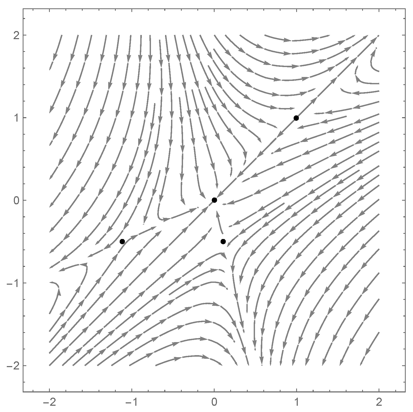
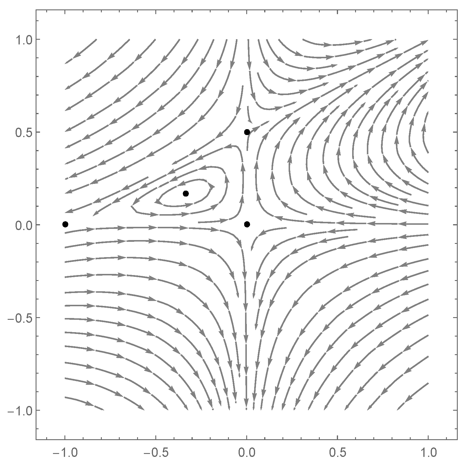
Example 1.

The vector of coefficients of the system

$$\begin{array}{ccc}\hfill \dot{x}& =\hfill & \hfill -x-2x^2+2xy+y^2\\ \hfill \dot{y}& =\hfill & \hfill -2x^2-y+4xy-y^2,\end{array}$$

(37)

see Figure 1, belongs to the variety $\mathbf{V}\left(I_{31}\right)$, so it is quite likely that there exists a linear transformation which brings this system to a ${\mathbb{Z}}_3$-equivariant one. After setting $\epsilon =1$, $q=3$ and $\rho =\sigma =0$ in equations $h_1=\dots =h_{16}=0$ and solving this system for $\alpha ,\beta ,\gamma ,\delta$, we get the solution

$$B=\left[\begin{array}{cc}\alpha & \beta \\ \gamma & \delta \end{array}\right]=\left[\begin{array}{cc}\frac{\sqrt{6}-1}{2}& -\frac{3}{2}\sqrt{\frac{3}{2}}\\ \sqrt{\frac{3}{2}}& \frac{-\sqrt{6}-1}{2}\end{array}\right],$$

which is not unique since the inverse of B is a generating symmetry as well. For finding the linear transformation S which will change the system in the ${\mathbb{Z}}_3$-equivariant one, we do the following. By the eigenvalue decomposition $R_3=S_R\mathrm{diag}(e^{2i\pi /3},e^{4i\pi /3})S_R^{-1}$ and $B=S_B\mathrm{diag}(e^{2i\pi /3},e^{4i\pi /3})S_B^{-1}$, we get $B=\left(S_B{S}_R^{-1}\right)R_3{\left(S_B{S}_R^{-1}\right)}^{-1}$. Therefore, the transformation matrix is

$$S=S_B{S}_R^{-1}=\left[\begin{array}{cc}\frac{\sqrt{2}}{2}& 1\\ 0& 1\end{array}\right].$$

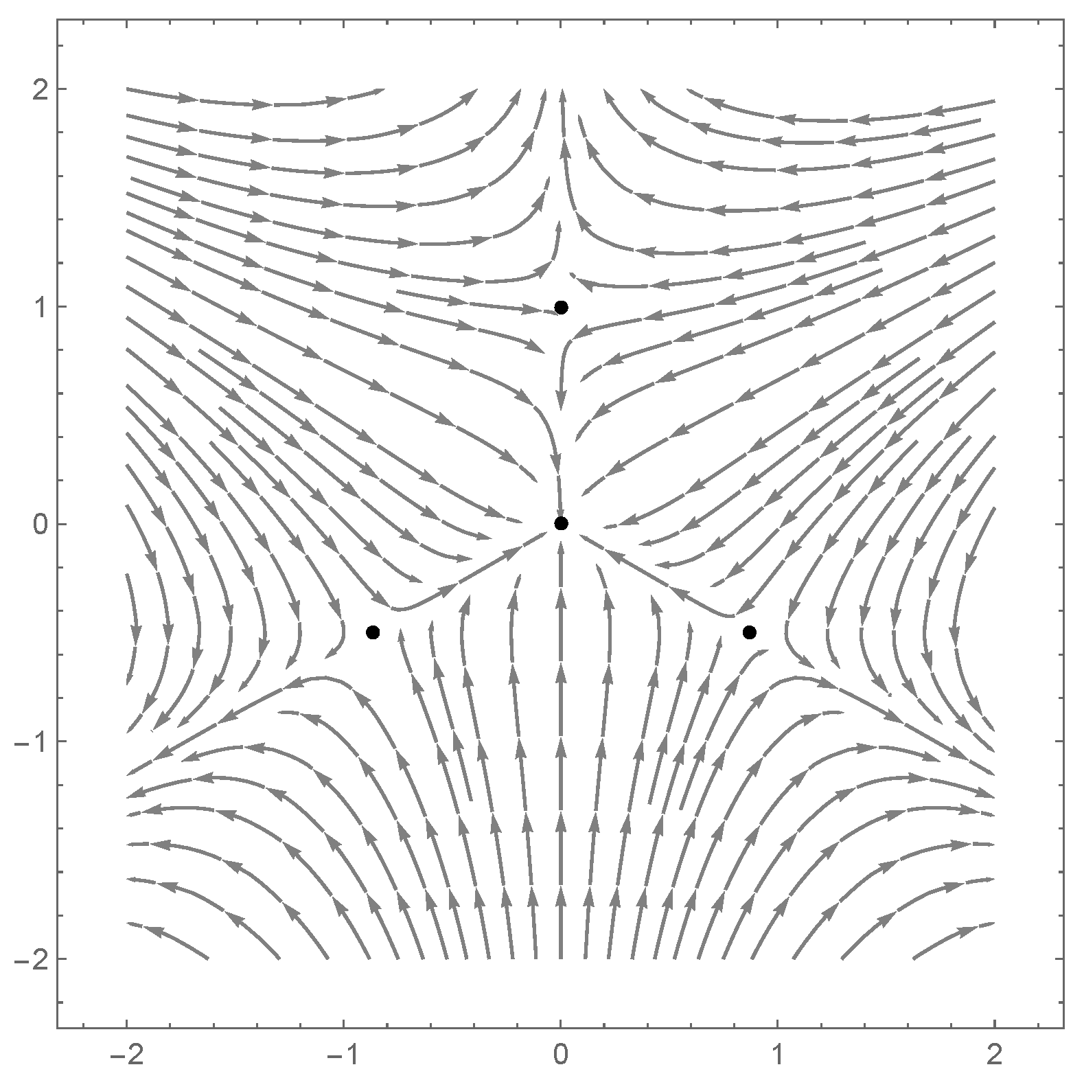
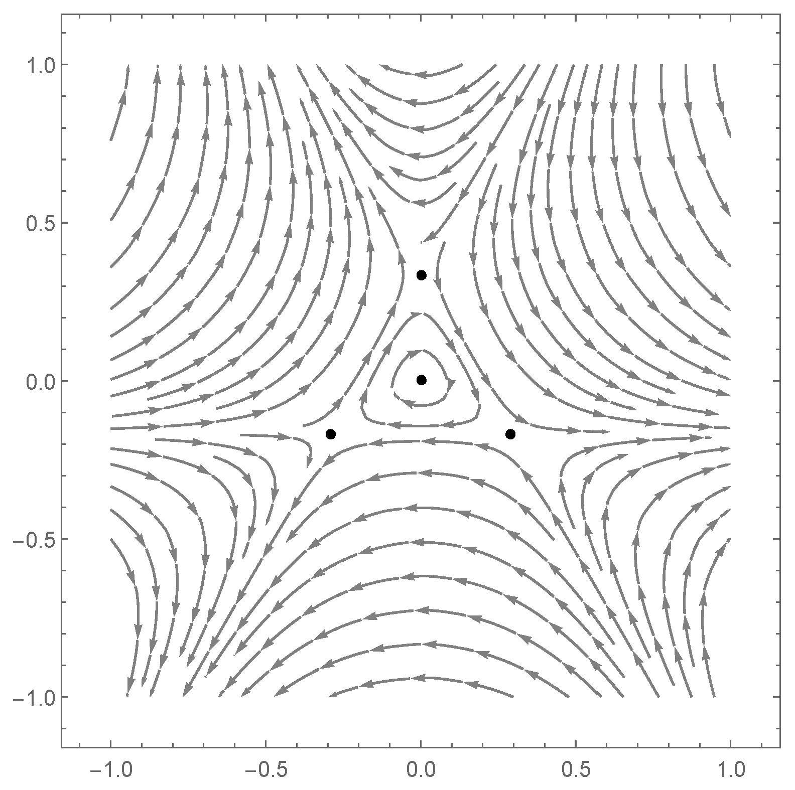
Now, the transformation $x=\frac{\sqrt{2}}{2}u+v$, $y=v$, converts the system to

$$\begin{array}{ccc}\hfill \dot{u}& =\hfill & \hfill -u-2uv\\ \hfill \dot{v}& =\hfill & \hfill -u^2-v+v^2,\end{array}$$

(38)

which is clearly $Z_3$-equivariant with a node at the origin, see Figure 2.

Example 2.

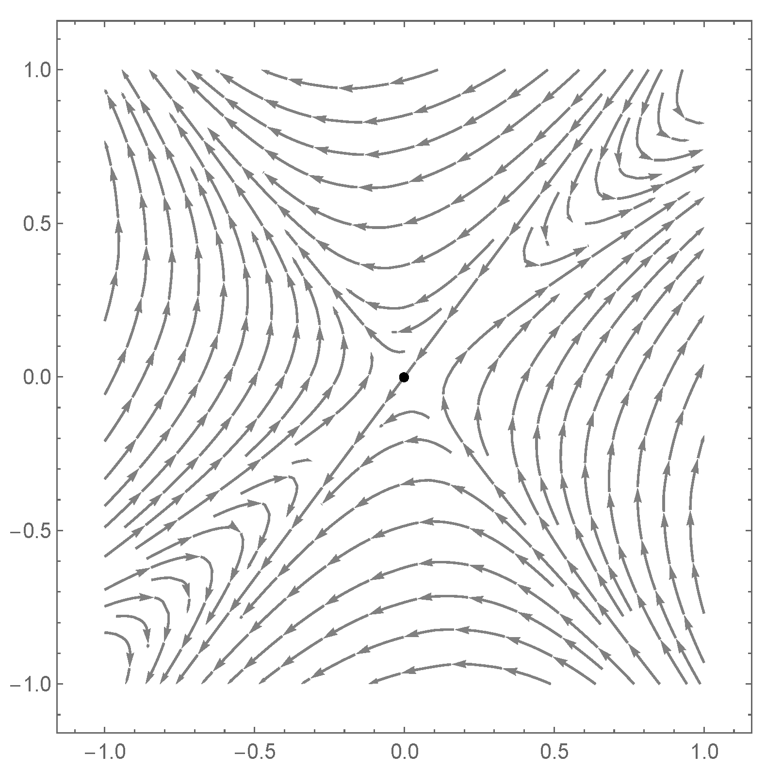
The next system will be one which we transform to a reversible $Z_6$-equivariant system by a bijective linear tranformation. We claim that the system below is a member of r${\mathcal{L}}_6$,

$$\begin{array}{ccc}\hfill \dot{x}& =\hfill & \hfill x^2+xy-2y^2\\ \hfill \dot{y}& =\hfill & \hfill 2x^2-2xy-y^2/2,\end{array}$$

(39)

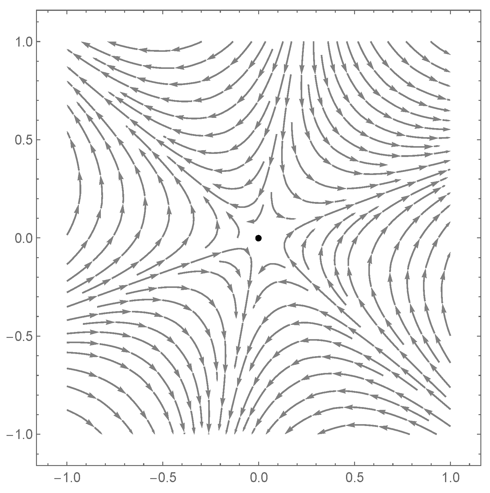
see Figure 3. Similarly as above, but this time taking ideal $I_6$ instead, we get the system

$$\begin{array}{ccc}\hfill \dot{u}& =\hfill & \hfill \frac{3}{32}\sqrt{23}{u}^2+\frac{23}{16}uv-\frac{3}{32}\sqrt{23}{v}^2\\ \hfill \dot{v}& =\hfill & \hfill \frac{23}{32}{u}^2-\frac{3}{16}\sqrt{23}uv-\frac{23}{32}{v}^2,\end{array}$$

(40)

see Figure 4. Moreover, we have the symmetry matrix

$$B=\left[\begin{array}{cc}\alpha & \beta \\ \gamma & \delta \end{array}\right]=\left[\begin{array}{cc}\frac{23-7\sqrt{69}}{46}& \frac{9\sqrt{69}}{46}\\ \frac{-4\sqrt{69}}{23}& \frac{23+7\sqrt{69}}{46}\end{array}\right],$$

and the linear transformation

$$S=\left[\begin{array}{cc}-\frac{\sqrt{23}}{8}& \frac{7}{8}\\ 0& 1\end{array}\right].$$

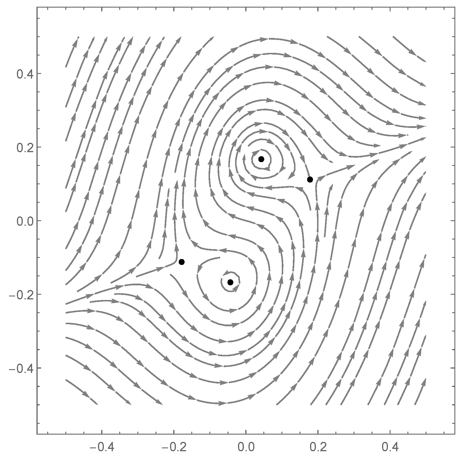
Example 3.

An example of system in ${\mathcal{A}}_3$ will be constructed so that we first fix the origin to be a saddle, then we choose a member $(\mathbf{a},\mathbf{b})\in \mathbf{V}\left(I_{32}\right)$ such that the corresponding system has four singular points. As above we find the matrix S representing the linear part of transformation and additionally the translation vector $(\rho ,\sigma )$. We start with

$$\begin{array}{ccc}\hfill \dot{x}& =\hfill & \hfill -x-x^2+4xy\\ \hfill \dot{y}& =\hfill & \hfill y+2xy-2y^2,\end{array}$$

(41)

see Figure 5, which parameter-vector belongs to $\mathbf{V}\left(I_{32}\right)$. The transformed system is now

$$\begin{array}{ccc}\hfill \dot{u}& =\hfill & \hfill v/\sqrt{3}+\sqrt{3}(u^2-v^2)\\ \hfill \dot{v}& =\hfill & \hfill -u/\sqrt{3}-2\sqrt{3}uv,\end{array}$$

(42)

see Figure 6, where the affine map $(x,y)=S(u,v)+(\rho ,\sigma )$ is defined by

$$S=\left[\begin{array}{cc}-\sqrt{3}& 1\\ 0& 1\end{array}\right],(\rho ,\sigma )=(-1/3,1/6).$$

We obtain exactly two solutions, the other one is the inverse map $(u,v)\mapsto S^{-1}(x,y)-S^{-1}(\rho ,\sigma )$.

Example 4.

Our last example presents a system which can be send to a reversible $Z_2$-equivariant one, here we actually need only translation because $R_2=-\mathrm{Id}$. Starting with the system

$$\begin{array}{ccc}\hfill \dot{x}& =\hfill & \hfill 2x^2-y-xy+\frac{25}{8}{y}^2\\ \hfill \dot{y}& =\hfill & \hfill x+4x^2-8xy+y^2,\end{array}$$

(43)

depicted in Figure 7, and transformed to

$$\begin{array}{ccc}\hfill \dot{u}& =\hfill & \hfill -\frac{1}{12}+2u^2-uv+\frac{25}{8}{v}^2\\ \hfill \dot{v}& =\hfill & \hfill \frac{1}{48}+4u^2-8uv+v^2,\end{array}$$

(44)

which phase portrait is drawn in Figure 8.

Note that this provides a simple method to construct a system with two singular points of the same kind.

References

- Romanovski, V.G. Time-reversibility in 2-dimensional systems. Open Syst. Inf. Dyn. 2008, 15, 359–370. [Google Scholar] [CrossRef]
- Han, M.; Petek, T.; Romanovski, V.G. Reversibility in polynomial sytems of ODE’s. Appl. Math. Comput. 2018, 338, 55–71. [Google Scholar]
- Lamb, J.S.W. Reversing Symmetries in dynamical systems. Physica A 1992, 25, 925–937. [Google Scholar] [CrossRef]
- Lamb, J.S.W.; Roberts, M. Reversible Equivariant systems. J. Differ. Equ. 1999, 159, 239–279. [Google Scholar] [CrossRef] [Green Version]
- Horn, R.A.; Johnson, C.R. Topics in Matrix Analysis; Cambridge University Press: Cambridge, UK, 1991. [Google Scholar]
- Li, J.; Zhao, X. Rotation symmetry groups of planar Hamiltonian systems. Ann. Differ. Equ. 1989, 5, 25–33. [Google Scholar]
- Han, M.; Sun, X. General form of Zq-reversible-equivariant planar systems and limit cycle bifurcations. J. Shanghai Norm. Univ. 2011, 40, 1–14. [Google Scholar]
- Cox, D.; Little, J.; O’Shea, D. Ideals, Varieties, and Algorithms: An Introduction to Computational Algebraic Geometry and Commutative Algebra; Springer: New York, NY, USA, 1997. [Google Scholar]
- Romanovski, V.G.; Shafer, D.S. The Center and Cyclicity Problems: A Computational Algebra Approach; Birkhauser: Boston, MA, USA, 2009. [Google Scholar]
- Decker, W.; Greuel, G.-M.; Pfister, G.; Shönemann, H. Singular 3-1-6–A Computer Algebra System for Polynomial Computations (2012). Available online: http://www.singular.uni-kl.de (accessed on 2 August 2020).
- Decker, W.; Laplagne, S.; Pfister, G.; Schonemann, H.A. primdec.lib. A Singular 3-1 Library for Computing the Prime Decomposition and Radical of Ideals. 2010. Available online: http://www.singular.uni-kl.de (accessed on 2 August 2020).
- Gianni, P.; Trager, B.; Zacharias, G. Gröbner bases and primary decomposition of polynomials. J. Symb. Comput. 1988, 6, 146–167. [Google Scholar] [CrossRef]
- Brjuno, A.D. Local Methods in Nonlinear Differential Equations; Springer: Berlin, Germany, 1989. [Google Scholar]
Figure 1.
System (37).
Figure 2.
System (38).
Figure 3.
System (39).
Figure 4.
System (40).
Figure 5.
System (41).
Figure 6.
System (42).
Figure 7.
System (43).
Figure 8.
System (44).
© 2020 by the authors. Licensee MDPI, Basel, Switzerland. This article is an open access article distributed under the terms and conditions of the Creative Commons Attribution (CC BY) license (http://creativecommons.org/licenses/by/4.0/).
Share and Cite
MDPI and ACS Style
Han, M.; Petek, T.; Romanovski, V.G. On Some Symmetries of Quadratic Systems. Symmetry 2020, 12, 1300. https://doi.org/10.3390/sym12081300
AMA Style
Han M, Petek T, Romanovski VG. On Some Symmetries of Quadratic Systems. Symmetry. 2020; 12(8):1300. https://doi.org/10.3390/sym12081300
Chicago/Turabian StyleHan, Maoan, Tatjana Petek, and Valery G. Romanovski. 2020. "On Some Symmetries of Quadratic Systems" Symmetry 12, no. 8: 1300. https://doi.org/10.3390/sym12081300
Note that from the first issue of 2016, this journal uses article numbers instead of page numbers. See further details here.