Towards a Hybrid Evaluation Approach to Chinese Sustainable Drinking Water Source Regions within an Uncertain Decision Environment

Abstract

Confronted with the increasingly serious water pollution in China, companies are implementing scientific measures to strive for sustainable drinking water source regions (DWSRs). The challenge lies in how to evaluate available DWSRs. Considering the complexity and uncertainty existing in the evaluation process, we deem this process a complicated multi-criteria group decision-making (MCGDM) problem. It involves fuzzy decision information, prioritized relationships among different criteria, and distinctively allocated weights of decision makers regarding different alternatives. By utilizing the asymmetrical weak probabilistic hesitant fuzzy elements (P-HFES) to depict fuzzy data, this paper leads a direction to investigating a data-driven MCGDM approach and its application to evaluate available DWSRs. First, considering the common sense that criteria are not always given symmetrical priority, we propose a series of aggregation operators for integrating weak P-HFEs by including the prioritized relationship of criteria. Moreover, the importance weights of criteria and decision makers are objectively determined through a priority-based basic unit interval and monotonic (P-BUM) function and some novel distance measures, respectively. Finally, an evaluation approach is established. It aims to handle MCGDM problems with incomplete weight information regarding the criteria and decision makers in weak probabilistic hesitant fuzzy circumstance. Practically, focusing on evaluating three DWSRs, a realistic example of application is furnished to verify the feasibility of the proposed approach.

1. Introduction

Along with the rapid development of the society, the problem of water pollution in China has become increasingly serious. Influenced by this phenomenon, the safety of drinking water is of great concern. Water source selection is one of the preventive measures to ensure the safety and hygiene of drinking water for residents [1]. Meanwhile, as China has become the largest consumer of bottled water, selecting an appropriate drinking water source region (DWSR) is also a challenge to companies when supporting the supply of drinks. Therefore, it is essential and practical to study how to select suitable DWSRs, which raises a complex decision-making problem that would always encounter uncertainty in an realistic decision environment. To address this issue, we concentrate on developing an evaluation approach for selecting available DWSRs from the angle of companies by answering several research questions:

(1)

Is it possible to accurately represent the contradictory evaluation results for DWSRs given by different decision makers?

(2)

As distinctive criteria are not equal and asymmetrically prioritized in terms of different decision makers’ preferences, how to generate weights of criteria?

(3)

How to distinguish different decision makers with respect to different alternatives?

(4)

How to fuse distinctive assessments of DWSRs without complaints, which may lead to the decline of decision efficiency?

Responding to these points, our research deals with multi-criteria group decision-making (MCGDM) problems defined in weak probabilistic hesitant fuzzy contexts and unknown weight information on the premise of an asymmetrical prioritization of criteria. The contributions of this study are:

(1) Information presentation. Differing from most MCGDM problems [2], the individual decision maker considered in this paper is not referred to an individual person, but an individual group. Actually, there are some available extensions of fuzzy sets that are capable of describing the decision information supplied by individual groups, such as probabilistic linguistic term sets [3] and picture fuzzy sets [4]. However, these sets are always defined to present complete information or are not able to show probabilistic information. Hence, considering the ability of weak probabilistic hesitant fuzzy elements (P-HFEs) for expressing distinctive opinions in a set and allowing incomplete probabilistic information, it is quite appropriate to use weak P-HFEs to express the opinions of each individual group.

(2) Weight generation function. In light of the asymmetrically prioritized relationship between criteria, we are going to extend the classical prioritized aggregation operators [5] to fuse criteria values regarding each alternative given by each group. Meanwhile, the prioritization given by each group will be utilized in a newly introduced priority-based basic unit interval and monotonic (P-BUM) function, to yield the importance weights of different criteria with respect to different alternatives.

(3) Information measurements. Commonly, large distance is in correspondence to little consensus [6,7]. Given that the numbers of the elements in different weak P-HFEs are not equal, this paper will introduce a series of Hausdorff distance measures to measure the distinction among different groups. Based on this, the weights of different groups under different alternatives will be generated.

(4) Information fusion. Generally speaking, aggregation operators are powerful tools to integrate the information derived from individuals in one group [8]. To synthesize distinctive opinions, a series of aggregation operators, which can be divided into two branches, will be developed. One branch contains two prioritized aggregation operators, aiming to fuse criteria values for alternatives. The other branch is to integrate group assessments by inserting the relationship between different groups into the extension of the classical induced ordered weighted averaging (IOWA) operator, which considers the special ability of an inducing variable.

(5) Approach development. A hybrid evaluation approach will be developed to handle an existing problem for evaluating DWSRs, which contains positive and negative decision information and incomplete weight information.

The rest of this paper is arranged as follows. In Section 2, a review of extant studies is presented. In Section 3, the weak P-HFEs with its operations and comparisons, as well as some aggregation operators are reviewed. Moreover, the innovative operators, which cover the previously defined two aggregation phases, are introduced. Moreover, a supported P-BUM function and a family of generalized Hausdorff distance measures are put forward. In Section 4, the background of the MCGDM problem being tackled in this paper and the corresponding solving approach are presented. In Section 5, an example of application regarding the evaluation for DWSRs is furnished. In Section 6, discussions including the findings of the experiment and comparisons are illustrated. In Section 7, conclusions are drawn.

2. Literature Review

Initiated by Zadeh [9], the fuzzy set is a powerful tool to represent uncertain information. During the last decades, it has been extended to various forms to accommodate complex and vague decision environments. These extended forms can be roughly captured by two branches: numeric and linguistic. Despite the success of a series improvement of the linguistic decision making [10,11,12,13], this has ignored the distortion of the original information because it usually requires some tools (the cloud model [14], linguistic scale function [15], the transformation function [16,17], etc.) to make the linguistic values calculable. Bearing this in mind, we intend to manage MCGDM problems with numeric values when there are uncertainties expressed by the weak P-HFEs, which can be deemed as an important extension of numeric fuzzy settings. Weak P-HFEs [18], including a hesitant fuzzy set [19] and corresponding probabilities, is a direct extension of the probabilistic hesitant fuzzy elements (P-HFEs) [20]. Despite the common advantage of these two sets for simultaneously representing positive and negative information, the weak P-HFEs further considered the incompleteness of probabilistic information. It is this idea that allows us to measure the degree of membership degree with its probabilities in realistic situations. Although there is some similar characteristics between weak P-HFSs and PHFSs, they differ from each other in the development of solving realistic problems. As to the PHFS, it has awakened high interest among the researchers [21,22,23], due to its ability to enrich the flexibility of expressing real-world decision information. Compared with the development of PHFSs and to the best of our knowledge, there is not a huge amount of literature reporting studies about the weak P-HFEs. This is possibly because the weak P-HFEs were newly introduced as a notable concept. To enhance and spread the applicability of weak P-HFEs, this paper will investigate MCGDM problems with weak probabilistic hesitant fuzzy information.

In general, the majority of selection issues contain fuzzy information and groups of decision makers, which are always addressed as MCGDM problems. Water source selection is an environmental process that is always concerned with the application of multi-criteria decision problems [24]. As a rule of thumb, when the decision makers involved in a decision process are no less than one, the multi-criteria decision converts to an MCGDM process. Furthermore, an MCGDM problem usually includes the fusion of decision information. For this, aggregation operators turn out to be an effective and powerful tool since they are so intuitive to fuse individual information by consideration of importance weights. Until now, a majority of distinctive aggregation operators are developed. Aiming to suit the MCGDM problem in this paper, the comprehensive assessments of each alternative as well as the overall opinions of all decision makers ought to be derived. As such, we define the fusion process into two phases, which are respectively in need of two types of aggregation operators:

(1) In terms of the synthesis of criteria values, we define the first fusion phase to be in accordance with the phenomenon of the prioritization between criteria, which appears frequently in real-life decision environments. To support this process, there are two fundamental issues to be solved: determining the weights and developing the operator. Nevertheless, early efforts in figuring out the incomplete weight information of criteria did not consider the prioritization relationship of criteria [25,26,27,28,29]. Oppositely, the prioritized average operators have absorbed not a few academic concentrations, including the prioritized aggregation operator [5], the prioritized ordered weighted averaging operator (POWA) [30], and their extensions [31,32,33,34]. Thus, the combination of the generation technique of objective weights for criteria and prioritized aggregation operators has some benefits in finding solutions to realistic decision-making problems.

(2) From the perspective of integrating individual opinions, we define the second fusion phase, which could reflect the relationship between individuals with respect to different alternatives. To accomplish this phase, a family of the IOWA operators [35] proves to be a suitable tool. This is because the necessary inducing variables could represent the relationship between argument variables. Following this idea, the extension of the IOWA operator to the weak probabilistic hesitant fuzzy environment poses a challenge as to how to determine the inducing variable. Undoubtedly, distance is a good choice. Measuring the distance between different objects is a useful way to manifest the relationship between them. To support this, the last decades have witnessed a lot of studies on different distance measures, such as the Hamming distance, the Euclidean distance, the Hausdorff distance, the Hybrid distance, the entropy-based distance, and the ordered weighted distance measure [28,36,37,38]. Except for the Hausdorff distance, the others all demand that the length of the compared objects should be the same. To some extent, this requirement may not be possible under a weak probabilistic hesitant fuzzy environment, due to the uncertainty expressed through the weak P-HFEs.

3. Related Works

This section firstly reviews some basic concepts related to the decision data in this paper. Furthermore, we discuss the extension of prioritized aggregation operators to weak probabilistic hesitant fuzzy environments. To complete the aggregation, a P-BUM function is established. Then, by considering the relationship between weak P-HFEs, we put forward a generalized aggregation operator, which is quantified by the introduction of a family of generalized Hausdorff distances.

3.1. Weak Probabilistic Hesitant Fuzzy Elements

Definition 1. [18]. Let $A$ be a fixed set. A weak P-HFE is defined in terms of a function that, when applied to $A$, returns to a subset of $[0,1]$ and is mathematically expressed as:

$$H=\left\{\langle a,h_a(p_a)\rangle |a\in A\right\},$$

(1)

where the values in both of the two sets $h_a$ and $p_a$ are lying in the range of $[0,1]$.

To be specific, the symbol $h_a$ refers to some possible membership degrees of $a\in A$ to the set $H$. Accordingly, $p_a$ stands for the associated possibilities with $h_a$.

For convenience, $h(p)=\left\{{\tau }_t(p_t)|t=1,2,\dots ,\#h(p)\right\}$ is called a weak P-HFE, in which ${\tau }_t(p_t)$ is defined as one of the $\#h$ terms in the weak P-HFE and ${\displaystyle {\sum }_{t=1}^{\#h(p)}{p}_t}\le 1$.

Definition 2. [18]. Let $h_l(p)=\left\{{\tau }_{t_l}(p_{t_l})|t_l=1,2,\dots ,\#h_l(p)\right\}(l=1,2)$ be two arbitrary weak P-HFEs and $\alpha >0$, then

(1) 

$\alpha h_l(p)={\displaystyle \underset{{\tau }_{t_l}\in h_l}{\cup }\left\{[1-{(1-{\tau }_{t_l})}^{\alpha }](p_{t_l})\right\}}$;

(2) 

${\left(h_l(p)\right)}^{\alpha }={\displaystyle \underset{{\tau }_{t_l}\in h_l}{\cup }{({\tau }_{t_l})}^{\alpha }(p_{t_l})\}}$;

(3) 

$h_1(p)\oplus h_2(p)={\displaystyle \underset{{\tau }_{t_l}\in h_l}{\cup }\left\{\left[{\tau }_{t_1}+{\tau }_{t_2}-{\tau }_{t_1}{\tau }_{t_2}\right]\left(\frac{p_{t_1}\cdot p_{t_2}}{{\displaystyle {\sum }_{t_1=1}^{\#h_1(p)}{p}_{t_1}}\cdot {\displaystyle {\sum }_{t_2=1}^{\#h_2(p)}{p}_{t_2}}}\right)\right\}}$; and

(4) 

$h_1(p)\otimes h_2(p)={\displaystyle \underset{{\tau }_{t_l}\in h_l}{\cup }\left\{\left[{\tau }_{t_1}{\tau }_{t_2}\right]\left(\frac{p_{t_1}\cdot p_{t_2}}{{\displaystyle {\sum }_{t_1=1}^{\#h_1(p)}{p}_{t_1}}\cdot {\displaystyle {\sum }_{t_2=1}^{\#h_2(p)}{p}_{t_2}}}\right)\right\}}$.

As to any fuzzy setting, comparison is imperative. In this paper, we adopt the following definition to compare any two weak P-HFEs.

Definition 3. [18] For a weak P-HFE $h(p)=\left\{{\tau }_t(p_t)|t=1,2,\dots ,\#h(p)\right\}$, its score and deviation degree are defined as:

$$\mu (h(p))=\frac{{\displaystyle {\sum }_{t=1}^{\#h(p)}{\tau }_t{p}_t}}{{\displaystyle {\sum }_{t=1}^{\#h(p)}{p}_t}},$$

(2)

$$\nu (h(p))=\frac{{\displaystyle {\sum }_{t=1}^{\#h(p)}{(p_t({\tau }_t-\mu ))}^2}}{{\displaystyle {\sum }_{t=1}^{\#h(p)}{p}_t}}.$$

(3)

Then, based on Equations (2) and (3), the comparison rules of two weak P-HFEs$h_l(p)=\left\{{\tau }_{t_l}(p_{t_l})|t_l=1,2,\dots ,\#h_l(p)\right\}(l=1,2)$can be summarized below.

(1) 

If$\mu (h_1(p))>\mu (h_2(p))$, then$h_1(p)>h_2(p)$;

(2) 

If$\mu (h_1(p))<\mu (h_2(p))$, then$h_1(p)<h_2(p)$;

(3) 

If$\mu (h_1(p))=\mu (h_2(p))$, then three situations exist:

1) 

If$\nu (h_1(p))>\nu (h_2(p))$, then$h_1(p)<h_2(p)$;

2) 

If$\nu (h_1(p))<\nu (h_2(p))$, then$h_1(p)>h_2(p)$;

3) 

If$\nu (h_1(p))=\nu (h_2(p))$, then$h_1(p)=h_2(p)$.

3.2. Prioritized Aggregation Operators

This subsection reviews some prioritized aggregation operators to facilitate further studies.

Definition 4. [5] Let $C=(c_1,c_2,\dots ,c_m)$ be a finite set of $m$ criteria. The prioritization of these criteria is mathematically predefined with a linear ordering $c_1\succ c_2\succ \cdots \succ c_m$, which implies that the priority of criterion $c_j$ becomes lower with the increase in the subscript of $c_j$. Assume $c_j(x)(c_j(x)\in [0,1])$ is the assessment value of an arbitrary alternative $x_i$ over $c_j$, then the prioritized average (PA) operator is defined with the following form:

$$PA(c_j(x))={\displaystyle {\sum }_{j=1}^m{w}_j}{c}_j(x),$$

(4)

where $w_j=\frac{u_j}{{\displaystyle {\sum }_{j=1}^m{u}_j}}$ with $u_j={\displaystyle {\prod }_{j^{\prime }=1}^{j-1}{c}_{j^{\prime }}(x)}$ and $u_1=1$.

To enforce the necessity of the prioritization between criteria, Yager [30] further put forward the POWA operator, which is originated from the idea of the normalized priority-based importance degrees and the BUM function [39].

Definition 5. [30]: Let $F$ be a BUM function and $\omega =({\omega }_1,{\omega }_2,\dots ,{\omega }_m)$ be the weight vector of criteria, then the POWA operator is mathematically defined as:

$$POWA(c_j(x))={\displaystyle {\sum }_{j=1}^m{\omega }_j{c}_{o(j)}(x)},$$

(5)

where the BUM function should satisfy $F:[0,1]\to [0,1]$, $F(0)=0$ and $F(1)=1$, and ${\omega }_j=F(w_{o(j)})-F(w_{o(j-1)})$, in which the value of $c_{o(j)}(x)$ ranks as the $j$th largest among $c_j(x)(j=1,2,\dots ,m)$.

3.3. Prioritized Weak Probabilistic Hesitant Fuzzy Weighted Averaging Operator

Motivated by the fundamental concepts of prioritized aggregation operators, this subsection introduces the prioritized weak probabilistic hesitant fuzzy weighted average (PWPHFWA) operator.

Definition 6.Let$C=(c_1,c_2,\dots ,c_m)$be a finite set of$m$criteria, which are partitioned by a prioritization$c_1\succ c_2\succ \cdots \succ c_m$, and assume$c_j(x)=\left\{{\tau }_{t_j}(p_{t_j})|t_j=1,2,\dots ,\#c_j(x)\right\}(l=1,2,\dots ,m)$is$m$weak P-HFEs representing the assessment value of an arbitrary alternative$x$over$c_j$. The PWPHFWA operator is an aggregation function with

$$PWPHFWA\left(c_j(x)\right)={\displaystyle {\sum }_{j=1}^m{w}_j}\cdot c_j(x),$$

(6)

where

$$w_j=\frac{s_j}{{\displaystyle {\sum }_{j=1}^m{s}_j}},$$

(7)

being

$$\{\begin{array}{l}{s}_1=1\\ s_j={\displaystyle {\prod }_{k=1}^{j-1}\frac{{\displaystyle {\sum }_{t_k=1}^{\#h_k(p)}{\tau }_{t_k}\cdot p_{t_k}}}{{\displaystyle {\sum }_{t_k=1}^{\#h_k(p)}{p}_{t_k}}}},for k=2,3,\dots ,m\end{array}.$$

(8)

Obviously, during the calculation of the weights of criteria, the probabilities are normalized and newly distributed. To some extent, this process avoids the ignorance of probabilistic information. In other words, this conforms to the habit of human beings that the sum of importance weights should be equal to 1.

To better understand the PWPHFWA operator, a practical example is illustrated below.

Example 1.Let the prioritized relationship of four criteria be$c_1\succ c_2\succ c_3\succ c_4$. Assume the criteria values for an alternative is$c_1(x)=\left\{0.6(0.4),0.7(0.3)\right\}$,$c_2(x)=\left\{0.4(0.2),0.5(0.5),0.6(0.1)\right\}$,$c_3(x)=\left\{0.8(0.7),0.9(0.3)\right\}$, and$c_4(x)=\left\{0.55(0.6),0.65(0.2)\right\}$.

As per Equation (8), we have $s_1=1$, $s_2=0.6429$, $s_3=0.3134$, and $s_4=0.2601$. Afterwards, from these results and according to Equation (7), we have $w_1=0.4512$, $w_2=2901$, $w_3=0.1414$, and $w_4=0.1173$. Then, utilizing Equation (6), one can obtain:

$$\begin{array}{ll}c(x)& =PWPHFWA\left(c_j(x)\right)\\ & ={\displaystyle {\sum }_{j=1}^4{w}_j\cdot c_j(x)}\\ & =\left\{\begin{array}{l}0.3386(0.4),\\ 0.4191(0.3)\end{array}\right\}\oplus \left\{\begin{array}{l}0.1377(0.2),\\ 0.2929(0.5),\\ 0.2334(0.1)\end{array}\right\}\oplus \left\{\begin{array}{l}0.2035(0.7),\\ 0.2779(0.3)\end{array}\right\}\oplus \left\{\begin{array}{l}0.0894(0.6),\\ 0.1159(0.2)\end{array}\right\}\\ & =\left\{\begin{array}{l}0.5864(0.075),0.5984(0.025),0.625(0.0322),0.6359(0.0107),0.6608(0.1875),\\ 0.6707(0.0625),0.6925(0.0803),0.7014(0.0268),0.6323(0.0375),0.6431(0.0125),\\ 0.6649(0.0161),0.6747(0.0053),0.6231(0.0563),0.6329(0.0187),0.6706(0.0241),\\ 0.6802(0.008),0.7021(0.1406),0.7107(0.0469),0.7092(0.0603),0.738(0.0201),\\ 0.677(0.0281),0.6864(0.0094),0.7072(0.0121),0.7157(0.004)\end{array}\right\}\end{array}$$

From this numeric example, the resulted criteria weights show their accordance with the predefined prioritization of criteria, and illustrate that the frontal prioritized criteria cannot be compensated by the posteriori ones.

Theorem 1.The aggregated value by the PWPHFWA operator is still a weak P-HFE.

It is obvious that this theorem always holds, so the proof is omitted here.

Theorem 2.The probabilistic information in the aggregated value by the PWPHFWA operator is completed, i.e., the sum of the associated probabilistic values equals to 1.

Proof. 

As per Equations (7)–(8), the original probabilistic information existing in each criterion value, which may not be coincident with human habits that the sum of the probabilistic values should be 1, is normalized by a division operation. Undoubtedly, this design firmly supports the establishment of Theorem 2.  □

Frankly speaking, the PWPHFWA operator does not possess the properties of idempotency, monotonicity and boundary. This conclusion can be drawn from an analysis that the addition between two identical weak P-HFEs would not result in the same value like other settings. Nevertheless, the commutative law of the PWPHFWA operator can be elucidated in the following theorem.

Theorem 3.

Let$C^{\prime }=({c^{\prime }}_1,{c^{\prime }}_2,\dots ,{c^{\prime }}_m)$be an arbitrary permutation of$C=(c_1,c_2,\dots ,c_m)$. Denote the prioritization of the permutated$m$criteria as${c^{\prime }}_{1^{\prime }}\succ {c^{\prime }}_{2^{\prime }}\succ \cdots \succ {c^{\prime }}_{m^{\prime }}$, where${c^{\prime }}_{j^{\prime }}(j=1,2,\dots ,m)$are, respectively, in the same position with$c_j(j=1,2,\dots ,m)$. Suppose${c^{\prime }}_j(x)=\left\{{{\tau }^{\prime }}_{t_j}({p^{\prime }}_{t_j})|t_j=1,2,\dots ,\#{c^{\prime }}_j(x)\right\}$$(l=1,2,\dots ,m)$are$m$weak P-HFEs representing the assessment value${c^{\prime }}_j$, then:

$$PWPHFWA\left(c_j(x)\right)=PWPHFWA\left({c^{\prime }}_j(x)\right),$$

(9)

where${c^{\prime }}_{j^{\prime }}(j=1,2,\dots ,m)$refer to the prioritized criteria of${c^{\prime }}_j(j=1,2,\dots ,m)$.

Remark. 

For the sake of the prioritized positions being predefined for every criterion, the new prioritization${c^{\prime }}_{1^{\prime }}\succ {c^{\prime }}_{2^{\prime }}\succ \cdots \succ {c^{\prime }}_{m^{\prime }}$totally equates to the original prioritization$c_1\succ c_2\succ \cdots \succ c_m$. In other words, whatever the permutation of the finite criteria is, the prioritization of the distinctive criteria is fixed.

Proof. 

Obviously, since the permutation does not influence the prioritized ranking of the criteria, the weight information of the permutated criteria is entirely the same as that of the original ranked criteria. Therefore, the aggregation results of $PWPHFWA\left(c_j(x)\right)$ and those of $PWPHFWA\left({c^{\prime }}_j(x)\right)$ would be the same. That is to say, Theorem 3 always holds. □

3.4. Prioritized Weak Probabilistic Hesitant Fuzzy Ordered Weighted Averaging Operator

To strengthen the power of the prioritization imperative, this subsection further proposes the prioritized weak probabilistic hesitant fuzzy ordered weighted averaging (PWPHFOWA) operator as follows.

Definition 7.

Let$F$be a BUM function and$C=(c_1,c_2,\dots ,c_m)$be a fixed set of$m$criteria with an associated prioritization$c_1\succ c_2\succ \cdots \succ c_m$. Suppose$c_j(x)=\left\{{\tau }_{t_j}(p_{t_j})|t_j=1,2,\dots ,\#c_j(x)\right\}$$(l=1,2,\dots ,m)$is$m$weak P-HFEs representing the assessment value of an arbitrary alternative$x$over$c_j$, then the PWPHFOWA operator is defined with the mathematical expression:

$$PWPHFOWA\left(c_j(x)\right)={\displaystyle {\sum }_{j=1}^m{\omega }_j}\cdot c_{o(j)}(x),$$

(10)

where the BUM function satisfies$F:[0,1]\to [0,1]$,$F(0)=0$and$F(1)=1$, and${\omega }_j=F(w_{o(j)})-F(w_{o(j-1)})$in which the value of$c_{o(j)}(x)$ranks as the$j$th largest among$c_j(x)(j=1,2,\dots ,m)$. In other words,$o:\{1,2,\dots ,m\}\to \{1,2,\dots ,m\}$is a permutation such that$c_{o(j)}(x)\ge c_{o(j+1)}(x)$, for$\forall j=1,2,\dots ,m-1$.

Theorem 4.

The aggregated value by the PWPHFOWA operator is still a weak P-HFE.

It is obvious that this theorem always holds, so the proof is omitted here.

Theorem 5.

The probabilistic information in the aggregated value by the PWPHFOWA operator is completed, i.e., the sum of the associated probabilistic values equals 1.

Similar to Theorem 2, this theorem can be easily proved.

Theorem 6.

Let$C^{\prime }=({c^{\prime }}_1,{c^{\prime }}_2,\dots ,{c^{\prime }}_m)$be an arbitrary permutation of$C=(c_1,c_2,\dots ,c_m)$. Denote the prioritization of the permutated$m$criteria as${c^{\prime }}_{1^{\prime }}\succ {c^{\prime }}_{2^{\prime }}\succ \cdots \succ {c^{\prime }}_{m^{\prime }}$, where${c^{\prime }}_{j^{\prime }}(j=1,2,\dots ,m)$are, respectively, in the same position with$c_j(j=1,2,\dots ,m)$. Assume${c^{\prime }}_j(x)=\left\{{{\tau }^{\prime }}_{t_j}({p^{\prime }}_{t_j})|t_j=1,2,\dots ,\#{c^{\prime }}_j(x)\right\}$$(l=1,2,\dots ,m)$is$m$weak P-HFEs representing the assessment value${c^{\prime }}_j$, then:

$$PWPHFOWA\left(c_j(x)\right)=PWPHFOWA\left({c^{\prime }}_j(x)\right),$$

(11)

where${c^{\prime }}_{j^{\prime }}(j=1,2,\dots ,m)$refer to the prioritized criteria of${c^{\prime }}_j(j=1,2,\dots ,m)$.

Proof. 

On one hand, from the definition of the PWPHFOWA operator, the reordered sequence of the criteria is determined by the original criteria values, so this variable would not be affected by the permutation of the criteria. On the other hand, the importance weights of the criteria are dependent on the BUM function and the normalized priority-based importance degrees derived from the priorities of the criteria. Clearly, this does not have any connection with the permutation of the criteria yet. Thereby, the proof of Theorem 6 is completed. □

In this PWPHFOWA operator, the sequence of the criteria weights is dominated by the weak P-HFEs expressing the criteria values for the alternative. Meanwhile, the normalized priority-based importance degrees generated from the prioritized information indirectly determines the weights of criteria by using a BUM function. Thereafter, there is a significant push towards the development of the BUM function, which should accommodate to the environment of prioritized weak probabilistic hesitant fuzzy information. Followed by the properties of the PWPHFOWA operator, we present a BUM function for weak P-HFEs as below.

Definition 8.

Let$H=\{h_1(p),h_2(p),\dots ,h_m(p)\}$be a collection of weak P-HFEs, and$\varphi =\{h_{o(1)},h_{o(2)},\dots ,h_{o(J)}\}(J\le m)$be a subset of$H$, then a P-BUM function is defined as:

$$\tilde{F}(\varphi )=\frac{{\displaystyle {\sum }_{j=1}^J{w}_{o(j)}}+J}{{\displaystyle {\sum }_{j=1}^n{w}_j}+m},$$

(12)

where$w_{o(j)}$is the corresponding importance degree of the criterion value, which is ranked as the$j$th position with a decreasing sequence.

Theorem 7.

For the P-BUM function, it has the following properties:

(1) 

Boundary: For$\varphi \subset H$,$\tilde{F}(\varphi )\in [0,1]$, especially for an empty set$\vartheta$, i.e., no element is included in$\vartheta$,$\tilde{F}(\vartheta )=0$. On the contrary, for a universal set$H$,$\tilde{F}(H)=1$.

(2) 

Monotonicity: If${\varphi }_1\subset {\varphi }_2\subset H$, then$\tilde{F}({\varphi }_1)\le \tilde{F}({\varphi }_2)$.

It is obvious that these two properties naturally hold. Thereby, we omit the proof here.

Example 2.

Assume the criterion values for an alternative is$c_1(x)=\left\{0.6(0.4),0.7(0.3)\right\}$,$c_2(x)=\left\{0.4(0.2),0.5(0.5),0.6(0.1)\right\}$,$c_3(x)=\left\{0.8(0.7),0.9(0.3)\right\}$, and$c_4(x)=\left\{0.55(0.6),0.65(0.2)\right\}$. The prioritized relationship between these four criteria is$c_1\succ c_2\succ c_3\succ c_4$.

First of all, rank the criteria values by employing Definition 3. The scores and the ranking are listed as follows:

$${\mu }_1(x)=0.6429,{\mu }_2(x)=0.4125,{\mu }_3(x)=0.83,{\mu }_4(x)=0.575.$$

From the scores, one can easily discriminate the orders of the four criteria as $c_3(x)>c_1(x)>c_4(x)>c_2(x)$. Following this, the criteria are reordered as:

$$\begin{array}{l}{c}_{o(1)}(x)=c_3(x)=\left\{0.8(0.7),0.9(0.3)\right\},c_{o(2)}(x)=c_1(x)=\left\{0.6(0.4),0.7(0.3)\right\},\\ c_{o(3)}(x)=c_4(x)=\left\{0.55(0.6),0.65(0.2)\right\},c_{o(4)}(x)=c_2(x)=\left\{0.4(0.2),0.5(0.5),0.6(0.1)\right\}.\end{array}$$

Correspondingly, by taking advantage of the results in Example 1, we have the criteria satisfactions numerically expressed by the normalized priority-based importance degrees are newly endowed with

$$w_{o(1)}=w_3=0.1414,w_{o(2)}=w_1=0.4512,w_{o(3)}=w_4=0.1173,w_{o(4)}=w_2=2901.$$

Then, utilizing the P-BUM function, one can obtain the weight information related to the criteria as:

$\begin{array}{l}{\omega }_1=\tilde{F}(w_{o(1)})-\tilde{F}(\vartheta )=\frac{0.1414+1}{{\displaystyle {\sum }_{j=1}^4{w}_j}+4}-0=0.2283,\\ {\omega }_2=\tilde{F}(w_{o(2)})-\tilde{F}(w_{o(1)})=\frac{0.1414+0.4512+2}{{\displaystyle {\sum }_{j=1}^4{w}_j}+4}-\frac{0.1414+1}{{\displaystyle {\sum }_{j=1}^4{w}_j}+4}=0.2902,\\ {\omega }_3=\tilde{F}(w_{o(3)})-\tilde{F}(w_{o(2)})=\frac{0.1414+0.4512+0.1173+3}{{\displaystyle {\sum }_{j=1}^4{w}_j}+4}-\frac{0.1414+0.4512+2}{{\displaystyle {\sum }_{j=1}^4{w}_j}+4}=0.2235,\\ {\omega }_4=\tilde{F}(w_{o(4)})-\tilde{F}(w_{o(3)})=1-\frac{0.1414+0.4512+0.1173+3}{{\displaystyle {\sum }_{j=1}^4{w}_j}+4}=0.258.\end{array}$ Finally, By employing Equation (10), we have the comprehensive value of alternative $x$ as:

$$\begin{array}{ll}c(x)& =PWPHFOWA\left(c_j(x)\right)\\ & ={\displaystyle {\sum }_{j=1}^m{\omega }_j}\cdot c_{o(j)}(x)\\ & ={\omega }_1\cdot c_3(x)\oplus {\omega }_2\cdot c_1(x)\oplus {\omega }_3\cdot c_4(x)\oplus {\omega }_4\cdot c_2(x)\\ & =\left\{\begin{array}{l}0.6107(0.075),0.6286(0.1875),0.6494(0.0375),0.632(0.025),0.649(0.0625),\\ 0.6686(0.0125),0.6419(0.0563),0.6584(0.1406),0.7246(0.0281),0.6615(0.0188),\\ 0.6771(0.0469),0.6951(0.0093),0.6677(0.0322),0.683(0.0804),0.7007(0.016),\\ 0.6859(0.0107),0.7003(0.0268),0.717(0.0053),0.6943(0.0241),0.7083(0.0603),\\ 0.7246(0.0121),0.711(0.008),0.7243(0.02),0.7397(0.0041)\end{array}\right\}\end{array}$$

3.5. Weak Probabilistic Hesitant Fuzzy Induced Ordered Weighted Averaging Operators

The above presented PWPHFOWA operator is an extension of the POWA operator under a weak probabilistic hesitant fuzzy environment. If we take the prioritized information as an inducing variable, this POWA operator may be deemed as a special case of the IOWA operator [35]. Bearing this in mind, this subsection aims to present a more general type of the PWPHFOWA operator. In detail, the weak probabilistic hesitant fuzzy IOWA (WPHFIOWA) operator, together with its properties, is going to be studied.

Definition 9.

Let$H=\left(h_1(p),h_2(p),\dots ,h_L(p)\right)$be a collection of weak P-HFEs. A WPHFIOWA operator of dimension$m$is an aggregation function with the following expression:

$$WPHFIOWA\left(\langle {\sigma }_1,h_1(p)\rangle ,\langle {\sigma }_2,h_2(p)\rangle ,\dots ,\langle {\sigma }_L,h_L(p)\rangle \right)={\displaystyle {\sum }_{l=1}^L{v}_{o(l)}\cdot h_{o(l)}(p)},$$

(13)

where${\sigma }_l$plays the part of the inducing variable and$h_l(p)$is called the argument variable. Moreover, according to the ranking of the inducing variables$\left({\sigma }_1,{\sigma }_2,\dots ,{\sigma }_L\right)$,$\left(h_1(p),h_2(p),\dots ,h_l(p)\right)$is reordered and denoted by$\left(h_{o(1)}(p),h_{o(2)}(p),\dots ,h_{o(L)}(p)\right)$.

In Equation (13), based on the value of ${\sigma }_l$ and a quantifier guided function [39], the weight information $v_{o(l)}$ could be indirectly decided. In what follows, some properties of this WPHFIOWA operator are studied.

Theorem 8.

The aggregated value by the WPHFIOWA operator is still a weak P-HFE.

It is obvious that this theorem always holds, so the proof is omitted here.

Theorem 9.

The probabilistic information in the aggregated value by the WPHFIOWA operator is completed, i.e., the sum of the associated probabilistic values equals to 1.

Similar to Theorem 2, this theorem can be easily proved.

Theorem 10.

Let$H^{\prime }=\left({h^{\prime }}_1(p),{h^{\prime }}_2(p),\dots ,{h^{\prime }}_L(p)\right)$be any permutation of$H=\left(h_1(p),h_2(p),\dots ,h_L(p)\right)$, then:

$$\begin{array}{l}WPHFIOWA\left(\langle {\sigma }_1,h_1(p)\rangle ,\langle {\sigma }_2,h_2(p)\rangle ,\dots ,\langle {\sigma }_L,h_L(p)\rangle \right)\\ \hspace{1em}\hspace{1em}=WPHFIOWA\left(\langle {{\sigma }^{\prime }}_1,{h^{\prime }}_1(p)\rangle ,\langle {{\sigma }^{\prime }}_2,{h^{\prime }}_2(p)\rangle ,\dots ,\langle {{\sigma }^{\prime }}_L,{h^{\prime }}_L(p)\rangle \right)\end{array}$$

where${{\sigma }^{\prime }}_l(l=1,2,\dots ,L)$are the associating inducing variables of${h^{\prime }}_l(p)(l=1,2,\dots ,L)$.

This theorem can be analogously verified by reference to the proof of Theorem 6.

As is well known, central to the IOWA operator is the implementation of the inducing variable, which is a deterministic factor in the aggregation process. Generally, many indices can be applied to undertake this role for formulating the relationship between the argument variables. For the sake that the distance between two objects could intuitively reflect their distinction, we consider the distances between weak P-HFEs to be inducing variables.

Definition 10.

Let$h_l(p)=\left\{{\tau }_{t_l}(p_{t_l})|t_l=1,2,\dots ,\#h_l(p)\right\}(l=1,2)$be two arbitrary weak P-HFEs, the generalized Hausdorff distance measure between$h_1(p)$and$h_2(p)$can be mathematically defined with the following form:

$$D_{gH}\left(h_1(p),h_2(p)\right)={\left\{\frac{1}{2}\left[\begin{array}{l}\frac{1}{\#h_1(p)}{\displaystyle {\sum }_{t_1=1}^{\#h_1(p)}\underset{{\tau }_{t_2}(p_{t_2})\in h_2(p)}{\min }{\left(\left|\frac{{\tau }_{t_1}{p}_{t_1}}{{\displaystyle {\sum }_{t_1=1}^{\#h_1(p)}{p}_{t_1}}}-\frac{{\tau }_{t_2}{p}_{t_2}}{{\displaystyle {\sum }_{t_2=1}^{\#h_2(p)}{p}_{t_2}}}\right|\right)}^{\lambda }}+\\ \frac{1}{\#h_2(p)}{\displaystyle {\sum }_{t_2=1}^{\#h_2(p)}\underset{{\tau }_{t_1}(p_{t_1})\in h_1(p)}{\min }{\left(\left|\frac{{\tau }_{t_2}{p}_{t_2}}{{\displaystyle {\sum }_{t_2=1}^{\#h_2(p)}{p}_{t_2}}}-\frac{{\tau }_{t_1}{p}_{t_1}}{{\displaystyle {\sum }_{t_1=1}^{\#h_1(p)}{p}_{t_1}}}\right|\right)}^{\lambda }}\end{array}\right]\right\}}^{\frac{1}{\lambda }},$$

(14)

where$\lambda >0$.

This distance measure satisfies some properties summarized below.

Theorem 11.

Let$h_l(p)=\left\{{\tau }_{t_l}(p_{t_l})|t_l=1,2,\dots ,\#h_l(p)\right\}(l=1,2,3)$be any three weak P-HFEs, then

(1) 

$D_{gH}\left(h_1(p),h_2(p)\right)\ge 0$;

(2) 

$D_{gH}\left(h_1(p),h_2(p)\right)=0$, iff$h_1(p)=h_2(p)$;

(3) 

$D_{gH}\left(h_1(p),h_2(p)\right)=D_{gH}\left(h_2(p),h_1(p)\right)$; and

(4) 

If$h_1(p)<h_2(p)<h_3(p)$, then$D_{gH}\left(h_2(p),h_3(p)\right)\le D_{gH}\left(h_1(p),h_3(p)\right)$and$D_{gH}\left(h_1(p),h_2(p)\right)\le D_{gH}\left(h_1(p),h_3(p)\right)$.

It is obvious that properties (1–3) naturally hold. Herein, we just provide the proof process of the last property in Theorem 11 in the Appendix.

In the following, we take an analysis of the WPHFIOWA operator by configuring the value of the parameter $\lambda$.

If $\lambda =1$, then the above generalized Hausdorff distance measure degenerates to the following Hamming–Hausdorff distance measure between $h_1(p)$ and $h_2(p)$:

$$D_{HH}\left(h_1(p),h_2(p)\right)=\frac{1}{2}\left[\begin{array}{l}\frac{1}{\#h_1(p)}{\displaystyle {\sum }_{t_1=1}^{\#h_1(p)}\underset{{\tau }_{t_2}(p_{t_2})\in h_2(p)}{\min }\left(\left|\frac{{\tau }_{t_1}{p}_{t_1}}{{\displaystyle {\sum }_{t_1=1}^{\#h_1(p)}{p}_{t_1}}}-\frac{{\tau }_{t_2}{p}_{t_2}}{{\displaystyle {\sum }_{t_2=1}^{\#h_2(p)}{p}_{t_2}}}\right|\right)}+\\ \frac{1}{\#h_2(p)}{\displaystyle {\sum }_{t_2=1}^{\#h_2(p)}\underset{{\tau }_{t_1}(p_{t_1})\in h_1(p)}{\min }\left(\left|\frac{{\tau }_{t_2}{p}_{t_2}}{{\displaystyle {\sum }_{t_2=1}^{\#h_2(p)}{p}_{t_2}}}-\frac{{\tau }_{t_1}{p}_{t_1}}{{\displaystyle {\sum }_{t_1=1}^{\#h_1(p)}{p}_{t_1}}}\right|\right)}\end{array}\right].$$

(15)

If $\lambda =2$, then the above generalized Hausdorff distance measure degenerates to the following Euclidean–Hausdorff distance measure:

$$D_{EH}\left(h_1(p),h_2(p)\right)={\left\{\frac{1}{2}\left[\begin{array}{l}\frac{1}{\#h_1(p)}{\displaystyle {\sum }_{t_1=1}^{\#h_1(p)}\underset{{\tau }_{t_2}(p_{t_2})\in h_2(p)}{\min }{\left(\left|\frac{{\tau }_{t_1}{p}_{t_1}}{{\displaystyle {\sum }_{t_1=1}^{\#h_1(p)}{p}_{t_1}}}-\frac{{\tau }_{t_2}{p}_{t_2}}{{\displaystyle {\sum }_{t_2=1}^{\#h_2(p)}{p}_{t_2}}}\right|\right)}^2}+\\ \frac{1}{\#h_2(p)}{\displaystyle {\sum }_{t_2=1}^{\#h_2(p)}\underset{{\tau }_{t_1}(p_{t_1})\in h_1(p)}{\min }{\left(\left|\frac{{\tau }_{t_2}{p}_{t_2}}{{\displaystyle {\sum }_{t_2=1}^{\#h_2(p)}{p}_{t_2}}}-\frac{{\tau }_{t_1}{p}_{t_1}}{{\displaystyle {\sum }_{t_1=1}^{\#h_1(p)}{p}_{t_1}}}\right|\right)}^2}\end{array}\right]\right\}}^{\frac{1}{2}}.$$

(16)

By taking the distance between two weak P-HFEs as the inducing variable, we can characterize an extension of the IOWA operator defined below.

Definition 11.

Let$H=\left(h_1(p),h_2(p),\dots ,h_L(p)\right)$be a collection of weak P-HFEs, a weak probabilistic hesitant fuzzy distance-based IOWA (WPHFD-IOWA) operator of dimension$m$is an aggregation function mathematically defined as:

$$WPHFD-IOWA\left(\langle D_1,h_1(p)\rangle ,\langle D_2,h_2(p)\rangle ,\dots ,\langle D_L,h_L(p)\rangle \right)={\displaystyle {\sum }_{l=1}^L{v}_{o(l)}\cdot h_{o(l)}(p)}$$

(17)

where$D_l=\frac{{\displaystyle {\sum }_{l^{\prime }=1,l^{\prime }\ne l}^L{D}_{gH}\left(h_l(p),h_{l^{\prime }}(p)\right)}}{L-1}$and$v_{o(l)}=\frac{1-D_{o(l)}}{{\displaystyle {\sum }_{l=1}^L(1-D_l)}}$with$v_l\in [0,1]$and${\displaystyle {\sum }_{l=1}^L{\nu }_L}=1$. Definitely,$D_l$stands for the distance of$h_l(p)$to others and$D_{o(l)}$denotes the$l$th smallest one among$D_l(l=1,2,\dots ,L)$.

Similarly, this WPHFD-IOWA operator possesses the same properties with the WPHFIOWA operator. Such properties are introduced by Theorems 8–10.

4. Methodology

This section firstly formulates a group decision environment on the basis of weak P-HFEs. Within this fuzzy environment, an evaluation method for handling MCGDM problems, where the criteria are given a prioritization relationship and the weight information is unknown, is proposed.

4.1. Problem Statement

Consider the kind of MCGDM problems within an uncertain decision environment involving the weak probabilistic hesitant fuzzy information. Suppose $X=\{x_1,x_2,\dots ,x_n\}$ is the alternative set, in which $n$ indicates the number of alternatives. Define $C=(c_1,c_2,\dots ,c_m)$ as a finite set of $m$ criteria, for which the importance information is unknown. Besides, these criteria are not given symmetrical priority, due to the subjective distinction of decision makers. Let $G=\{g^1,g^2,\dots ,g^q\}$ denote $q$ groups of decision makers who are invited to furnish their opinions of alternatives with respect to different criteria. The opinion of group $g^d(d=1,2,\dots ,q)$ for alternative $x_i(i=1,2,\dots ,n)$ with respect to criteria $c_j(j=1,2,\dots ,m)$ is performed by a weak P-HFE denoted as $h_{ij}^d(p)=\left\{{\tau }_{t_{ij}^d}(p_{t_{ij}^d})|t_{ij}^d=1,2,\dots ,\#h_{ij}^d(p)\right\}$. Overall, the evaluation ratings of alternatives are characterized by $q$, and weak probabilistic hesitant fuzzy decision matrices are represented by $R^d={(r_{ij}^d)}_{n\times m}={\left(h_{ij}^d(p)\right)}_{n\times m}(d=1,2,\dots ,q)$. Except for providing judgments on alternatives, each group is required to provide a prioritization of the criteria with a linear ordering $c_{d_1}\succ c_{d_2}\succ \cdots \succ c_{d_m}$, in which $c_{d_j}$ implies the priority of criterion $c_j$ given by group $g^d$.

4.2. Approach to MCGDM under Weak Probabilistic Hesitant Fuzzy Environment

Based on the previously proposed operators and distances, this subsection develops an evaluation approach to address MCGDM problems, where the criteria values are represented by weak probabilistic hesitant fuzzy decision matrices. Besides, the related weight information is missing.

Step 1. Collect the decision information given by different groups of decision makers and construct the corresponding weak probabilistic hesitant fuzzy decision matrices as $R^d(d=1,2,\dots ,q)$.

Step 2. Apply the following functions, which are related to the PWPHFWA operator, to generate the normalized priority-based importance degrees related to different groups from the prioritized information.

$$\{\begin{array}{l}{s}_1^d=1\\ s_j^d={\displaystyle {\prod }_{k=1}^{j-1}\frac{{\displaystyle {\sum }_{t_{ik}^d=1}^{\#h_{ik}^d(p)}{\tau }_{t_{ik}^d}\cdot p_{t_{ik}^d}}}{{\displaystyle {\sum }_{t_{ik}^d=1}^{\#h_{ik}^d(p)}{p}_{t_{ik}^d}}}},forj=2,3,\dots ,m\end{array},$$

(18)

$$w_j^d=\frac{s_j^d}{{\displaystyle {\sum }_{j=1}^m{s}_j^d}}.$$

(19)

Step 3. By referring to Definition 3, rank the criteria values related to different alternatives and distinctive groups, and then match the weights with the reordered criteria.

Step 4. Determine the importance weights of criteria regarding different alternatives and distinctive groups by operating the P-BUM function. That is,

$$\tilde{F}(w_{o(j)}^d)=\frac{{\displaystyle {\sum }_{j=1}^J{w}_{o(j)}^d}+J}{{\displaystyle {\sum }_{j=1}^n{w}_j^d}+m},$$

(20)

$${\omega }_j^d=\tilde{F}(w_{o(j)}^d)-\tilde{F}(w_{o(j-1)}^d),$$

(21)

where $w_{o(j)}^d$ is defined as the corresponding importance degree of the criterion, which is ranked as the $j$th position under a decreasing sequence.

Step 5. Employ the PWPHFOWA operator to obtain the comprehensive criteria values for different groups $R_{\mathrm{C}}^d={\left(h_1^d(p),h_2^d(p),\dots ,h_n^d(p)\right)}^T$ with $h_i^d(p)=\left\{{\tau }_{t_i^d}(p_{t_i^d})|t_i^d=1,2,\dots ,\#h_i^d(p)\right\}$$(i=1,2,\dots ,n)$. That is,

$$PWPHFOWA\left(h_{ij}^d(p)\right)={\displaystyle {\sum }_{j=1}^m{\omega }_j^d}\cdot h_{io(j)}^d(p),$$

(22)

where $o:\{1,2,\dots ,m\}\to \{1,2,\dots ,m\}$ is a permutation such that $h_{io(j)}^d(p)\ge h_{io(j+1)}^d(p)$, for $\forall j=1,2,\dots ,m-1$.

After this manipulation, the results related to each group contain $n$ values, which represent the group assessment over $n$ alternatives.

Step 6. Taking the ease of employment and computational efficiency into consideration, we utilized the Hamming–Hausdorff distance measure to calculate the distances between one group and another one with respect to different alternatives. That is,

$$D_{HH}\left(h_i^d(p),h_i^{d^{\prime }}(p)\right)=\frac{1}{2}\left[\begin{array}{l}\frac{1}{\#h_i^d(p)}{\displaystyle {\sum }_{t_i^d=1}^{\#h_i^d(p)}\underset{{\tau }_{t_i^{d^{\prime }}}\left(p_{t_i^{d^{\prime }}}\right)\in h_i^{d^{\prime }}(p)}{\min }\left(\left|\frac{{\tau }_{t_i^d}{p}_{t_i^d}}{{\displaystyle {\sum }_{t_i^d=1}^{\#h_i^d(p)}{p}_{t_i^d}}}-\frac{{\tau }_{t_i^{d^{\prime }}}{p}_{t_i^{d^{\prime }}}}{{\displaystyle {\sum }_{t_i^{d^{\prime }}=1}^{\#h_i^{d^{\prime }}(p)}{p}_{t_i^{d^{\prime }}}}}\right|\right)}+\\ \frac{1}{\#h_i^{d^{\prime }}(p)}{\displaystyle {\sum }_{t_i^{d^{\prime }}=1}^{\#h_i^{d^{\prime }}(p)}\underset{{\tau }_{t_i^d}\left(p_{t_i^d}\right)\in h_i^d(p)}{\min }\left(\left|\frac{{\tau }_{t_i^{d^{\prime }}}{p}_{t_i^{d^{\prime }}}}{{\displaystyle {\sum }_{t_i^{d^{\prime }}=1}^{\#h_i^{d^{\prime }}(p)}{p}_{t_i^{d^{\prime }}}}}-\frac{{\tau }_{t_i^d}{p}_{t_i^d}}{{\displaystyle {\sum }_{t_i^d=1}^{\#h_i^d(p)}{p}_{t_i^d}}}\right|\right)}\end{array}\right],$$

(23)

where $d^{\prime }=1,2,\dots ,n$ with $d^{\prime }\ne d$.

Step 7. Distinguish the distinction of one group with others with respect to different alternatives by calculating the average distance of one group to all the others with

$$D_{HH}\left(g_i^d\right)=\frac{{\displaystyle {\sum }_{d^{\prime }=1,d^{\prime }\ne d}^q{D}_{HH}\left(h_i^d(p),h_i^{d^{\prime }}(p)\right)}}{q-1}.$$

(24)

Step 8. Compute the weights of different groups relating to different alternatives by

$$v_i^{o(d)}=\frac{1-D_{HH}\left(g_i^{o(d)}\right)}{{\displaystyle {\sum }_{d=1}^q\left(1-D_{HH}\left(g_i^d\right)\right)}}.$$

(25)

where $o:\{1,2,\dots ,q\}\to \{1,2,\dots ,q\}$ is a permutation such that $D_{HH}\left(g_i^{o(d)}\right)\le D_{HH}\left(g_i^{o(d+1)}\right)$.

In some cases, there may exist the situation where a group rather prefers one alternative that their judgments may be far away from those of other groups, such that these judgments cannot be importantly weighted. Occasionally, this is common in real-life decision-making processes. In this situation, regarding one alternative, the distance value of this group to others may be very small such that the opinions of this group should not be greatly taken into consideration. Nevertheless, this disparity can be offset by the distances of this group to others in view of the other alternatives. Bearing this in mind, we consider the weights of different groups with respect to different alternatives, respectively. Therefore, the operation in this step does not allow for compensation between distances, i.e., the phenomenon that the far distance representing the poor relationship of the group to others would not reduce the ability of better relationship for compensation by poorer ones. Based on this, the weight generation process of different groups remains impartial.

Step 9. Fuse the opinions of different groups by utilizing the WPHFD-IOWA operator, i.e.,

$$WPHFD-IOWA\left(\begin{array}{l}\langle D_{HH}\left(g_i^1\right),h_i^1(p)\rangle ,\langle D_{HH}\left(g_i^2\right),h_i^2(p)\rangle ,\dots ,\\ \langle D_{HH}\left(g_i^q\right),h_i^q(p)\rangle \end{array}\right)={\displaystyle {\sum }_{d=1}^q{v}_i^{o(d)}\cdot h_i^{o(d)}(p)}.$$

(26)

By this step, the overall assessment for each alternative can be obtained.

Step 10. According to Definition 3, assess the alternatives by listing rankings of them.

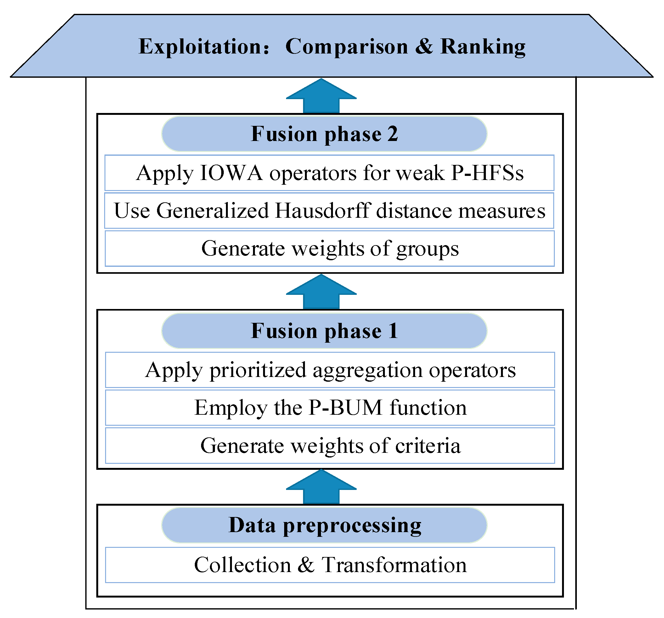
The innovations contained in this approach are graphically described in Figure 1.

5. Application and Results

This section concentrates on applying the evaluation approach to a practical problem concerning the assessment of sustainable drinking water source regions for a company in Singapore.

5.1. Problem Statement

Being a young company located in Singapore, Bello Group Pte. Ltd. commits to the research and development, production and sales of high-end differentiated beverages. Until now, its business has spread in various countries, such as China, Singapore, Indonesia, Malaysia, Cambodia, Vietnam, Maldives, and the United States. However, faced with the increasingly serious water pollution, how to evaluate and select sustainable drinking water source region(s) poses a challenge to the leaders in Bello. Hoping to acquire the largest benefit from this decision, the management team sincerely invites the participation and favor of the staff from the sales team and the investing party. Thus, the above analytical description forms an MCGDM problem that some drinking water source regions are required to be evaluated and a sustainable drinking water source region is further in need of determination.

To mathematically model this problem, we firstly give some mathematic notations, which are in one-to-one correspondence with the objectives as follows. Let $G=\{g^1,g^2,g^3\}$ denote three groups of selected decision makers, who are representatives of the management team $g^1=\{g_1^1{,\mathrm{g}}_2^1,g_3^1{,\mathrm{g}}_4^1,g_5^1\}$, the sales team $g^2=\{g_1^2{,\mathrm{g}}_2^2,g_3^2{,\mathrm{g}}_4^2,g_5^2\}$, and the investing party $g^3=\{g_1^3{,\mathrm{g}}_2^3,g_3^3{,\mathrm{g}}_4^3,g_5^3\}$. After a preparatory investigation of 20 drinking water source regions, three potential regions are preliminarily selected as candidate drinking water source regions for supporting the business of Bello. The regions are Mount Meng in Linyi city ($x_1$), Liangshuihe Town in Danjiangkou city ($x_2$) and Southern Taihang Mountains in Xinxiang city ($x_3$). To ensure the sustainable development of the company, the manager team has taken into account three criteria for evaluating the regions: the effect of political factors ($c_1$), the taste of water ($c_2$) and the effect of market factors ($c_3$).

Actually, owing to respective perspectives of the three decision groups, they hold different views on the relative importance degrees of the three criteria. This subjective distinction leads to the asymmetrical priority of different criteria indirectly. Thus, the three groups respectively provide rankings of the three criteria as $g^1:c_1\succ c_2\succ c_3$, $g^2:c_3\succ c_1\succ c_2$ and $g^3:c_2\succ c_1\succ c_3$. The strength of the prioritized information lies in the fact that it reflects the status of the criterion, which is acquiesced by individual groups.

To address this MCGDM problem, the fifteen decision makers are required to furnish their subjective evaluation results of the regions with respect to different criteria by giving scores according to an evaluation standard shown in

Table 1. Evaluation standard.

	Score
	1	2	3	4	5
$c_1$	Very small	Small	Fair	Large	Very large
$c_2$	Very bad	Bad	Fair	Good	Very good
$c_3$	Very small	Small	Fair	Large	Very large

.

By reference to Table 1, the three groups of decision makers provide their assessments, which are collected in

Table 2. Assessments of the alternatives.

	${\mathit{c}}_1$			${\mathit{c}}_2$			${\mathit{c}}_3$
	${\mathit{x}}_1$	${\mathit{x}}_2$	${\mathit{x}}_3$	${\mathit{x}}_1$	${\mathit{x}}_2$	${\mathit{x}}_3$	${\mathit{x}}_1$	${\mathit{x}}_2$	${\mathit{x}}_3$
$g_1^1$	2	4	5	4	3		3	3	3
$g_2^1$	2	3	4	3	3	2		4	4
$g_3^1$	3	4	4	4	4	1	4		4
$g_4^1$	4			2	3	1	5
$g_5^1$	3	4	5	3	4	2		4	5
$g_1^2$	4	3		3	3	3	3	4
$g_2^2$	4		3	2	2	2	4	3	5
$g_3^2$		3	5			1	3		2
$g_4^2$	3		5		2	1	3	3	3
$g_5^2$	4	4		3		2		4	5
$g_1^3$	4	4	4	3	4	5	2	3	3
$g_2^3$		4		2	4		2	4
$g_3^3$	4	5	4	3		4			5
$g_4^3$		4	5		3	3	4	1	1
$g_5^3$	5		4	3	4	4	4

.

Caused by the limited expertise of different groups, they could not offer all assessment values. This realistic phenomenon is reflected by the blanks in Table 2.

5.2. Solving Process

To deal with the realistic problem depicted in Section 5.1, we statistically coll ect the original decision data and express the opinions of each group with a weak probabilistic hesitant fuzzy decision matrix.

$$R^1=\left[\begin{array}{ccc}\{0.4(0.4),0.6(0.4),0.8(0.2)\}& \{0.4(0.2),0.6(0.4),0.8(0.4)\}& \{0.6(0.2),0.8(0.2),1(0.2)\}\\ \{0.6(0.2),0.8(0.6)\}& \{0.6(0.6),0.8(0.4)\}& \{0.6(0.2),0.8(0.4)\}\\ \{0.8(0.4),1(0.4)\}& \{0.2(0.4),0.4(0.4)\}& \{0.6(0.2),0.8(0.4),1(0.2)\}\end{array}\right],$$

$$R^2=\left[\begin{array}{ccc}\{0.6(0.2),0.8(0.6)\}& \{0.4(0.2),0.6(0.4)\}& \{0.6(0.6),0.8(0.2)\}\\ \{0.6(0.4),0.8(0.2)\}& \{0.4(0.4),0.6(0.2)\}& \{0.6(0.4),0.8(0.4)\}\\ \{0.6(0.2),1(0.4)\}& \{0.2(0.4),0.4(0.4),0.6(0.2)\}& \{0.4(0.2),0.6(0.2),1(0.4)\}\end{array}\right],$$

$$R^3=\left[\begin{array}{ccc}\{0.8(0.4),1(0.2)\}& \{0.4(0.2),0.6(0.6)\}& \{0.4(0.4),0.8(0.4)\}\\ \{0.8(0.6),1(0.2)\}& \{0.6(0.2),0.8(0.6)\}& \{0.2(0.2),0.6(0.2),0.8(0.2)\}\\ \{0.8(0.6),1(0.2)\}& \{0.6(0.2),0.8(0.4),1(0.2)\}& \{0.2(0.2),0.6(0.2),1(0.2)\}\end{array}\right].$$

To illustrate the derivation of the three weak probabilistic hesitant fuzzy decision matrices, we take the first element in $R^1$ as an example. From Table 2, one can obtain the assessments of group $g^1$ for the system on wind turbines ($x_1$) over criterion $c_1$ as: 2, 2, 3, 4, 3. Through a simple normalization process, one can obtain a weak P-HFE as:

$$h_{11}^1(p)=\left\{\frac{2}{5}\left(\frac{2}{5}\right),\frac{3}{5}\left(\frac{2}{5}\right),\frac{4}{5}\left(\frac{1}{5}\right)\right\}=\{0.4(0.4),0.6(0.4),0.8(0.2)\}.$$

Clearly, the probabilistic information is complete. This represents the case that all the managers have provided their opinions of region $x_1$ on criterion $c_1$. As to the evaluation values of group $g^1$ for region $x_2$ over criterion $c_1$, the cross values of the second column and the frontal five rows in Table 2 show the results: 4, 3, 4, -, 4. This incomplete evaluation result can be expressed with:

$$h_{21}^1(p)=\left\{\frac{3}{5}\left(\frac{1}{5}\right),\frac{4}{5}\left(\frac{3}{5}\right)\right\}=\{0.6(0.2),0.8(0.6)\},$$

where the sum of the probabilities is smaller than 1, indicating that not all the members in $g^1$ could afford to score the performance of $x_2$ over $c_1$ on a scale of 1 to 5.

Aiming to fuse the distinctive opinions on different criteria, we apply Equations (18) and (19) to generate the normalized priority-based importance degrees related to different groups, as listed in

Table 3. Normalized priority-based importance degrees of criteria.

			Criteria Satisfactions	Importance Degrees
$g^1$	$x_1$	$c_1$	1	0.5213
		$c_2$	0.56	0.2919
		$c_3$	0.3584	0.1868
	$x_2$	$c_1$	1	0.4425
		$c_2$	0.75	0.3319
		$c_3$	0.51	0.2256
	$x_3$	$c_1$	1	0.4545
		$c_2$	0.9	0.4091
		$c_3$	0.3	0.1364
$g^2$	$x_1$	$c_1$	0.65	0.3041
		$c_2$	0.4875	0.2281
		$c_3$	1	0.4678
	$x_2$	$c_1$	0.7	0.3231
		$c_2$	0.4667	0.2154
		$c_3$	1	0.4615
	$x_3$	$c_1$	0.75	0.3125
		$c_2$	0.65	0.2708
		$c_3$	1	0.4167
$g^3$	$x_1$	$c_1$	0.55	0.2714
		$c_2$	1	0.4934
		$c_3$	0.4767	0.2352
	$x_2$	$c_1$	0.75	0.3141
		$c_2$	1	0.4188
		$c_3$	0.6375	0.2671
	$x_3$	$c_1$	0.8	0.3226
		$c_2$	1	0.4032
		$c_3$	0.68	0.2742

.

Clearly, the last column of Table 3 performs the normalized priority-based importance degrees of each criterion with respect to different regions and groups.

Subsequently, by referring to Definition 3, rank the criteria values and match the weights with the reordered criteria. The results are listed below.

$$\begin{array}{ll}{U}_1=\left[\begin{array}{ccc}0.56& 0.64& 0.8\\ 0.75& 0.68& 0.7333\\ 0.9& 0.3& 0.8\end{array}\right]& \Rightarrow \{\begin{array}{l}{h}_{11}^1(p)<h_{12}^1(p)<h_{13}^1(p)\\ h_{22}^1(p)<h_{23}^1(p)<h_{21}^1(p)\\ h_{32}^1(p)<h_{33}^1(p)<h_{31}^1(p)\end{array}\\ & \Rightarrow \{\begin{array}{l}{h}_{1o(1)}^1(p)=h_{13}^1(p),h_{1o(2)}^1(p)=h_{12}^1(p),h_{1o(3)}^1(p)=h_{11}^1(p)\\ h_{2o(1)}^1(p)=h_{21}^1(p),h_{2o(2)}^1(p)=h_{23}^1(p),h_{2o(3)}^1(p)=h_{22}^1(p)\\ h_{3o(1)}^1(p)=h_{31}^1(p),h_{3o(2)}^1(p)=h_{33}^1(p),h_{3o(3)}^1(p)=h_{32}^1(p)\end{array}\\ & \Rightarrow \{\begin{array}{l}{w}_{1o(1)}^1=w_{13}^1,w_{1o(2)}^1=w_{12}^1,w_{1o(3)}^1=w_{11}^1\\ w_{2o(1)}^1=w_{21}^1,w_{2o(2)}^1=w_{23}^1,w_{2o(3)}^1=w_{22}^1\\ w_{3o(1)}^1=w_{31}^1,w_{3o(2)}^1=w_{33}^1,w_{3o(3)}^1=w_{32}^1\end{array}\end{array}$$

$$\begin{array}{ll}{U}_2=\left[\begin{array}{ccc}0.75& 0.5333& 0.65\\ 0.6667& 0.4667& 0.7\\ 0.8667& 0.36& 0.75\end{array}\right]& \Rightarrow \{\begin{array}{l}{h}_{12}^2(p)<h_{13}^2(p)<h_{11}^2(p)\\ h_{22}^2(p)<h_{21}^2(p)<h_{23}^2(p)\\ h_{32}^2(p)<h_{33}^2(p)<h_{31}^2(p)\end{array}\\ & \Rightarrow \{\begin{array}{l}{h}_{1o(1)}^2(p)=h_{11}^2(p),h_{1o(2)}^2(p)=h_{13}^2(p),h_{1o(3)}^2(p)=h_{12}^2(p)\\ h_{2o(1)}^2(p)=h_{23}^2(p),h_{2o(2)}^2(p)=h_{21}^2(p),h_{2o(3)}^2(p)=h_{22}^2(p)\\ h_{3o(1)}^2(p)=h_{31}^2(p),h_{3o(2)}^2(p)=h_{33}^2(p),h_{3o(3)}^2(p)=h_{32}^2(p)\end{array}\\ & \Rightarrow \{\begin{array}{l}{w}_{1o(1)}^2=w_{11}^2,w_{1o(2)}^2=w_{13}^2,w_{1o(3)}^2=w_{12}^2\\ w_{2o(1)}^2=w_{23}^2,w_{2o(2)}^2=w_{21}^2,w_{2o(3)}^2=w_{22}^2\\ w_{3o(1)}^2=w_{31}^2,w_{3o(2)}^2=w_{33}^2,w_{3o(3)}^2=w_{32}^2\end{array}\end{array}$$

$$\begin{array}{ll}{U}_3=\left[\begin{array}{ccc}0.8667& 0.55& 0.6\\ 0.85& 0.75& 0.5333\\ 0.85& 0.8& 0.6\end{array}\right]& \Rightarrow \{\begin{array}{l}{h}_{12}^3(p)<h_{13}^3(p)<h_{11}^3(p)\\ h_{23}^3(p)<h_{22}^3(p)<h_{21}^3(p)\\ h_{33}^3(p)<h_{32}^3(p)<h_{31}^3(p)\end{array}\\ & \Rightarrow \{\begin{array}{l}{h}_{1o(1)}^3(p)=h_{11}^3(p),h_{1o(2)}^3(p)=h_{13}^3(p),h_{1o(3)}^3(p)=h_{12}^3(p)\\ h_{2o(1)}^3(p)=h_{21}^3(p),h_{2o(2)}^3(p)=h_{22}^3(p),h_{2o(3)}^3(p)=h_{23}^3(p)\\ h_{3o(1)}^3(p)=h_{31}^3(p),h_{3o(2)}^3(p)=h_{32}^3(p),h_{3o(3)}^3(p)=h_{33}^3(p)\end{array}\\ & \Rightarrow \{\begin{array}{l}{w}_{1o(1)}^3=w_{11}^3,w_{1o(2)}^3=w_{13}^3,w_{1o(3)}^3=w_{12}^3\\ w_{2o(1)}^3=w_{21}^3,w_{2o(2)}^3=w_{22}^3,w_{2o(3)}^3=w_{23}^3\\ w_{3o(1)}^3=w_{31}^3,w_{3o(2)}^3=w_{32}^3,w_{3o(3)}^3=w_{33}^3\end{array}\end{array}$$

Based on the above presented results, employ the proposed P-BUM function to determine the importance weights of criteria regarding different alternatives and distinctive groups as:

$$\begin{array}{l}{\omega }_{11}^1=0.2967,{\omega }_{12}^1=0.323,\\ {\omega }_{13}^1=0.3803,{\omega }_{21}^1=0.3606,\\ {\omega }_{22}^1=0.3064,{\omega }_{23}^1=0.333,\\ {\omega }_{31}^1=0.3636,{\omega }_{32}^1=0.2841,\\ {\omega }_{33}^1=0.3523,\end{array}\begin{array}{l}{\omega }_{11}^2=0.326,{\omega }_{12}^2=0.367,\\ {\omega }_{13}^2=0.307,{\omega }_{21}^2=0.3654,\\ {\omega }_{22}^2=0.3308,{\omega }_{23}^2=0.3038,\\ {\omega }_{31}^2=0.3281,{\omega }_{32}^2=0.3542,\\ {\omega }_{33}^2=0.3177,\end{array}\begin{array}{l}{\omega }_{11}^3=0.3179,{\omega }_{12}^3=0.3088,\\ {\omega }_{13}^3=0.3733,{\omega }_{21}^3=0.3285,\\ {\omega }_{22}^3=0.3547,{\omega }_{23}^3=0.3168,\\ {\omega }_{31}^3=0.3307,{\omega }_{32}^3=0.3505,\\ {\omega }_{33}^3=0.3188.\end{array}$$

Next, employ the PWPHFOWA operator to obtain the overall assessments from different groups as:

$$\begin{gathered} R_C^1=\left(\begin{array}{c}\left\{\begin{array}{l}0.468(0.0267),0.544(0.0267),0.6497(0.0133),0.5335(0.0533),0.6002(0.0533),\\ 0.6928(0.0267),0.6269(0.0533),0.6802(0.0533),0.7543(0.0267),0.5669(0.0267),\\ 0.6287(0.0267),0.7148(0.0133),0.6202(0.0533),0.6745(0.0533),0.7499(0.0267),\\ 0.6963(0.0533),0.7397(0.0533),0.8(0.0267),1(0.3334)\end{array}\right\}\\ \left\{\begin{array}{l}0.5902(0.05),0.6686(0.1333),0.732(0.0667),0.6808(0.15),0.7213(0.2),\\ 0.7419(0.4)\end{array}\right\}\\ \left\{\begin{array}{l}0.6032(0.0625),0.6414(0.0625),0.6741(0.125),0.7283(0.125),0.4851(0.0625),\\ 0.5347(0.0625),1(0.5)\end{array}\right\}\end{array}\right), \\ {R}_C^2=\left(\begin{array}{c}\left\{\begin{array}{l}0.547(0.0625),0.6(0.125),0.6486(0.0208),0.1749(0.0417),0.6386(0.1875),\\ 0.6809(0.375),0.7198(0.0625),0.7526(0.125)\end{array}\right\}\\ \left\{\begin{array}{l}0.5475(0.2222),0.6(0.1111),0.6403(0.1111),0.682(0.0556),0.6487(0.2222),\\ 0.6895(0.1111),0.7208(0.1111),0.7531(0.0556)\end{array}\right\}\\ \left\{\begin{array}{l}0.4245(0.0333),0.4747(0.0333),0.5383(0.0167),0.5014(0.0333),0.545(0.0333),\\ 0.6(0.0167),1(0.8334)\end{array}\right\}\end{array}\right), \\ {R}_C^3=\left(\begin{array}{c}\left\{0.5769(0.0833),0.6363(0.25),0.6986(0.0833),0.741(0.25),1(0.3334)\right\}\\ \left\{\begin{array}{l}0.6033(0.0625),0.6815(0.0625),0.7443(0.0625),0.6897(0.1875),\\ 0.7509(0.1875),0.8(0.1875),1(0.25)\end{array}\right\}\\ \left\{0.6033(0.0625),0.6819(0.0625),0.6889(0.125),0.7086(0.125),1(0.625)\right\}\end{array}\right) \end{gathered}$$

In the following, utilize the Hamming–Hausdorff distance measure to calculate the distances between one group and another one with respect to different alternatives by drawing support from Lingo 11.0. The distances are presented in

Table 4. Distances between groups.

	Distance
	${\mathit{x}}_1$			${\mathit{x}}_2$			${\mathit{x}}_3$
	${\mathit{g}}^1$	${\mathit{g}}^2$	${\mathit{g}}^3$	${\mathit{g}}^1$	${\mathit{g}}^2$	${\mathit{g}}^3$	${\mathit{g}}^1$	${\mathit{g}}^2$	${\mathit{g}}^3$
$g^1$	-	0.0174	0.0407	-	0.0222	0.0169	-	0.0773	0.0234
$g^2$	0.0174	-	0.0358	0.0222	-	0.0167	0.0773	-	0.0641
$g^3$	0.0407	0.0358	-	0.0169	0.0167	-	0.0234	0.0641	-

.

Now that the distinction of one group with another with respect to different alternatives are distinguished, the distances of one group to all the others can be generated through Equation (24):

$$\begin{array}{l}{D}_{HH}\left(g_1^1\right)=0.0291,D_{HH}\left(g_2^1\right)=0.0196,D_{HH}\left(g_3^1\right)=0.0504,\\ D_{HH}\left(g_1^2\right)=0.0266,D_{HH}\left(g_2^2\right)=0.0195,D_{HH}\left(g_3^1\right)=0.0707,\\ D_{HH}\left(g_1^2\right)=0.0383,D_{HH}\left(g_2^2\right)=0.0168,D_{HH}\left(g_3^1\right)=0.0438.\end{array}$$

Based on these distances, compute the weights of different groups related to different regions as:

$$\begin{array}{l}{v}_1^{o(1)}=0.338,v_1^{o(2)}=0.3347,v_1^{o(3)}=0.3273,\\ v_2^{o(1)}=0.3401,v_2^{o(2)}=0.3376,v_2^{o(3)}=0.3223,\\ v_3^{o(1)}=0.3389,v_3^{o(2)}=0.3315,v_3^{o(3)}=0.3296.\end{array}$$

Then, utilize the WPHFD-IOWA operator to derive the comprehensive opinions with respect to different regions as:

$$h(p)=\left(\begin{array}{c}\left\{0.6(0.2),0.7(0.3),1(0.5)\right\}\\ \left\{0.6(0.1),0.7(0.4),0.8(0.2),1(0.3)\right\}\\ \{0.6(0.1),1(0.9)\}\end{array}\right).$$

Herein, to be in line with the form of the original information, the values of comprehensive opinions are accurate to one decimal point.

Finally, according to Definition 3, scores and rankings of the regions are listed in

Table 5. Rankings of systems.

	Score			Ranking
	${\mathit{x}}_1$	${\mathit{x}}_2$	${\mathit{x}}_3$
$g^1$	0.77	0.71	0.82	$x_3\succ x_1\succ x_2$
$g^2$	1	0.64	0.92	$x_1\succ x_3\succ x_2$
$g^3$	0.78	0.8	0.88	$x_3\succ x_2\succ x_1$
Total	0.89	0.8	0.96	$x_3\succ x_1\succ x_2$

.

In conclusion, Southern Taihang Mountains in Xinxiang city should be preferentially considered as the first drinking water source region for Bello.

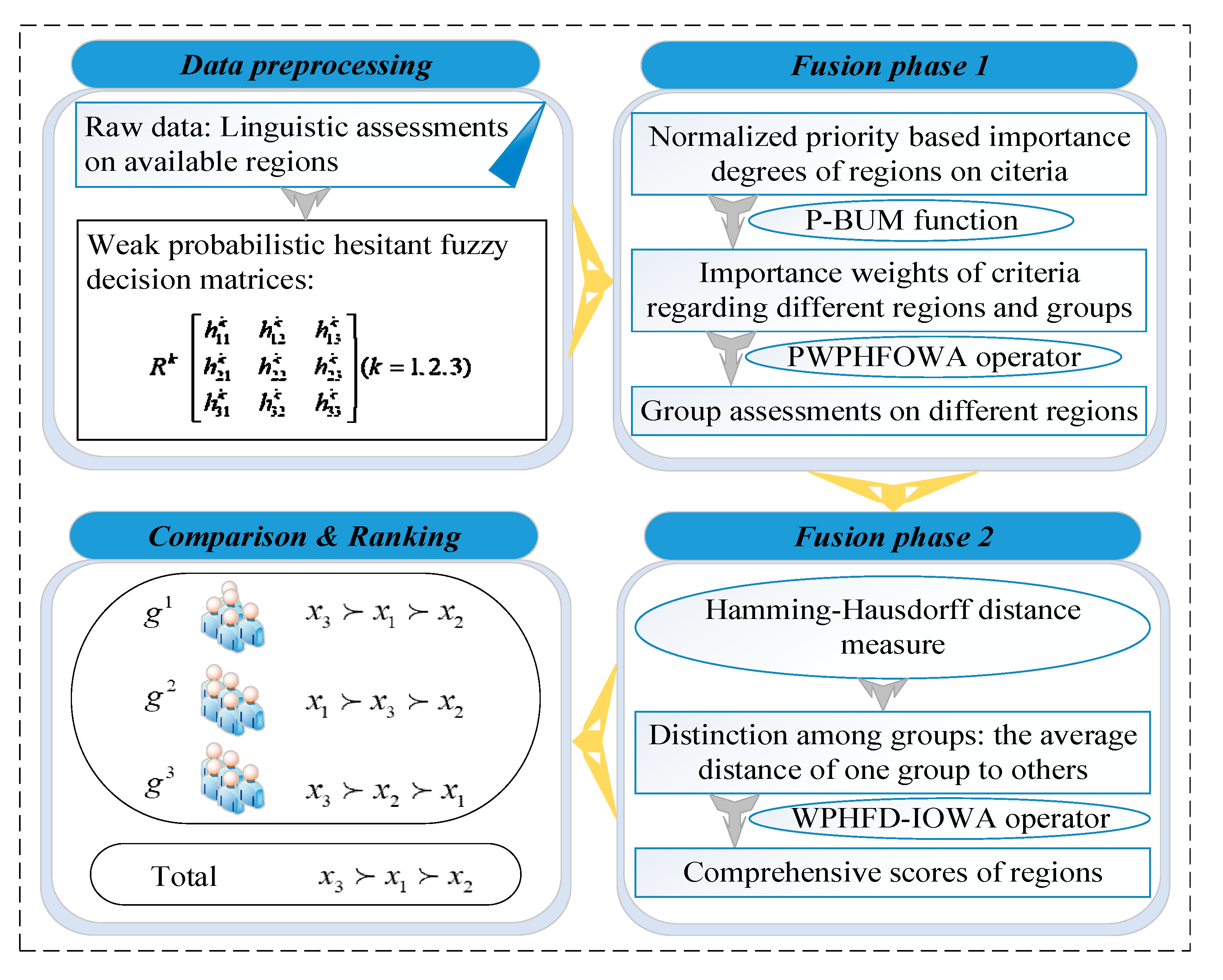
Clearly, the whole calculation process can be graphically described in Figure 2.

6. Discussion

This paper concentrates on handling MCGDM problems within weak P-HFEs and its application in the selection of an available sustainable DWSR. The outcome of this research may fulfill the research gaps mentioned in Section 2. Based on the previous illustration presented in Section 5, several findings and some comparisons with extant researches are observed and summarized as follows.

(1)

By comparison with other fuzzy sets in describing evaluation information [40,41] weak P-HFEs are more advantaged in expressing decision information in evaluating available DWSRs. This is because weak P-HFEs can simultaneously include positive negative opinions given by decision makers as well as the associated incomplete probabilistic information. Thus we apply weak P-HFEs to depict evaluation information about DWSRs ingeniously synthetic distinctive opinions in a decision group such that complaints about the ignorance of extreme opinion would not occur.

(2)

Indeed, it is always difficult to subjectively allocate satisfied weights to criteria and decision groups [25]. However, some existing studies that also focuses on weak P-HFEs have not considered this difficulty [18]. In our example of application, the importance weights of criteria and decision groups are objectively determined based on the original decision information. This avoids conflicts among decision makers when they stoutly believe that their opinions are not fairly treated.

(3)

Generally, there always exist priorities among criteria in realistic decision problems [31]. The developed evaluation approach fully considered this ubiquitous phenomenon that the aggregation process and the weight generation method are all introduced based on prioritized relationships provided by different decision groups.

(4)

The results objectively reflect some realistic and acquiescent decision rules and phenomena. Firstly, it is obvious that the ranking given by the management layer is entirely in accordance with that assessed by all decision makers. This indirectly identifies the critical position of the management layer. Secondly, as to the sales team, it can be observed in Table 5 that there is no consensus between the rankings generated by this group and the other two groups. In general, the sales team devotes to the sales quantity of the product that they may ignore the potential significance of policies that would aid the sustainable development of the company.

7. Conclusions

This paper conducts a research on investigating a hybrid evaluation approach with weak P-HFEs and performs a practical example of application. The strengths of the approach lie in the following points.

(1) The processing of the original decision data brings a broader understanding of how to address realistic evaluation problems with positive and negative information, which are asymmetrically distributed.

(2) Weights of criteria are decided based on the prioritization relationship of criteria given by different decision groups. In the meanwhile, we have considered the situation that the weights of the groups related to different alternatives should be distinctive, in case of cheating during the decision process. The objective determination of weights has brought a new way of identifying the importance degree without complaints.

(3) The fusion of decision information fully considers the phenomenon of asymmetric prioritization among different criteria, as well as the distinction between individuals that existed in reality.

(4) The proposed evaluation approach can serve as an emerging method for handling MCGDM problems with prioritized criteria and incomplete weight information within weak probabilistic hesitant fuzzy circumstance. It is totally possible to employ the proposed approach to solve other similar evaluation problems.

However, there still remains some work to be done. First, the alternative sustainable DWSRs in the example are all located in China, the applicability of the proposed method to managing other similar problems [42] remains to be further studied. Second, since the computational process of the weak P-HFEs is complicated, we need to further study the operations of weak P-HFEs. Except the above two points, the consensus between different groups should be taken into consideration. In future, we are going to conduct studies on these two aspects and devote our attention to applying the proposed approach to other fields, such as industrial engineering, E-commerce, and so on.

References

1. Chang, I.S.; Zhao, M.; Chen, Y.; Guo, X.; Zhu, Y.; Wu, J.; Yuan, T. Evaluation on the integrated water resources management in China’s major cities—Based on City Blueprint® Approach. J. Clean. Prod. 2020, 262, 121410. [Google Scholar] [CrossRef]
2. Chang, W.; Fu, C.; Feng, N.; Yang, S. Multi-criteria group decision making with various ordinal assessments. Group Decis. Negot. 2020. [Google Scholar] [CrossRef]
3. Peng, H.G.; Wang, J.Q.; Zhang, H.Y. Multi-criteria outranking method based on probability distribution with probabilistic linguistic information. Comput. Ind. Eng. 2020, 141, 106318. [Google Scholar] [CrossRef]
4. Zhang, X.; Wang, X.; Yu, S.; Wang, J.; Wang, T. Location selection of offshore wind power station by consensus decision framework using picture fuzzy modelling. J. Clean. Prod. 2018, 202, 980–992. [Google Scholar] [CrossRef]
5. Yager, R.R. Prioritized aggregation operators. Int. J. Approx. Reason. 2008, 48, 263–274. [Google Scholar] [CrossRef] [Green Version]
6. Ureña, R.; Chiclana, F.; Melançon, G.; Herrera-Viedma, E. A social network based approach for consensus achievement in multiperson decision making. Inf. Fusion 2019, 47, 72–87. [Google Scholar] [CrossRef] [Green Version]
7. Hou, F.; Triantaphyllou, E. An iterative approach for achieving consensus when ranking a finite set of alternatives by a group of experts. Eur. J. Oper. Res. 2019, 275, 570–579. [Google Scholar] [CrossRef]
8. Xu, Z.S.; Da, Q.L. An overview of operators for aggregating information. Int. J. Intell. Syst. 2003, 18, 953–969. [Google Scholar] [CrossRef]
9. Zadeh, L.A. Fuzzy sets. Inf. Control 1965, 8, 338–353. [Google Scholar] [CrossRef] [Green Version]
10. Yu, S.M.; Wang, J.; Wang, J.Q. An extended TODIM approach with intuitionistic linguistic numbers. Int. Trans. Oper. Res. 2018, 25, 781–805. [Google Scholar] [CrossRef]
11. Wang, J.; Wang, J.Q.; Tian, Z.P.; Zhao, D.Y. A multihesitant fuzzy linguistic multicriteria decision-making approach for logistics outsourcing with incomplete weight information. Int. Trans. Oper. Res. 2018, 25, 831–856. [Google Scholar] [CrossRef] [Green Version]
12. Tian, Z.P.; Wang, J.; Wang, J.Q.; Zhang, H.Y. Simplified neutrosophic linguistic multi-criteria group decision-making approach to green product development. Group Decis. Negot. 2017, 26, 597–627. [Google Scholar] [CrossRef]
13. Shaik, M.N.; Abdul-Kader, W. A hybrid multiple criteria decision making approach for measuring comprehensive performance of reverse logistics enterprises. Comput. Ind. Eng. 2018, 123, 9–25. [Google Scholar] [CrossRef]
14. Wang, J.Q.; Peng, J.J.; Zhang, H.Y.; Liu, T.; Chen, X.H. An uncertain linguistic multi-criteria group decision-making method based on a cloud model. Group Decis. Negot. 2015, 24, 171–192. [Google Scholar] [CrossRef]
15. Yu, S.M.; Wang, J.; Wang, J.Q.; Li, L. A multi-criteria decision-making model for hotel selection with linguistic distribution assessments. Appl. Soft Comput. 2018, 741–755. [Google Scholar] [CrossRef]
16. Zhang, X.; Wang, J.; Zhang, H.; Hu, J. A heterogeneous linguistic MAGDM framework to classroom teaching quality evaluation. EURASIA J. Math. Sci. Technol. Educ. 2017, 13, 4929–4956. [Google Scholar] [CrossRef]
17. Zhang, X.Y.; Wang, J.Q.; Hu, J.H. A consensus approach to multi-granular linguistic MCGDM with hesitant fuzzy linguistic information by using projection. J. Intell. Fuzzy Syst. 2018, 34, 1959–1974. [Google Scholar] [CrossRef]
18. Zhang, S.; Xu, Z.; He, Y. Operations and integrations of probabilistic hesitant fuzzy information in decision making. Inf. Fusion 2017, 38, 1–11. [Google Scholar] [CrossRef]
19. Torra, V. Hesitant fuzzy sets. Int. J. Intell. Syst. 2010, 25, 529–539. [Google Scholar] [CrossRef]
20. Zhu, B. Decision Method for Research and Application Based on Preference Relation; Southeast University: Nanjing, China, 2014. [Google Scholar]
21. Xu, Z.; Zhou, W. Consensus building with a group of decision makers under the hesitant probabilistic fuzzy environment. Fuzzy Optim. Decis. Mak. 2016, 16, 481–503. [Google Scholar] [CrossRef]
22. Li, J.; Wang, J.Q. An extended QUALIFLEX method under probability hesitant fuzzy environment for selecting green suppliers. Int. J. Fuzzy Syst. 2017, 19, 1866–1879. [Google Scholar] [CrossRef]
23. Zhou, W.; Xu, Z. Group consistency and group decision making under uncertain probabilistic hesitant fuzzy preference environment. Inf. Sci. 2017, 414, 276–288. [Google Scholar] [CrossRef]
24. Gonzalez Cruz, C.; Naderpour, M.; Ramezani, F. Water resource selection and optimisation for shale gas developments in Australia: A combinatorial approach. Comput. Ind. Eng. 2018, 124, 1–11. [Google Scholar] [CrossRef]
25. Xu, Z. An overview of methods for determining OWA weights. Int. J. Intell. Syst. 2005, 20, 843–865. [Google Scholar] [CrossRef]
26. Zhang, S.; Jianjun, Z.; Xiaodi, L.; Chen, Y. Regret theory-based group decision-making with multidimensional preference and incomplete weight information. Inf. Fusion 2016, 31, 1–13. [Google Scholar] [CrossRef]
27. Düğenci, M. A new distance measure for interval valued intuitionistic fuzzy sets and its application to group decision making problems with incomplete weights information. Appl. Soft Comput. 2016, 41, 120–134. [Google Scholar] [CrossRef]
28. Dong, J.Y.; Yuan, F.F.; Wan, S.P. Extended VIKOR method for multiple criteria decision-making with linguistic hesitant fuzzy information. Comput. Ind. Eng. 2017, 112, 305–319. [Google Scholar] [CrossRef]
29. Zhang, X.Y.; Zhang, H.Y.; Wang, J.Q. Discussing incomplete 2-tuple fuzzy linguistic preference relations inmulti-granular linguistic MCGDM with unknown weight information. Soft Comput. 2019, 23, 2015–2032. [Google Scholar] [CrossRef]
30. Yager, R.R. Prioritized OWA aggregation. Fuzzy Optim. Decis. Mak. 2009, 8, 245–262. [Google Scholar] [CrossRef]
31. Wei, G. Hesitant fuzzy prioritized operators and their application to multiple attribute decision making. Knowl. Based Syst. 2012, 31, 176–182. [Google Scholar] [CrossRef]
32. Yu, D. Multi-criteria decision making based on generalized prioritized aggregation operators under intuitionistic fuzzy environment. Int. J. Fuzzy Syst. 2013, 15, 47–54. [Google Scholar]
33. Chen, T.Y. A prioritized aggregation operator-based approach to multiple criteria decision making using interval-valued intuitionistic fuzzy sets: A comparative perspective. Inf. Sci. 2014, 281, 97–112. [Google Scholar] [CrossRef]
34. Ji, P.; Wang, J.Q.; Zhang, H.Y. Frank prioritized Bonferroni mean operator with single-valued neutrosophic sets and its application in selecting third-party logistics providers. Neural Comput. Appl. 2018, 30, 799–823. [Google Scholar] [CrossRef]
35. Yager, R.R. Induced ordered weighted averaging operators. IEEE Trans. Syst. Man Cybern. Part B Cybern. 1999, 29, 141–150. [Google Scholar] [CrossRef]
36. Xu, Z.; Chen, J. Ordered weighted distance measure. J. Syst. Sci. Syst. Eng. 2008, 17, 432–445. [Google Scholar] [CrossRef]
37. Farhadinia, B.; Xu, Z. Distance and aggregation-based methodologies for hesitant fuzzy decision making. Cogn. Comput. 2017, 9, 81–94. [Google Scholar] [CrossRef]
38. Radkani, E.; Hashemi, S.; Keshavarz-Haddad, A.; Haeri, M.A. An entropy-based distance measure for analyzing and detecting metamorphic malware. Appl. Intell. 2018, 48, 1536–1546. [Google Scholar] [CrossRef]
39. Yager, R.R. Quantifier guided aggregation using OWA operators. Int. J. Intell. Syst. 1996, 11, 49–73. [Google Scholar] [CrossRef]
40. Rostamzadeh, R.; Ghorabaee, M.K.; Govindan, K.; Esmaeili, A.; Nobar, H.B.K. Evaluation of sustainable supply chain risk management using an integrated fuzzy TOPSIS- CRITIC approach. J. Clean. Prod. 2018, 175, 651–669. [Google Scholar] [CrossRef]
41. Lin, M.; Huang, C.; Xu, Z. MULTIMOORA based MCDM model for site selection of car sharing station under picture fuzzy environment. Sustain. Cities Soc. 2020, 53, 101873. [Google Scholar] [CrossRef]
42. Kazak, J.K.; van Hoof, J. Decision support systems for a sustainable management of the indoor and built environment. Indoor Built Environ. 2018, 27, 1303–1306. [Google Scholar] [CrossRef] [Green Version]
Figure 1. Flow of the systematical evaluation approach.
Symmetry 12 01303 g001
Figure 2. Framework of the solving process.
Symmetry 12 01303 g002