Computing the Closest Approach Distance of Two Ellipsoids

Abstract

This paper presents two practical methods for computing the closest approach distance of two ellipsoids in their inter-center direction. The closest approach distance is crucial for collision handling in the dynamic simulation of rigid and deformable bodies approximated with ellipsoids. To find the closest approach distance, we formulate a set of equations for two ellipsoids contacting each other externally in terms of the inter-center distance, contact point, and normal vector. The equations are solved robustly and efficiently using a hybrid of the fixed-point iteration method and bisection method with root bracketing, and a hybrid of Newton’s method and the bisection method. In addition to a stopping criterion expressed with the progress of the solution, we introduce a novel criterion expressed in terms of the error in distance. This criterion can be effectively employed in real-time applications such as computer games by allowing an unnoticeable error. Experimental results demonstrate the robustness and efficiency of the proposed methods in various experiments.

1. Introduction

Recently, several techniques have been proposed to increase the speed of physics-based dynamic simulation by approximating rigid and deformable bodies with ellipsoids for interactive applications such as computer games [1,2,3]. Computing the closest approach distance between two ellipsoids in their inter-center direction is a key technique for collision handling among ellipsoids.

Given the positions and orientations of two ellipsoids, their overlap can be determined in a relatively easy manner by examining the signs of the solutions of their quartic characteristic equation without obtaining the actual solutions [4,5,6,7]. However, it is not easy to separate two overlapping ellipsoids. Position-based dynamics with ellipsoids [1] takes an approach that translates two ellipsoids outward along their inter-center direction by the closest approach distance to make them contact each other externally. To find the closest approach distance, a set of equations is formulated intuitively in terms of the inter-center distance, contact point, and contact normal vector. However, there is an error in the derivation of this solution; consequently, the solution is correct only for two spheres. In this paper, we rectify this error to find the closest approach distance correctly and intuitively. In [2,3], the method to compute the closest approach distance is not described.

The closest approach distance between two ellipsoids also plays important roles in the simulation of liquid crystals and colloidal systems [8,9,10,11,12]. In [10], an indirect formulation was introduced with the optimization of the elliptic contact function proposed in [8,9]. However, the derivation was complicated, and the numerical solution method was not addressed. In the method proposed in [12], the golden section search is employed with an analytic method [11] that computes the closest approach distance between two ellipses formed by the cross-section of two ellipsoids with a plane rotating about the line joining their centers. However, this method is considerably slow.

This paper presents two robust and efficient methods for computing the closest approach distance between two ellipsoids within a user-specified tolerance. The proposed methods are based on the intuitive approach introduced in position-based dynamics with ellipsoids [1]. We formulate the problem with a set of conditions in terms of the inter-center distance, contact point, and contact normal vector of two externally-contacting ellipsoids. The resulting equations are solved robustly and efficiently using a hybrid of the fixed-point iteration method and bisection method with root bracketing, and a hybrid of Newton’s method and the bisection method. In addition to a stopping criterion expressed with the change of the solution in a single solver iteration, we introduce a novel criterion expressed in terms of the actual error in distance. This can be effectively employed to increase the efficiency of the proposed methods in real-time applications such as computer games by allowing unnoticeable interferences between ellipsoids.

2. Method

2.1. Problem

Two ellipsoids can contact each other externally at a point by moving the center of one ellipsoid along their inter-center direction. The inter-center distance d in this circumstance is the closest approach distance of the two ellipsoids in their inter-center direction. The objective of the study was to develop a method that computes the distance d efficiently.

To formulate the closest approach distance, we first describe the shapes of two ellipsoids: $e_1$ and $e_2$. Each ellipsoid $e_i$ has three pairwise perpendicular unit axes of symmetry denoted by ${\mathbf{e}}_i^a,{\mathbf{e}}_i^b$, and ${\mathbf{e}}_i^c$, and the corresponding principal radii denoted by $a_i,b_i$, and $c_i$ in decreasing order. For convenience of derivation, we introduce the following quadratic functions for the ellipsoids:

$$e_1\left(\mathbf{x}\right)={\mathbf{x}}^{\mathrm{T}}{\mathbf{E}}_1\mathbf{x}\mathrm{and}{e}_2\left(\mathbf{x}\right)={\mathbf{x}}^{\mathrm{T}}{\mathbf{E}}_2\mathbf{x},$$

(1)

where ${\mathbf{E}}_i={\mathbf{R}}_i\mathrm{diag}(a_i^{-2},b_i^{-2},c_i^{-2}){\mathbf{R}}_i^{\mathrm{T}}$ is a symmetric matrix and ${\mathbf{R}}_i=[{\mathbf{e}}_i^a|{\mathbf{e}}_i^b\left|{\mathbf{e}}_i^c\right]$ is a $3\times 3$ rotation matrix. Thus, the shape of the ellipsoid $e_i$ centered at the origin can be described by the point $\mathbf{x}$ that satisfies $\mathbf{x}{\mathbf{E}}_i{\mathbf{x}}^{\mathrm{T}}=1$.

The closest approach distance of two ellipsoids in their inter-center direction is invariant under translation. Given two ellipsoids, we displace both ellipsoids at the same time such that one ellipsoid is centered at the origin and the other ellipsoid maintains its relative direction and distance. We assume that $e_1$ is centered at the origin and $\mathbf{n}$ is the unit direction vector from the center of $e_1$ to the center of $e_2$. When the two ellipsoids touch each other externally at a contact point $\mathbf{x}$ by approaching in the direction $\mathbf{n}$ with the inter-center distance d, the center of $e_2$ is apart from the center of $e_1$ by $d\mathbf{n}$. At this moment, $\mathbf{x}$ should be a point on $e_1$ and $e_2$. Thus, $\mathbf{x}$ and d should satisfy the following two conditions represented using the quadratic functions given in Equation (1):

$$\begin{array}{cc}\hfill e_1\left(\mathbf{x}\right)& =1,\hfill \end{array}$$

(2)

$$\begin{array}{cc}\hfill e_2(\mathbf{x}-d\mathbf{n})& =1.\hfill \end{array}$$

(3)

In addition, for the two ellipsoids to contact each other externally at $\mathbf{x}$, the tangent planes of $e_1$ and $e_2$ at $\mathbf{x}$ should be parallel with opposite normal directions. That is, the gradient vectors of $e_1$ and $e_2$ at $\mathbf{x}$ should be parallel with opposite directions. Thus, the following condition for the gradient vectors should also be satisfied:

$$\nabla e_1\left(\mathbf{x}\right)=\left(\frac{u}{u-1}\right)\nabla e_2(\mathbf{x}-d\mathbf{n}),\mathrm{for}u\in [0,1),$$

(4)

where ∇ denotes the spatial derivative with respect to $\mathbf{x}$, and $u/(u-1)\in (-\infty ,0]$ makes the gradient vectors have opposite directions. Here, $u/(u-1)$ was adopted, unlike $\lambda \in (-\infty ,0]$ in [1], to make the range of u finite, such that a bracketing method can be employed for root finding. Finally, the computation of the closest approach distance d requires the determination of u and $\mathbf{x}$ that satisfies all three conditions given in Equations (2)–(4).

2.2. Solution Method

The substitution of the gradient vectors of the quadratic functions given in Equation (1) into Equation (4) yields

$${\mathbf{E}}_1\mathbf{x}=\left(\frac{u}{u-1}\right){\mathbf{E}}_2(\mathbf{x}-d\mathbf{n}).$$

(5)

Manipulating Equation (5) for $\mathbf{x}$, we can obtain

$$\mathbf{x}=ud\mathbf{w}\left(u\right),$$

(6)

where $\mathbf{w}\left(u\right)$ is introduced for compact representation of $\mathbf{x}$:

$$\mathbf{w}\left(u\right)={\left[(1-u){\mathbf{E}}_1+u{\mathbf{E}}_2\right]}^{-1}{\mathbf{E}}_2\mathbf{n}.$$

(7)

In Equation (6), $\mathbf{x}$ is dependent on u and d. However, we consider $\mathbf{x}$ as a function of only u for the moment with the assumption that d is known. As illustrated in Figure 1, $\mathbf{x}\left(u\right)$ moves along a curve that starts from the origin (the center of $e_1$) to $d\mathbf{n}$ (the center of $e_2$) as u varies from 0 to 1. Along this curve, the gradient vector $\nabla e_1\left(\mathbf{x}\right)$ is parallel to $\nabla e_2(\mathbf{x}-d\mathbf{n})$ in the opposite direction.

The contact point should be on both ellipsoids. The substitution of Equation (6) into Equations (2) and (3) yields

$$\begin{array}{cc}\hfill u^2\mathbf{w}{\left(u\right)}^{\mathrm{T}}{\mathbf{E}}_1\mathbf{w}\left(u\right)& =1/d^2,\hfill \end{array}$$

(8)

$$\begin{array}{cc}\hfill {(1-u)}^2\mathbf{w}{\left(u\right)}^{\mathrm{T}}\left[{\mathbf{E}}_1{\mathbf{E}}_2^{-1}{\mathbf{E}}_1\right]\mathbf{w}\left(u\right)& =1/d^2.\hfill \end{array}$$

(9)

Here, to derive Equation (9) in a compact form, Equation (5) was rearranged as $(\mathbf{x}-d\mathbf{n})=(u-1)/u{\mathbf{E}}_2^{-1}{\mathbf{E}}_1\mathbf{x}$ and then applied to Equation (3) with the property ${\mathbf{E}}_i^{\mathrm{T}}={\mathbf{E}}_i$. By subtracting each side of Equation (9) from Equation (8), we can eliminate d, and thus we no longer need the assumption that d is known. This results in the following sextic equation of $u\in (0,1]$:

$$f\left(u\right)=u^2\mathbf{w}{\left(u\right)}^{\mathrm{T}}{\mathbf{E}}_1\mathbf{w}\left(u\right)-{(1-u)}^2\mathbf{w}{\left(u\right)}^{\mathrm{T}}\left[{\mathbf{E}}_1{\mathbf{E}}_2^{-1}{\mathbf{E}}_1\right]\mathbf{w}\left(u\right)=0.$$

(10)

Once u is computed, $\mathbf{w}$ can be obtained from Equation (7), d from Equations (8) and (9), and finally $\mathbf{x}$ from Equation (6).

To solve Equation (10) for u, we propose two methods based on fixed-point iteration and Newton’s method. The former is easy to implement, but converges slowly for an accurate solution. The latter requires the derivative $f^{\prime }\left(u\right)$ as well as the function value $f\left(u\right)$, but converges quickly in general. However, when applied to real-time applications with an actual error tolerance that allows a relatively large but unnoticeable error as suggested in Section 2.3, the former converges as quickly as the latter.

A fixed-point iteration method can be obtained by manipulating Equation (10) with respect to u and exploiting $\mathbf{w}\left(u\right)$ at the previous iteration:

$$u_{i+1}=g\left(u_i\right)={\left[1+{\left(\frac{\mathbf{w}{\left(u_i\right)}^{\mathrm{T}}{\mathbf{E}}_1\mathbf{w}\left(u_i\right)}{\mathbf{w}{\left(u_i\right)}^{\mathrm{T}}\left[{\mathbf{E}}_1{\mathbf{E}}_2^{-1}{\mathbf{E}}_1\right]\mathbf{w}\left(u_i\right)}\right)}^{\frac{1}{2}}\right]}^{-1}.$$

(11)

In addition, the root bracketing property of the bisection method can be adopted because $u\in [0,1)$. Consequently, we can employ a hybrid of the fixed-point iteration and the bisection method as in Newton’s method [13] to guarantee the convergence. In contrast to our derivation, a similarity transform was incorrectly applied in [1] to an equation, corresponding to Equation (10) but formulated with $\lambda =u/(u-1)$, so that it became quadratic and could be solved analytically. However, this condition is true only for the case of two spheres. In [2,3], this mistake was rectified, and fixed-point iteration was employed to address the case of two ellipsoids. However, it was not described because collision detection between two ellipsoids was not the major concern. Furthermore, the formulation with $\lambda$ does not allow root bracketing; therefore, a hybrid approach with the bisection method cannot be employed.

To obtain an accurate solution of Equation (10), Brent’s method [13] can be employed with the function value $f\left(u\right)$ only, as suggested in [9]. However, for better convergence, we employ a hybrid of Newton’s method and the bisection method with root bracketing [13], which exploits the derivative $f^{\prime }\left(u\right)$ as well as the function value $f\left(u\right)$. To this end, we need an analytic form of $f^{\prime }\left(u\right)$. By employing the differentiation rule $\partial \left({\mathbf{A}}^{-1}\right)=-{\mathbf{A}}^{-1}(\partial \mathbf{A}){\mathbf{A}}^{-1}$ [14], we obtain

$$\begin{array}{c}\hfill f^{\prime }\left(u\right)=2u{\mathbf{w}}^{\mathrm{T}}\left[\mathbf{I}-u{\mathbf{E}}_{21}{\mathbf{E}}_u^{-1}\right]{\mathbf{E}}_1\mathbf{w}+2(1-u){\mathbf{w}}^{\mathrm{T}}\left[\mathbf{I}+(1-u){\mathbf{E}}_{21}{\mathbf{E}}_u^{-1}\right]{\mathbf{E}}_1{\mathbf{E}}_2^{-1}{\mathbf{E}}_1\mathbf{w},\end{array}$$

(12)

where ${\mathbf{E}}_{21}=({\mathbf{E}}_2-{\mathbf{E}}_1)$ and ${\mathbf{E}}_u=\left[(1-u){\mathbf{E}}_1+u{\mathbf{E}}_2\right]$.

2.3. Initial Guess and Stopping Criteria

A good initial guess is considerably important in reducing the number of solver iterations. From Figure 1, $u=0.5$ is a good initial guess because it is the exact solution when two ellipsoids are actually spheres with the same radius. For two spheres with different radii $a_1$ and $a_2$, $u=a_1/(a_1+a_2)$ is the exact solution, and thus it becomes a good initial guess for more general cases. This initial guess was employed in all the experiments.

For a stopping criterion, we can simply adopt the following popular one:

$$|u_i-u_{i-1}|<{ϵ}_u.$$

(13)

This determines whether the change of u in the i-th iteration is less than a user-specified tolerance ${ϵ}_u$. To reduce the number of iterations further, we introduce an additional actual error tolerance as a stopping criterion. The closest approach distance d can be obtained from u using Equations (8) and (9). Here, d should be positive when the two ellipsoids touch each other externally in the direction $\mathbf{n}$. Let $d_1$ and $d_2$ be the distances computed using Equations (8) and (9), respectively. Note that $d_1$ and $d_2$ can be different because of the numerical error in u. The contact points ${\mathbf{x}}_1$ and ${\mathbf{x}}_2$ on the two ellipsoids can be obtained by substituting u, $d_1$, and $d_2$ into Equation (6). Thus, we can employ a stopping criterion that determines whether the distance between the two contact points is within a user-specified tolerance at the i-th iteration:

$$\parallel {\mathbf{x}}_1^{\left(i\right)}-{\mathbf{x}}_2^{\left(i\right)}\parallel <{ϵ}_{\mathbf{x}}{r}_{min},$$

(14)

where $r_{min}$ is the minimum radius of the two ellipsoids. In real-time applications such as computer games, users generally do not notice interferences between ellipsoids with ${ϵ}_{\mathbf{x}}$ less than $1\%$. Consequently, the criterion given in Equation (14) is effective in reducing the number of iterations while allowing an unnoticeable numerical error with slight additional computation.

3. Experimental Results

We propose two methods to compute the closest approach distance of two ellipsoids. One method employs a hybrid of the bisection method with Newton’s method, and the other with fixed-point iteration. We call the former hybrid Newton’s method and the latter the hybrid fixed-point iteration method. In this section, we describe a performance comparison of four methods: (1) hybrid Newton’s method, (2) hybrid fixed-point iteration method, (3) Brent’s method with the elliptic contact potential [9], and (4) cross-section search [12] in various examples. The proposed methods were implemented using C++ and the Eigen library (eigen.tuxfamily.org) to perform the vector and matrix operations. All of the experiments were performed using a workstation equipped with a 2.3 GHz 18-core Intel Xeon W processor and 128 GB 2666 MHz DDR4 RAM.

The first experiment was conducted to test the number of solver iterations and the computation times for 10 million pairs of randomly generated ellipsoids. The ratio between the maximum and minimum radii of each ellipsoid was restricted to less than $\gamma$, and the ratio between the maximum radii in a pair of ellipsoids was restricted to less than $\Gamma$. The orientation of an ellipsoid and the inter-center direction between a pair of ellipsoids were generated randomly without any restriction. For robustness of physics-based simulation, $\gamma =2$ was used in [1] and $\gamma =5$ in [2,3]. Figure 2 shows the distributions of the numbers of solver iterations required for ${ϵ}_u={10}^{-8}$ for the four methods with $\gamma =3$ and $\Gamma =3$. The average and maximum number of solver iterations and the average computation time are listed in

Table 1. Maximum and average number of solver iterations and average computation time in ns. $t_1$ and $t_{18}$ are times in nanoseconds using a single core with a single thread and 18 cores with 36 threads, respectively.

	Figure 2				Figure 6
	$|{\mathbf{u}}_{\mathbf{i}}-{\mathbf{u}}_{\mathbf{i}-\mathbf{1}}|<{\mathbf{10}}^{-\mathbf{8}}$				$|{\mathbf{u}}_{\mathbf{i}}-{\mathbf{u}}_{\mathbf{i}-\mathbf{1}}|<{\mathbf{10}}^{-\mathbf{8}}$						$\parallel {\mathbf{x}}_{\mathbf{1}}^{\left(\mathbf{i}\right)}-{\mathbf{x}}_{\mathbf{2}}^{\left(\mathbf{i}\right)}\parallel <{\mathbf{10}}^{-\mathbf{2}}{\mathit{r}}_{\mathit{m}\mathit{i}\mathit{n}}$
	# Solver Iters.		Time		# Solver Iters.			Time			# Solver Iters.			Time
	Max.	Avg.	${\mathit{t}}_{\mathbf{1}}$		Max.	Avg.		${\mathit{t}}_{\mathbf{1}}$	${\mathit{t}}_{\mathbf{18}}$		Max.	Avg.		${\mathit{t}}_{\mathbf{1}}$	${\mathit{t}}_{\mathbf{18}}$
Hybrid Newton’s Method	14	4.30	310		14	3.87		285	12.7		13	2.46		205	9.4
Hybrid Fixed-Point Iteration Method	28	7.37	491		28	6.07		433	16.9		10	2.43		189	8.7
Brent’s Method	28	11.62	578		29	11.21		553	22.0		12	4.99		487	20.8
Cross-Section Search	41	40.34	16,914		-	-		-	-		-	-		-	-

. The computation time was measured using a single core in this experiment. The hybrid Newton’s method performed better than the others in all aspects.

The error in the analytic method for the closest approach distance of two ellipses increased as $\gamma$ increased [11]. Correspondingly, the error in the cross-section search [12] also increased, regardless of the number of solver iterations in the golden section search that found the angle of the cross section resulting in the closest approach distance of two ellipsoids. In contrast, the other methods computed the closest approach distance within a user-specified tolerance even with a large $\gamma$. However, the number of solver iterations increased as $\gamma$ increased. This result was verified with the second experiment, in which the closest approach distances were computed for each of the 1 million pairs of ellipsoids generated randomly with $\gamma$ increasing from 1 to 200 and $\Gamma$ fixed at 3. For the stopping criterion, we employed Equation (13) with ${ϵ}_u={10}^{-8}$ and the maximum number of solver iterations set to 100. Figure 3 shows the maximum and average number of solver iterations. In the traditional fixed-point iteration method, the number of solver iterations exceeded 100 when $\gamma$ became larger than 7. However, the hybrid fixed-point iteration method was robust, even when $\gamma$ reached 200, with an average of 11.3 solver iterations. The hybrid Newton’s and Brent’s methods were also robust and reached $\gamma =200$ with an average of 5.6 and 13.0 solver iterations, respectively. $\gamma =200$ implied the maximum radius could be 200 times larger than the minimum in a single ellipsoid, and thus it was sufficient for physics-based simulation with ellipsoids.

The number of solver iterations was almost insensitive to $\Gamma$ in contrast to $\gamma$. Figure 4 shows the maximum and average number of solver iterations required to compute the closest approach distances for each of the 1 million pairs of ellipsoids generated randomly, with $\Gamma$ increasing from 1 to 200 and $\gamma$ fixed at 3. We can observe that the computation time was almost insensitive to $\Gamma$, the proportion between the gross sizes of the ellipsoids. Consequently, the proposed methods could be effectively used for simulating ellipsoids with various sizes.

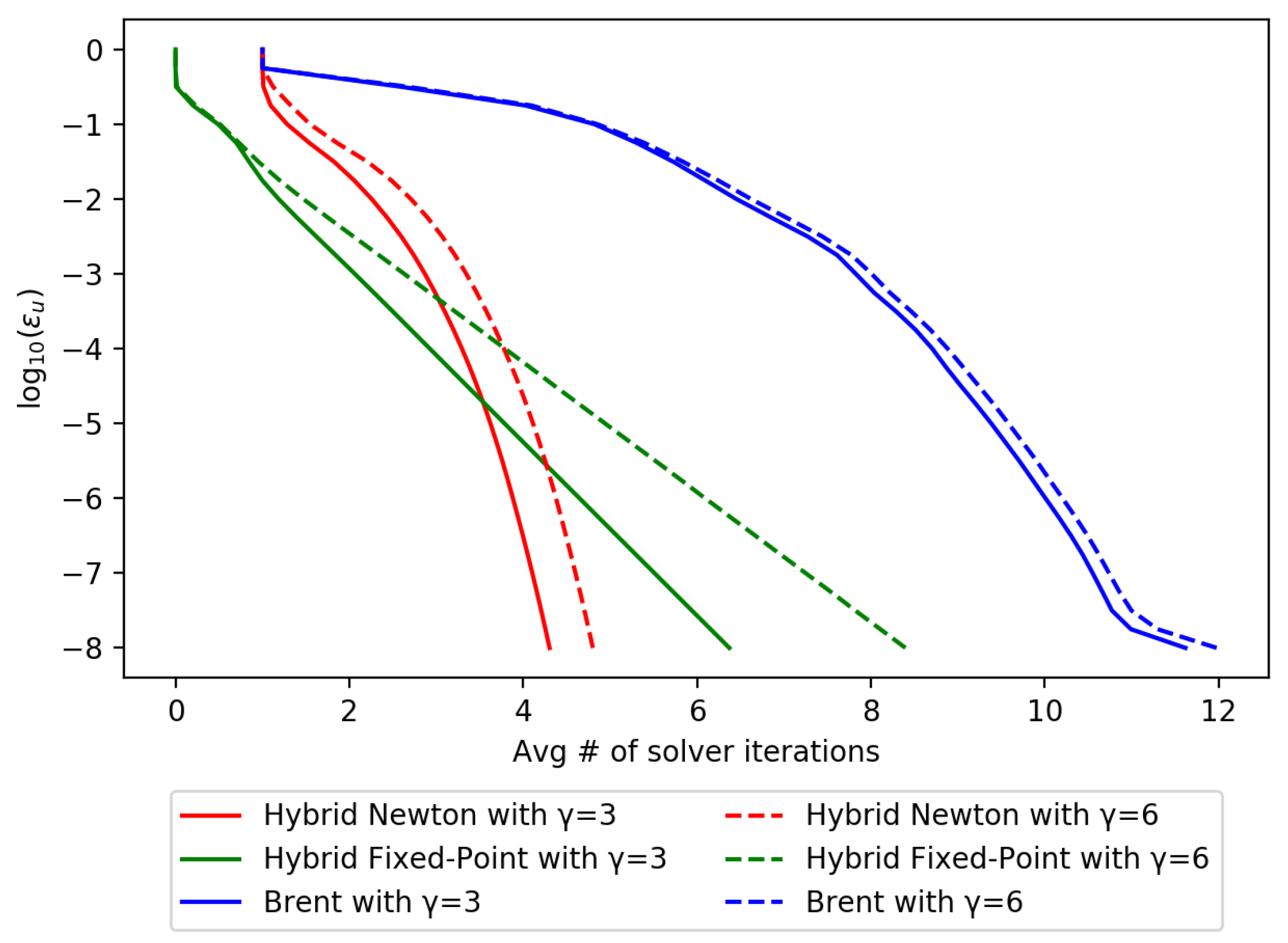
The next experiment was conducted to test the number of solver iterations with respect to the error tolerance. Figure 5 shows the average number of solver iterations required to compute the closest approach distances for 1 million pairs of random ellipsoids with $\gamma =3$ (solid lines) and $\gamma =6$ (dashed lines) when ${ϵ}_u$ decreases from 1 to ${10}^{-8}$. $\Gamma$ was fixed at 3. The hybrid Newton’s and Brent’s methods exhibited quadratic convergence, whereas the hybrid fixed-point iteration method exhibited linear convergence. However, when $\gamma$ was small and the error tolerance was large, the hybrid fixed-point iteration method performed better than the others. This observation can be effectively exploited with the actual error tolerance given in Equation (14) as illustrated in the final experiment.

The final experiment demonstrated the effectiveness of the proposed methods in real-time as-rigid-as-possible dynamic simulation of deformable bodies approximated with ellipsoids [3]. Figure 6 shows the simulation result of 180 deformable bodies approximated with 4404 ellipsoids. A spatial subdivision technique [15] was employed to reduce the number of collision tests between a pair of ellipsoids, and 49,716,944 collision tests were performed during 60 s of simulation. The ratios $\gamma$ and $\Gamma$ between radii were 4.86 and 2.55, respectively. Table 1 lists the average and maximum number of solver iterations and the average computation time required to satisfy the stopping criterion given in Equation (13) with ${ϵ}_u={10}^{-8}$. The computation time was measured in two different manners that exploited (1) a single core and (2) all 18 cores with a simple parallelization using OpenMP. In both cases, the hybrid Newton’s method was the most efficient.

In real-time applications such as computer games, computational efficiency has higher priority over simulation accuracy. Moreover, the interference between ellipsoids was scarcely noticeable even when the interference was $1\%$ of the minimum radius. Thus, the actual error tolerance given in Equation (14) was adequate as a stopping criterion. Table 1 lists the average and maximum number of solver iterations and the average computation time when ${ϵ}_{\mathbf{x}}={10}^{-2}$. With the actual error tolerance, the hybrid fixed-point iteration method was shown to be the most efficient. From this experiment, we can conclude that the hybrid Newton’s method is a good choice when the accuracy is important, and the hybrid fixed-point iteration method is a good choice in real-time applications.

4. Conclusions

The computation of the closest approach distance of two ellipsoids in their inter-center direction is crucial for collision handling among ellipsoids that approximate rigid and deformable bodies in physics-based dynamics simulation [1,2,3] and also plays important roles in the simulation of liquid crystals and colloidal systems [8,9,10,11,12]. We proposed two intuitive and efficient methods to compute the closest approach distance of two ellipsoids. Based on the intuitive approach introduced in position-based dynamics with ellipsoids [1], we formulated a set of equations for two ellipsoids contacting each other externally with the inter-center distance, contact point, and normal vector. The equations can be solved accurately and efficiently using a hybrid of Newton’s method and bisection method with root bracketing. In addition, we introduced a novel criterion expressed in terms of the error in distance. Our experimental results demonstrate that this criterion can be effectively employed in real-time applications such as computer games by allowing an unnoticeable error with a hybrid of the fixed-point iteration method and bisection method. Currently, our methods deal with only static ellipsoids. We plan to extend our methods to cope with moving ellipsoids.

References

- Müller, M.; Chentanez, N. Solid Simulation with Oriented Particles. ACM Trans. Graph. 2011, 30, 92. [Google Scholar] [CrossRef]
- Choi, M.G. Real-Time Simulation of Ductile Fracture with Oriented Particles. Comput. Anim. Virtual Worlds 2014, 25, 455–463. [Google Scholar] [CrossRef]
- Choi, M.G.; Lee, J. As-Rigid-As-Possible Solid Simulation with Oriented Particles. Comput. Graph. 2018, 70, 1–7. [Google Scholar] [CrossRef]
- Wang, W.; Wang, J.; Kim, M.S. An Algebraic Condition for the Separation of Two Ellipsoids. Comput. Aided Geom. Des. 2001, 18, 531–539. [Google Scholar] [CrossRef]
- Choi, Y.K.; Chang, J.W.; Wang, W.; Kim, M.S.; Elber, G. Continuous collision detection for ellipsoids. IEEE Trans. Vis. Comput. Graph. 2009, 15, 311–324. [Google Scholar] [CrossRef] [PubMed] [Green Version]
- Jia, X.; Choi, Y.K.; Mourrain, B.; Wang, W. An algebraic approach to continuous collision detection for ellipsoids. Comput. Aided Geom. Des. 2011, 28, 164–176. [Google Scholar] [CrossRef] [Green Version]
- Gonzalez-Vega, L.; Mainar, E. Solving the separation problem for two ellipsoids involving only the evaluation of six polynomials. In Proceedings of the Milestones in Computer Algebra, London, ON, Canada, 1–3 May 2008; pp. 201–208. [Google Scholar]
- Perram, J.W.; Wertheim, M.S. Statistical Mechanics of Hard Ellipsoids. I. Overlap Algorithm and the Contact Function. J. Comput. Phys. 1985, 58, 409–416. [Google Scholar] [CrossRef]
- Perram, J.W.; Rasmussen, J.; Præstgaard, E.; Lebowitz, J.L. Ellipsoid contact potential: Theory and relation to overlap potentials. Phys. Rev. E 1996, 54, 6565–6572. [Google Scholar] [CrossRef] [PubMed] [Green Version]
- Paramonov, L.; Yaliraki, S.N. The directional contact distance of two ellipsoids: Coarse-grained potentials for anisotropic interactions. J. Chem. Phys. 2005, 123, 194111. [Google Scholar] [CrossRef] [PubMed] [Green Version]
- Zheng, X.; Palffy-Muhoray, P. Distance of closest approach of two arbitrary hard ellipses in two dimensions. Phys. Rev. E 2007, 75, 061709. [Google Scholar] [CrossRef] [PubMed] [Green Version]
- Zheng, X.; Iglesias, W.; Palffy-Muhoray, P. Distance of Closest Approach of Two Arbitrary Hard Ellipsoids. Phys. Rev. E 2009, 79, 057702. [Google Scholar] [CrossRef] [PubMed] [Green Version]
- Press, W.H.; Teukolsky, S.A.; Vetterling, W.T.; Flannery, B.P. Numerical Recipes: The Art of Scientific Computing, 3rd ed.; Cambridge University: Cambridge, UK, 2007. [Google Scholar]
- Petersen, K.B.; Pedersen, M.S. The Matrix Cookbook; Technical University of Denmark: Kongens Lyngby, Denmark, 2012. [Google Scholar]
- Teschner, M.; Heidelberger, B.; Müller, M.; Pomeranets, D.; Gross, M. Optimized spatial hashing for collision detection of deformable objects. In Proceedings of the 8th Workshop on Vision, Modeling, and Visualization, Munich, Germany, 19–21 November 2003; pp. 47–54. [Google Scholar]
Figure 1.
Two contacting ellipsoids and with the closest approach distance d in the inter-center direction and their concentric ellipsoids (with the same aspect ratios) contacting along the curve where the gradient vectors and are parallel.
Figure 2.
Distributions of the number of solver iterations with for 10 million pairs of ellipsoids generated randomly with and .
Figure 3.
Maximum and average number of solver iterations for 1 million samples generated for each value from 1 to 200.
Figure 4.
Figure 5.
Average number of solver iterations for 1 million samples when decreases from 1 to . The solid lines are for , and the dashed lines are for .
Figure 6.
Real-time simulation of 180 deformable models (top) with 4404 ellipsoidal particles (bottom) using the as-rigid-as-possible solid simulation technique presented in [3].