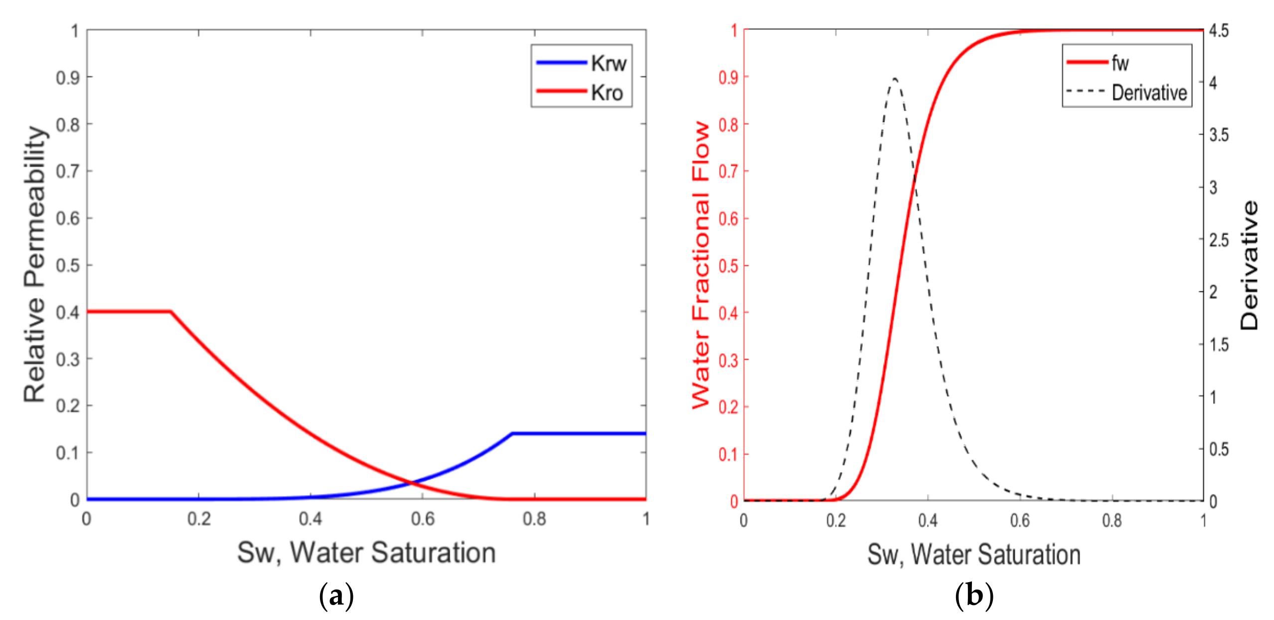
Figure 1.
(
a) Water–oil two-phase relative permeability; and (
b) Fractional flow of water and its derivative as a function of water saturation based on parameters in
Table 2.
Figure 1.
(
a) Water–oil two-phase relative permeability; and (
b) Fractional flow of water and its derivative as a function of water saturation based on parameters in
Table 2.
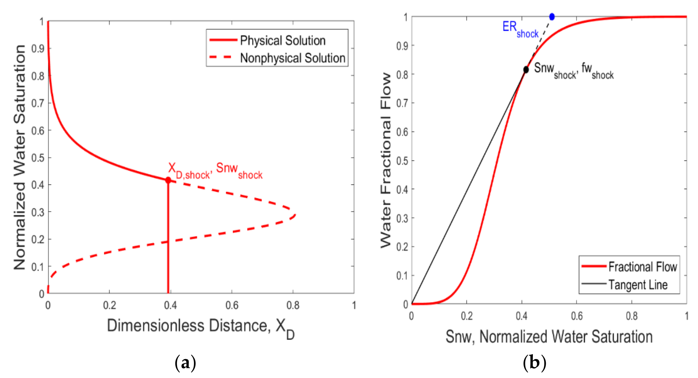
Figure 2.
Determination of the shock front by (
a) Material balance and (
b) Welge graphical method, parameters are listed in
Table 2.
Figure 2.
Determination of the shock front by (
a) Material balance and (
b) Welge graphical method, parameters are listed in
Table 2.
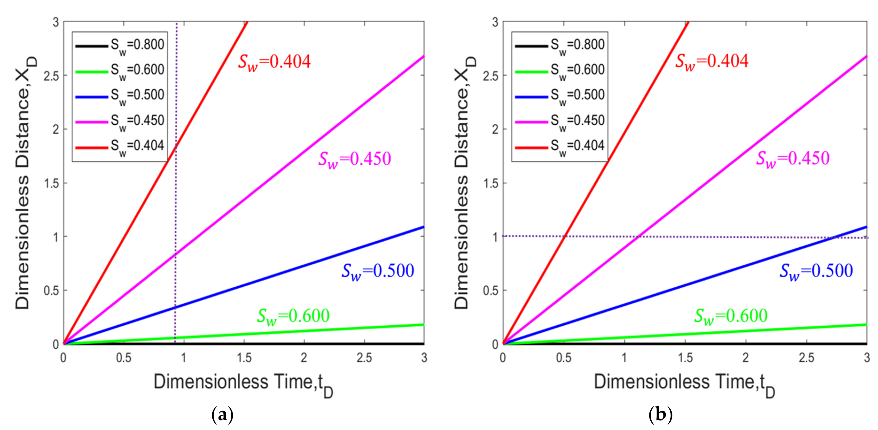
Figure 3.
Trajectory of constant water saturation in distance time diagram; (a) Construction of saturation profile plot, and (b) Construction of effluent history plot.
Figure 3.
Trajectory of constant water saturation in distance time diagram; (a) Construction of saturation profile plot, and (b) Construction of effluent history plot.
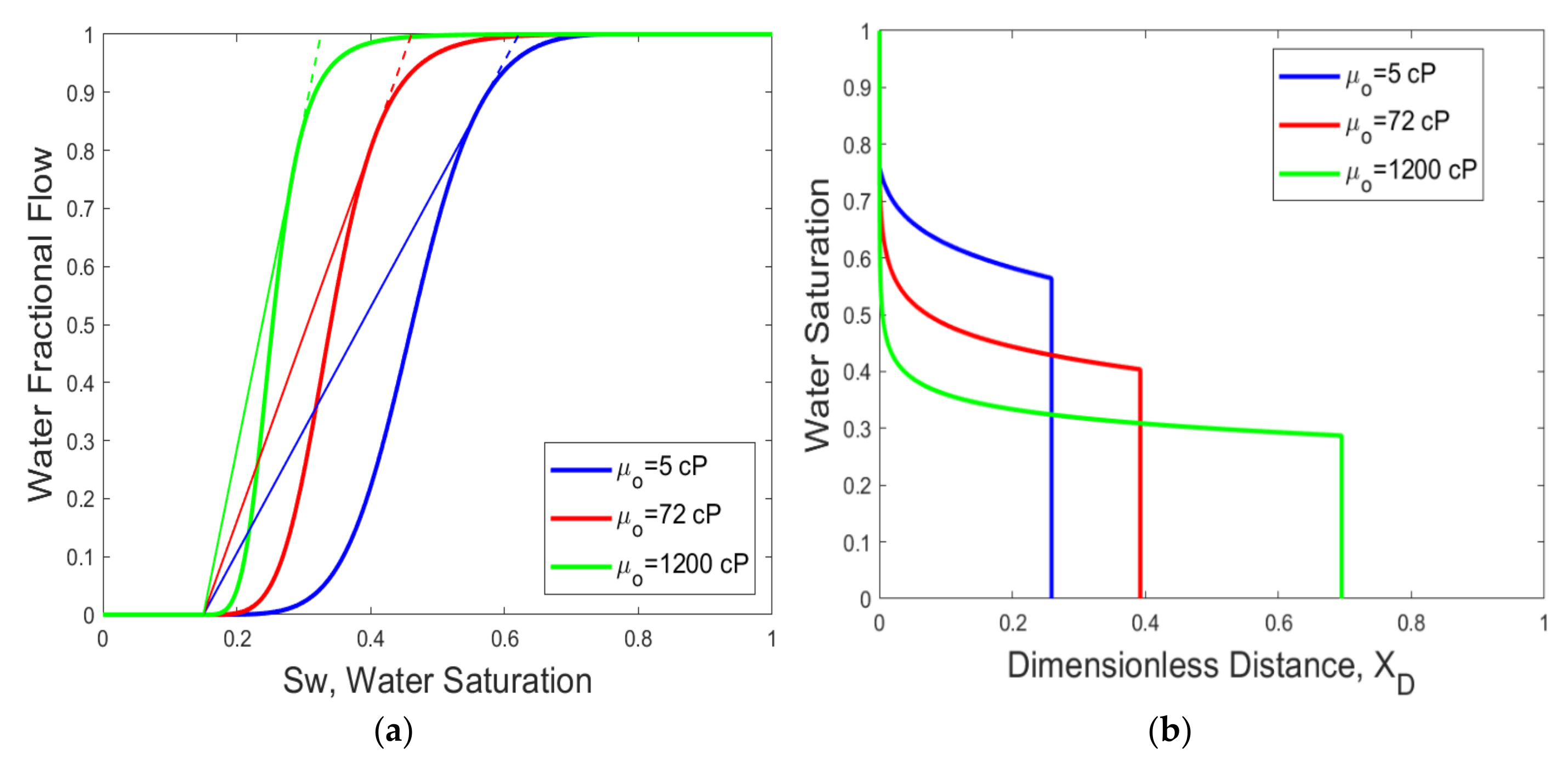
Figure 4.
(a) Water fractional flow as a function of oil viscosity and construction of shock front; and (b) Water saturation profile at tD = 0.20 PV as a function of different oil viscosity during water flooding. The lines in green, red, and blue represent the cases of water flooding with high oil viscosity, moderate oil viscosity, and low oil viscosity, respectively.
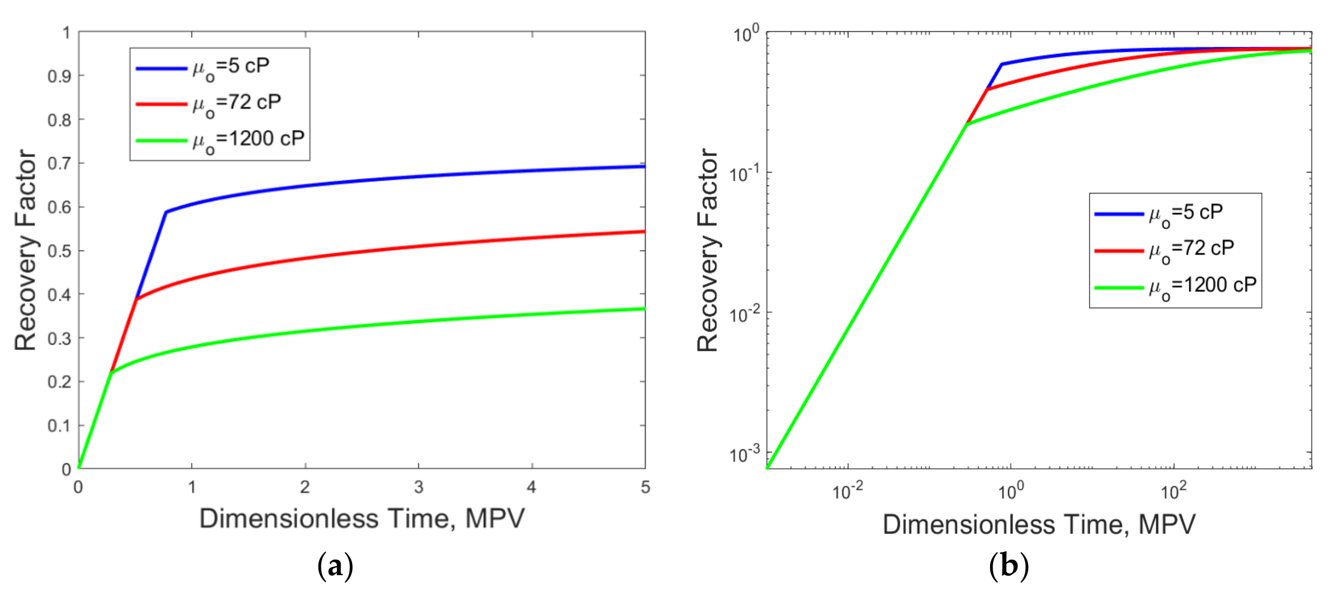
Figure 5.
Oil recovery history at (a) normal scale and (b) logarithm scale as a function of oil viscosity during water flooding. The lines in green, red, and blue represent the cases of water flooding with high oil viscosity, moderate oil viscosity, and low oil viscosity, respectively.
Figure 5.
Oil recovery history at (a) normal scale and (b) logarithm scale as a function of oil viscosity during water flooding. The lines in green, red, and blue represent the cases of water flooding with high oil viscosity, moderate oil viscosity, and low oil viscosity, respectively.
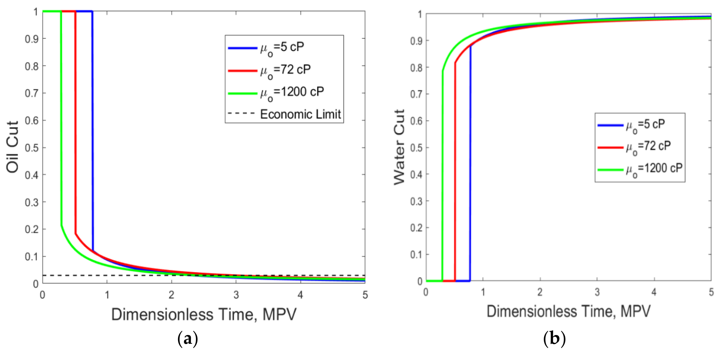
Figure 6.
(a) Water cut history and (b) oil cut history during water injection up to 5.0 PV for different oil viscosity. The lines in green, red, and blue represent the cases of water flooding with high oil viscosity, moderate oil viscosity, and low oil viscosity, respectively.
Figure 6.
(a) Water cut history and (b) oil cut history during water injection up to 5.0 PV for different oil viscosity. The lines in green, red, and blue represent the cases of water flooding with high oil viscosity, moderate oil viscosity, and low oil viscosity, respectively.
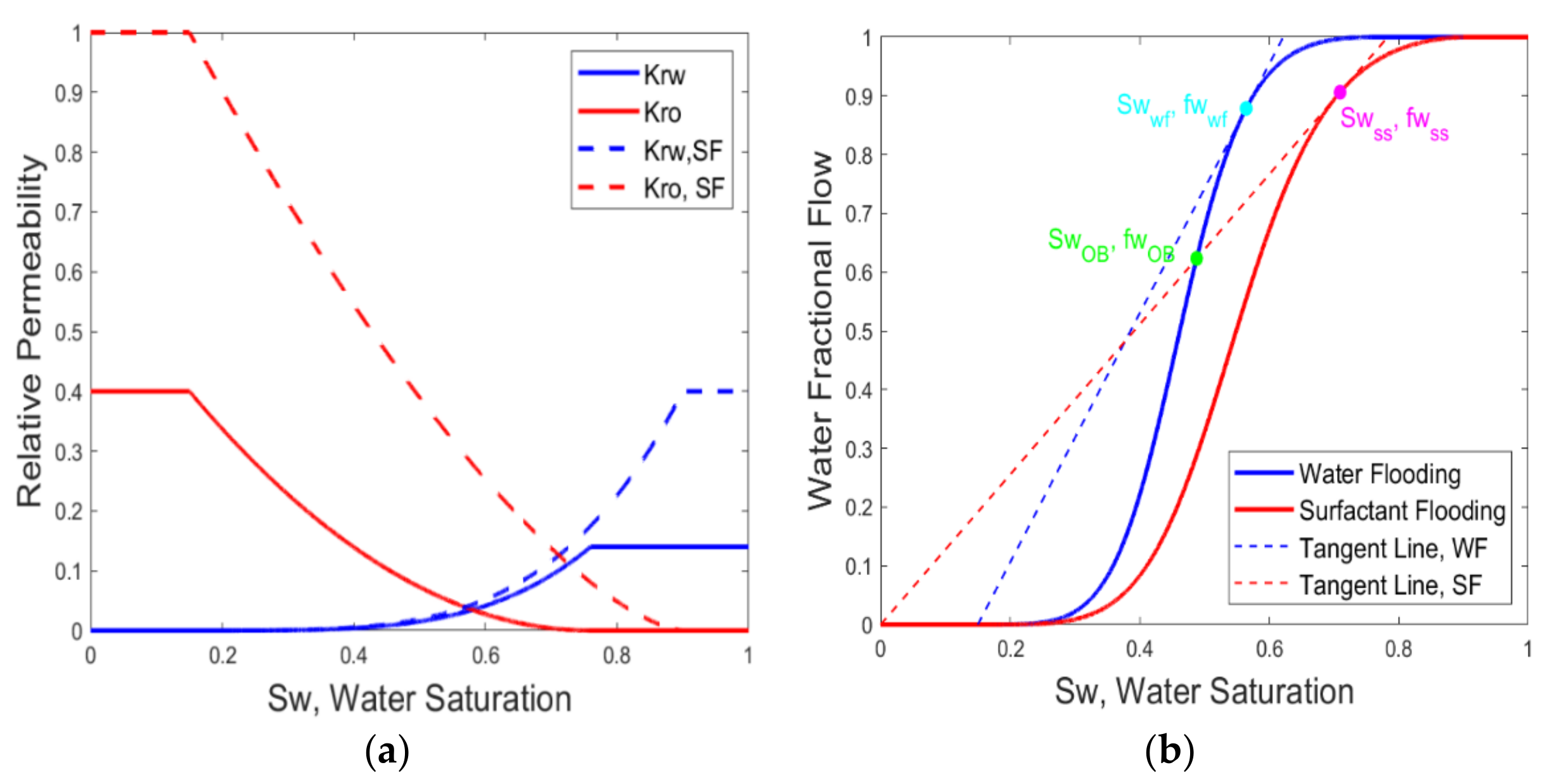
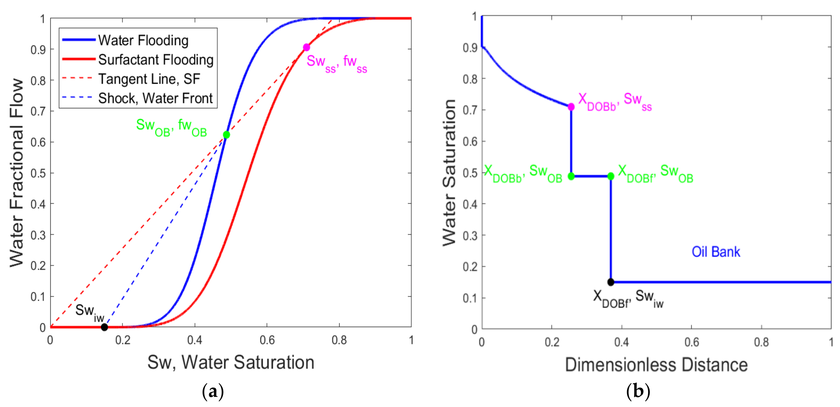
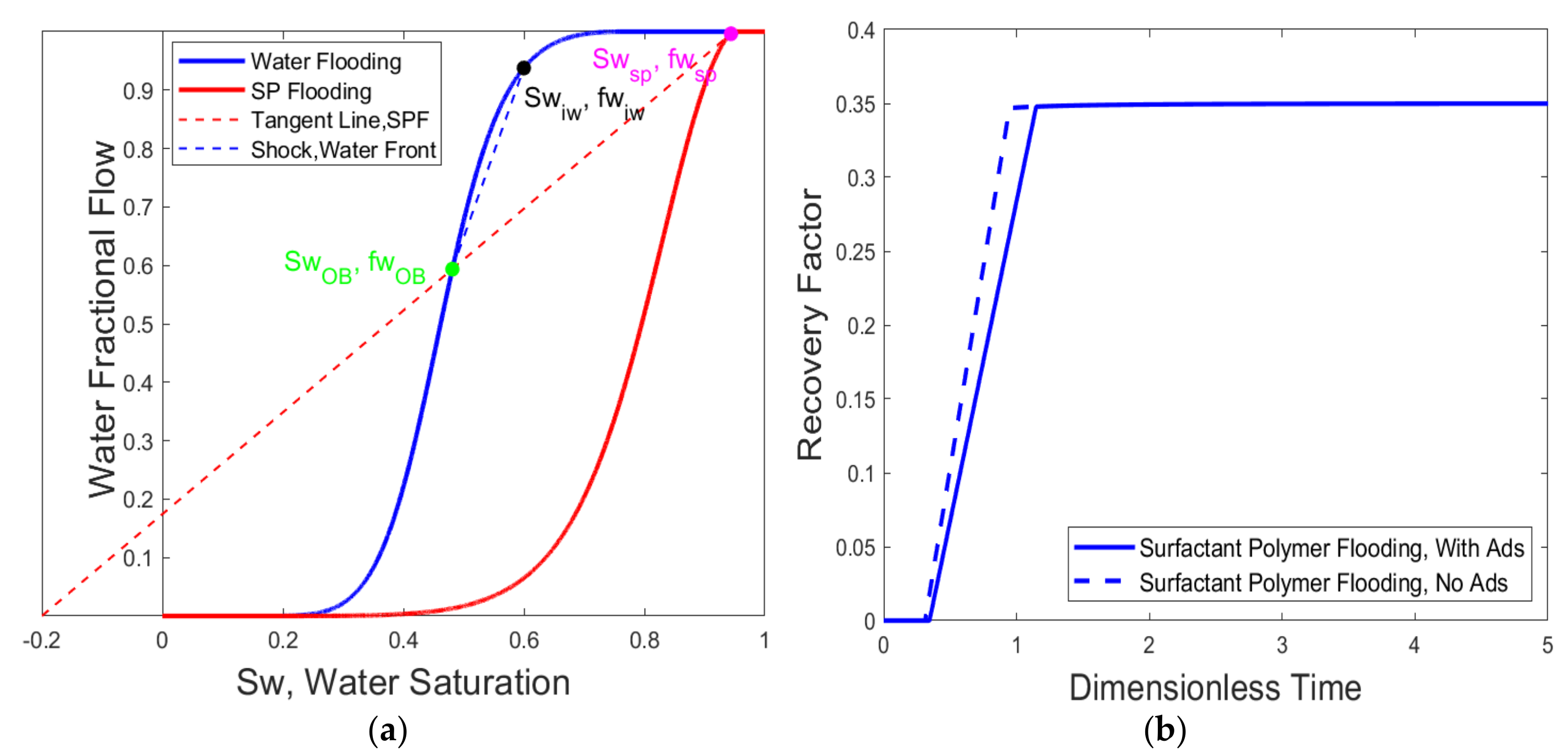
Figure 7.
(a) Water–oil relative permeability curves in the absence and presence of surfactant; and (b) Fractional flow curves in the absence and presence of surfactant (no adsorption, no partition) and construction of the respective shock front for water flooding and surfactant flooding.
Figure 7.
(a) Water–oil relative permeability curves in the absence and presence of surfactant; and (b) Fractional flow curves in the absence and presence of surfactant (no adsorption, no partition) and construction of the respective shock front for water flooding and surfactant flooding.
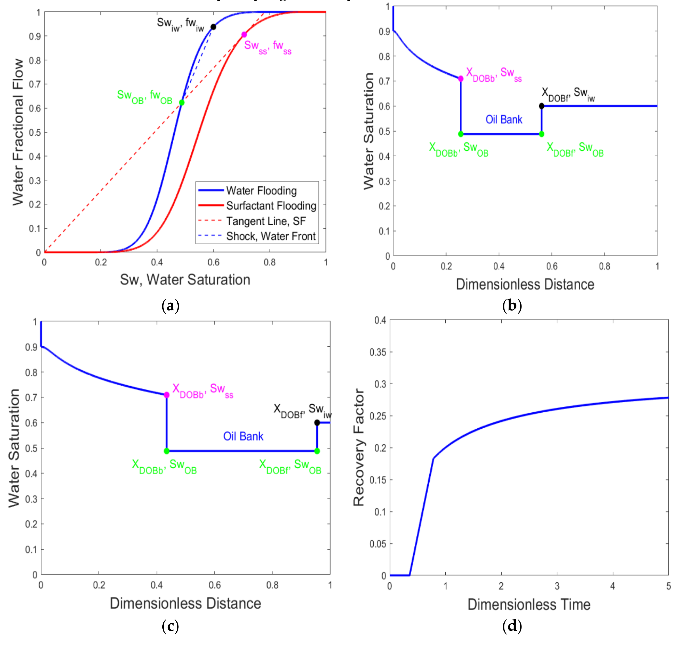
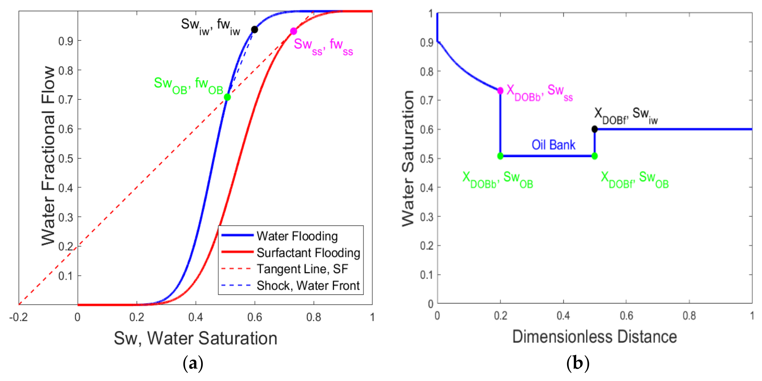
Figure 8.
(a) Construction of shock front; (b) water saturation profile at tD = 0.20 PV; (c) water saturation profile at tD = 0.34 PV; and (d) cumulative oil recovery during tertiary continuous surfactant flooding, no adsorption, no partition.
Figure 8.
(a) Construction of shock front; (b) water saturation profile at tD = 0.20 PV; (c) water saturation profile at tD = 0.34 PV; and (d) cumulative oil recovery during tertiary continuous surfactant flooding, no adsorption, no partition.
Figure 9.
(a) Construction of shock front; and (b) water saturation profile at tD = 0.2 PV during continuous surfactant injection, with adsorption, Di = 0.20 PV, no partition. PV: pore volume.
Figure 9.
(a) Construction of shock front; and (b) water saturation profile at tD = 0.2 PV during continuous surfactant injection, with adsorption, Di = 0.20 PV, no partition. PV: pore volume.
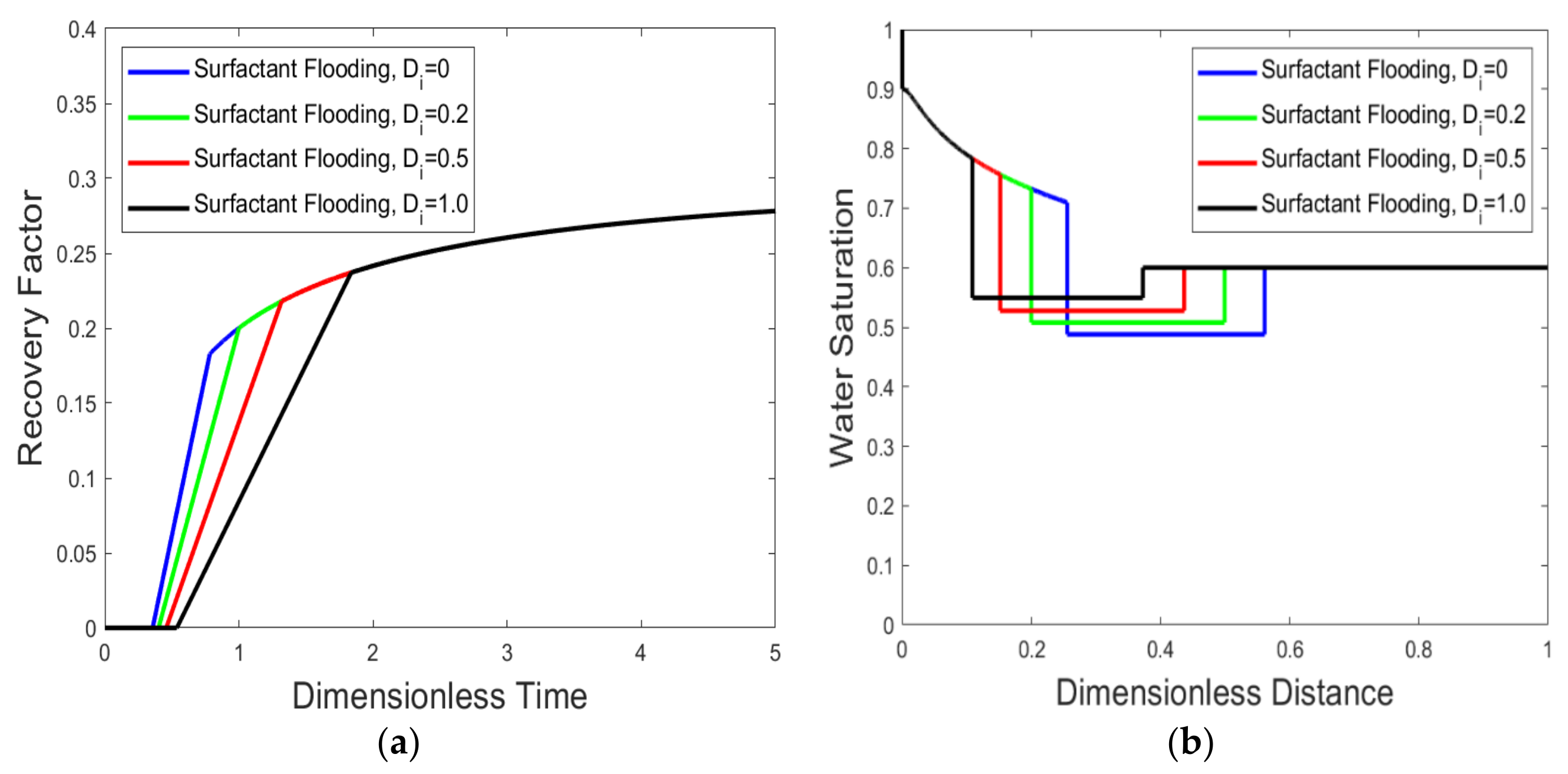
Figure 10.
(a) Incremental oil recovery by surfactant flooding as a function of retardation factor; and (b) saturation profile at tD = 0.2 PV for different retardation factors.
Figure 10.
(a) Incremental oil recovery by surfactant flooding as a function of retardation factor; and (b) saturation profile at tD = 0.2 PV for different retardation factors.
Figure 11.
(a) Incremental oil recovery by surfactant flooding as a function of retardation factor; and (b) saturation profile at tD = 0.2 PV for different retardation factor.
Figure 11.
(a) Incremental oil recovery by surfactant flooding as a function of retardation factor; and (b) saturation profile at tD = 0.2 PV for different retardation factor.
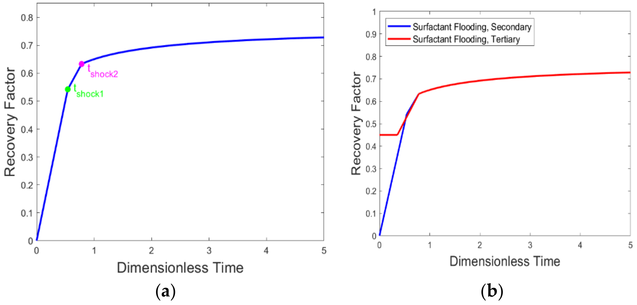
Figure 12.
(a) Cumulative oil recovery history during the secondary recovery process and (b) comparison of cumulative oil recovery during the secondary and tertiary processes for continuous surfactant injection with no surfactant adsorption and no surfactant partition.
Figure 12.
(a) Cumulative oil recovery history during the secondary recovery process and (b) comparison of cumulative oil recovery during the secondary and tertiary processes for continuous surfactant injection with no surfactant adsorption and no surfactant partition.
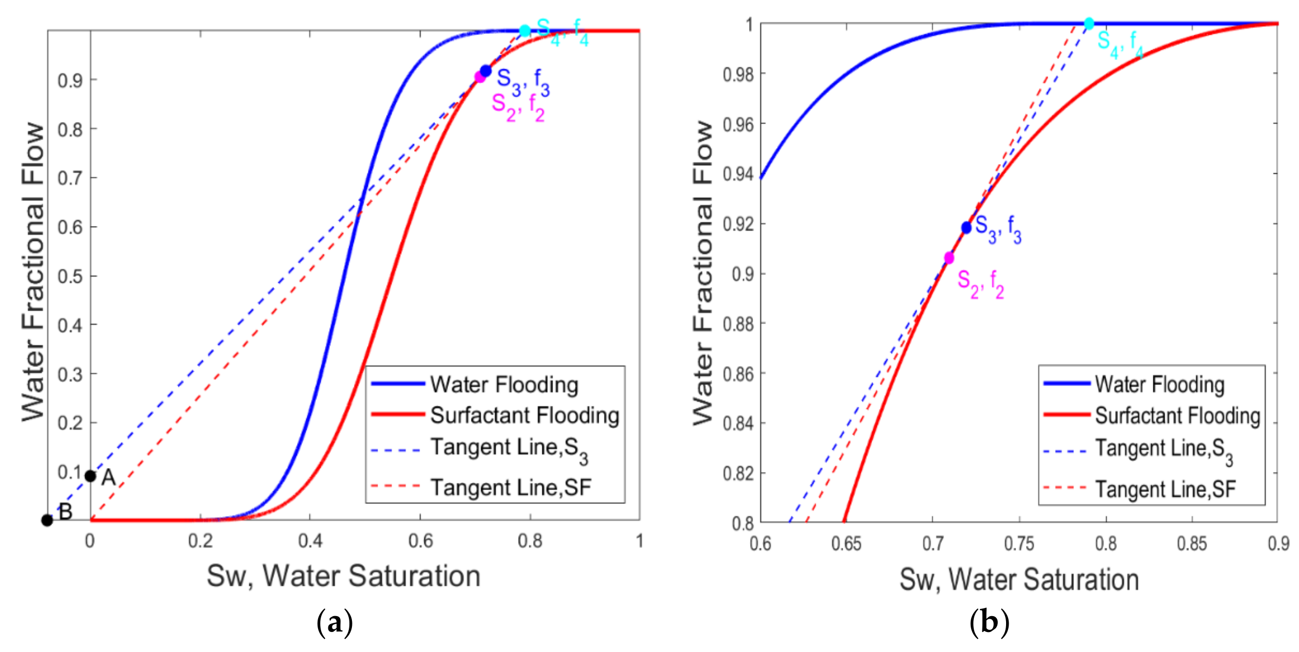
Figure 13.
(a) Determination of the shock front during surfactant slug injection; (b) Magnification of figure (a) for determining shock front location, = 0.30 PV, = 3.32 PV.
Figure 13.
(a) Determination of the shock front during surfactant slug injection; (b) Magnification of figure (a) for determining shock front location, = 0.30 PV, = 3.32 PV.
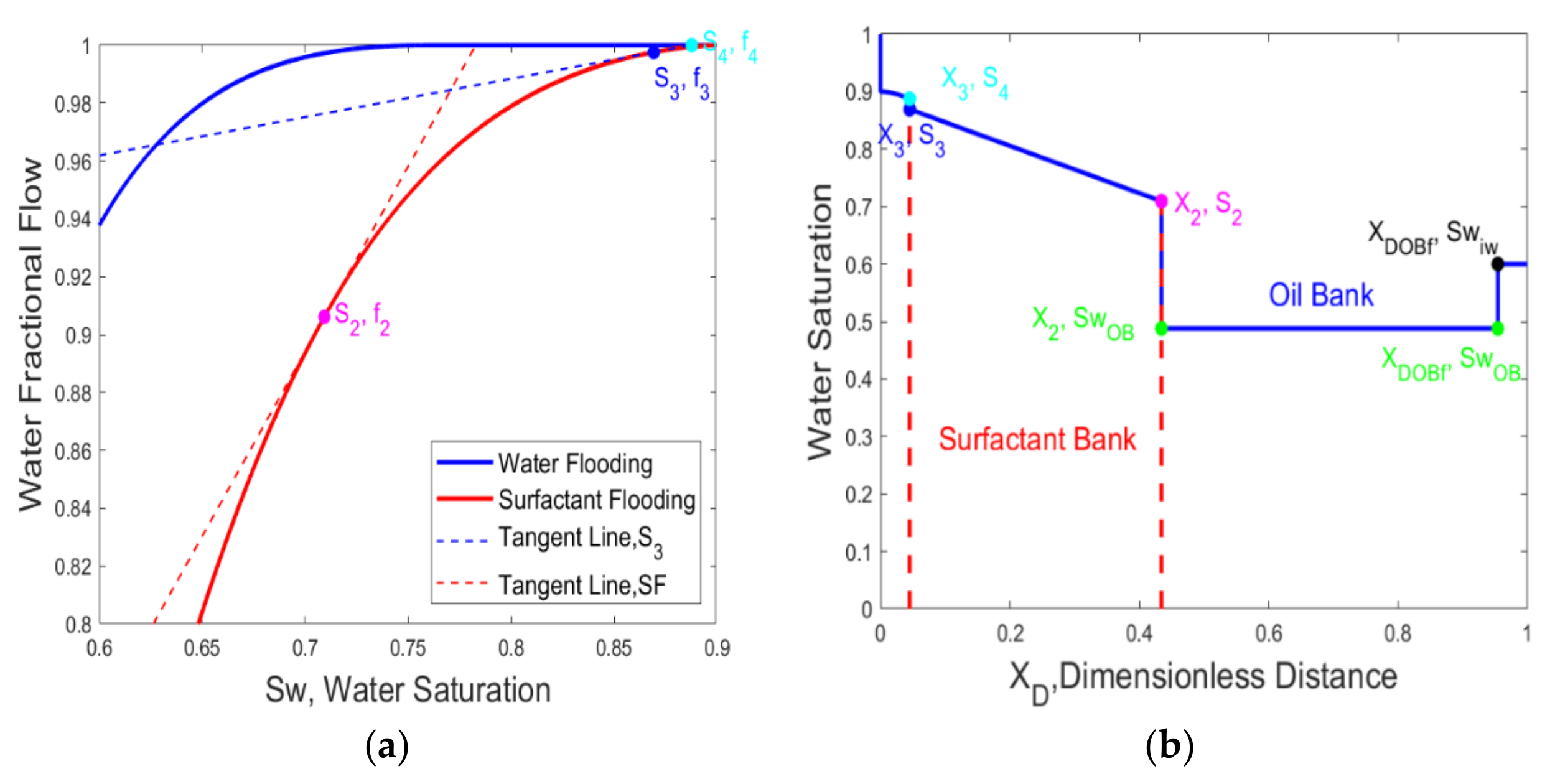
Figure 14.
(a) Determination of the shock front during surfactant slug injection; and (b) water saturation profile and oil bank at = 0.34 PV, surfactant slug size = 0.30 PV.
Figure 14.
(a) Determination of the shock front during surfactant slug injection; and (b) water saturation profile and oil bank at = 0.34 PV, surfactant slug size = 0.30 PV.
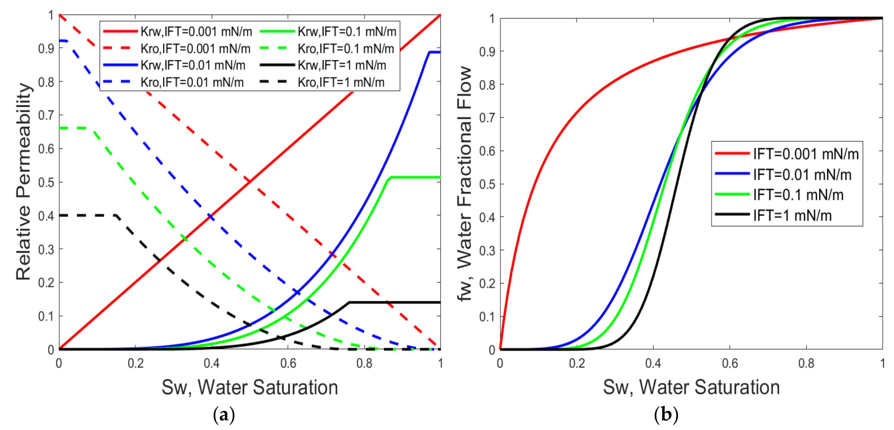
Figure 15.
(a) Water/oil relative permeability; and (b) water fractional flow as a function of water saturation and interfacial tension (IFT).
Figure 15.
(a) Water/oil relative permeability; and (b) water fractional flow as a function of water saturation and interfacial tension (IFT).
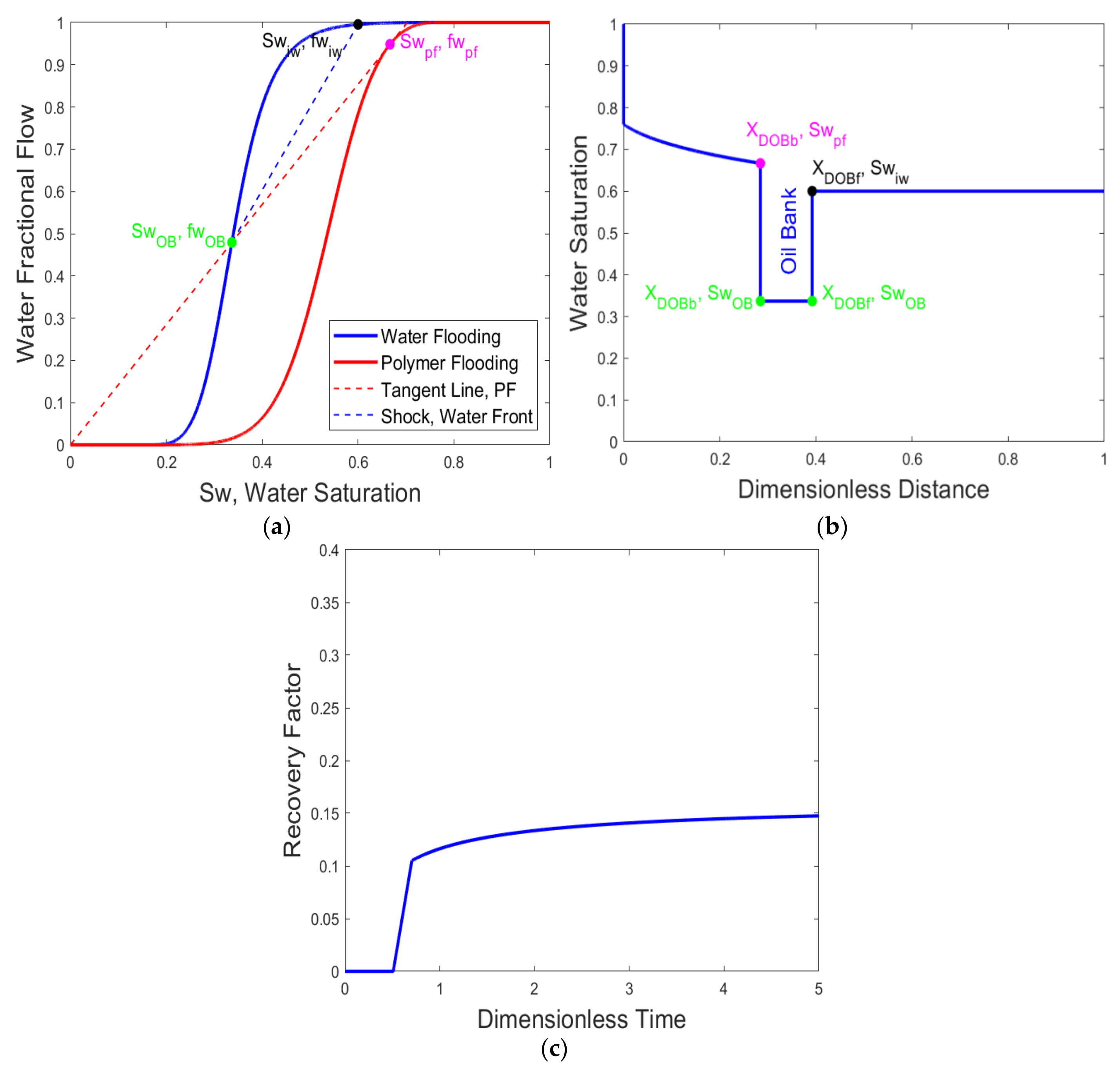
Figure 16.
(a) Construction of shock front; (b) Water saturation profile at tD = 0.20 PV; and (c) Cumulative oil recovery for tertiary polymer flooding, continuous injection, no polymer retention.
Figure 16.
(a) Construction of shock front; (b) Water saturation profile at tD = 0.20 PV; and (c) Cumulative oil recovery for tertiary polymer flooding, continuous injection, no polymer retention.
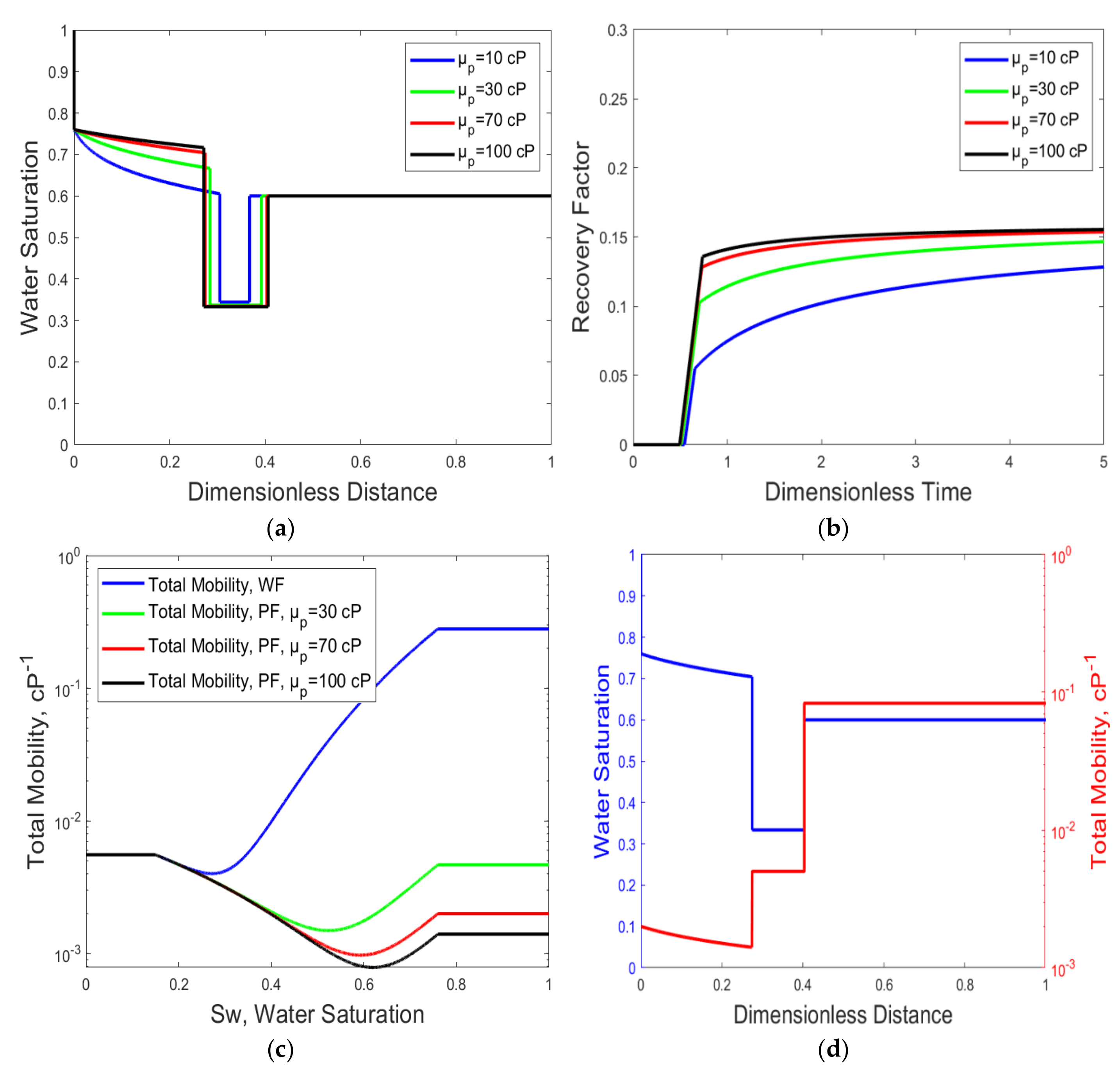
Figure 17.
(a) Comparison of shock front for water flooding and polymer flooding; (b) Incremental oil recovery history during continuous tertiary polymer flooding; (c) Total mobility as a function of water saturation for different polymer viscosity; and (d) Total mobility calculated during polymer flooding, tD = 0.20 PV, µp = 70 cP, µo = 72 cP.
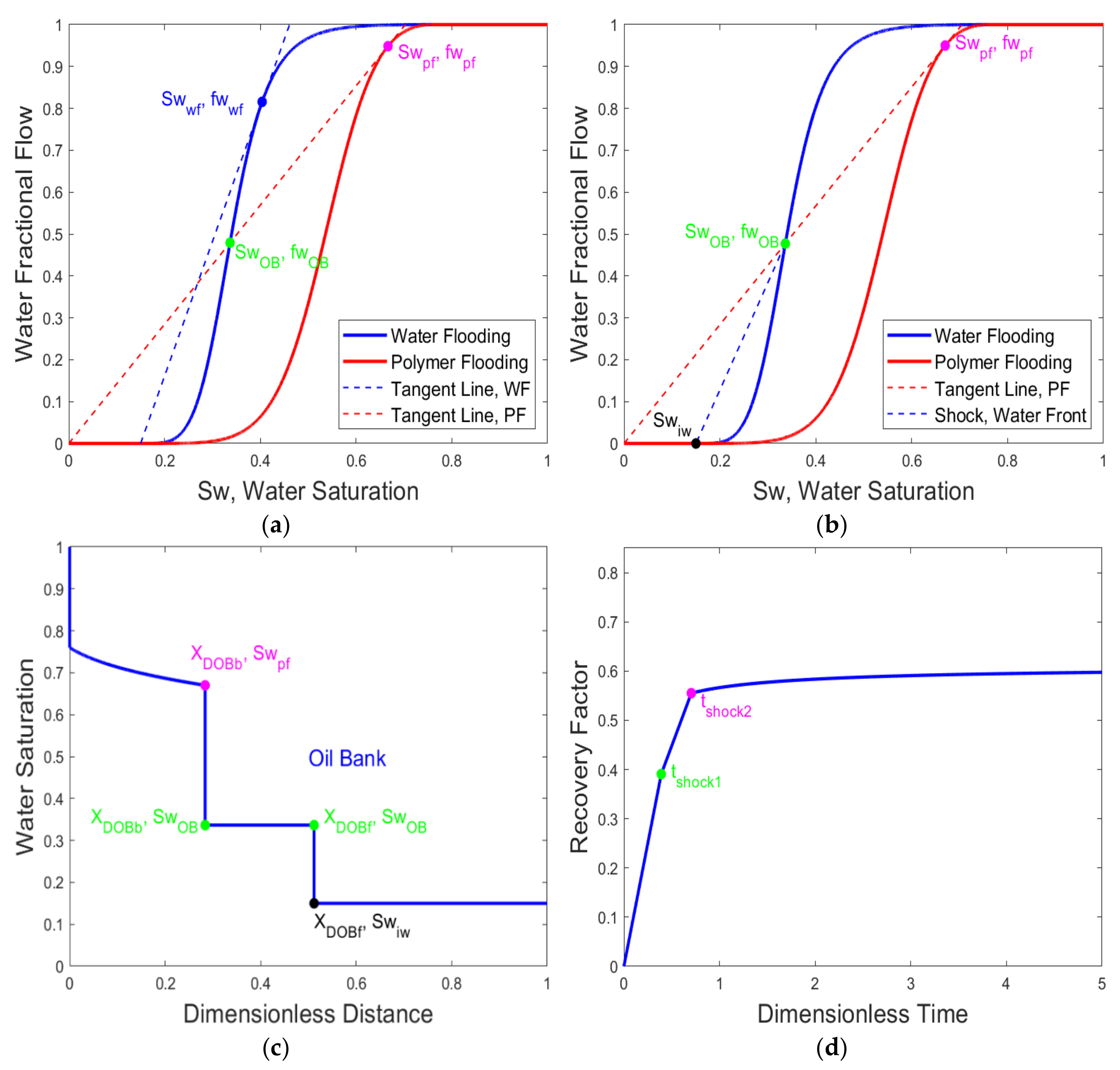
Figure 18.
(a) Comparison of shock front for water flooding and polymer flooding; (b) Construction of shock front during secondary recovery by polymer flooding; (c) Water saturation profile at tD = 0.2 PV during continuous polymer injection; and (d) Cumulative oil recovery history during secondary recovery by polymer flooding.
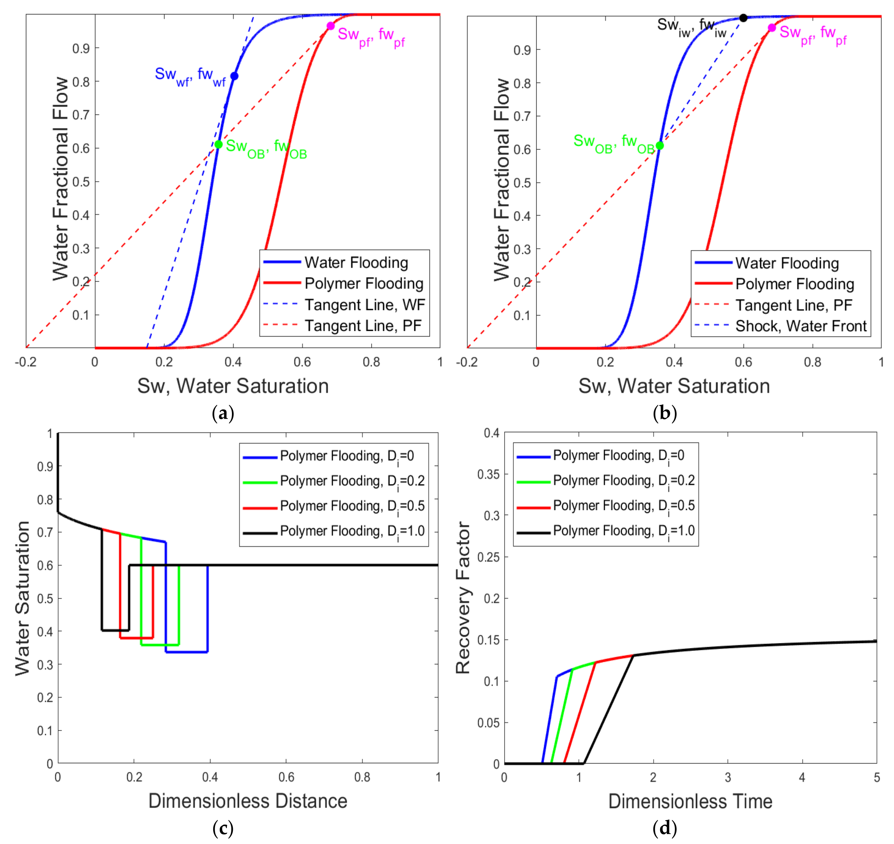
Figure 19.
(a) Comparison of shock front for water flooding and polymer flooding; (b) Construction of shock front during tertiary polymer flooding; (c) Saturation profile at tD = 0.20 PV during tertiary polymer flooding; and (d) Incremental oil recovery history during tertiary polymer flooding at a different retardation factor.
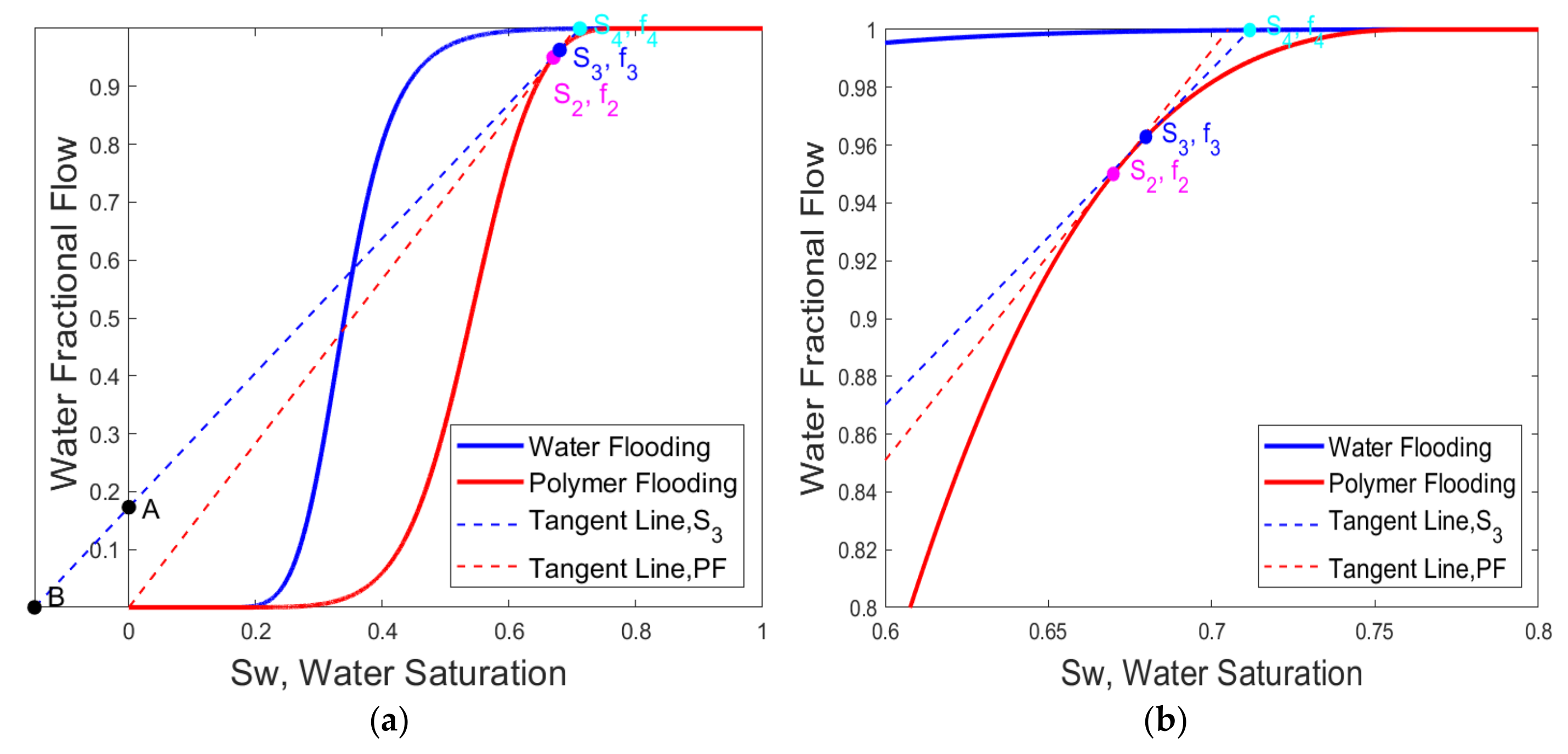
Figure 20.
(a) Determination of the shock front during polymer slug injection; (b) Magnification of figure (a) for determining shock front location, = 0.30 PV, = 1.74 PV.
Figure 20.
(a) Determination of the shock front during polymer slug injection; (b) Magnification of figure (a) for determining shock front location, = 0.30 PV, = 1.74 PV.
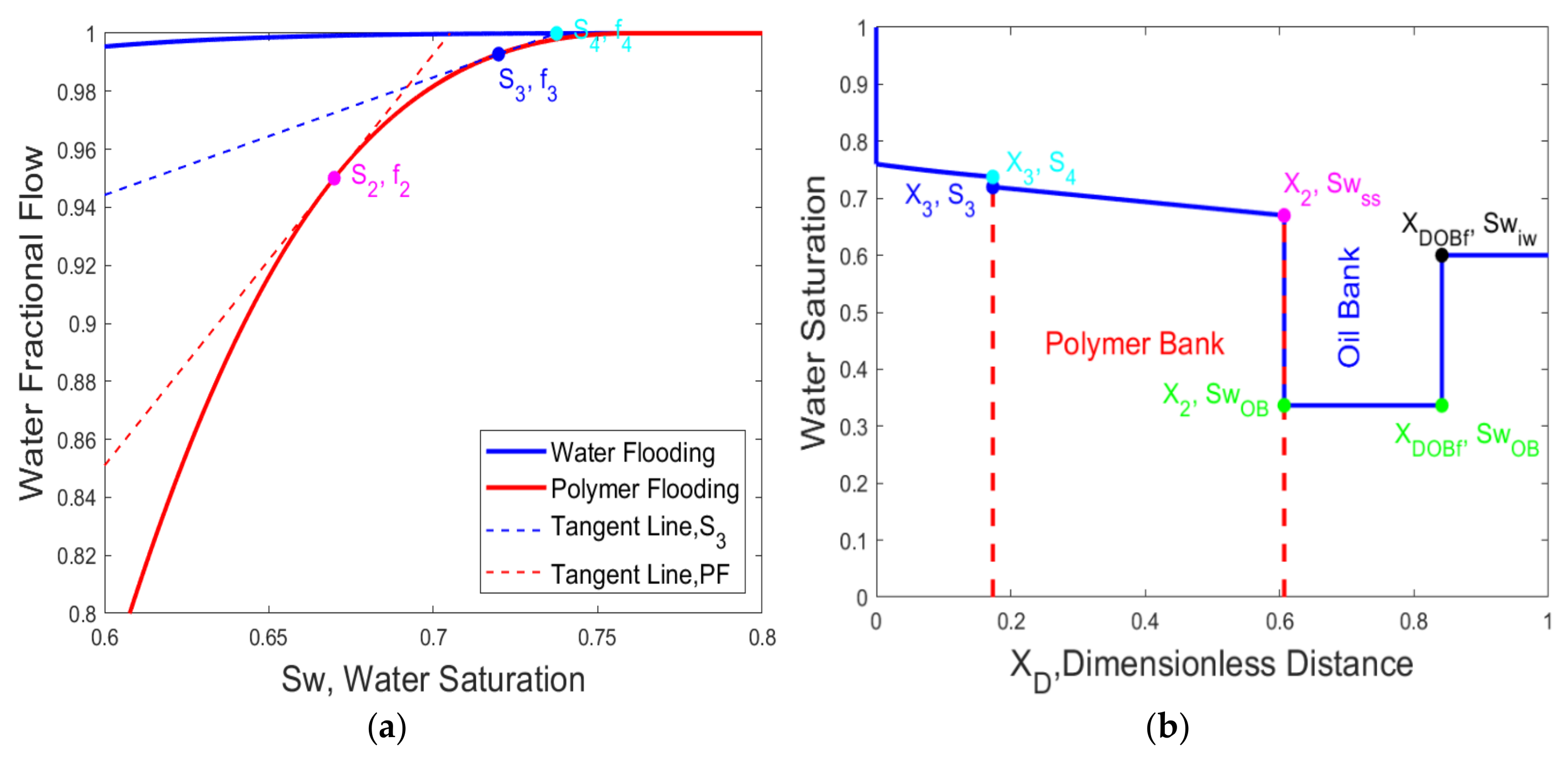
Figure 21.
(a) Determination of the shock front during polymer slug injection; (b) Profile of water saturation and oil bank at = 0.30 PV, = 0.43 PV.
Figure 21.
(a) Determination of the shock front during polymer slug injection; (b) Profile of water saturation and oil bank at = 0.30 PV, = 0.43 PV.
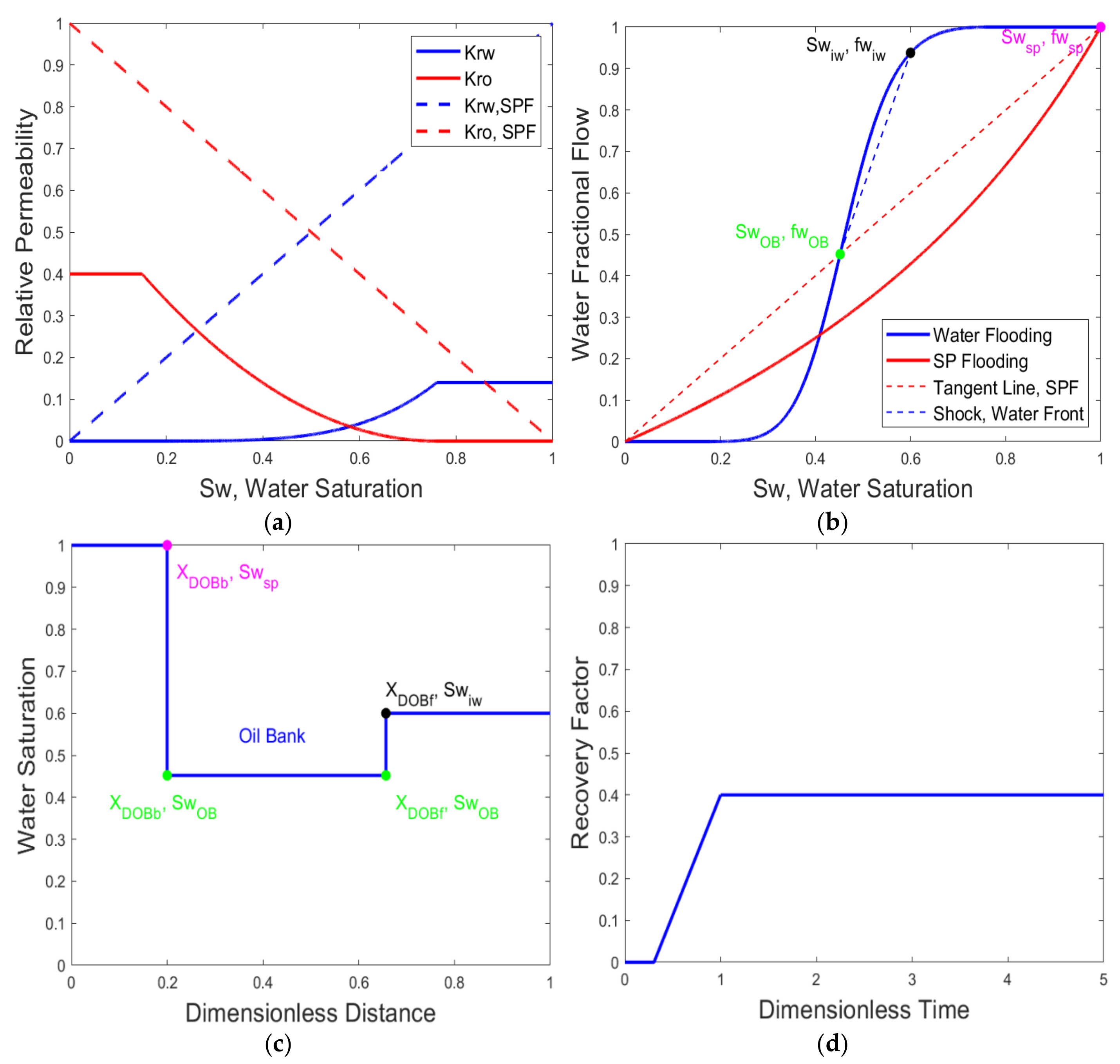
Figure 22.
(a) Water–oil two-phase relative permeability for water flooding and surfactant/polymer (SP) flooding; (b) Construction of shock front for water flooding and SP flooding; (c) Construction of shock front for continuous tertiary SP flooding, no adsorption; and (d) Water saturation profile at tD = 0.20 PV during SP flooding, no adsorption.
Figure 23.
(a) Construction of shock front for water flooding and surfactant/polymer flooding, with adsorption; and (b) Comparison of cumulative oil recovery during SP flooding, between no adsorption and Di = 0.2.
Figure 23.
(a) Construction of shock front for water flooding and surfactant/polymer flooding, with adsorption; and (b) Comparison of cumulative oil recovery during SP flooding, between no adsorption and Di = 0.2.
Figure 24.
(a) Water–oil two-phase relative permeability for water flooding and piston-like displacement; (b) Construction of shock front for water flooding and piston displacement; (c) Water saturation profile at tD = 0.2 PV for piston-like SP flooding; and (d) Cumulative oil recovery during piston-like SP flooding.
Table 1.
Review of literatures about CEOR modeling using fractional flow.
Table 1.
Review of literatures about CEOR modeling using fractional flow.
| References | Polymer Flooding | Surfactant Flooding | Surfactant Polymer Flooding |
|---|
| Lake, 2014 [3] | √ | √ | √ |
| Juárez, 2019 [19] | √ | | |
| Koh, 2018 [20] | √ | | |
| Qi, 2018 [21] | √ | | |
| Pope, 1980 [31] | √ | √ | √ |
| Larson, 1976 [32] | | √ | |
| Farajzadeh, 2019 [33] | √ | √ | √ |
| Rossen, 2011 [41] | √ | | |
| Sun, 2019 [42] | √ | | |
Table 2.
Corey model parameters for water–oil two-phase relative permeability.
Table 2.
Corey model parameters for water–oil two-phase relative permeability.
| Water–Oil Two-Phase Relative Permeability |
|---|
| | | | | | | |
|---|
| 0.14 | 0.40 | 0.15 | 0.24 | 4 | 2 | 0.5 | 72 |
Table 3.
Corey model parameters for water–oil two-phase relative permeability in the presence and absence of surfactant.
Table 3.
Corey model parameters for water–oil two-phase relative permeability in the presence and absence of surfactant.
| Water–Oil Two-Phase Relative Permeability in the Absence of Surfactant |
|---|
| | | | | | | |
| 0.14 | 0.40 | 0.15 | 0.24 | 4 | 2 | 0.5 | 5 |
| Water–Oil Two-Phase Relative Permeability in the Presence of Surfactant |
| | | | | | | |
| 0.40 | 1.00 | 0.15 | 0.10 | 4.0 | 1.5 | 0.5 | 5 |
Table 4.
Corey model parameters for water–oil two-phase relative permeability in the presence and absence of surfactant and polymer.
Table 4.
Corey model parameters for water–oil two-phase relative permeability in the presence and absence of surfactant and polymer.
| Water–Oil Two-Phase Relative Permeability in the Absence of Surfactant/Polymer |
|---|
| | | | | | | |
| 0.14 | 0.40 | 0.15 | 0.24 | 4 | 2 | 0.5 | 5 |
| Water–Oil Two-Phase Relative Permeability in the Presence of Surfactant/Polymer |
| | | | | | | |
| 0.40 | 1.00 | 0.15 | 0.05 | 4.0 | 1.5 | 10 | 5 |
Table 5.
Corey model parameters for water flooding and piston-like displacement in the presence of surfactant/polymer.
Table 5.
Corey model parameters for water flooding and piston-like displacement in the presence of surfactant/polymer.
| Water–Oil Two-Phase Relative Permeability for Water Flooding |
|---|
| | | | | | | |
| 0.14 | 0.40 | 0.15 | 0.24 | 4 | 2 | 0.5 | 5 |
| Water–Oil Relative Permeability for Piston-Like SP Flooding |
| | | | | | | |
| 1.00 | 1.00 | 0.00 | 0.00 | 1.0 | 1.0 | 10 | 5 |


