Approximate Analytical Periodic Solutions to the Restricted Three-Body Problem with Perturbation, Oblateness, Radiation and Varying Mass


1
School of Mathematical Science, Yangzhou University, Yangzhou 225002, China
2
Departament de Matemàtiques, Universitat Autònoma de Barcelona, 08193 Bellaterra, Barcelona, Catalonia, Spain
*
Author to whom correspondence should be addressed.
Universe 2020, 6(8), 110; https://doi.org/10.3390/universe6080110
Submission received: 17 June 2020
/
Revised: 31 July 2020
/
Accepted: 2 August 2020
/
Published: 4 August 2020
(This article belongs to the Section Planetary Sciences)
Abstract
:Against the background of a restricted three-body problem consisting of a supergiant eclipsing binary system, the two primaries are composed of a pair of bright oblate stars whose mass changes with time. The zero-velocity surface and curve of the problem are numerically studied to describe the third body’s motion area, and the corresponding five libration points are obtained. Moreover, the effect of small perturbations, Coriolis and centrifugal forces, radiative pressure, and the oblateness and mass parameters of the two primaries on the third body’s dynamic behavior is discussed through the bifurcation diagram. Furthermore, the second- and third-order approximate analytical periodic solutions around the collinear solution point in two-dimensional plane and three-dimensional spaces are presented by using the Lindstedt-Poincaré perturbation method.
1. Introduction
It is well known that Newton’s famous proposition “Principle” took a decisive step in our understanding of the universe. The origin of the universe is inseparable from the three-body dynamics, which has always existed since the universe’s birth. It can be said that there are no three-body dynamics; it is impossible to create a universe [1]. The three-body interactions in the early universe help people understand the black hole MACHO (abbreviation of MAssive Compact Halo Object) binary formation and the detectability of gravitational waves in black hole MACHO binaries coalesce [2,3]. In the theoretical framework of scalar-tensor gravitation, Zhou et al. [4] found that there is a collinear solution to the three-body problem in the presence of a scalar field, and studied the effect of the scalar field on this solution and the positions of Lagrange points through numerical examples. For the three-body problem in the spherical universe, their perturbation theory analysis showed that the rate of precession of two small and nearly circular solutions of identical particles is proportional to the square root of their initial distance and inversely proportional to the square of the radius of the universe [5]. In addition, the three-body problem is also widely used in the evolution of binary systems [6] and the dynamic analysis of binary asteroids [7,8], as well as other fields in the universe such as dark matter, galaxies, GW170817 (GW is short for gravitational wave), and Mukhanov-Sasaki Hamiltonian dynamics, and so forth (see References [9,10,11,12,13] for more information).
The mathematician Poincaré believed periodic solutions to be the unique avenue for solving the three-body problem. He stated that “what makes these solutions so precious to us, is that they are, so to say, the only opening through which we can try to enter a place.” There is too much literature in this area, mainly involving three aspects—qualitative analysis, approximate quantitative solution, and computer-aided numerical simulation (see References [14,15,16,17,18,19,20,21,22,23,24,25,26,27,28,29,30,31,32], and the references therein).
When considering multiple perturbation factors, Singh et al. did a great deal of work on the libration points and their stability of various restricted three-body models (see References [33,34,35,36,37,38,39,40,41]). These factors mainly include the oblateness of the primaries [35,36,37,38,40,41], the oblateness of the third body [37], and the small perturbation in centrifugal force and Coriolis force [35,36,37,38,39,40,41], the radiation pressure of the primaries [33,34,35,36,37,38,39,40,41], the changing mass of the primaries over time based on the Meshcherskii law [34,35,36], the changing mass of the third body governed by Jeans law [42], the triaxiality of the primaries [39]. Basic references on oblateness, Coriolis and centrifugal forces, and radiation pressure can be found in References [43,44,45,46,47].
In addition, some other researchers also discussed the periodic solutions and libration points of the restricted three-body problem (R3BP) under specific perturbations. For example, Abdullah et al. [48] investigated the locations and stability of libration points in the circular R3BP with Coriolis and centrifugal forces under the assumption that the two primaries and the infinitesimal body with variable masses. Under the assumption that the more massive primary has triaxiality, Abouelmagd et al. [49] obtained the approximate periodic solution near the collinear libration point of R3BP to the second-order. Since the star’s isotropic radiation or absorption is one of the factors that cause the mass of the celestial bodies to change with time, Bekov [50] considered the R3BP of variable masses, in which the motion of the two primaries was determined by the Gylden-Meshcherskii problem and found the collinear solutions, as well as the spatial solution and its domains of existence. When the more extensive primary is an oblate sphere, Zotos [51] numerically studied the dynamic behavior of the circular R3BP under the initial conditions of the solution are bounded, escaping and collisional, and found that the oblateness factor has a significant influence on the characteristics of the solutions. Based on the model of the binary system proposed in Reference [39], Gao and Wang [6] continued to study the analytical approximate periodic solutions around the collinear libration points. They examined the influence of the small perturbation in Coriolis and centrifugal forces, the triaxiality, and radiation pressure of the primaries on the third body’s dynamic behavior through the bifurcation diagram.
In this paper, the effects of small perturbations, Coriolis and centrifugal forces, radiation pressure, and the oblateness and variable mass of the primaries on the third body’s dynamic behavior will be discussed numerically through bifurcation diagram in the context of an R3BP consisting of a supergiant eclipsing binary system. Here we take into account the oblateness, Coriolis and centrifugal forces together because the oblateness of the primaries will cause both Coriolis force and centrifugal force to increase (see References [52,53]). By Lindstedt-Poincaré perturbation method, the approximate analytical solutions of the perturbed third body in two and three dimensions near the collinear libration points will be obtained. This paper is organized as follows—the motion equations in an autonomous system will be given in Section 2. The geometry structure of the zero velocity surfaces and curves will be illustrated in Section 3. Moreover, the bifurcation diagrams of the different perturbation parameters will be shown in Section 4. Furthermore, the periodic planar and spatial solutions near the collinear libration points will be obtained by means of Lindstedt-Poincaré in Section 5. In the last Section 6, conclusions will be stated.
2. Equations of Motion
In a barycentric coordinate , consider that two oblate variable-mass radiating primaries move at an angular velocity in a circular orbit around their center of mass. The plane of motion of the primaries (located on the x-axis) coincides with the x-y plane. The third body of infinitesimal mass that moves under the gravity of the primaries but does not affect their motion, then the dynamic governing equations (see Reference [35] or Reference [36] for more details) can be written as follows
where () denotes the distance between the ith primary and the third body, and the two primaries are placed on and , respectively. For the distance r between the primaries, , , , , represents the mass of the ith primary, f is the gravitational constant. In addition, the parameters and stand for the radiation factor and the varying oblateness of the ith primary, respectively. The Coriolis force and centrifugal force satisfy , , here and are the corresponding small perturbations with values far less than 1. Furthermore, it can be followed from the reference [36] that the angular velocity holds the following expression
where is an arbitrary dimensionless constant of a particular integral in Gyldén-Meshcherskii problem (see References [54,55,56] for more information), it represents an arbitrary sum of the masses of the primaries, C is a constant of the area integral. Note that if the masses of the primaries are constant and the sum , then by unitizing the gravitational constant. In addition, if the distance r between the primaries is 1, and without considering the oblateness of the second primary, that is, . Then Equation (2) is simplified to , which is the same as the mean motion expression in Reference [47].
We now transform Equations (1) into the autonomous system by the Meshcherskii’s transformation (see Reference [35] or Reference [57])
where is the distance between the third body and the ith primary, , , and are constants, the unified Meshcherskii law
where , , are constants, and the particular solutions of Gyldén-Meshcherskii problem,
where is the distance between the two primaries at initial time. Applying transformation , here refers to the oblateness of the ith primary at initial time, and are the equatorial radii and the polar radii of the ith primary, respectively. Similarly, following Singh and Leke [35], unify the mass and distance at the initial time and introduce the mass parameter which satisfies , , stands for the ratio of the smaller mass to the total mass of the two primaries, then , . Therefore, we obtain
3. Zero Velocity Surfaces and Curves
The level surface of Equation (7) is an energy surface. The projection of this surface onto position space is named Hill’s region, and its boundary is the zero-velocity surface, on which the velocity of the third body is zero, so the third body can only move inside the zero-velocity surface. The intersection of this surface with the x-y plane is known as the zero-velocity curve. Note that Equation (7) admits a first integral
where C is the Jacobi constant and denotes the velocity of the relative motion. The geometric structure of in the two-dimensional plane and three-dimensional space is shown as a series of curves and surfaces for the different Jacobi constants C.
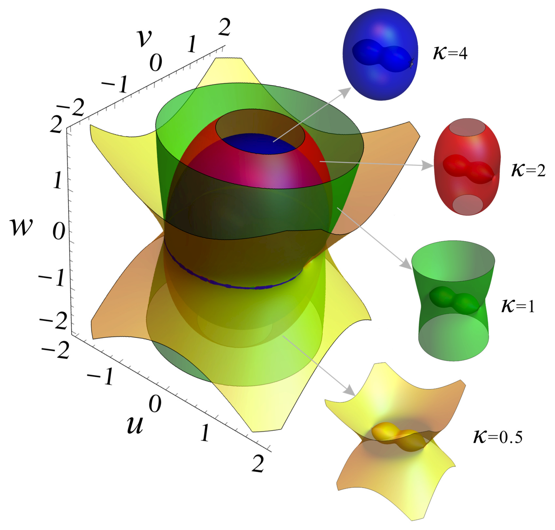
The zero-velocity surface (or curve) with perturbations helps us to analyze the third body’s dynamic behavior under the influence of a specific perturbation factor, which is different from that of classical R3BP. For example, when , and , the zero-velocity surface is different from the classic R3BP due to the presence of . For the parameter values presented in Table 1, Figure 1 shows the four zero-velocity surfaces when takes 0.5, 1, 2 and 4, respectively. It is easy to find that the structure of the zero-velocity surface of Equation (9) is more open as the value of becomes smaller and smaller. Because the geometry of the zero-velocity surface (or curve) will vary with the value of the Jacobi constant C and , we can numerically analyze the zero-velocity surface (or curve) and then find the libration points of Equation (7). Without loss of generality, now we only study the surfaces and curves for the case .
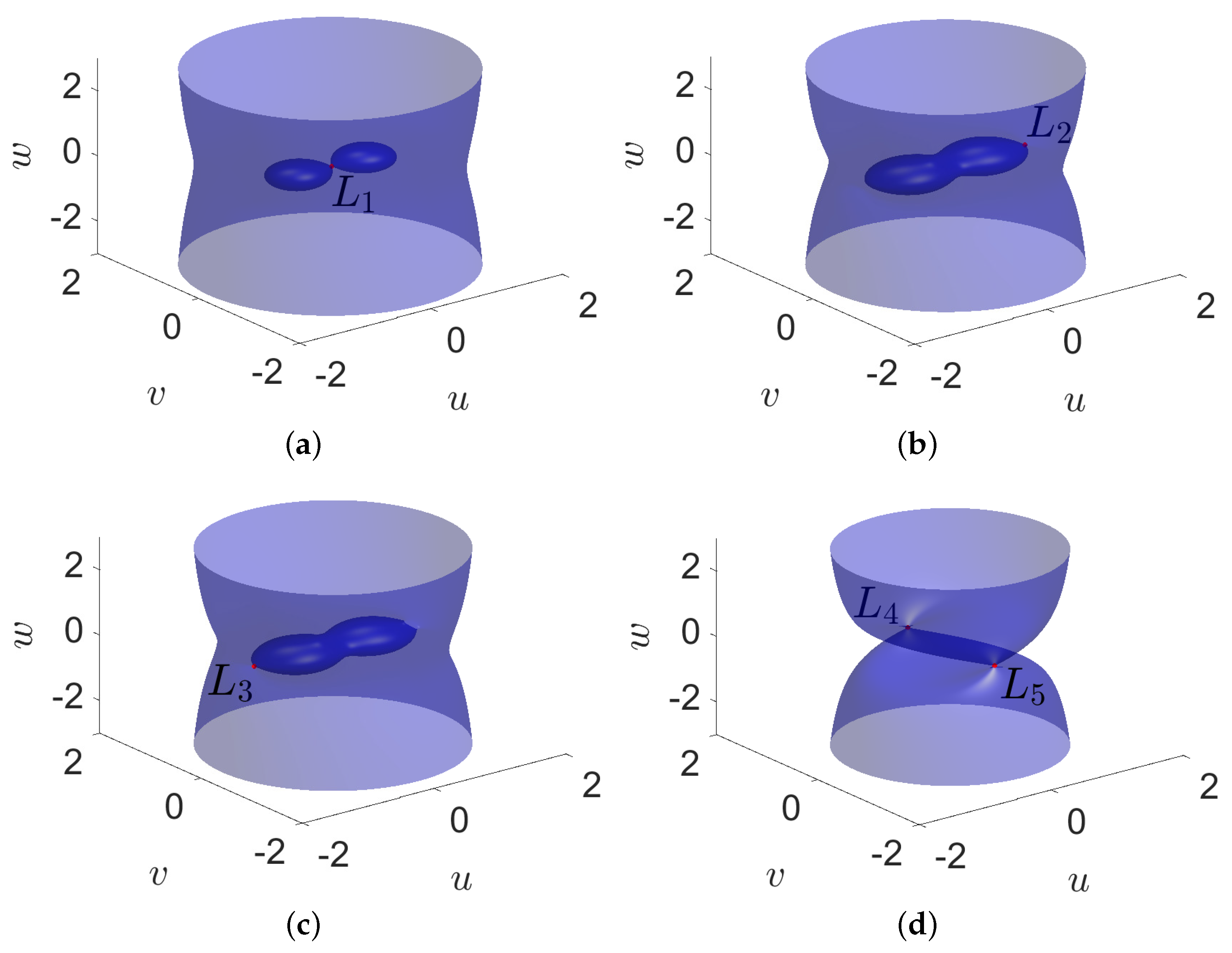
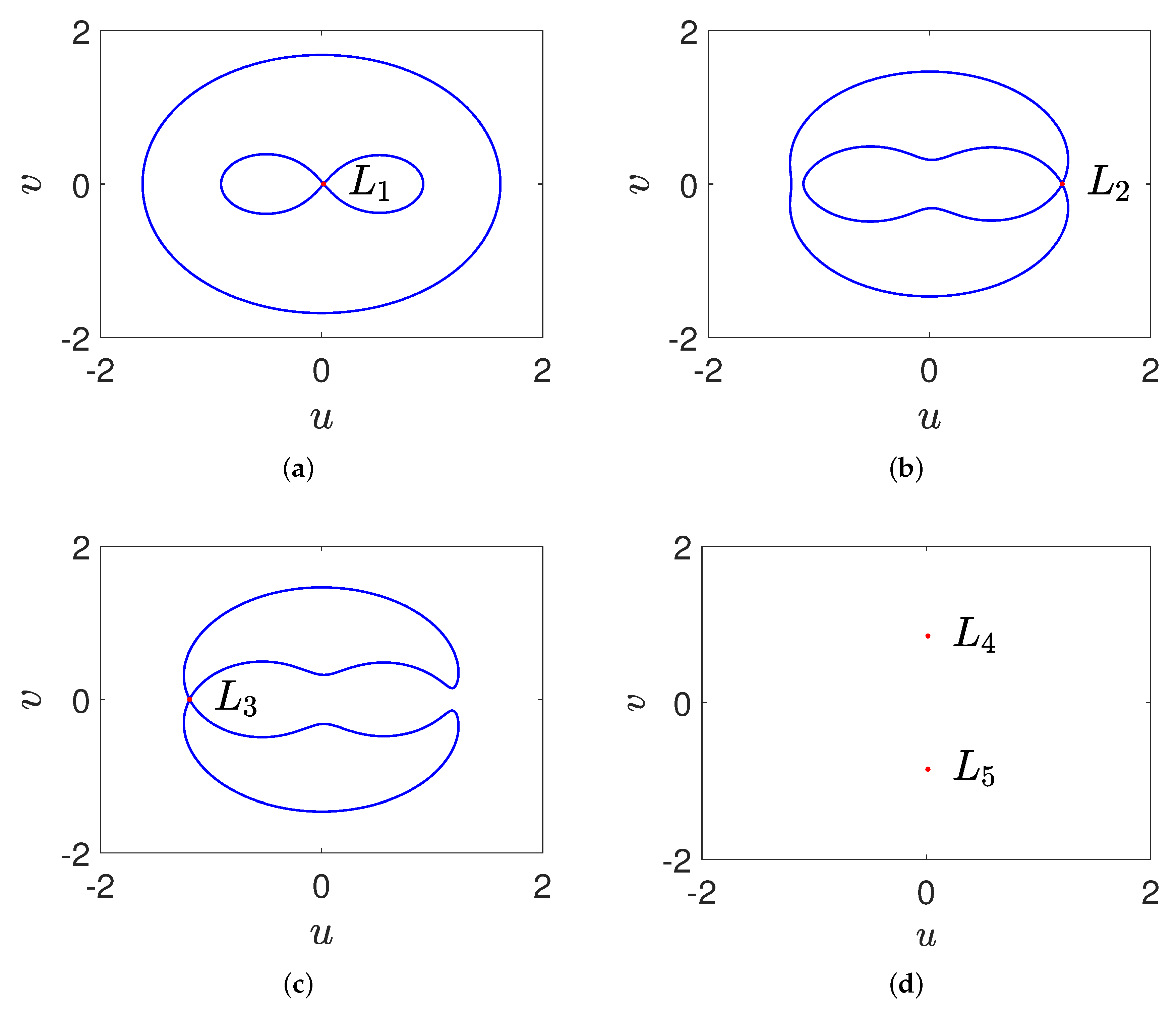
For , the forbidden region of the third body changes with the Jacobi constant C as shown in Figure 2 and Figure 3. With the decrease of C, five regular libration points , are discovered gradually and the forbidden region of motion of the third body is shrinking. More precisely, the third body can only fly in the two ellipsoidal areas around the two primaries when , and the two ellipsoidal motion areas are connected together through the “tangent point” (marked as librarian point ), and the third body can pass from one primary to the other through when , but it cannot fly out of these two ellipsoidal areas. When , the peanut-shaped flight area is connected to the outer space through a new “tangent point” , and when the value of C continues to decrease, the third body can only enter the outer space in this direction. When C drops to 3.57940, we will discover another new “tangent point” in the opposite direction, which is the libration point . At this time the third body can also fly from this direction to outer space when the value of C continues to decrease. For the Jacobi constant , the symmetrical libration points and appear at the same time. Now the third object can escape into outer space in any direction around the two primaries. Therefore, as a summary of Figure 2 and Figure 3, the corresponding five planar librations points can be identified as follows , , , , . Besides, there are several methods for determining the libration points. For example, the total number of collinear libration points for this problem can also be determined based on the theory of topological degree [58].
4. Bifurcation Analysis
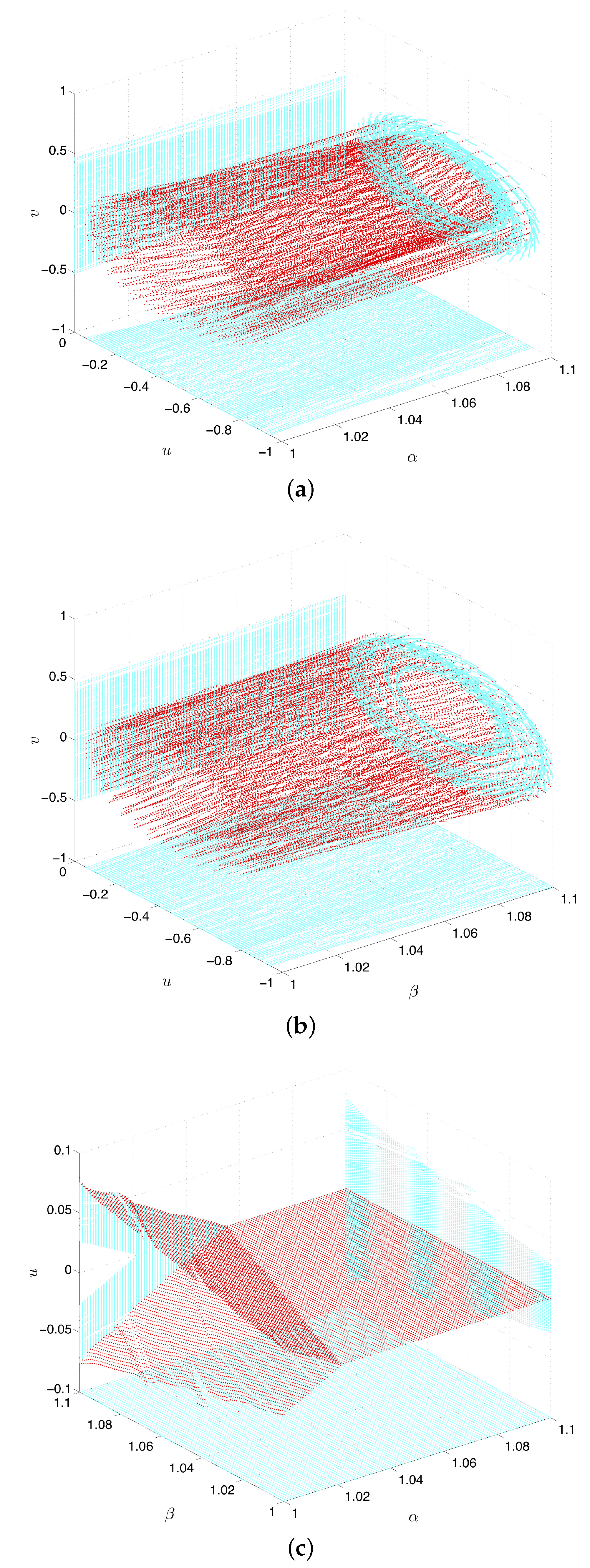
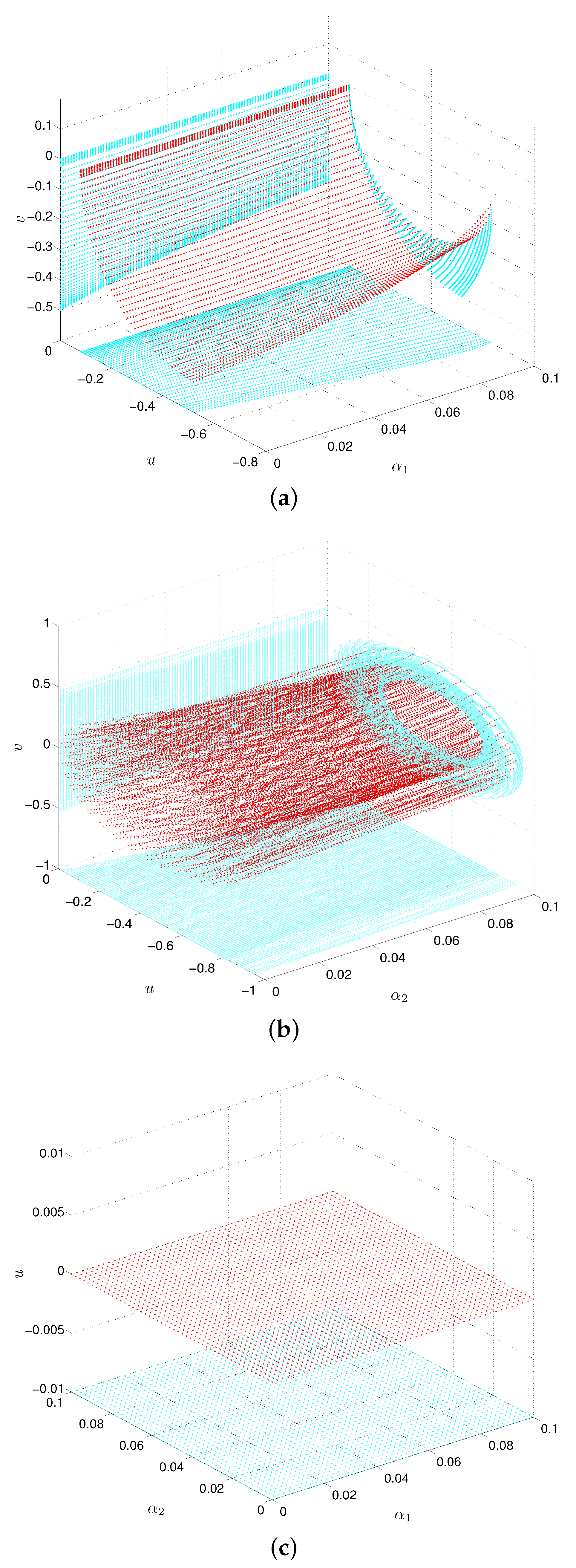
We note that the three-body problem has a high degree of complexity due to its dynamic equations’ extremely strong nonlinearity. Any subtle changes in different parameters may substantially change the third body’s dynamic behavior. Thus, we will analyze the effect of different perturbation parameters on the third body’s dynamic behavior through the bifurcation diagram. After a large number of numerical simulations, we select as the initial value of the iteration. Combining the conditions in Section 2, we restrict the Coriolis force and centrifugal force to [1, 1.1] in the --u frame, Figure 4a,b show the influence of the perturbation of and on the variables u-v, respectively, and reflect the corresponding chaotic characteristics. However, the joint perturbation of and shows that the amplitude of the third body in u direction no longer changes when (see Figure 4c).
Consider the perturbation range of the oblateness coefficients of the two primaries is . As shown in Figure 5a,b, as the oblateness coefficient of the first primary increases, the effect of this perturbation factor on the third body’s amplitude in u direction gradually increases, but the effect on the amplitude in v direction gradually decreases. When the oblateness coefficient of the second primary changes, the third body exhibits apparent chaotic behavior. However, the third body keeps moving periodically in u direction under the joint action of and (see Figure 5c). This indicates that the oblateness coefficients play a certain degree of “correction” to the two primaries’ dynamic behavior so that they can maintain regular motion as much as possible.
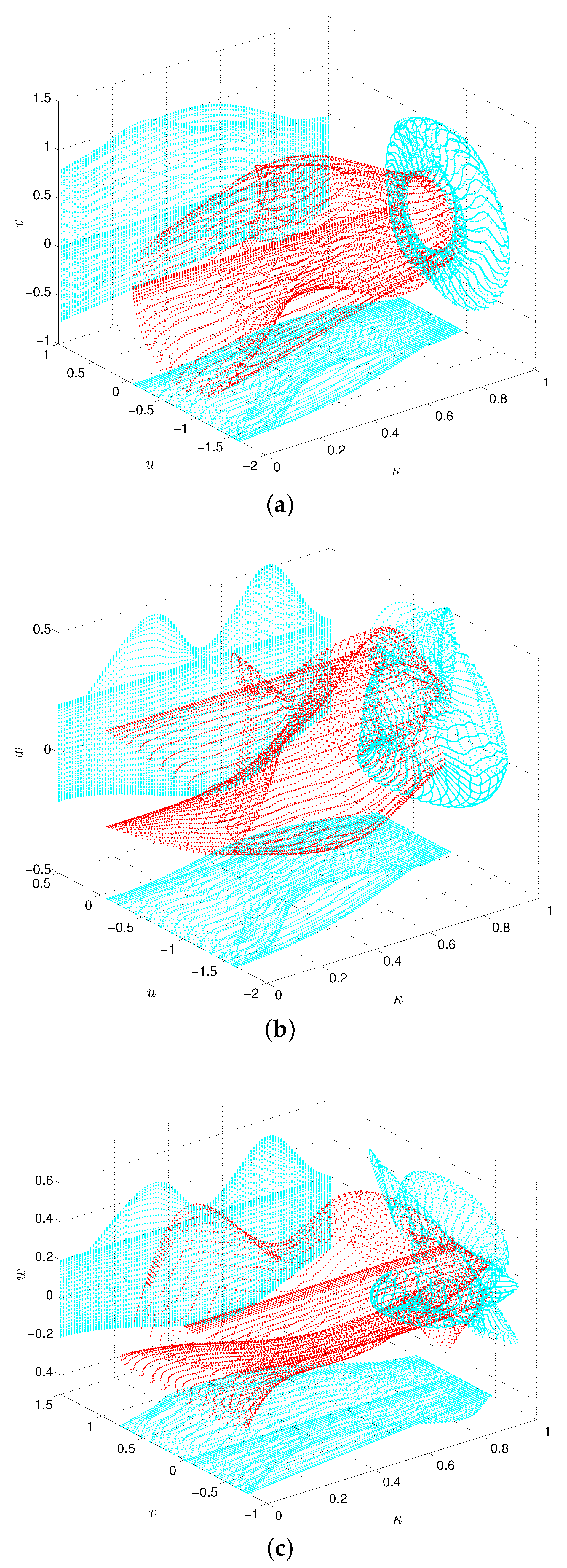
For the parameter , which represents the arbitrary sum of the primaries’ masses, we only show the bifurcation diagrams whose value is between 0 and 1. Figure 6a–c clearly show that no matter how the value of changes, it has a considerable influence on the third body’s dynamic behavior. The third body reflects the intricate, chaotic properties in the frames -u-v, -u-w, and -v-w. It is consistent with our common sense because the masses of the primaries are closely related to their gravitation, and this plays a significant role in determining the behavior of the third body in the sphere of gravity.
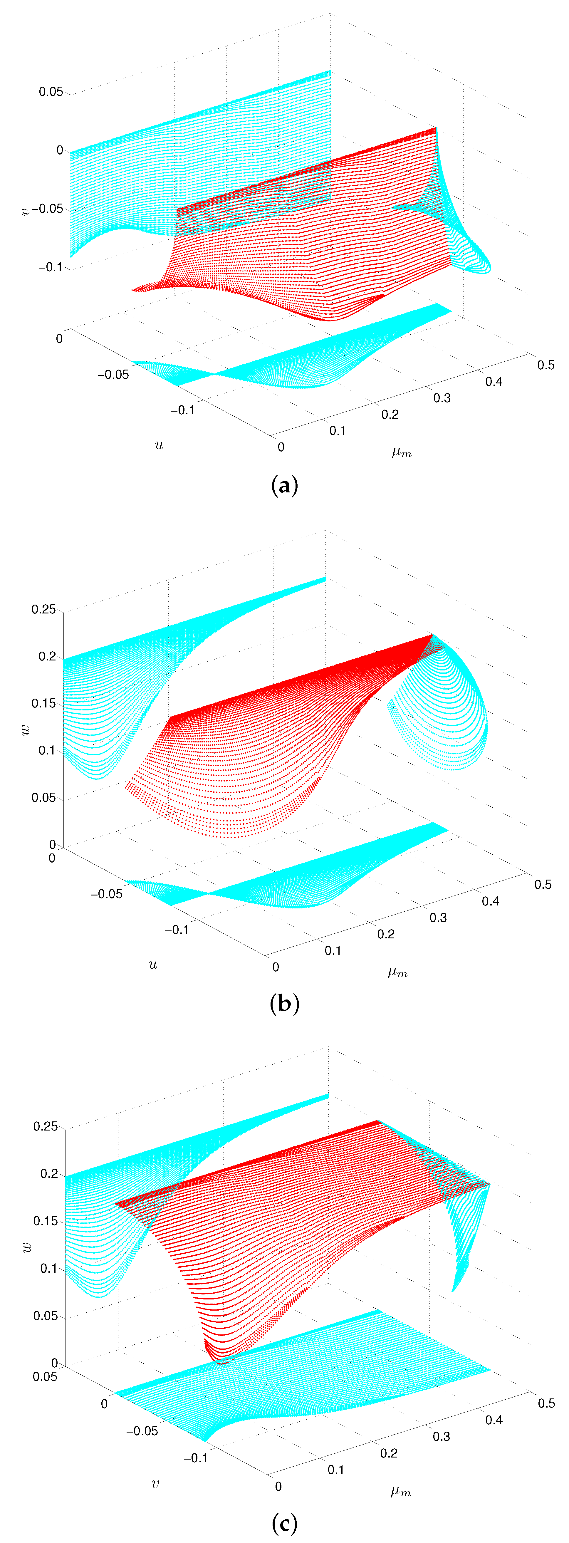
Next, we show the bifurcation diagrams of the mass parameter in the interval in Figure 7. It is easy to find that when ’s value is small, the mass of one primary is enormous compared to the other. It has a significant impact on the third body’s amplitude in the three directions of u, v, and w. When , the third body’s amplitude in u direction seems to be stable from its projection (see Figure 7a,b), but it is still apparent in the three-dimensional space. However, when the value of gradually increases, that is, the difference between the masses of the two primaries is getting smaller and smaller, its influence on the third body’s amplitude in the v direction is gradually more considerable than that in u and w directions (see Figure 7b,c).
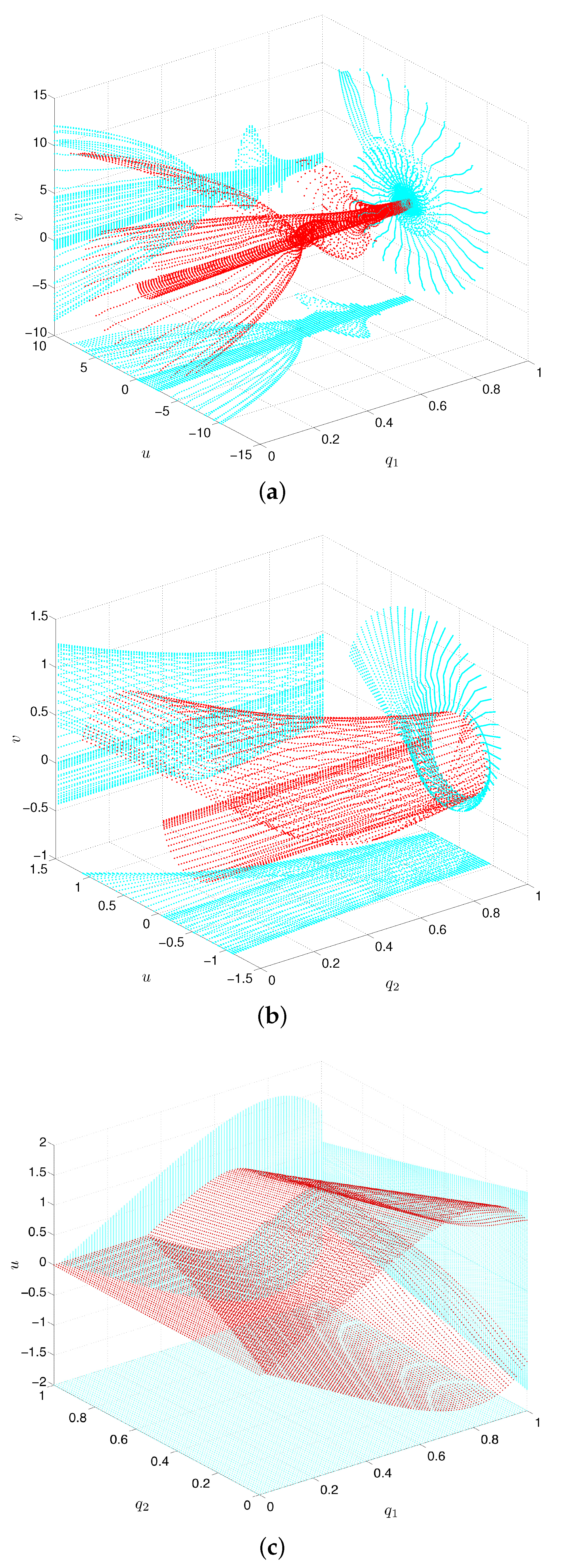
Similarly, we examine the effect of the radiation factors and on the third body’s dynamic behavior at the interval . Figure 8a,b demonstrate the influence of the radiation factors of the first and second primaries, respectively, and Figure 8c reflects the impact of the two radiation factors acting simultaneously. As shown in Figure 8a,b, the radiation factor or has almost the same influence on the third body’s movement in u and v directions. However, the influence of on the third body’s amplitude is greater than that of , especially when or . In contrast, the impact of is much more moderate. Figure 8c shows that when , regardless of how changes, the amplitude of the third body changes little in the u direction. In other words, the two radiations from the two primaries in the current state have almost little effect on the dynamic behavior of the third body in the u direction, which may be due to the weak radiation of the first primary. However, when , the third body’s amplitude has a significant change, even if is very small. When the value of is greater than 0.3434, the third body exhibits approximately symmetrical motion in a larger area under the joint action of and .
5. Periodic Solutions near the Collinear Libration Points
5.1. Expansion of Two-Dimensional Dynamic Equations
The third body’s equations of motion in the u-v plane are
where the potential function
where and are the distances from the third body to two primaries respectively. Then the right hand side of Equation (10) can be written as
Now we study the periodic solutions of the third body around the collinear libration points , and is the specific coordinate corresponding to . By letting and , then Equation (10) are reduced to the following form
Expanding the right hand side of Equation (13) to the second-order yields
and to the third-order in the same way, then we obtain
where corresponding coefficients can be found in Appendix A.
Two-Dimensional Periodic Solutions
Assuming that the periodic solutions for Equation (14) with respect to orbital parameter e have the following form
Substituting Equation (16) into Equation (14) and comparing the terms with the same power of e, we have
and
By using the Lindstedt-Poincaré perturbation method (see Chapter 5 in [59] for more details), the periodic solution of Equation (17) can be written as
with period .
Substituting Equation (19) into Equation (17) and comparing the coefficients of and , then we get
and
According to the homogeneous linear Equations (20) and (21), in order to get a nonzero solution, the corresponding determinant satisfies
then we set , and substitute them into Equations (20) and (21) respectively, such that and , so the periodic solution of Equation (17) is
Similarly, we write the periodic solution of Equation (18) as
By using the same method as above, we obtain
Accordingly, the periodic solution of the Equation (14) with respect to e writes
where is the coordinate of the collinear libration point.
Substituting Equation (27) into Equation (15) and comparing the terms with the same power of e. We obtain three sets of equations, of which the first two sets are identical to Equations (17) and (18) respectively, and the third set of equations has the form
Let the periodic solution of Equations (28) be
Substituting Equations (23), (25) and (29) into Equation (28), and comparing the coefficients of and respectively, then we have
where the expressions of and can be found from Appendix B.
Therefore, the periodic solution of Equation (15) in powers of parameter e becomes
where the expression of coefficients, please refer to Appendix B again.
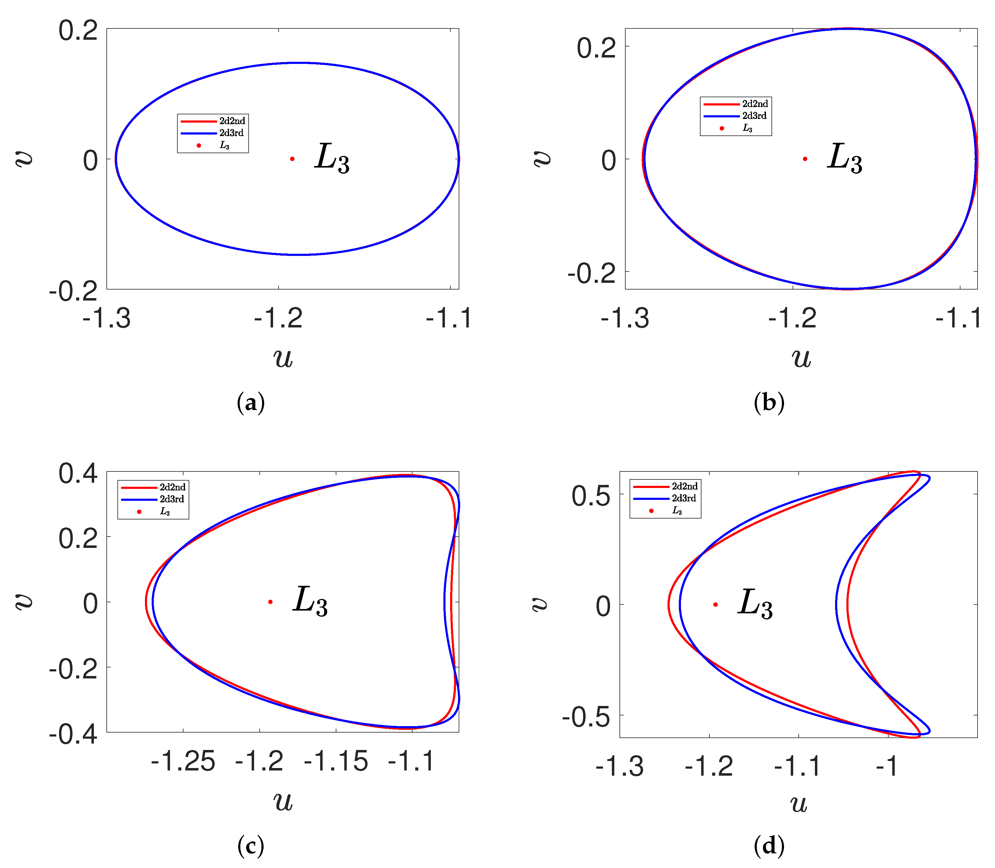
Note that different values of not only determine the positions of the libration points, but also affect the shape of the second- and third-order periodic solutions through Equation (22). This is because the coefficients of Equation (22) are related to (see Appendix A for details). In order to better illustrate the approximate periodic solution obtained above, we show the phase portraits of the above approximate analytical periodic solutions near the libration point under the four cases of , 1, 2, and 4 respectively (see Figure 9a,d). When the value of is small, it is easy to find that the difference between the second- and the third-order approximate periodic solution is insignificant (see Figure 9a,b). Especially for the periodic solutions in Figure 9a, the second- and third-order approximate analytical periodic solutions on the two-dimensional plane around agree very well, and they are almost indistinguishable visually. In this state, the second-order approximate periodic solution can be regarded as the alternative to the third-order case. If the values of other parameters remain unchanged, we can easily find from Figure 9c,d that the difference between the second- and third-order approximate periodic solutions become more and more significant as increases. Therefore, we can conclude according to Figure 9 that the smaller the value of , the better the degree of agreement between the second- and third-order approximate periodic solutions, and vice versa.
5.2. Expansion of Three-Dimensional Dynamic Equations
Applying the translations , and to Equation (7), then we have
Expanding the right hand side of Equation (32) to the second- and to the third-order respectively, then we obtain
and
where the corresponding coefficients are displayed in the Appendix A.
Three-Dimensional Periodic Solutions
By means of successive approximations, we assume that the periodic solution of Equation (33) admits the following form
Substituting Equation (35) into Equation (33) and comparing these terms with the same power e, then we obtain
and
For the third equation of Equation (36), the corresponding periodic solution takes the form
and substitute Equation (38) into the third equation of Equation (36) yields
Note that if there is a non-zero solution to Equation (39), then . So we choose and , and one of the solutions is .
Let the periodic solution of Equation (36) admits the following form
Substituting Equation (40) into Equation (36) and comparing the coefficients of and , then we obtain
and
Similarly, let the periodic solution of Equation (37) has the following form
By using the same method as mentioned above, then we get
Therefore, the periodic solution of Equation (33) with respect to e becomes
where the expressions of these coefficients can be obtained from Appendix B.
As for the third-order approximate periodic solution of Equation (34), suppose that the periodic solution in the form of e can be written as
Substituting Equation (47) into Equation (34), and comparing the terms containing the same power of e, then we obtain three set of equations, the equations corresponding to e and are the same as Equations (36) and (37), respectively, and the equations corresponding to are as follows
Writing the periodic solution of Equations (48) as
Substituting Equations (43), (45) and (49) into Equation (48), and comparing the coefficients of and , then we obtain
Therefore, the third-order approximate analytical periodic solution of Equation (7) in three-dimensional space can be written as
Note that one can find the specific expressions of the above coefficients from Appendix B.
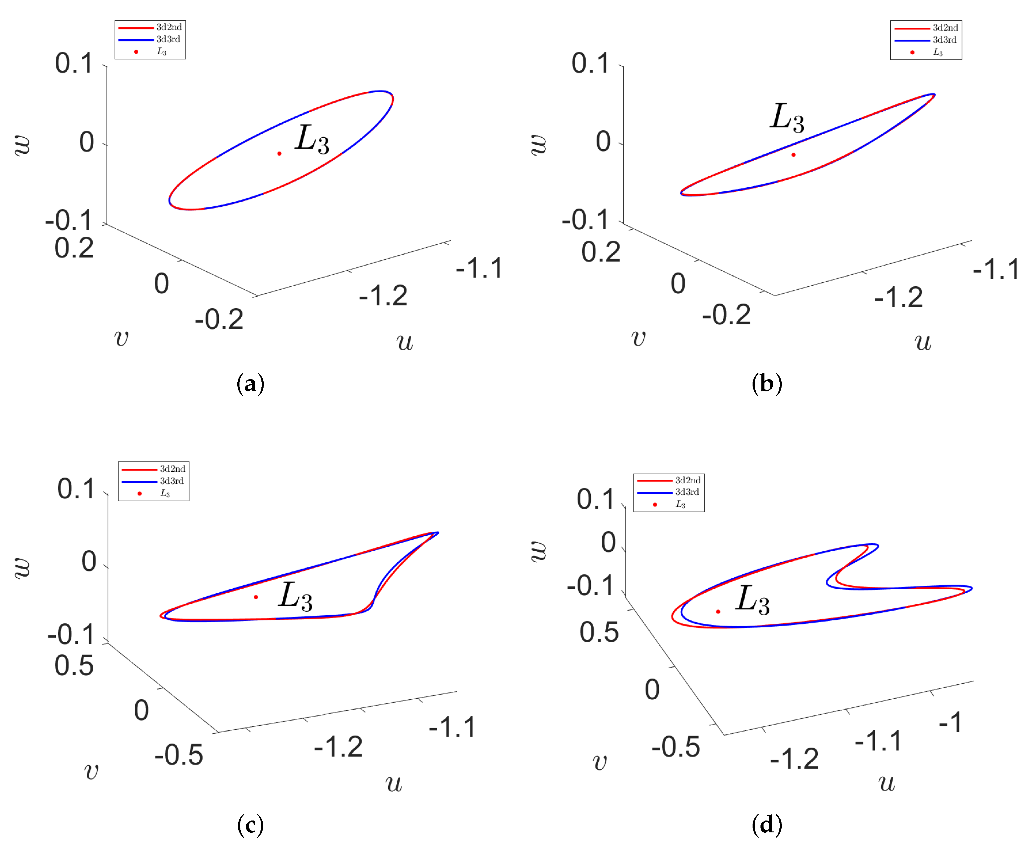
Based on the results of the above analysis, we show the three-dimensional periodic solution near the collinear libration point for four different values of 0.5, 1, 2, and 4 in Figure 10. When and , the second- and third-order three-dimensional periodic solutions agree very well, as shown in Figure 10a,b. When = 2, although Figure 10c shows that the second- and third-order periodic solutions are somewhat different, the degree of agreement is also good. However, Figure 10d (corresponding to = 4) indicates that the second- and third-order periodic solutions differ significantly. Therefore, it is easy to find that the smaller the value of , the better the approximation effect.
6. Conclusions
For a restricted three-body problem consisting of a supergiant eclipsing binary system, we investigated the geometric structure of the corresponding zero-velocity surfaces and curves of the coplanar libration points and discussed the third body’s dynamic behavior under the influence of eight perturbation parameters through bifurcation diagrams. These perturbations include: Coriolis force , centrifugal force , oblateness coefficients and , random sums of the masses of the two primaries, mass ratio parameter , and the primaries’ radiation factors and . We found that any perturbation of Coriolis force and centrifugal force has a greater impact on the third body’s dynamic behavior, but their combined effect has a smaller effect on the third body. Similarly, the oblateness coefficient has a more significant influence on the third body’s dynamic behavior than that of . However, the degree of their combined effect on the third body’s dynamic behavior is minimal. Additionally, the parameter has a more extensive influence on the dynamic behavior of the third body, any tiny changes can cause apparent chaos phenomena. Furthermore, the smaller the mass ratio parameter, the more considerable the dynamic behavior of the third body, and vice versa. Besides, the influence of the radiation factor on the three-body dynamics is more significant than that of . The combined effect of and has a notable effect on the dynamics of the third body when the radiation factor .
In addition, we also applied the Lindstedt-Poincaré perturbation method to present the second- and third-order approximate analytical periodic solutions near the colinear libration points in the plane and space respectively, and illustrated the corresponding phase portraits with respect to , 1, 2, and 4 around the libration point . We found that the smaller the value of , the better the coincidence of the corresponding second-order and third-order periodic solutions. Besides, for the same value, the coincidence between the three-dimensional periodic solutions of different orders is better than that of the two-dimensional case.
Author Contributions
Formal analysis, Y.W.; software, F.G.; writing-original draft, Y.W.; writing—review and editing, F.G. All authors have read and agreed to the published version of the manuscript.
Funding
This research was funded by the National Natural Science Foundation of China (NSFC) though grant No. 11672259, the China Scholarship Council through grant No. 201908320086.
Acknowledgments
We are very grateful to the anonymous reviewers whose comments and suggestions helped improve and clarify this paper.
Conflicts of Interest
The authors declare no conflict of interest.
Appendix A
Appendix B
References
- Marchal, C. The Three-Body Problem; Elsevier Science: New York, NY, USA, 1990. [Google Scholar]
- Ioka, K.; Chiba, T.; Tanaka, T.; Nakamura, T. Black hole binary formation in the expanding universe: Three body problem approximation. Phys. Rev. D 1998, 58, 063003. [Google Scholar] [CrossRef] [Green Version]
- Nakamura, T.; Sasaki, M.; Tanaka, T.; Thorne, K.S. Gravitational waves from coalescing black hole MACHO binaries. Astrophys. J. Lett. 1997, 487, L139. [Google Scholar] [CrossRef] [Green Version]
- Zhou, T.Y.; Cao, W.G.; Xie, Y. Collinear solution to the three-body problem under a scalar-tensor gravity. Phys. Rev. D 2016, 93, 064065. [Google Scholar] [CrossRef]
- Lindner, J.F.; Roseberry, M.I.; Shai, D.E.; Harmon, N.J.; Olaksen, K.D. Precession and chaos in the classical two-body problem in a spherical universe. Int. J. Bifurc. Chaos 2008, 18, 455–464. [Google Scholar] [CrossRef]
- Gao, F.B.; Wang, R.F. Bifurcation analysis and periodic solutions of the HD 191408 system with triaxial and radiative perturbations. Universe 2020, 6, 35. [Google Scholar] [CrossRef] [Green Version]
- Beletsky, V.V. Generalized restricted circular three-body problem as a model for dynamics of binary asteroids. Cosm. Res. 2007, 45, 408–416. [Google Scholar] [CrossRef]
- Hou, X.Y.; Xin, X.S.; Feng, J.L. Forced motions around triangular libration points by solar radiation pressure in a binary asteroid system. Astrodynamics 2020, 4, 17–30. [Google Scholar] [CrossRef]
- Braaten, E.; Kang, D.; Laha, R. Production of dark-matter bound states in the early universe by three-body recombination. J. High Energy Phys. 2018, 2018, 84. [Google Scholar] [CrossRef] [Green Version]
- Trani, A.A.; Fujii, M.S.; Spera, M. The Keplerian three-body encounter. I. Insights on the origin of the S-stars and the G-objects in the galactic center. Astrophys. J. 2019, 875, 42. [Google Scholar] [CrossRef]
- Muzzio, J.C.; Wachlin, F.C.; Carpintero, D.D. Regular and chaotic motion in a restricted three-body problem of astrophysical interest. Int. Astron. Union Colloq. 2000, 174, 281–285. [Google Scholar] [CrossRef] [Green Version]
- Logoteta, D.; Bombaci, I. Constraints on microscopic and phenomenological equations of state of dense matter from GW170817. Universe 2019, 5, 204. [Google Scholar] [CrossRef] [Green Version]
- Fahn, M.J.; Giesel, K.; Kobler, M. Dynamical properties of the Mukhanov-Sasaki Hamiltonian in the context of adiabatic vacua and the Lewis-Riesenfeld invariant. Universe 2019, 5, 170. [Google Scholar] [CrossRef] [Green Version]
- Gao, F.B.; Zhang, W. A study on periodic solutions for the circular restricted three-body problem. Astron. J. 2014, 148, 116. [Google Scholar] [CrossRef] [Green Version]
- Alshaery, A.A.; Abouelmagd, E.I. Analysis of the spatial quantized three-body problem. Results Phys. 2020, 17, 103067. [Google Scholar] [CrossRef]
- Zotos, E.E.; Chen, W.; Abouelmagd, E.I.; Han, H.T. Basins of convergence of equilibrium points in the restricted three-body problem with modified gravitational potential. Chaos Solitons Fractals 2020, 134, 109704. [Google Scholar] [CrossRef]
- Alzahrani, F.; Abouelmagd, E.I.; Guirao, J.L.G.; Hobiny, A. On the libration collinear points in the restricted three-body problem. Open Phys. 2017, 15, 58–67. [Google Scholar] [CrossRef]
- Abouelmagd, E.I.; Guirao, J.L.G.; Llibre, J. Periodic orbits for the perturbed planar circular restricted 3-body problem. Discret. Contin. Dyn. Syst.-Ser. B 2019, 24, 1007–1020. [Google Scholar] [CrossRef] [Green Version]
- Selim, H.H.; Guirao, J.L.G.; Abouelmagd, E.I. Libration points in the restricted three-body problem: Euler angles, existence and stability. Discret. Contin. Dyn. Syst.-Ser. B 2019, 12, 703–710. [Google Scholar] [CrossRef] [Green Version]
- Abouelmagd, E.I.; Mostafa, A.; Guirao, J.L.G. A first order automated lie transform. Int. J. Bifurc. Chaos 2015, 25, 1540026. [Google Scholar] [CrossRef] [Green Version]
- Abouelmagd, E.I.; Asiri, H.M.; Sharaf, M.A. The effect of oblateness in the perturbed restricted three-body problem. Meccanica 2013, 48, 2479–2490. [Google Scholar] [CrossRef]
- Pathak, N.; Thomas, V.O.; Abouelmagd, E.I. The perturbed photogravitational restricted three-body problem: Analysis of resonant periodic orbits. Discret. Contin. Dyn. Syst.-Ser. B 2019, 12, 849–875. [Google Scholar] [CrossRef] [Green Version]
- Niederman, L.; Pousse, A.; Robutel, P. On the co-orbital motion in the three-body problem: Existence of quasi-periodic horseshoe-shaped orbits. Commun. Math. Phys. 2020, 377, 551–612. [Google Scholar] [CrossRef] [Green Version]
- Koon, W.S.; Lo, M.W.; Marsden, J.E.; Ross, S.D. Dynamical Systems, the Three-Body Problem and Space Mission Design; Marsden Books: Wellington, New Zealand, 2011; ISBN 978-0-615-24095-4. [Google Scholar]
- Qian, Y.J.; Yang, X.D.; Yang, L.Y.; Zhang, W. Approximate analytical methodology for the restricted three-body and four-body models based on polynomial series. Int. J. Aerosp. Eng. 2016, 2016, 9747289. [Google Scholar] [CrossRef] [Green Version]
- Pathak, N.; Abouelmagd, E.I.; Thomas, V.O. On higher order resonant periodic orbits in the photo-gravitational planar restricted three-body problem with oblateness. J. Astronaut. Sci. 2019, 66, 475–505. [Google Scholar] [CrossRef]
- Hénon, M. Generating Families in the Restricted Three-Body Problem; Springer: New York, NY, USA, 1997. [Google Scholar]
- Chenciner, A.; Montgomery, R. A remarkable periodic solution of the three-body problem in the case of equal masses. Ann. Math. 2000, 152, 881–901. [Google Scholar] [CrossRef] [Green Version]
- Šuvakov, M.; Dmitrašinović, V. Three classes of Newtonian three-body planar periodic solutions. Phys. Rev. Lett. 2013, 110, 114301. [Google Scholar] [CrossRef] [Green Version]
- Janković, M.R.; Dmitrašinović, V.; Šuvakov, M. A guide to hunting periodic three-body orbits with non-vanishing angular momentum. Comput. Phys. Commun. 2020, 250, 107052. [Google Scholar] [CrossRef]
- Li, X.M.; Liao, S.J. More than six hundred new families of Newtonian periodic planar collisionless three-body orbits. Sci. China Phys. Mech. Astron. 2017, 60, 129511. [Google Scholar] [CrossRef] [Green Version]
- Kalantonis, V.S. Numerical investigation for periodic solutions in the Hill three-body problem. Universe 2020, 6, 72. [Google Scholar] [CrossRef]
- Singh, J. Photogravitational restricted three-body problem with variable mass. Indian Indian J. Pure Appl. Math. 2003, 34, 335–341. [Google Scholar]
- Singh, J.; Leke, O. Stability of the photogravitational restricted three-body problem with variable masses. Astrophys. Space Sci. 2010, 326, 305–314. [Google Scholar] [CrossRef]
- Singh, J.; Leke, O. Equilibrium points and stability in the restricted three-body problem with oblateness and variable masses. Astrophys. Space Sci. 2012, 340, 27–41. [Google Scholar] [CrossRef]
- Singh, J.; Leke, O. Effect of oblateness, perturbations, radiation and varying masses on the stability of equilibrium points in the restricted three-body problem. Astrophys. Space Sci. 2013, 344, 51–61. [Google Scholar] [CrossRef]
- Singh, J.; Haruna, S. Equilibrium points and stability under effect of radiation and perturbing forces in the restricted problem of three oblate bodies. Astrophys. Space Sci. 2014, 349, 107–116. [Google Scholar] [CrossRef]
- Singh, J.; Perdiou, A.E.; Gyegwe, J.M.; Kalantonis, V.S. Periodic orbits around the collinear equilibrium points for binary Sirius, Procyon, Luhman 16, α-Centuari and Luyten 726-8 systems: The spatial case. J. Phys. Commun. 2017, 1, 025008. [Google Scholar] [CrossRef]
- Singh, J.; Perdiou, A.E.; Gyegwe, J.M.; Perdios, E.A. Periodic solutions around the collinear equilibrium points in the perturbed restricted three-body problem with triaxial and radiating primaries for binary HD 191408, Kruger 60 and HD 155876 systems. Appl. Math. Comput. 2018, 325, 358–374. [Google Scholar] [CrossRef]
- Abdulraheem, A.R.; Singh, J. Combined effects of perturbations, radiation and oblateness on the periodic solutions in the restricted three-body problem. Astrophys. Space Sci. 2008, 317, 9–13. [Google Scholar] [CrossRef] [Green Version]
- Abdulraheem, A.R.; Singh, J. Combined effects of perturbations, radiation, and oblateness on the stability of equilibrium points in the restricted three-body problem. Astron. J. 2006, 131, 1880. [Google Scholar] [CrossRef]
- Singh, J.; Ishwar, B. Effect of perturbations on the location of equilibrium points in the restricted problem of three bodies with variable mass. Celestial Mech. 1984, 32, 297–305. [Google Scholar] [CrossRef]
- Bhatnagar, K.B.; Chawla, J.M. A study of the Lagrangian points in the photogravitational restricted three-body problem. Indian J. Pure Appl. Math. 1979, 10, 1443–1451. [Google Scholar]
- Szebehely, V. Stability of the points of equilibrium in the restricted problem. Astron. J. 1967, 72, 7–9. [Google Scholar] [CrossRef]
- Subba Rao, P.V.; Sharma, R.K. Perturbations of the critical mass in the restricted three-body problem. Astrophys. Space Sci. 1976, 42, L17–L18. [Google Scholar]
- Sharma, R.K. Perturbations of Lagrangian points in the restricted three-body problem. Indian J. Pure Appl. Math. 1975, 6, 1099–1102. [Google Scholar]
- Sharma, R.K.; Subba Rao, P.V. Stationary solutions and their characteristic exponents in the restricted three-body problem when the more massive primary is an oblate spheroid. Celestial Mech. 1976, 13, 137–149. [Google Scholar] [CrossRef]
- Abdullah, A.A.; Alhussain, Z.A.; Kellil, R. Locations and stability of the libration points in the CR3BP with perturbations. J. Math. Anal. 2017, 8, 131–144. [Google Scholar]
- Abouelmagd, E.I.; Alzahrani, F.; Hobiny, A.; Guirao, J.L.G.; Alhothuali, M. Periodic solutions around the collinear libration points. J. Nonlinear Sci. Appl. 2016, 9, 1716–1727. [Google Scholar] [CrossRef]
- Bekov, A.A. Particular solutions in the restricted collinear three body problem with variable masses. Soviet Astron. 1991, 35, 103–106. [Google Scholar]
- Zotos, E.E. How does the oblateness coefficient influence the nature of solutions in the restricted three-body problem? Astrophys. Space Sci. 2015, 358, 33. [Google Scholar] [CrossRef] [Green Version]
- Bhatnagar, K.B.; Hallan, P.P. Effect of perturbations in Coriolis and centrifugal forces on the stability of libration points in the restricted problem. Celestial Mech. 1978, 18, 105–112. [Google Scholar] [CrossRef]
- Subbarao, P.V.; Sharma, R.K. A note on the stability of the triangular points of equilibrium in the restricted three-body problem. Astron. Astrophys. 1975, 43, 381–383. [Google Scholar]
- Gyldén, H. Die bahnbewegungen in einem systeme von zwei Körpern in dem falle, dass die massen veränderungen unterworfen sind. Astron. Nachr. 1884, 109, 1–6. [Google Scholar] [CrossRef] [Green Version]
- Bekov, A.A. Periodic solutions of the Gylden-Meshcherskii problem. Astron. Rep. 1993, 37, 651–654. [Google Scholar]
- Bekov, A.A.; Momynov, S.B. Parametric solutions of the Gylden-Meshchersky problem. Int. J. Non-Linear Mech. 2019, 116, 195–199. [Google Scholar] [CrossRef]
- Meshcherskii, I.V. Works on the Mechanics of Bodies of Variable Mass; GITTL: Moscow, Russia, 1952; p. 205. (In Russian) [Google Scholar]
- Kalantonis, V.S.; Perdios, E.A.; Perdiou, A.E.; Vrahatis, M.N. Computing with certainty individual members of families of periodic orbits of a given period. Celestial Mech. Dyn. Astron. 2001, 80, 81–96. [Google Scholar] [CrossRef]
- Hu, H.Y. Applied Nonlinear Dynamics; China Aeronautical Industry Press: Beijing, China, 2000. (In Chinese) [Google Scholar]
Figure 1.
Zero velocity surfaces for and 4, respectively.

Figure 2.
Zero-velocity surfaces of the third body for : (a) , (b) , (c) , (d) .

Figure 3.
Zero-velocity curves of the third body: (a) , (b) , (c) , (d) .

Figure 4.
(a–c) Bifurcation diagrams of Coriolis force and centrifugal force in the frames , and , respectively, when .
Figure 4.
(a–c) Bifurcation diagrams of Coriolis force and centrifugal force in the frames , and , respectively, when .

Figure 5.
(a–c) Bifurcation diagrams of oblateness coefficient of the ith () primary in the frames , and , respectively, when , , , , , .
Figure 5.
(a–c) Bifurcation diagrams of oblateness coefficient of the ith () primary in the frames , and , respectively, when , , , , , .

Figure 6.
(a–c) Bifurcation diagrams of the arbitrary sum of the masses of the primaries in the frames , and , respectively, when .
Figure 6.
(a–c) Bifurcation diagrams of the arbitrary sum of the masses of the primaries in the frames , and , respectively, when .

Figure 7.
(a–c) Bifurcation diagrams of the mass parameter in the frames , and , respectively, when , .
Figure 7.
(a–c) Bifurcation diagrams of the mass parameter in the frames , and , respectively, when , .

Figure 8.
(a–c) Bifurcation diagrams of radiation factor of the ith () primary in the frames , and , respectively, when .
Figure 8.
(a–c) Bifurcation diagrams of radiation factor of the ith () primary in the frames , and , respectively, when .

Figure 9.
The approximate periodic solutions in two-dimensional plane for (a) , (b) , (c) , and (d) , respectively.
Figure 9.
The approximate periodic solutions in two-dimensional plane for (a) , (b) , (c) , and (d) , respectively.

Figure 10.
The approximate periodic solutions in three-dimensional space for (a) , (b) , (c) , and (d) , respectively.
Figure 10.
The approximate periodic solutions in three-dimensional space for (a) , (b) , (c) , and (d) , respectively.


Table 1.
Physical parameters in Equation (7).
Table 1.
Physical parameters in Equation (7).
| Parameters | |||||||
| Values | 0.48785 | 0.9988 | 0.9985 | 0.024 | 0.02 | 1.001 | 1.002 |
© 2020 by the authors. Licensee MDPI, Basel, Switzerland. This article is an open access article distributed under the terms and conditions of the Creative Commons Attribution (CC BY) license (http://creativecommons.org/licenses/by/4.0/).
Share and Cite
MDPI and ACS Style
Gao, F.; Wang, Y. Approximate Analytical Periodic Solutions to the Restricted Three-Body Problem with Perturbation, Oblateness, Radiation and Varying Mass. Universe 2020, 6, 110. https://doi.org/10.3390/universe6080110
AMA Style
Gao F, Wang Y. Approximate Analytical Periodic Solutions to the Restricted Three-Body Problem with Perturbation, Oblateness, Radiation and Varying Mass. Universe. 2020; 6(8):110. https://doi.org/10.3390/universe6080110
Chicago/Turabian StyleGao, Fabao, and Yongqing Wang. 2020. "Approximate Analytical Periodic Solutions to the Restricted Three-Body Problem with Perturbation, Oblateness, Radiation and Varying Mass" Universe 6, no. 8: 110. https://doi.org/10.3390/universe6080110
Note that from the first issue of 2016, this journal uses article numbers instead of page numbers. See further details here.