Article

Predicting Land Cover Change in the Mamminasata Area, Indonesia, to Evaluate the Spatial Plan

by
Andi Muhammad Yasser Hakim
1,2,*,
Masayuki Matsuoka
2,
Sumbangan Baja
1,
Dorothea Agnes Rampisela
1,3 and
Samsu Arif
4,5
1
Department of Soil Science, Faculty of Agriculture, Hasanuddin University, Makassar 90245, Indonesia
2
Faculty of Agriculture and Marine Science, Kochi University, Kochi 783-8502, Japan
3
Research Institute for Humanity and Nature, Kyoto 603-8047, Japan
4
Department of Physics, Faculty of Mathematics and Natural Science, Hasanuddin University, Makassar 90245, Indonesia
5
Centre for Regional Development and Spatial Information (WITaRIS), Hasanuddin University, Makassar 90245, Indonesia
*
Author to whom correspondence should be addressed.
ISPRS Int. J. Geo-Inf. 2020, 9(8), 481; https://doi.org/10.3390/ijgi9080481
Submission received: 6 July 2020 / Revised: 29 July 2020 / Accepted: 3 August 2020 / Published: 4 August 2020

Abstract

:
The spatial plan program for Makassar City and the surrounding area called Mamminasata (Makassar, Maros, Sungguminasa, and Takalar) was created by the Indonesian Government. The program regulates the proportion of land cover, but predictions about land cover changes were not considered. Therefore, in this study, we predict what the land cover may be in 2031 using the multi-layer perceptron neural network and the Markov chain methods. For this purpose, image composite, support vector machine classifier, and change detection were applied to a time series of satellite data. Visual validation showed the hot-spots of land cover changes related to population density, and statistical validation scored 0.99 and 0.78 in no information kappa and grid-cell level location kappa, respectively. The model was performed to predict land cover in 2031, and the predicted result was then compared with the spatial plan using an overlapping method. The results showed that built-up area, dryland agriculture, and wetland agriculture occupied two, twenty, and eight percent of the protected zone, respectively. Meanwhile, fifteen percent of the development zone was covered by forest, mainly in the eastern part of Mamminasata. The result can be used to help the Government decide future plans for the Mamminasata area.

1. Introduction

The concept of sustainable development was established at Agenda 21 in Rio de Janeiro [1], leading to many countries, especially developing countries, striving to achieve the goals of the concept. The core concept comprised of three pillars, namely, social, economic, and environmental [2]. Many issues that affect sustainable development are geospatially interrelated and can be analyzed, modeled, and mapped within a geographic context [3]. Indonesia, as a developing country and a newly industrialized country that flourished in the mid-1990s [4], has applied the concept of sustainable development in spatial plan programs. These programs contain regulations related to the proportion of land cover area in a region. In the Mamminasata area, South Sulawesi province, the local government has established the spatial plan since 2006. Several issues related to the condition of land cover and spatial plan in this area had been addressed [5], such as: (a) the existing spatial plan was paying less attention to its implementation, especially for the conservation, protection and hazardous areas; (b) balance between the current land cover and future development were not fully taken into account under the existing spatial plan; and (c) lack of coordination among government agencies and institutions. Another important issue was that the land cover prediction has not been considered in the spatial plan.
Several researchers have studied the relationship between sustainable development and land cover change. García-Ruiz et al. [6] linked the effects of land use change on sustainable development in the Pyrenees mountain areas, Spain. Musa et al. [7] modeled the development of cities based on land cover changes for sustainable development in the Niger Delta Region, Nigeria. Salazar et al. [8] combined urban planning, natural conservation, and risk areas to build a prediction model for land use change as a guide for sustainable development in the Quito Metropolitan District, Ecuador. Land cover change is an important part of achieving sustainable development.
To simulate and predict land cover changes, a variety of models have been applied, mainly by combining remote sensing (RS) and a geographic information system (GIS) [9,10]. Losiri et al. [11] classified those models into four types: (a) empirical and statistical models such as the Markov chain and logistic regression; (b) dynamic models such as cellular automata, agent-based model, genetic algorithm, artificial neural network, and system dynamic; (c) integrated models such as conversion of land use and its effects at small regional extent (CLUE-S) and Dyna-CLUE; and (d) hybrid models such as Metronamica, land transformation model, land change modeler (LCM), and slope, land use, exclusion, urban extent, transportation, and hill-shade (SLEUTH).
The multi-layer perceptron neural network and the Markov chain (MLPNN + MC) in LCM was found to produce a considerably higher prediction accuracy than other models [11,12,13,14,15]. This higher prediction accuracy stems from neural networks being able to express changes in various land cover types more adequately than single probabilities such as the weights of evidence method [13]. The three layers (input, hidden, output) in MLPNN are used to express complex non-linear relationships between land cover changes and driving factors that produce transition potential, while the transition potential matrix is calculated by using MC to predict future land cover changes [10]. Based on the work of Pickard et al. [16], LCM has four specific characteristics and advantages: (a) flexible input data in pre-processing and the data collection process; (b) probability surface, exclusion layer, and regional stratification in the calibration process; (c) stochastic modeling to generate the model projections process; and (d) dynamic variables allowed and scenario analysis in extrapolating future scenarios. This model has been used in several studies on urban growth simulation [14,17,18], spatial dynamics of deforestation and fragmentation [19], land use changes following green infrastructure policies [20], and so on.
To obtain land cover classification, the support vector machine (SVM) with its non-linearity and multidimensional capabilities is a good choice because this method has a powerful image classification technique for handling multispectral satellite imagery [21]. For two or more periods, change detection can be applied to monitor land cover dynamics. Change detection methods are grouped into two categories: unsupervised direct comparison (UDC) and supervised post-classification comparison (SPCC) [22]. UDC is relatively simple and straightforward, and does not require a manually labeled training set [23], whereas SPCC uses an image object as the basic unit in change analysis and simultaneously detects the area and type of change [24]. Another simple change detection method is change vector analysis (CVA), which computes spectral change vectors using given multi-dates and compares their magnitudes with a specified threshold criterion [25]. Land cover classification is an important part of predicting land cover change, and is a common research tool that is often used for determining actual [26], previous [27,28,29,30], and future [9,31,32] land cover. Land cover classification and change detection are also supported by availability and access, as well as its continuity and affordability of medium- to low-resolution remote sensing data that can be provided free of charge [33].
The purpose of this research was to predict land cover in 2031 in the Mamminasata area, Indonesia, by using the multi-layer perceptron neural network and the Markov chain. The support vector machine and change vector analysis were used to obtain land cover classification in 2006, 2011, and 2016. Seven vector maps made by the Government were used as driving factors. The prediction model was validated using visual and statistical methods. The predicted land cover in 2031 was compared and evaluated with the Government’s spatial plan for the period from 2011 to 2031 using the overlapping method.

2. Research Site and Materials
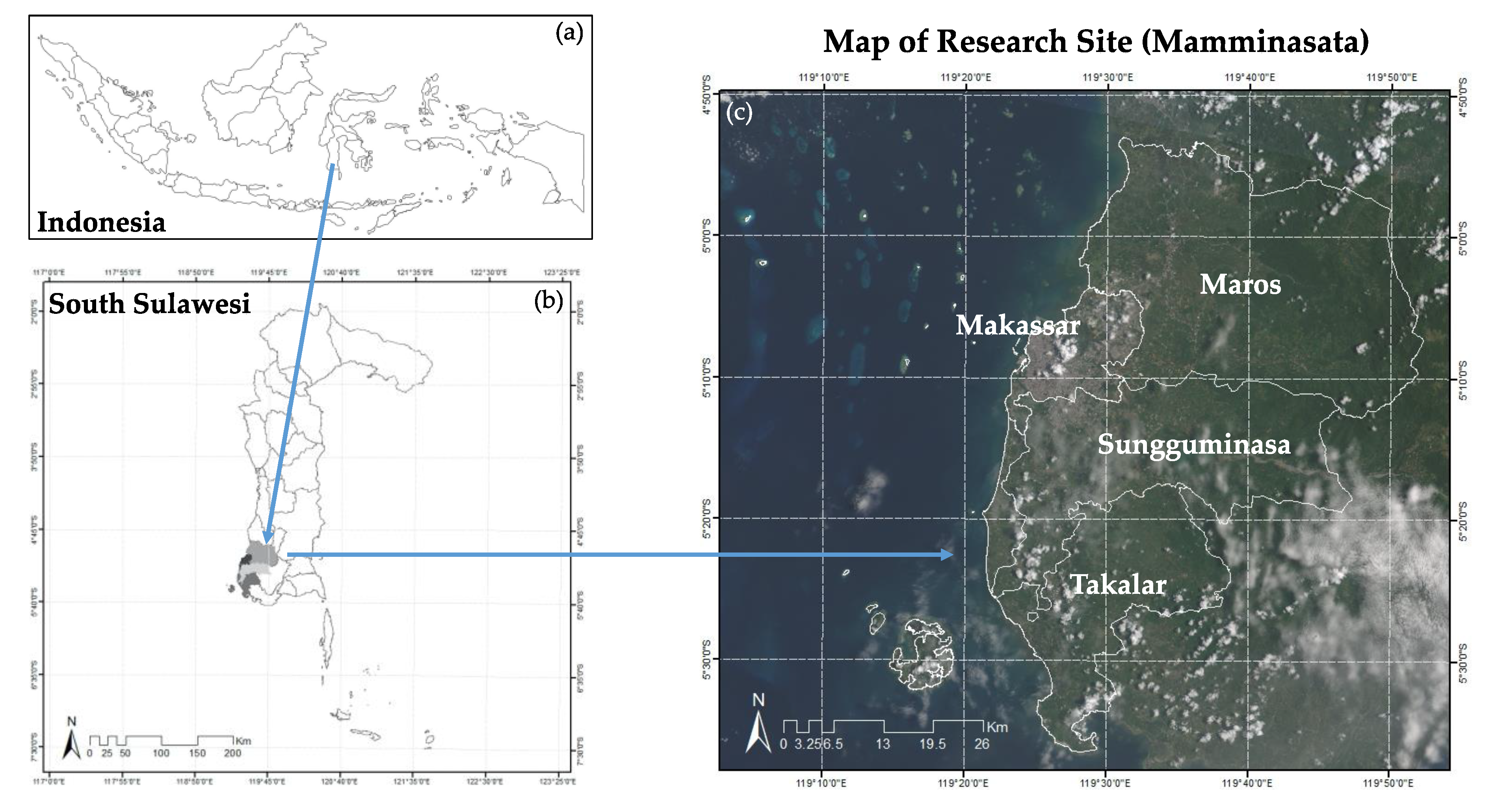
2.1. Research Site

The Mamminasata Urban Area in Sulawesi Island, Indonesia, has an area of 247,000 ha and consists of Makassar, Maros, Sungguminasa, and Takalar municipalities (Figure 1). The area was established by a decree of the Governor of South Sulawesi province in 2003 because of the development of Makassar City, the capital of the South Sulawesi province. Makassar City has grown rapidly, resulting in agglomeration with the other three municipalities. In addition, the Mamminasata area is the economic center area in Eastern Indonesia and contributes a significant proportion of the gross regional domestic product of the South Sulawesi province: 39% in 2006, 44% in 2011, and 45% in 2016 [34,35,36].
The Government has created a spatial plan for 2011–2031 to make the Mamminasata Urban Area the center of international-scale services in Eastern Indonesia with the aim of achieving sustainable development. To bolster the plan, the Indonesian Government established the Mamminasata Urban Area as a national strategic area, with the aims of having this area act as a model metropolitan area and as an exemplar of urban development for Indonesia [37].

2.2. Materials

2.2.1. Satellite Data

Landsat 7 Enhanced Thematic Mapper plus (ETM+) and Landsat 8 Operational Land Imager (OLI) were used in this study because of the availability of long-term data free of charge. The observation dates are listed in Table 1. Two consecutives scenes, 116/63 and 116/64 for path/row, were downloaded from the United States Geological Survey (USGS) [38]. Six bands from 1 to 7 except band 6 were used from Landsat 7 ETM+, and corresponding bands from 2 to 7 were used from Landsat 8 OLI. Map projection was in the Universal Transverse Mercator (UTM) Zone 50 South, and spatial resolution was 30 meters. Data were converted into top of the atmosphere reflectance in 8 bits. We selected less cloudy scenes from two seasons in Indonesia (wet season from November to May and dry season from June to September). In addition, multiple scenes were used for each season to avoid the remaining cloud and its shadows, and to fill the scan gaps in Landsat 7 ETM+.

2.2.2. Other Spatial Data

Vector data of capital, river and lake, road and settlement were used as driving factors; land use as the training data; and administration area as a boundary map of Mamminasata. In addition, elevation and slope were used based on a 30-meter resolution digital elevation model (DEM) generated by the Shuttle Radar Topography Mission (SRTM). The population density of the Mamminasata area in 2011 was used to calculate a population density per pixel as a driving factor. All data were converted into raster format at a resolution of 30 meters to apply LCM. These data were obtained from the database of the Centre for Regional Development and Spatial Information (WITaRIS), Hasanuddin University [37].

3. Methods

The integrated method used in this research required three mains steps. In Step 1, a land cover map for 2011 was derived using composite method and SVM classifier, and land cover maps for 2006 and 2016 were derived by change detection. In Step 2, land cover change was modeled by MLPNN + MC using three land cover maps, several driving factors, and a parameter set. MLPNN was carried out to obtain transition potential between 2006 and 2011, while MC was applied to predict land cover in 2016 and 2031. In Step 3, predicted land cover in 2031 was overlaid with the Government’s spatial plan. The result was used to evaluate the spatial plan and to help guide the future development of Mamminasata.

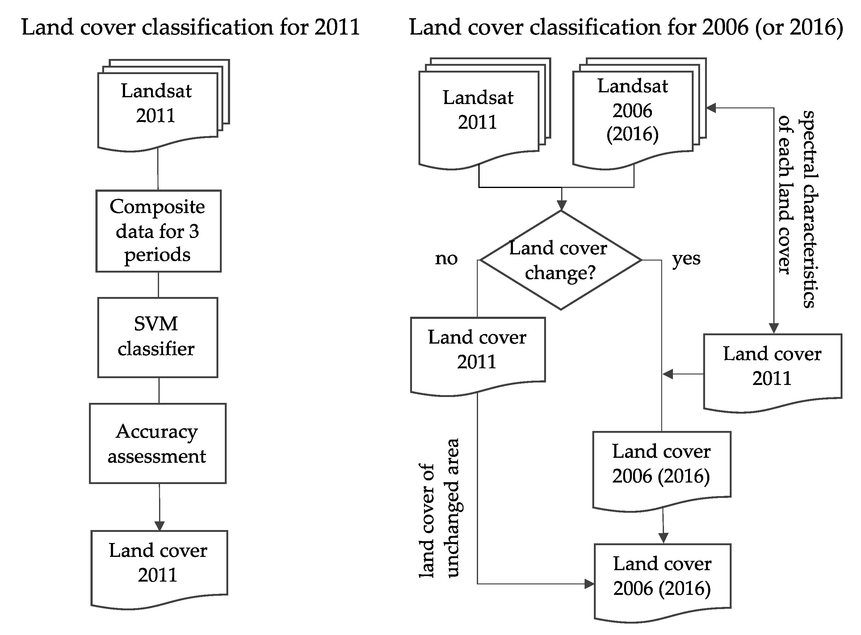
3.1. Land Cover Mapping

We used two schemes to obtain the land cover classification maps (Figure 2). First, we generated a land cover map for 2011 through image classification (left side). Second, land cover maps for 2006 and 2016 were generated through change detection with 2011 (right side). The right side of Figure 2 shows the case for 2011 and 2006, but the flow is the same for 2011 and 2016.

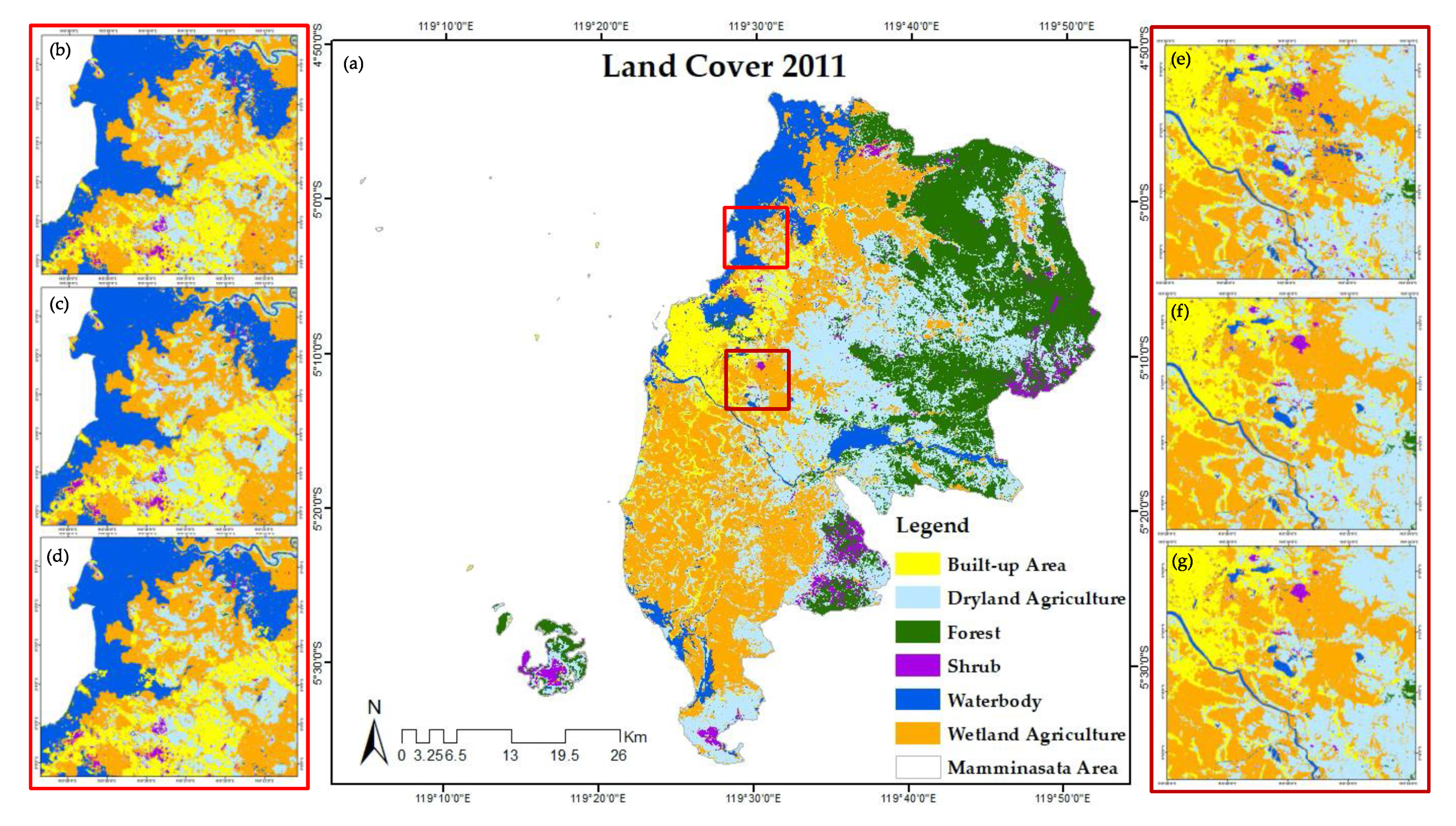
3.1.1. Land Cover in 2011

Areas covered by cloud and shadow are obstacles in optical remote sensing. The cloud masking method is an important solution to this problem [39]. We used cloud mask included in Landsat data to detect cloud and its shadow. In addition, image processing is often necessary prior to land cover classification, especially with the presence of striping scan gaps as occurred in the Landsat-7 ETM+ images [40] because of the failure of the Scan Line Corrector (SLC) since May 2003, which causes systematic data gaps on the captured imagery and eliminated the capacity to provide spatially continuous fields [41].
To fill-in the cloud and shadow areas and scan gaps in the Landsat ETM+ data, a two-step composite was applied prior to the land cover classification as follows. In the first step, two cloudless scenes were selected from images observed in the same season to minimize seasonal change (Table 2). A pixel-based composite was created using these images and based on the following rules: (1) no data were selected if both pixels were cloud, shadow, or scan gap; (2) if one of the two images was clear data, it was selected; and (3) if both data were fine, the difference between the near infrared band (Band 4) and red band (Band 3) was calculated, and the pixel with the larger difference was selected. The last rule was adopted to avoid a thin cloud and its shadow, and the smoothness of the image could be kept by selecting neighboring pixels from the same image.
Although most of the pixels were filled-in during the first step, blank pixels remained if both image pixels were cloud, shadow, or scan gap. Blank pixels are unfavorable for land cover classification, so the second step was applied only to those blank pixels. Candidate images were selected from a similar season, although these images were from longer range of observation dates compared with the first step because fewer cloud-free scenes were available for our site. If the first composite image was a blank pixel, it was filled-in using the following procedure: (1) the 5 × 5 pixel block with the blank pixel at the center was selected from the composite image; (2) the sum of absolute difference between the composite image and each candidate image for all bands was calculated by using clear data; and (3) the pixel with the minimum difference was selected from the image.
The two-step procedure was adopted because a blank pixel has small patches, and a smooth image was generated by using a pixel block for the comparison. We started with a small number of candidate images and increased the number of images by checking the composite result. Using this composite method, three scenes were generated for different seasons to achieve high classification accuracy. We could not generate better images for other seasons because of heavy cloud cover and fewer available images.
A support vector machine (SVM) was adopted as a land cover classifier because it has been evaluated as a high-performance machine-learning algorithm and has been investigated in a number of studies [26,30,42,43]. In this study, the pixel-based classification was applied using six bands of three composite scenes. The pixel-based technique is generally used for land cover classifications with medium-resolution imagery at the regional level [44]. In addition, SVM is better at recognizing subtle patterns in complex datasets compared with other machine-learning methods [45]. This classifier is a kernel-based supervised-learning algorithm, which combines machine-learning theory, optimization algorithms from operations research, and kernel techniques from mathematical analysis [46].
The training area was extracted from the land use map that was produced by the Government in 2011 [37]. The original map contains 29 land use types, which we merged into six land cover types (built-up area, dryland agriculture, forest, shrub, waterbody, and wetland agriculture) for our purpose to apply the land cover map for spatial prediction modeling. The 30-meter-wide boundary of land use polygons in the training map was excluded to eliminate mixture of land cover in the training samples. Spectral reflectances of Landsat data (6 bands x 3 scenes) were extracted with respect to each land cover by overlapping the training map and Landsat images. These processes were carried out using ArcGIS software (ESRI, Redlands, CA, USA). The reflectances of all land cover types were subsequently input to the Statistic and Machine Learning Toolbox of MATLAB software (MathWorks, Natick, MA, USA). All the available samples were used as training data for the SVM classifier.
Because almost the whole area except the boundary was covered by the training data, the classification map was similar to the Government map. Therefore, accuracy was assessed only in areas that had different land cover types between the training data and the SVM classification. We picked 100 check points for each land cover class from a Google Earth image. A confusion matrix was generated and producer’s accuracy (PA), user’s accuracy (UA), overall accuracy (OA), agreement of chance (AoC), and kappa coefficient (KC) were calculated using the following formulas [47]:
P A = C a C g · s u m
U A = C a C i · s u m
O A = C c · s u m C · s u m
A o C = P M ( C · s u m ) 2
K C = O A A o C 1 A o C
where
Ca:number of points where classification is correct,
Cg·sum:total ground truth points per class,
Ci·sum:total classification points per class,
Cc·sum:total number of points where classification is correct,
C·sum:total number of points,
PM:sum of the multiplication of ground truth points and classification points with respect to each land cover.

3.1.2. Land Cover in 2006 and 2016

Land cover classification maps in 2006 and 2016 were obtained through change detection with 2011, and land cover was identified only in the pixels where change was detected. Asokan and Anitha [48] classified the change detection approach into five types: algebra based, transform based, classification based, GIS, and an advanced model. Hussain et al. [44] summarized the differences between several change detection techniques into three types: pixel based, object based, and spatial data mining. Based on these studies, we used a pixel-based technique through an algebra-based approach (image differencing). This technique is based on the direct comparison between two images; the advantages are simple and easy to interpret [44]. In addition, this technique is suitable for use in medium-resolution imagery such as that from Landsat [44]. A common procedure in algebra-based change detection is the threshold selection to find the changed area [48].
In this change detection, the same method was applied to two periods (2011–2006 and 2011–2016) individually using four pairs of images listed in Table 3. The degree of change was calculated using the following equation:
D n ( i , j ) = 1 P × 6 p = 1 P b = 1 6 ( D p , b ( i , j ) D p , b ¯ σ D p , b ) 2
where
D n ( i , j ) :normalized difference for the image pixel at location i (line) and j (column),
P :number of valid image pair (maximum is 4 but it is decreased in case of cloud, shadow, and scan gap),
D p , b ( i , j ) :difference in digital number between 2011 and 2006 (or 2016) at pixel ( i , j ) ( b and p are index for band and image pair, respectively),
D p , b ¯ :average of D p , b ( i , j ) for all pixels in a scene,
σ D p , b :standard deviation of D p , b ( i , j ) for all pixels in a scene.
For Band (b), we used six bands from 1 to 7 except band 6 from Landsat 7, and Bands from 2 to 7 from Landsat 8. This equation means that the same weight was given for all bands because the variation in difference by band was normalized using average and standard deviation of the pixel difference by each band. It should be noted that the difference could be calculated if both image pixels have valid data. If one of the pair is cloud, shadow, or scan gap, the pixel is excluded from the calculation of Dn(i,j). In order to minimize the difference of TM and ETM+ spectral responses, the normalized difference was calculated using top of the atmosphere reflectance, not the digital number of the image. In addition, the residual difference could be eliminated by subtracting the average of difference ( D p , b ¯ ) in normalization process. After calculating this normalized difference, the land cover change was detected by applying the threshold, which was selected manually by comparing the detected area with a time series of Google Earth fine-resolution satellite images.
The new land cover was identified for the changed area based on the following method: (1) sample data (20,000 pixels) were selected from unchanged areas in 2006 (or 2016) images for all six land cover types; (2) for each changed pixel, the differences with the above sample data were calculated using Equation (7); (3) these differences were sorted in ascending order; and (4) by evaluating the first 20,000 samples, land cover was identified by the most common land cover among the six types.
D ( c , s ) = 1 P × 6 p = 1 P b = 1 6 ( R p , b R c , s , p , b σ R c , p , b ) 2
where
D ( c , s ) :normalized difference for the image pixel at location i (line) and j (column),
P :number of valid image pair (maximum is 4 but it is decreased in case of cloud, shadow, and scan gap),
R p , b :digital number of changed pixel ( b and p are index for band and image pair, respectively),
R c , s , p , b :digital number of sample data as same band and period with R p , b for sample data s in land cover class c ,
σ R c , p , b :standard deviation of R c , s , p , b for all samples.
This method assigns the changed pixel to the nearest class based on the spectral reflectance of each land cover sample extracted from an unchanged area. Therefore, the method allows change between the same classes, e.g., from dryland agriculture to dryland agriculture, even if the pixel was regarded as a changed pixel. We adopted this “change detection and classification” scheme in order to cope with the variations of spectral reflectance due to sensor and season. These biases were compensated by comparing the reflectance of changed pixel with samples extracted from same scene. Change detection and subsequent determination of land cover type were carried out using self-coded software.

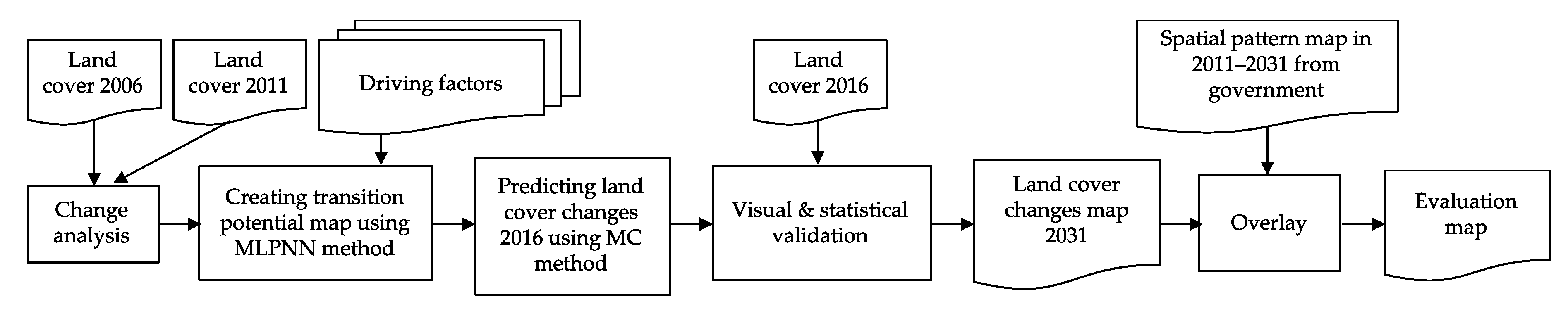
3.2. Land Cover Change Model

The land change modeler (LCM) module embedded in TerrSet software (Clark Labs, Worcester, MA, USA) was used in this study. The module developed by Clark Labs analyzes land cover changes, evaluates driving factors, calculates transition potential from one class to another, and builds a model prediction of land cover changes empirically, which can be tested for accuracy [10,18,49,50]. This module has been recognized as an effective tool in predicting land use change, with an easy-to-understand user interface [10].
To model land cover change, LCM requires three maps: maps from two previous periods are used to optimize the prediction model for the third period by comparing with the map of the third period [51]. We used the 2006 and 2011 maps to build the model by referring to the 2016 map. Figure 3 shows a land cover change modeling flowchart. Land cover maps in 2006 and 2011 were used to predict land cover in 2016 by applying the MLPNN method coupled with driving factors. Predicted land cover for 2016 was generated by applying the MC method, and the prediction result was validated visually and statistically. If the accuracy value is acceptable, the model can be applied to the prediction for 2031. Consequently, land cover prediction for 2031 was overlaid with the Government’s spatial plan map for 2011–2031. The result was used as an evaluation map for future development of the Mamminasata area.

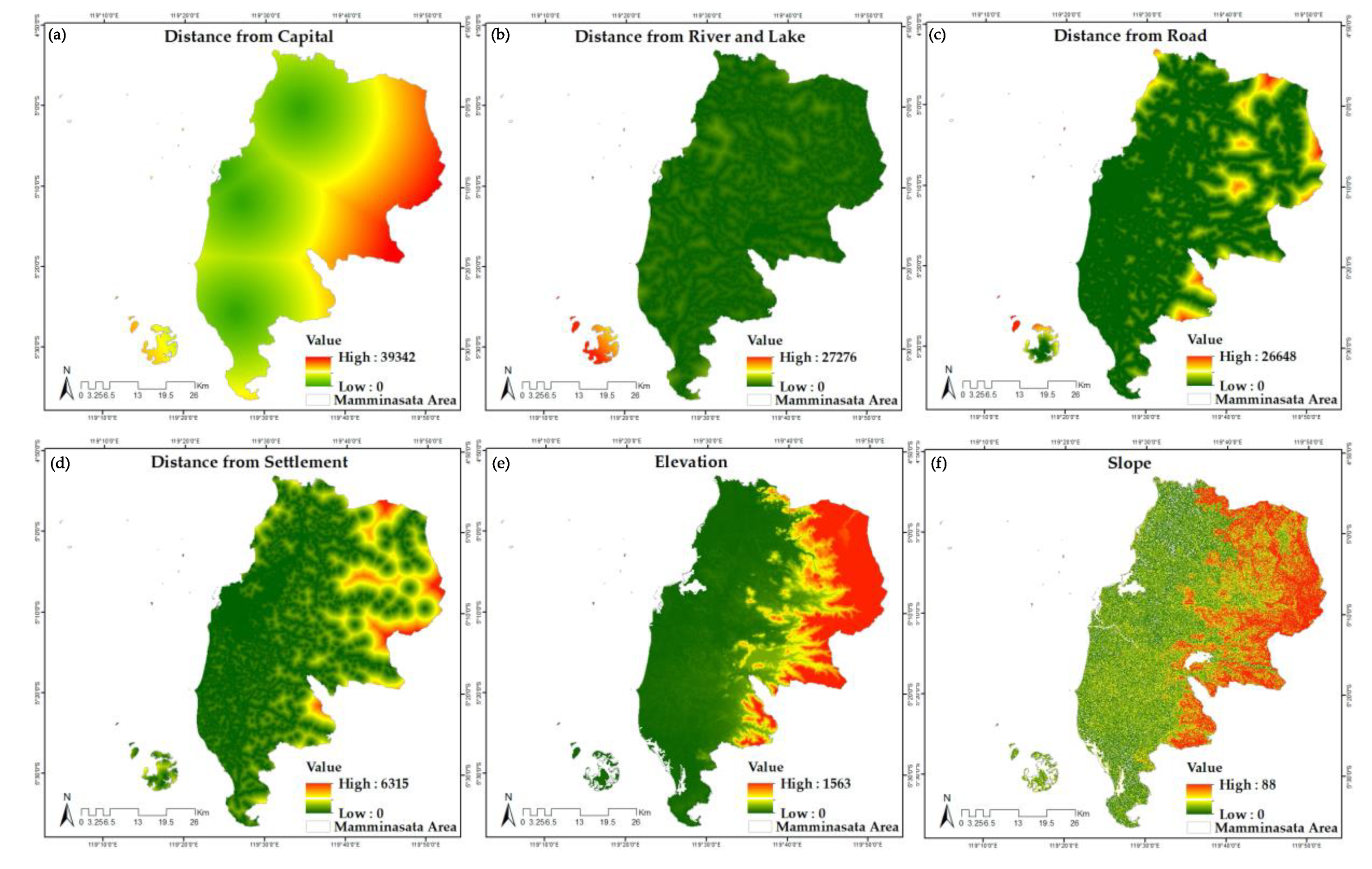
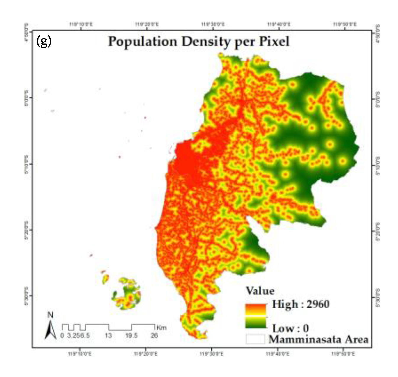
3.2.1. Driving Factors

A driving factor is a variable that forces a change in land cover. Seven driving-factor maps (distance from capital, distance from river and lake, distance from road, distance from settlement, elevation, slope, and population density per pixel) were used to model land cover prediction. These driving factors were selected due to the availability of these data. The slope was calculated in the Slope module using DEM. The four distance maps were processed in the Distance module using vector maps of capital, river and lake, road and settlement, respectively. The population density per pixel was obtained using the following formula:
K p = p × A × P × C
where
Kp:
population density per pixel,
p:
population density of Mamminasata (= 981.29 people/km2 [52]),
A:
population distribution area (= 3.14 × (2 km)2 = 12.56 km2),
P:
population proportion expressed by Equation (8),
C:
conversion factor, from 1 km2 to 1 pixel
 
(= 30 m × 30 m = 900 m2 = 9 × 10⁻⁴ km2 = 9 × 10−4 pixels).
The population proportion formula is as follows:
P = 0.2402 × exp ( 0.9464 × ( d i s t a n c e   f r o m   s e t t l e m e n t 1000 ) )
The map for population density per pixel was created assuming the population spreads radially with a 2 km radius from settlements, and the population increases as it approaches the center of its distribution [53].

3.2.2. Parameter Setting

Land cover maps for 2006 and 2011 were used as the basic maps to predict land cover. In this study, the cross-tabulation method in the change analysis stage was applied to 2006–2011 and 2011–2016. This method was used to identify and quantitatively assess the change in land cover from one class to another by producing a gains and losses graph.
In parameter setting, the basic maps (2006 and 2011) and the seven driving-factor maps were first fed into the model to produce a transition potential map, which indicates the probability of change from one class to another by using the MLPNN method [10]. We determined the land cover change by choosing a transition sub-model, which can consist of a single land cover transition or a group of transitions that are thought to have the same underlying driving factors [50]. In this study, we chose seven sub-models with a high transition potential and actual condition of our research site: from “dryland agriculture to built-up area”, “shrub to built-up area”, “wetland agriculture to built-up area”, “shrub to dryland agriculture”, “shrub to forest”, “waterbody to wetland agriculture”, and “wetland agriculture to dryland agriculture”. The selection of these sub-models could regulate the land cover changes unnecessary for the evaluation purpose, that is, we could remove the natural changes such as seasonal change in water surface.
As the second step in parameter setting, each driving-factor map was determined as a static or dynamic type. Both types are based on their behavior of change over time [10]. A static variable is a constraint or inhibiting factor for the transition, and does not change over time, while a dynamic variable, such as a development program and infrastructure [10,50], is the driver for transition and is updated during the model run. In this study, distance from the road was considered a dynamic variable and the other six driving factors as static variables.
Cramer’s V was used to test the relationship between the seven driving factors and land cover changes in 2006–2011. Cramer’s V is a common chi-square-based measure of nominal association, the most suitable measure of association, and a complete agreement formula between two nominal variables [11,19]. Values range from 0 to 1 and a higher score is better [10,49,54].
As the final step, we ran the model using the above-mentioned parameter setting. For other parameters, we used default values. In this process, the model generates transition potential maps based on the procedure that half of the pixel samples are used to run the model and the other half are used to validate the performance in predicting land cover changes [10,11]. This method is sophisticated, especially for complex problems and non-linear relationships [17].
The MC method was applied to predict land cover in 2016. The potential land cover transition is used by MC to describe actual changes and to predict the change in the following year [55]. The land cover prediction map for 2016 was validated with the actual land cover map. We used two validation methods: visual and statistical. Visual validation shows the prediction result using four categories: hit, null success, false alarm, and miss. Hit and null success represent the correctness of the model; false alarm and miss represent errors that result from the model as disagreement between predicted map and actual map [49].
To strengthen the accuracy test, the prediction result was validated statistically. Kappa index statistics were calculated for two types of target area: whole research site and different areas. For different areas, only areas that experienced changes between actual and predicted land cover maps for 2016 were tested. The accuracy result was evaluated using four kappa indices: kappa for no information that indicates the overall accuracy of the simulation run [56], kappa for grid-cell level location that indicates how well the grid cells are located on the landscape, kappa for stratum-level location that indicates how well the grid cells are located within the strata, and kappa for standard that indicates the proportion assigned correctly versus the proportion that is correct by chance [57]. These kappa values range from 0 to 1; the greater the value obtained, the more successful the prediction of land cover change. After the accuracy of land cover prediction in 2016 was accepted, the model can be used to predict land cover changes in 2031 with the same parameter settings.

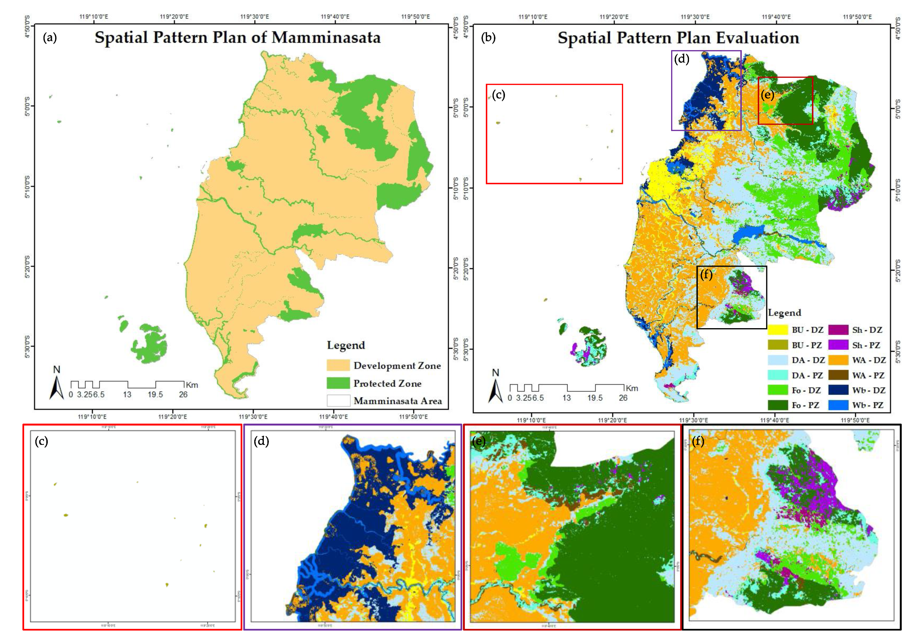
3.3. Comparison with the Spatial Plan

The Indonesian Government created a spatial plan that consists of a spatial pattern map for 2011–2031. The spatial pattern map was constructed based on the actual land cover (when the map was made), the number and needs of the people (actual and future), Government policies, and analysis of the carrying capacity of the region. A spatial pattern is the distribution of land allocation in an area that includes a development zone and a protected zone [58]. A development zone is designated to be developed based on the conditions and potential of natural, human, and artificial resources, while a protected zone is designated to protect environmental sustainability, which includes natural and man-made resources [59].
The land cover prediction approach was not included in the spatial plan by the Government. Therefore, the land cover prediction for 2031 was overlaid with the Government’s spatial pattern map to provide a detailed land cover distribution in both the development and protected zones. This result could be helpful to the Government in considering future development in the Mamminasata area.

4. Results

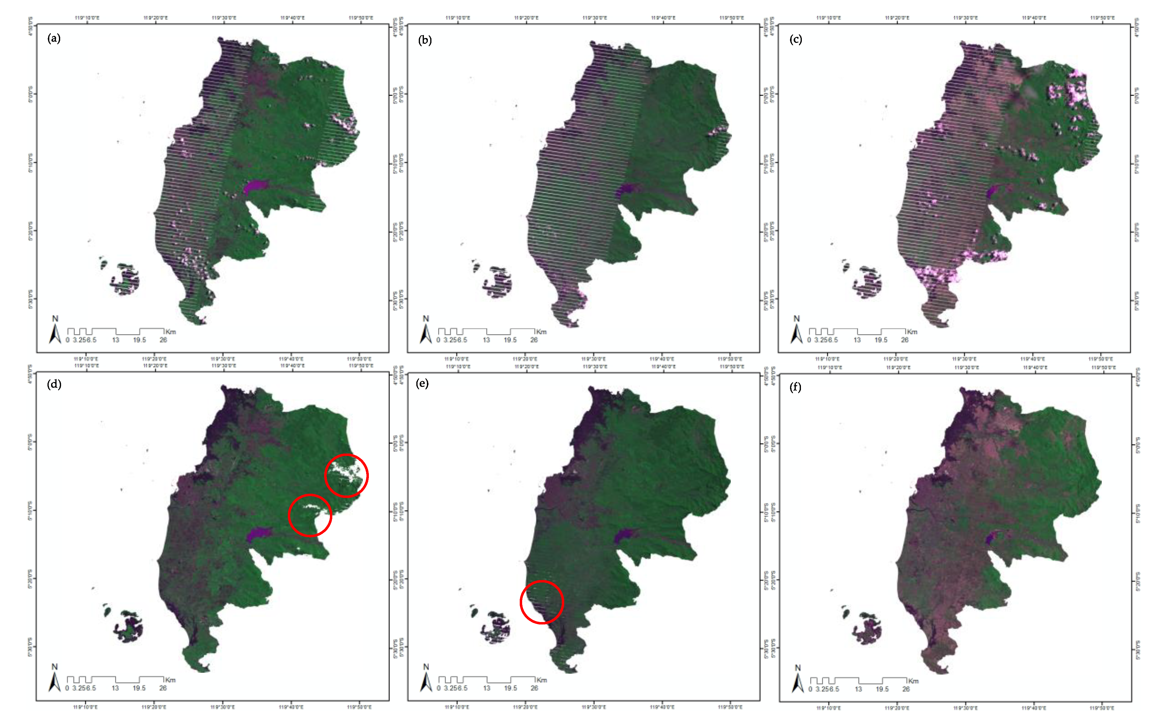
4.1. Land Cover Maps of 2006, 2011, and 2016

Figure 4 shows the three composite images used for the classification in 2011, together with single-date images before the composite. Cloud, shadow, and scan gaps before the composite were reduced, and smooth and clear scenes were produced by the composite.
Most of the pixels were composed of two base scenes that have the smallest seasonal change in step 1, and a small fraction of the pixels were filled by other scenes in step 2 (based on Table 2). Therefore, the appearances were smoother than the simultaneous composite of all the scenes. However, there were still white areas (no-data, marked by red circles) because there was no valid data in any of the scenes due to the clouds and scan gaps.
The center panel in Figure 5 is the land cover in 2011 generated by SVM classifier, showing that the obstacles (cloud, shadow, and scan-gap areas) can be overcome because the differences in the reflectance were small and dissolved through statistical grouping by the SVM classifier.
Table 4 shows the overall accuracy of land cover classification in 2011 was 0.83 with 600 points of total sample. The result indicated that the accuracy of land cover classification in 2011 was acceptable and can be used for land change modeling.
The land cover maps in 2006 and 2016 were obtained based on the change detection with 2011. The thresholds of change for normalized difference were 2.5 and 3.5 for respective years, determined by the visual comparison using a time series of Google Earth fine-resolution satellite images. As a result, total change areas were 4556 ha during 2006 to 2011, and 1301 ha during 2011 to 2016. The typical changed area of the final images can be seen in Figure 5. On the left side, some waterbody and wetland agriculture changed into built-up area; on the right side, some waterbody and shrub changed into dryland and wetland agriculture.

4.2. Land Cover Change Model

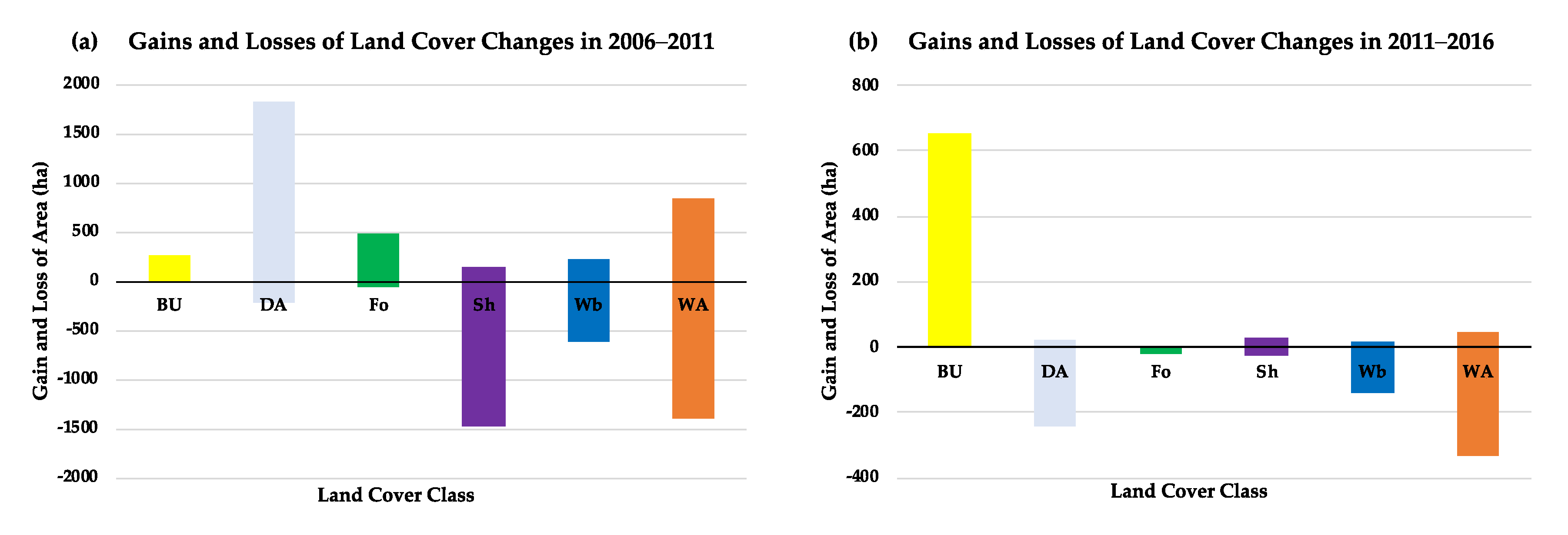
4.2.1. Land Cover Change Analysis

Figure 6 shows the gains and losses of land cover for two periods from 2006 to 2011 and from 2011 to 2016. In the analysis, there was no possibility of transition from built-up area to other classes, whereas other types of land cover had transitions between one another. Between 2006 and 2011, around 195 ha of wetland agriculture changed into built-up area, while dryland agriculture increased mainly from wetland agriculture (893 ha), shrub (746 ha), and waterbody (122 ha). In the same period, forest area increased, which was mostly obtained from shrub (347 ha). It can be seen that around 1472 ha shrub, 620 ha waterbody, and 1394 ha wetland agriculture changed into other types. However, there was an increase of around 843 ha of wetland agriculture from dryland agriculture, shrub, and waterbody. In the period between 2011 and 2016, the built-up area increased by 295 ha from wetland agriculture, 194 ha from dryland agriculture, and 130 ha from waterbody. This change is most likely because the Government program started during this period.

4.2.2. Land Cover Change Modeling

The seven driving factors are shown in Figure 7. Based on the relationship between driving factors and land cover in 2006–2011 using Cramer’s V test (Table 5), the highest and lowest influential factors were population density per pixel and distance from river and lake, respectively. It is reasonable that population density has a greater effect on land cover change, especially for agricultural and residential types of land cover. It is also natural that distance from water has less effect because many small rivers densely covered this area (as shown in Figure 7b), and enough water is available throughout the site.
The transition potential was obtained with 33.56% accuracy by running the MLPNN method from a combination of the basic maps (2006 and 2011) and the seven driving factors. This transition potential was used to simulate the land cover prediction for 2016 by using the MC method, and the resulting map is shown in Figure 8b.
After the land cover for 2016 was predicted, the resulting map was compared with the actual land cover map of 2016. Figure 8 shows the actual and predicted land cover for 2016 and the comparison of land cover classes between the two maps expressed as percentages. The two maps had almost the same values for all classes. The area of different land cover was 3125 ha.
Figure 9a shows the visual validation of the land cover prediction for 2016, displaying the four types of correctness and error: 0.00% hits, 98.89% null successes, 0.86% false alarms, and 0.25% misses. The correctness value (hits and null successes) indicated the same type of land cover between the actual map and the prediction map for 2016 (98.89%). Conversely, the error value (false alarms and misses) indicated the different types of land cover between the two maps (1.11%).
Statistical validation was carried out by comparing the whole area and different areas (areas of false alarms and misses). Table 6 shows the kappa values for the validation of the whole area and different areas. Pontius and Millones [60] revealed that the values of kappa for no information and grid-cell level location were somewhat more helpful than the values of kappa for stratum-level location and standard. Based on that, the results of accuracy can be accepted, and the model can be run for land cover prediction for 2031.

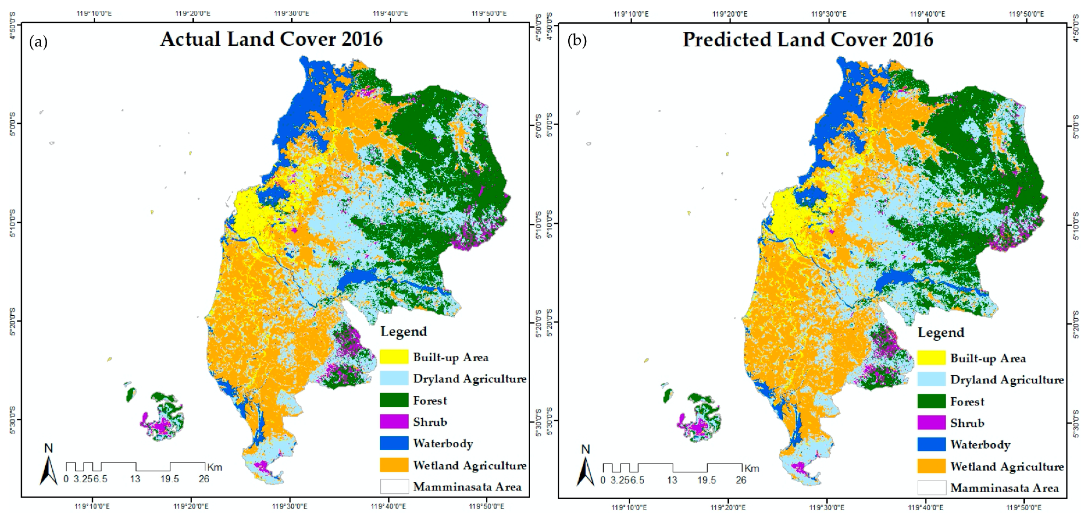
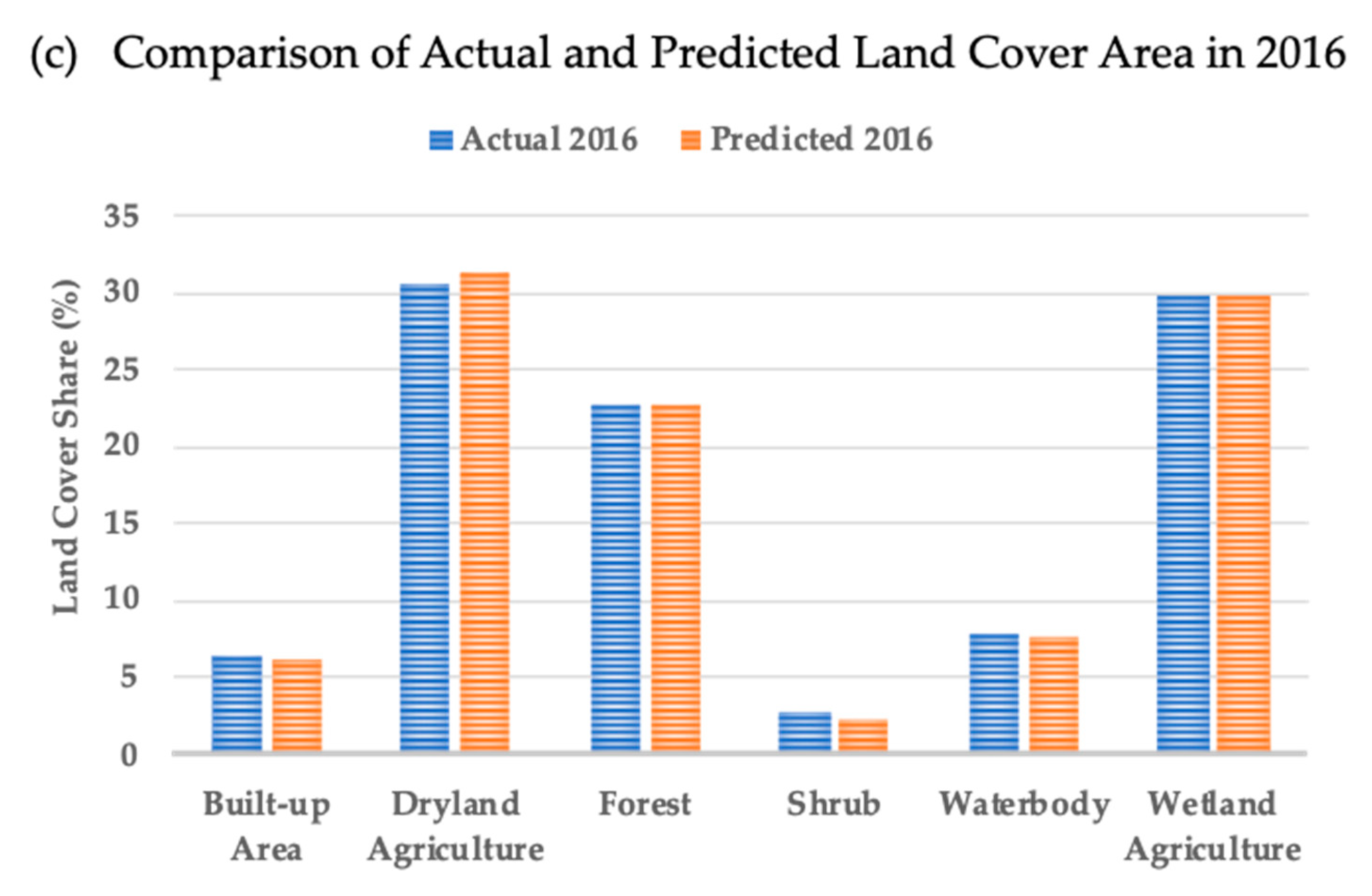
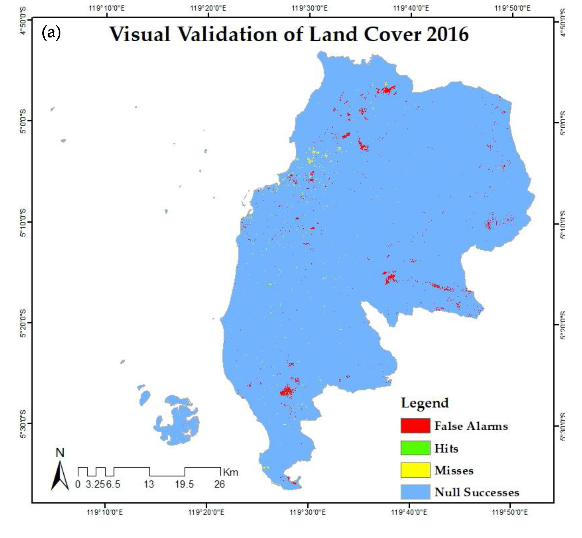
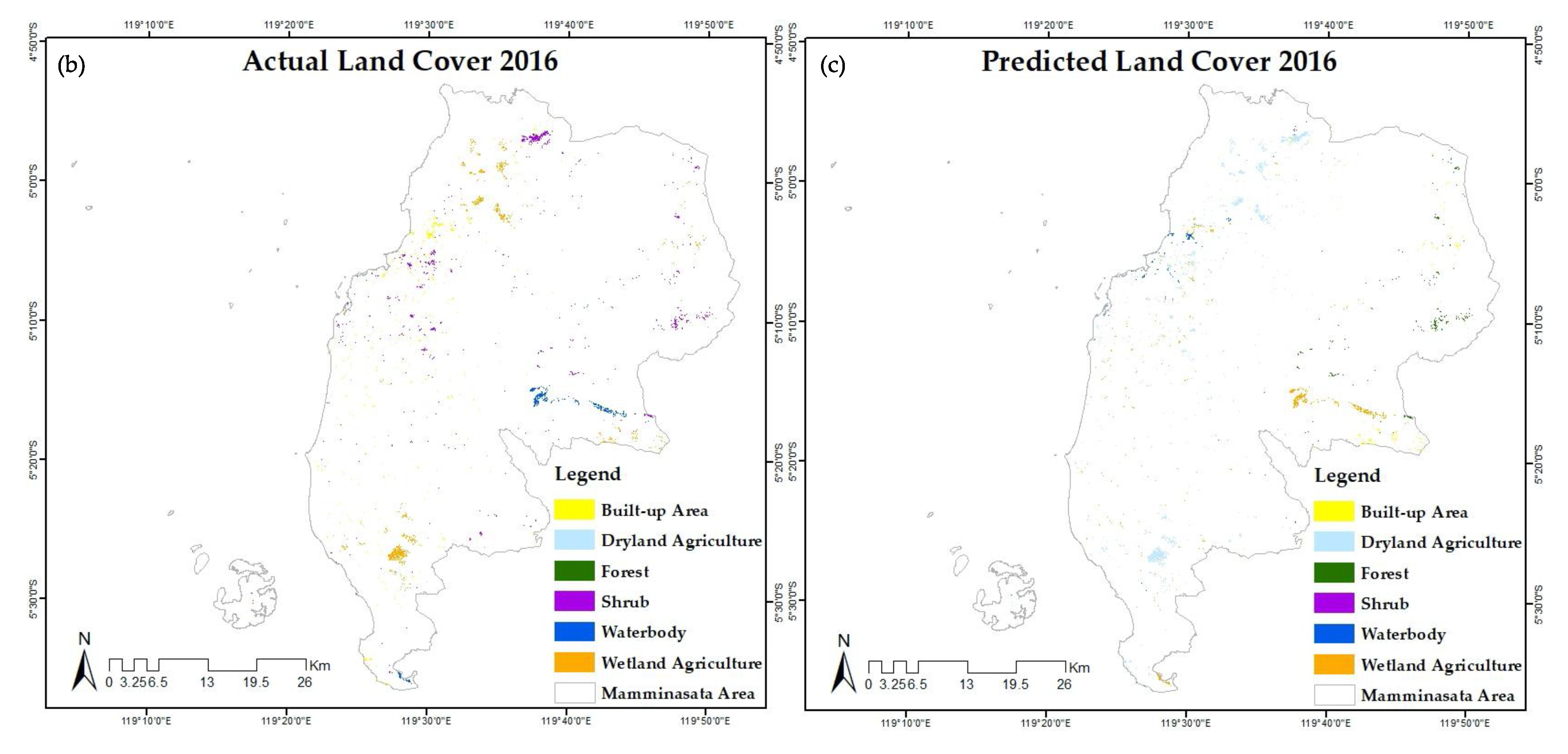
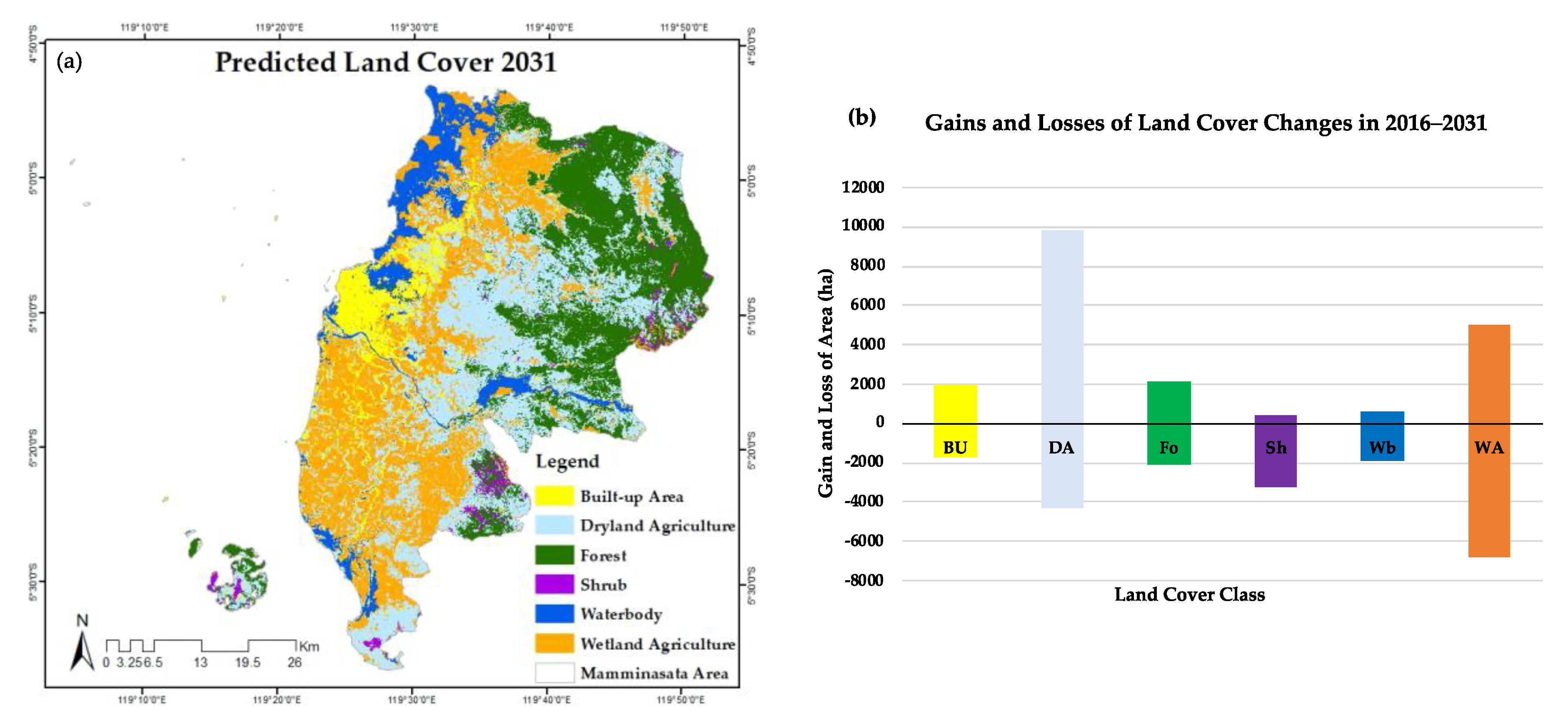
4.2.3. Land Cover Prediction for 2031

Figure 10a is the predicted land cover for 2031. The MC method was used with the same rules, seven driving factors, and basic maps (2006–2011) to predict land cover changes for 2031. Figure 10b shows the increases predicted for built-up area (252 ha), dryland agriculture (5578 ha), and forest (73 ha), and the decreases for shrub (2829 ha), waterbody (1282 ha), and wetland agriculture (1791 ha). Based on this prediction model, all types of land cover would have a transition potential between one another, including the built-up area, which did not experience a transition to other types of land cover in the period 2006–2016.

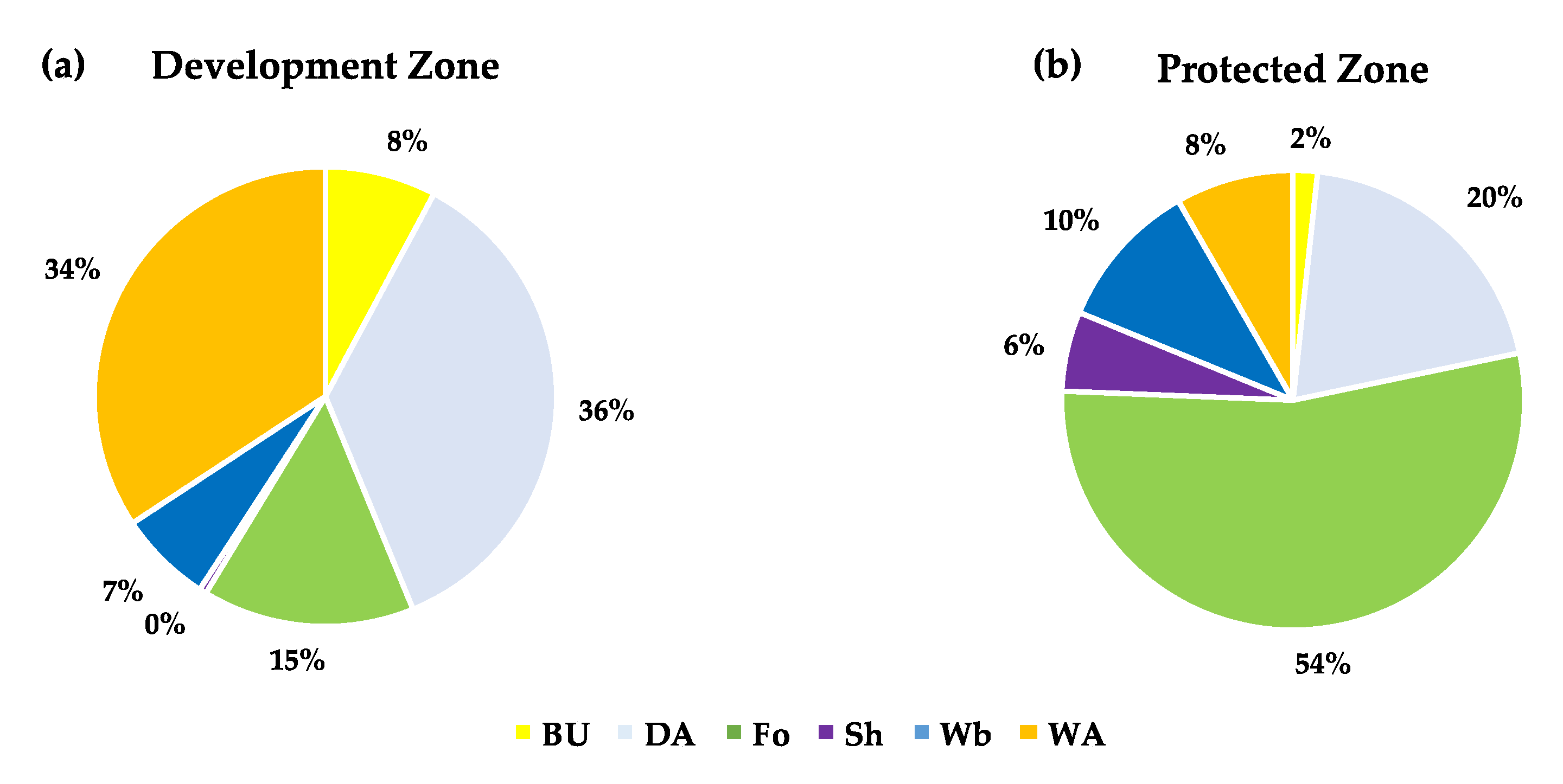
4.3. Comparing with the Spatial Plan

In the spatial pattern map from the Government, the total area of Mamminasata is divided into 80% development zone and 20% protected zone (Figure 11a). This map was overlaid with the land cover prediction map for 2031 to evaluate the Mamminasata spatial pattern (Figure 11b). The result shows that agricultural areas and waterbody occupy 70 and 7% of the development zone, respectively (Figure 12a), while 2% of the protected zone would become built-up area (Figure 12b).
The evaluation map also shows the small islands of Mamminasata called Spermonde, which are in the protected zone predicted to become built-up area (Figure 11c). Figure 11d shows waterbody in the development zone. The forest area occupies 15% of the development zone, mainly in the eastern and north-eastern parts of Mamminasata (Figure 11e,f). These areas are distant from the developed center, so special care is necessary to achieve sustainable development. Each land cover type in the development zone has a high possibility of changing into another land cover type in the future because the development zone is designed to be developed [59].

5. Discussion

In this section, we would like to address a few points based on our research aims. First, we have described a simple composite method to overcome the SLC problem of Landsat ETM+ coupled with the presence of cloud and shadow areas. This method proved to be useful in overcoming those obstacles in image processing. The land cover classification using the SVM classifier produced a precise land cover map with acceptable accuracy. The land cover classification map for 2011 using the SVM classifier in this study was helped by the availability of land use maps from the Government. We used this data as a training sample with the purpose of creating a land cover classification map without making new training data based on the visual interpretation of Landsat images.
As explained by Hussain et al. [44], the pixel-based technique using an algebra-based approach (image differencing) in this study has proven to be simple and easy to interpret. This technique is suitable for medium-resolution images such as those provided by Landsat. Based on the land cover maps of 2006 and 2016 shown in Figure 5 and the statistics in Figure 8, this technique helped us to detect an appropriate change in land cover. Our change detection method could be applied for another geographic scales and spatial resolutions if multispectral satellite data are available because the methodology is quite simple and general. Land cover is considerably complex with small patches in Asian countries, hence finer spatial resolution is preferable in order to reduce the mixture of land cover within a pixel. MultiSpectral Instrument (MSI) onboard the Sentinel-2 satellite would be a possible alternative because it has been operated continuously since 2015.
Although MLPNN showed a lower accuracy of transition potential than 80%, which is proposed by several researchers [10,11,50], our land cover prediction model for 2016 using the MC method showed the acceptable accuracy validated visually and statistically. Therefore, we would like to emphasize that MLPNN is a powerful method for modeling transition potential of land cover. It should be noted that our model only used current population and physical factors as driving factors. The economic factor was not included due to the unavailability of this data. Several researchers have proposed the economic factor in their land cover change model [11,61,62]. For further research, the economic factor should be selected into the model. All type of driving factor data (physical and socio-economic factors) could be included in the LCM. Furthermore, the influence order of driving factors will be determined using Cramer’s V.
Land cover prediction is not included in the current spatial plan in the study area. Therefore, the result of this study might be informative for current and future perspectives of the site. The importance of our result lies in the evaluation of the spatial pattern plan based on the land cover prediction. The evaluation map helped us to generate the detailed land cover distribution in both the development zone and the protected zone for 2031. Our model predicted that 30% of the protected zone would become built-up and agricultural areas, while forest accounted for 15% of the development zone. These conditions should be controlled by regulations in consideration of an unpredictable increase in population.
In reality, investment in land plots by both companies and individuals is also increasing rapidly with the establishment of Mamminasata as a national strategic area. Many agricultural, shrub, and waterbody (pond) areas have been converted into built-up areas, mainly residential and industrial areas, to meet the needs of the increasing population. Although the increase in built-up area cannot be avoided, adequate density and distribution should be considered together with environmental conservation.
Some regulations have already been enacted, for example, Indonesian Regulation No. 41 in 2009 (Protection for Sustainable Agriculture Land). Such regulations are needed because as an agrarian country, Indonesia needs to guarantee the provision of sustainable agricultural land as a source of work and decent livelihood for people by promoting the principles of togetherness, sustainability, environmental insight, etc., together with maintaining balance, progress, and national economic unity [63]. Indonesian Regulations (such as No. 41 in 1999 for Forestry, No. 17 in 2019 for Water Resources, and No. 26 in 2007 for Spatial Planning) are worthwhile and should be effectively put into practice. The evaluation map of the spatial pattern in this research could be used as guidance for the Government to apply these regulations to protect the conservation and hazardous areas.
In addition, local governments of the four municipalities in Mamminasata could cooperate to achieve common goals for development by balancing the development and the protected zones. Moreover, the National Government should strictly control investment in land plots to avoid the negative effects of the expansion of built-up areas. Managing the use of the Mamminasata area must be directed by zoning regulations, licensing, setting incentives and disincentives, and imposing sanctions for violations committed by any party. These actions should help to achieve sustainable development of the Mamminasata area.

6. Conclusions

Land cover of Mamminasata, Indonesia, in 2031 was predicted by the land cover change model using remote sensing and other geospatial data, and the resulting map was used to evaluate the spatial plan. The combination of predicted land cover and spatial plan helped to create a detailed map of future land cover in the development and protected zones. Significant land cover changes were expected in all four municipalities along with the increase in population density. The built-up area in the protected zone accounts for 2% of the total and agricultural areas would be 28% in 2031.
In terms of methodology, we found that the composite and change detection methods were simple and easy to follow. In addition, we showed that SVM is a powerful land cover classifier and useful even for medium-resolution images such as those provided by Landsat, and MLPNN + MC provides a good result in modeling land cover change prediction. It should be noted that the lower accuracy of transition potential in MLPNN could produce a good prediction of land cover, which was shown by the acceptable accuracy from the MC method (land cover prediction for 2016) validated by the actual land cover in 2016. This result is likely because the number of sub-models can affect the accuracy. Moreover, the transition potential accuracy in MLPNN should work well in most instances using default setting. As a suggestion, by experimenting the number of hidden layer nodes and the learning rate values in MLPNN as the two most critical parameters, it will affect the accuracy substantially.
Another topic that should be considered in further research is the prediction of population because land cover change is related to the needs of increased population, and the number of people can affect the carrying capacity of a region. These three topics are important in a spatial plan.
From our research, we suggest that the protected zone should be maintained or evenly expanded because Mamminasata is the economic center area in Eastern Indonesia coupled with its function as a national strategic area, which could result in an increase in population. Therefore, land cover prediction should be helpful in formulating a spatial plan, especially a spatial pattern plan to achieve goals for sustainable development.

Author Contributions

Conceptualization, Andi Muhammad Yasser Hakim, Sumbangan Baja, Dorothea Agnes Rampisela, and Samsu Arif; Methodology, Andi Muhammad Yasser Hakim and Masayuki Matsuoka; software, Andi Muhammad Yasser Hakim and Masayuki Matsuoka; Validation, Andi Muhammad Yasser Hakim and Masayuki Matsuoka; formal analysis, Andi Muhammad Yasser Hakim and Masayuki Matsuoka; investigation, Andi Muhammad Yasser Hakim and Masayuki Matsuoka; resources, Andi Muhammad Yasser Hakim, Masayuki Matsuoka, and Samsu Arif; data curation, Andi Muhammad Yasser Hakim, Masayuki Matsuoka, and Samsu Arif; writing—original draft preparation, Andi Muhammad Yasser Hakim; writing—review and editing, all authors; visualization, Andi Muhammad Yasser Hakim and Masayuki Matsuoka; Supervision, Masayuki Matsuoka, Sumbangan Baja, Dorothea Agnes Rampisela, and Samsu Arif; project administration, Sumbangan Baja and Dorothea Agnes Rampisela; funding acquisition, Sumbangan Baja. All authors have read and agreed to the published version of the manuscript.

Funding

This research was funded by the Indonesian Ministry of Research, Technology, and Higher Education, Grant No. 1739/UN4.21/PL.00.00/2019.

Acknowledgments

The GIS data were provided by the Centre for Regional Development and Spatial Information (WITaRIS), Hasanuddin University.

Conflicts of Interest

The authors declare no conflict of interest.

References

  1. United Nations. Agenda 21. In Proceedings of the United Nations Conference on Environment & Development, Rio de Janerio, Brazil, 3–14 June 1992; pp. 1–351. [Google Scholar]
  2. Purvis, B.; Mao, Y.; Robinson, D. Three pillars of sustainability: In search of conceptual origins. Sustain. Sci. 2018, 14, 681–695. [Google Scholar] [CrossRef] [Green Version]
  3. Scott, G.; Rajabifard, A. Sustainable development and geospatial information: A strategic framework for integrating a global policy agenda into national geospatial capabilities. Geo-Spat. Inf. Sci. 2017, 20, 59–76. [Google Scholar] [CrossRef] [Green Version]
  4. Hsu, S.; Perry, N. Sustainable Development in Malaysia and Indonesia; Palgrave Macmillan: New York, NY, USA, 2015; ISBN 9781137353078. [Google Scholar]
  5. Japan International Cooperation Agency: KRI International Corp.: Nippon Koei Co. Ltd. The Study on Implementation of Integrated Spatial Plan for The Mamminasata Metropolitan Area, South Sulawesi Province in Indonesia Final Report: Sector Study Report. 2006. Available online: https://openjicareport.jica.go.jp/340/340/340_108_11834108.html (accessed on 27 July 2020).
  6. García-Ruiz, J.M.; Lasanta, T.; Ruiz-Flano, P.; Ortigosa, L.; White, S.; González, C.; Martí, C. Land-use changes and sustainable development in mountain areas: A case study in the Spanish Pyrenees. Landsc. Ecol. 1996, 11, 267–277. [Google Scholar] [CrossRef]
  7. Musa, S.I.; Hashim, M.; Reba, M.N.M. Geospatial modelling of urban growth for sustainable development in the Niger Delta Region, Nigeria. Int. J. Remote Sens. 2018, 40, 1–29. [Google Scholar] [CrossRef]
  8. Salazar, E.; Henríquez, C.; Sliuzas, R.; Qüense, J. Evaluating spatial scenarios for sustainable development in Quito, Ecuador. ISPRS Int. J. Geo-Inf. 2020, 9, 141. [Google Scholar] [CrossRef] [Green Version]
  9. Sohl, T.; Wimberly, M.C.; Radeloff, V.C.; Theobald, D.M.; Sleeter, B.M. Divergent projections of future land use in the United States arising from different models and scenarios. Ecol. Model. 2016, 337, 281–297. [Google Scholar] [CrossRef] [Green Version]
  10. Chim, K.; Tunnicliffe, J.; Shamseldin, A.Y.; Ota, T. Land use change detection and prediction in Upper Siem Reap River, Cambodia. Hydrology 2019, 6, 64. [Google Scholar] [CrossRef] [Green Version]
  11. Losiri, C.; Nagai, M.; Ninsawat, S.; Shrestha, R.P. Modeling urban expansion in bangkok metropolitan region using demographic–economic data through cellular Automata-Markov chain and multi-layer perceptron-Markov chain models. Sustainability 2016, 8, 686. [Google Scholar] [CrossRef] [Green Version]
  12. Roy, H.G.; Fox, D.M.; Emsellem, K. Predicting land cover change in a mediterranean catchment at different time scales. Lect. Notes Comput. Sci. 2014, 8582, 315–330. [Google Scholar] [CrossRef]
  13. Pérez-Vega, A.; Mas, J.-F.; Ligmann-Zielinska, A. Comparing two approaches to land use/cover change modeling and their implications for the assessment of biodiversity loss in a deciduous tropical forest. Environ. Model. Softw. 2012, 29, 11–23. [Google Scholar] [CrossRef]
  14. Ozturk, D. Urban growth simulation of Atakum (Samsun, Turkey) using cellular Automata-Markov chain and multi-layer perceptron-Markov chain models. Remote Sens. 2015, 7, 5918–5950. [Google Scholar] [CrossRef] [Green Version]
  15. Ibrahim-Mahmoud, M.; Duker, A.; Conrad, C.; Thiel, M.; Ahmad, H.S. Analysis of settlement expansion and urban growth modelling using geoinformation for assessing potential impacts of urbanization on climate in Abuja City, Nigeria. Remote Sens. 2016, 8, 220. [Google Scholar] [CrossRef] [Green Version]
  16. Pickard, B.R.; Gray, J.; Meentemeyer, R.K. Comparing quantity, allocation and configuration accuracy of multiple land change models. Land 2017, 6, 52. [Google Scholar] [CrossRef] [Green Version]
  17. Ahmed, B.; Ahmed, R. Modeling urban land cover growth dynamics using multi-temporal satellite images: A case study of Dhaka, Bangladesh. ISPRS Int. J. Geo-Inf. 2012, 1, 3–31. [Google Scholar] [CrossRef] [Green Version]
  18. Tewolde, M.G.; Cabral, P. Urban sprawl analysis and modeling in Asmara, Eritrea. Remote Sens. 2011, 3, 2148–2165. [Google Scholar] [CrossRef] [Green Version]
  19. Singh, S.; Reddy, C.S.; Pasha, S.V.; Dutta, K.; Saranya, K.; Satish, K.V. Modeling the spatial dynamics of deforestation and fragmentation using Multi-Layer Perceptron neural network and landscape fragmentation tool. Ecol. Eng. 2017, 99, 543–551. [Google Scholar] [CrossRef]
  20. Shade, C.; Kremer, P. Predicting land use changes in Philadelphia following green infrastructure policies. Land 2019, 8, 28. [Google Scholar] [CrossRef] [Green Version]
  21. Mountrakis, G.; Im, J.; Ogole, C. Support vector machines in remote sensing: A review. ISPRS J. Photogramm. Remote Sens. 2011, 66, 247–259. [Google Scholar] [CrossRef]
  22. Coppin, P.; Jonckheere, I.; Nackaerts, K.; Muys, B.; Lambin, E. Digital change detection methods in ecosystem monitoring: A review. Int. J. Remote Sens. 2004, 25, 1565–1596. [Google Scholar] [CrossRef]
  23. Bruzzone, L.; Prieto, D. Automatic analysis of the difference image for unsupervised change detection. IEEE Trans. Geosci. Remote Sens. 2000, 38, 1171–1182. [Google Scholar] [CrossRef] [Green Version]
  24. Yuan, J.; Lv, X.; Dou, F.; Yao, J. Change analysis in urban areas based on statistical features and temporal clustering using TerraSAR-X time-series images. Remote Sens. 2019, 11, 926. [Google Scholar] [CrossRef] [Green Version]
  25. Malila, W.A. Change vector analysis: An approach for detecting forest changes with Landsat. Mach. Process. Remote Sensed Data Symp. 1980, 326–335. [Google Scholar]
  26. Noi, P.T.; Kappas, M. comparison of random forest, k-nearest neighbor, and support vector machine classifiers for land cover classification using Sentinel-2 imagery. Sensors 2017, 18, 18. [Google Scholar] [CrossRef] [Green Version]
  27. Lee, J.; Cardille, J.A.; Coe, M.T. Agricultural expansion in Mato Grosso from 1986–2000: A Bayesian time series approach to tracking past land cover change. Remote Sens. 2020, 12, 688. [Google Scholar] [CrossRef] [Green Version]
  28. Baeza, S.; Paruelo, J.M. Land use/land cover change (2000–2014) in the Rio de la Plata Grasslands: An analysis based on MODIS NDVI Time Series. Remote Sens. 2020, 12, 381. [Google Scholar] [CrossRef] [Green Version]
  29. Zhou, Q.; Tollerud, H.J.; Barber, C.P.; Smith, K.; Zelenak, D. Training data selection for annual land cover classification for the land change monitoring, assessment, and projection (LCMAP) initiative. Remote Sens. 2020, 12, 699. [Google Scholar] [CrossRef] [Green Version]
  30. Jozdani, S.E.; Johnson, B.A.; Chen, D. Comparing deep neural networks, ensemble classifiers, and support vector machine algorithms for object-based urban land use/land cover classification. Remote Sens. 2019, 11, 1713. [Google Scholar] [CrossRef] [Green Version]
  31. Sharma, R.; Nehren, U.; Rahman, S.A.; Meyer, M.; Rimal, B.; Seta, G.A.; Baral, H. Modeling land use and land cover changes and their effects on biodiversity in Central Kalimantan, Indonesia. Land 2018, 7, 57. [Google Scholar] [CrossRef] [Green Version]
  32. Liping, C.; YuJun, S.; Saeed, S. Monitoring and predicting land use and land cover changes using remote sensing and GIS techniques—A case study of a hilly area, Jiangle, China. PLoS ONE 2018, 13, e0200493. [Google Scholar] [CrossRef]
  33. Turner, W.; Rondinini, C.; Pettorelli, N.; Mora, B.; Leidner, A.; Szantoi, Z.; Buchanan, G.; Dech, S.; Dwyer, J.L.; Herold, M.; et al. Free and open-access satellite data are key to biodiversity conservation. Biol. Conserv. 2015, 182, 173–176. [Google Scholar] [CrossRef] [Green Version]
  34. Central Bureau of Statistics. Gross Regional Domestic Product 2010; BPS Sulawesi Selatan: Makassar, Indonesia, 2011. (In Indonesian)
  35. Central Bureau of Statistics. Gross Regional Domestic Product of Regency/City in South Sulawesi 2011–2015; BPS Sulawesi Selatan: Makassar, Indonesia, 2016; ISBN 9786026426055. (In Indonesian)
  36. Central Bureau of Statistics. Gross Regional Domestic Product of Regency/City in South Sulawesi 2014–2018; BPS Sulawesi Selatan: Makassar, Indonesia, 2019; ISBN 9786026426840. (In Indonesian)
  37. Presidential Regulation No. 55. Spatial Plan of Makassar, Maros, Sungguminasa and Takalar Urban Area; Sekretariat Kabinet Republik Indonesia: Jakarta, Indonesia, 2011. (In Indonesian) [Google Scholar]
  38. United States Geological Survey (USGS). Earth Explorer. Available online: http://earthexplorer.usgs.gov (accessed on 19 November 2019).
  39. Fisher, A.G. Cloud and cloud-shadow detection in SPOT5 HRG imagery with automated morphological feature extraction. Remote Sens. 2014, 6, 776–800. [Google Scholar] [CrossRef] [Green Version]
  40. Zhu, X.; Liu, D.; Chen, J. A new geostatistical approach for filling gaps in Landsat ETM+ SLC-off images. Remote Sens. Environ. 2012, 124, 49–60. [Google Scholar] [CrossRef]
  41. Yin, G.; Mariethoz, G.; McCabe, M. Gap-filling of Landsat 7 imagery using the direct sampling method. Remote Sens. 2016, 9, 12. [Google Scholar] [CrossRef] [Green Version]
  42. Huang, K.-C.; Huang, T.C.C. Simulation of land-cover change in Taipei metropolitan area under climate change impact. IOP Conf. Ser. Earth Environ. Sci. 2014, 18, 12106. [Google Scholar] [CrossRef] [Green Version]
  43. Pal, M.; Mather, P.M. Support vector machines for classification in remote sensing. Int. J. Remote Sens. 2005, 26, 1007–1011. [Google Scholar] [CrossRef]
  44. Hussain, M.; Chen, D.M.; Cheng, A.; Wei, H.; Stanley, D. Change detection from remotely sensed images: From pixel-based to object-based approaches. ISPRS J. Photogramm. Remote Sens. 2013, 80, 91–106. [Google Scholar] [CrossRef]
  45. Aruna, S.; Rajagopalan, S. A novel SVM based CSSFFS feature selection algorithm for detecting breast cancer. Int. J. Comput. Appl. 2011, 31, 14–20. [Google Scholar]
  46. Parikh, K.S.; Shah, T.P. Support vector machine—A large margin classifier to diagnose skin illnesses. Procedia Technol. 2016, 23, 369–375. [Google Scholar] [CrossRef] [Green Version]
  47. Alimuddin, I. Irwan The application of Sentinel 2B satellite imagery using supervised image classification of maximum likelihood algorithm in landcover updating of the Mamminasata Metropolitan Area, South Sulawesi. IOP Conf. Ser. Earth Environ. Sci. 2019, 280, 1–8. [Google Scholar] [CrossRef]
  48. Asokan, A.; Anitha, J. Change detection techniques for remote sensing applications: A survey. Earth Sci. Inform. 2019, 12, 143–160. [Google Scholar] [CrossRef]
  49. Megahed, Y.; Cabral, P.; Silva, J.; Caetano, M. Land cover mapping analysis and urban growth modelling using remote sensing techniques in Greater Cairo Region—Egypt. ISPRS Int. J. Geo-Inf. 2015, 4, 1750–1769. [Google Scholar] [CrossRef] [Green Version]
  50. Eastman, J.R. Terrset-Manual; Clark Labs, Clark University: Worcester, MA, USA, 2016; p. 01610-1477. [Google Scholar]
  51. Pontius, R.G.; Boersma, W.; Castella, J.-C.; Clarke, K.C.; De Nijs, T.; Dietzel, C.; Duan, Z.; Fotsing, E.; Goldstein, N.; Kok, K.; et al. Comparing the input, output, and validation maps for several models of land change. Ann. Reg. Sci. 2007, 42, 11–37. [Google Scholar] [CrossRef] [Green Version]
  52. Central Bureau of Statistics. Sulawesi Selatan in Figures; BPS Sulawesi Selatan: Makassar, Indonesia, 2012. (In Indonesian)
  53. Alberto, A.; Dasanto, B.D. Model perubahan penggunaan lahan dan pendugaan cadangan karbon di daerah aliran sungai Cisadane, Jawa Barat Landuse change model and carbon stock estimation in Cisadane Watershed, West Java. Agromet 2010, 24, 18–26. [Google Scholar] [CrossRef]
  54. Lay, U.S.; Pradhan, B.; Yusoff, Z.; Abdullah, A.F.; Aryal, J.; Park, H.-J. Data mining and statistical approaches in debris-flow susceptibility modelling using airborne LiDAR data. Sensors 2019, 19, 3451. [Google Scholar] [CrossRef] [Green Version]
  55. Zubair, O.A.; Ji, W.; Weilert, T. Modeling the Impact of Urban Landscape Change on Urban Wetlands Using Similarity Weighted Instance-Based Machine Learning and Markov Model. Sustainability 2017, 9, 2223. [Google Scholar] [CrossRef] [Green Version]
  56. Nadoushan, M.A.; Soffianian, A.; Alebrahim, A. Predicting urban expansion in Arak Metropolitan Area using two land change models. World Appl. Sci. J. 2012, 18, 1124–1132. [Google Scholar] [CrossRef]
  57. Kim, I.; Jeong, G.; Park, S.; Tenhunen, J. Predicted land use change in the Soyang River Basin, South Korea. In Proceedings of the 2011 TERRECO Science Conference, Garmisch-Partenkirchen, Germany, 2–7 October 2011; pp. 17–24. [Google Scholar]
  58. Ministry of Agrarian and Spatial Planning Regulation No. 1. Spatial Plan Drafting Guidelines for Province, Regency and City; Sekretariat Kabinet Republik Indonesia: Jakarta, Indonesia, 2018. (In Indonesian)
  59. Indonesian Regulation No. 26. Spatial Plan; Sekretariat Kabinet Republik Indonesia: Jakarta, Indonesia, 2007. (In Indonesian) [Google Scholar]
  60. Pontius, R.G.; Millones, M. Death to Kappa: Birth of quantity disagreement and allocation disagreement for accuracy assessment. Int. J. Remote Sens. 2011, 32, 4407–4429. [Google Scholar] [CrossRef]
  61. Trisurat, Y.; Shirakawa, H.; Johnston, J.M. Land-use/land-cover change from socio-economic drivers and their impact on biodiversity in Nan province, Thailand. Sustainability 2019, 11, 649. [Google Scholar] [CrossRef] [Green Version]
  62. Ustaoglu, E.; Aydınoglu, A. Regional variations of land-use development and land-use/cover change dynamics: A case study of Turkey. Remote Sens. 2019, 11, 885. [Google Scholar] [CrossRef] [Green Version]
  63. Indonesian Regulation No. 41. Protection for Sustainable Agriculture Land; Sekretariat Kabinet Republik Indonesia: Jakarta, Indonesia, 2009. (In Indonesian) [Google Scholar]
Figure 1. Research site: (a) Indonesia; (b) South Sulawesi province; (c) Mamminasata area.
Ijgi 09 00481 g001
Figure 2. Land cover classification flowchart.
Ijgi 09 00481 g002
Figure 3. Land cover change modeling flowchart.
Ijgi 09 00481 g003
Figure 4. Landsat 7 ETM+ 2011: (a) scene 1 (11/04/2010), (b) scene 2 (03/07/2011), and (c) scene 3 (05/09/2011) before composite; (d) scene 1, (e) scene 2, and (f) scene 3 after composite. Note: red circles indicated no-data; bands 3, 4, and 2 were used for red, green, and blue, respectively.
Ijgi 09 00481 g004
Figure 5. Land cover classification: (a,c,f) 2011 using a support vector machine (SVM) classifier; (b,e) 2006 using change detection; and (d,g) 2016 using change detection.
Ijgi 09 00481 g005
Figure 6. Land cover changes of the research site: (a) in 2006–2011; (b) in 2011–2016. Note: BU—built-up area; DA—dryland agriculture; Fo—forest; Sh—shrub; Wb—waterbody; and WA—wetland agriculture.
Ijgi 09 00481 g006
Figure 7. Driving factor maps: (a) distance from capital, (b) distance from river and lake, (c) distance from road, (d) distance from settlement, (e) elevation, (f) slope, and (g) population density per pixel. Distances and elevation are in meters, slope is in degrees, and population density per pixel is in people/km2.
Ijgi 09 00481 g007aIjgi 09 00481 g007b
Figure 8. Actual land cover derived by satellite data (a); predicted land cover by multi-layer perceptron neural network and the Markov chain (MLPNN + MC) (b); comparison of land cover area (c).
Ijgi 09 00481 g008aIjgi 09 00481 g008b
Figure 9. Visual validation (a); actual (b) and predicted land cover maps for 2016 for different areas (c).
Ijgi 09 00481 g009aIjgi 09 00481 g009b
Figure 10. Land cover prediction for 2031 (a); land cover changes distribution of the research site in 2016–2031. Note: BU—built-up area; DA—dryland agriculture; Fo—forest; Sh—shrub; Wb—waterbody; and WA—wetland agriculture (b).
Ijgi 09 00481 g010
Figure 11. Spatial pattern plan from the Government (a); spatial pattern plan evaluation (b); Spermonde islands (c); waterbody area (d); forest area (e); and shrub area (f). Note: BU—built-up area; DA—dryland agriculture; Fo—forest; Sh—shrub; Wb—waterbody; WA—wetland agriculture; DZ—development zone; and PZ—protected zone.
Ijgi 09 00481 g011
Figure 12. Percentage of land cover area in 2031: (a) in the development zone; (b) in the protected zone. Note: BU—built-up area; DA—dryland agriculture; Fo—forest; Sh—shrub; Wb—waterbody; and WA—wetland agriculture.
Ijgi 09 00481 g012
Table 1. Observation dates of Landsat in three periods.
YearSatellite and SensorObservation Dates
2006Landsat 7 ETM+15/05/200521/07/2006
11/02/200607/09/2006
2011Landsat 7 ETM+10/03/201021/09/2011
11/04/201031/03/2012
27/04/201009/10/2012
29/05/201018/03/2013
02/09/201022/06/2013
13/03/201108/07/2013
16/05/201125/08/2013
03/07/201126/09/2013
05/09/2011
2016Landsat 8 OLI15/02/201624/07/2016
05/05/201610/09/2016
Table 2. List of composite scenes.
Scene 1Scene 2Scene 3
Step 111/04/2010
27/04/2010
03/07/2011
22/06/2013
05/09/2011
21/09/2011
Step 216/05/2011
13/03/2011
31/03/2012
10/03/2010
18/03/2013
29/05/2010
08/07/2013
02/09/2010
25/08/2013
09/10/2012
26/09/2013
02/09/2010
25/08/2013
Table 3. List of image pairs.
20062016
12/02/2012–11/02/2006
16/05/2011–15/05/2005
03/07/2011–21/07/2006
05/09/2011–07/09/2006
12/02/2012–15/02/2016
16/05/2011–05/05/2016
03/07/2011–24/07/2016
05/09/2011–10/09/2016
Table 4. Confusion matrix.
Classification ClassTotal RowPA
BUDAFoShWbWA
Ground TruthBU8220110860.95
DA7670010750.89
Fo11229825341630.60
Sh0726302740.85
Wb02059321020.91
WA00062921000.92
Total Column100100100100100100600
UA0.820.670.980.630.930.92
OA0.83
AoC0.17
KC0.79
Note: BU—built-up area; DA—dryland agriculture; Fo—forest; Sh—shrub; Wb—waterbody; WA—wetland agriculture; PA—producer’s accuracy; UA—user’s accuracy; OA—overall accuracy; AoC—agreement of chance; and KC—kappa coefficient.
Table 5. Cramer’s V values of driving factors.
VariableOverall Cramer’s V
Distance from Capital0.3230
Distance from River and Lake0.1103
Distance from Road0.1965
Distance from Settlement0.2542
Elevation0.3263
Slope0.2888
Population Density per Pixel0.4920
Table 6. Accuracy test of change prediction.
Type of KappaKappa Value
Whole AreaDifferent Areas
No information0.99610.9973
Grid-cell level location0.99740.7821
Stratum-level location0.99740.7821
Standard0.99250.6544

