Characterisation of Indoor Massive MIMO Channels Using Ray-Tracing: A Case Study in the 3.2–4.0 GHz 5G Band


Departamento de Ingeniería de Comunicaciones, Universidad de Cantabria, 39005 Santander, Spain
*
Author to whom correspondence should be addressed.
Electronics 2020, 9(8), 1250; https://doi.org/10.3390/electronics9081250
Submission received: 23 June 2020
/
Revised: 29 July 2020
/
Accepted: 29 July 2020
/
Published: 4 August 2020
(This article belongs to the Special Issue Channel Characterization for Wireless and Mobile Communications)
Abstract
:In this paper, research results on the applicability of ray-tracing (RT) techniques to model massive MIMO (MaMi) channels are presented and discussed. The main goal is to show the possibilities that site-specific models based on rigorous RT techniques, along with measurement campaigns considered for verification or calibration purposes where appropriate, can contribute to the development and deployment of 5G systems and beyond using the MaMi technique. For this purpose, starting from the measurements and verification of the simulator in a symmetric, rectangular and accessible scenario used as the testbed, the analysis of a specific case involving channel characterisation in a large, difficult access and measurement scenario was carried out using the simulation tool. Both the measurement system and the simulations emulated the up-link in an indoor cell in the framework of a MaMi-TDD-OFDM system, considering that the base station was equipped with an array consisting of 10 × 10 antennas. The comparison of the simulations with the measurements in the testbed environment allowed us to affirm that the accuracy of the simulator was high, both for determining the parameters of temporal dispersion and frequency selectivity, and for assessing the expected capacity in a specific environment. The subsequent analysis of the target environment showed the high capacities that a MaMi system can achieve in indoor picocells with a relatively high number of simultaneously active users.
1. Introduction
Currently, the idea that the development and subsequent deployment of 5G and beyond communications systems requires an increasingly precise and complete characterisation and modelling of the radio channel is widely accepted. In recent years, significant efforts have been made to propose new channel models or to complete existing ones, especially to include multiple input–multiple output (MIMO) and massive MIMO (MaMi) modelling.
A widely accepted classification of channel models divides them into stochastics and determinists. As representative stochastic models, we can highlight the models derived from WINNER [1], QuaDRiGa [2] and COST2100 [3]. Concerning deterministic models, these are based on the electromagnetic propagation theory for the characterisation of radioelectric propagation.
Focusing on deterministic models, there are methods based on the full solution of Maxwell’s equations by numerical methods, such as the finite-difference time domain (FDTD) method [4]. These methods are numerically intensive and their application to systems with large arrays is not practicable today. However, high-frequency approaches for radio propagation are applicable in the frequency bands of current wireless systems, which together with ray-tracing techniques allow sufficiently accurate models of radio channels to be developed. Among other possibilities, the site-specific models which currently offer the most accurate results for micro and pico cells are those that—supported by ray-tracing techniques—implement the high-frequency propagation approach based on the combination of geometric optics with the uniform theory of diffraction (GO/UTD) [5,6,7].
Ray-tracing (RT) methods vary from one another depending on how the following fundamental tasks are solved: (1) finding the rays that connect the transmitter to the receiver in the most efficient way in a complex environment, in other words, ray-tracing, and (2) calculating as accurately as possible the electromagnetic field associated with such rays. There are multiple options for solving these two central aspects of the model, always seeking a balance between efficiency and accuracy. In [8], the reader can find an extensive tutorial that analyses these aspects in detail, their historical evolution and their current state. A selection and analysis of current commercial and academic RT-based simulators are also presented.
RT methods, used alone or as a complement to statistical channel models, present several advantages for the development and subsequent deployment of systems based on MaMi technology [8,9,10]. First, the use of large arrays results in a lack of stationarity of the channel along the antenna elements of the array that must be adequately modelled. This non-stationarity is fundamentally due to the appearance and disappearance of certain multipath components. This effect is strongly site-specific, and therefore its analysis by RT is highly adequate. Second, the characteristics of the MaMi channel matrix, specifically the degree of orthogonality of its columns, i.e., the degree to which the favourable propagation condition will be met, depends not only on the geometry of the environment but also on the relative position of active users. Again, this characteristic of the MaMi channel can be advantageously analysed with site-specific models. Third, propagation models based on RT provide information on the directions of arrival (DoA) and departure (DoD) of the multipath components. This information is one of the most complex to acquire through measurements.
The use of RT methods in conjunction with measurement campaigns would allow a full channel characterisation to be acquired. This more complete characterisation of the channel would be the input of stochastic models, obtaining from this hybrid approach the advantages of both types of models. Finally, it is also interesting to highlight the possibilities of analysing time-variation channels in dynamic scenarios where not only the Tx and Rx can be in motion, but also the objects in the environment [8].
From the point of view of the deployment of 5G networks, and in particular of MaMi systems, RT methods can be increasingly helpful. Apart from the classic coverage analysis, which is still of interest, there are many other important issues from the point of view of system engineering, for example, determining the optimal placement and tilt angle of the base station (BS) array in a complex environment. In addition, the selection of the type of antenna to be used as an elementary antenna of the array, depending on the type of coverage and environment, is also an important task. RT propagation modelling, integrated with optimisation tools, as heuristics methods, could play an important role in the optimum deployment of 5G systems [11].
The authors have recently contributed to the empirical characterisation of the massive MIMO channels by carrying out several measurement campaigns in the 3.5 GHz band [12,13,14]. Furthermore, they have broad experience in the development, validation and subsequent application of RT techniques in the deployment of wireless systems [11,15,16,17,18,19]. In [19], the authors showed the suitability of RT techniques to simulate point-to-point MIMO channels in indoor environments. In that work, point-to-point MIMO systems with a low number of antennas (2 × 2) were analysed. In this work, experimental capabilities were combined with RT experience to present a methodology for the characterisation of massive MIMO channels based on RT, supported by a measurement campaign.
The indoor environments and the frequency band considered (3.2 to 4.0 GHz) are both of interest, and the main intention is to show the abilities of the RT-based method. In fact, the achievable degree of accuracy is shown in detail and quantitatively, and the results obtained are supported with measurements carried out in a reference environment. This reference scenario is a medium size meeting room with structural characteristics and construction materials similar to the target scenario. Once the simulator was properly tested and its usefulness shown, the aim of the research was focused on simulating the MaMi channel in a target environment of interest, a large assembly hall in which it was not practical to carry out measurements with our experimental setup.
The rest of the paper is organised as follows. In Section 2, the methodology followed, the measurement system, the RT model as well as the basic parameters of the MaMi are presented. These parameters include the root mean square (RMS) delay spread and the coherence bandwidth, both related to the frequency selectivity of the channel, as well as the attainable sum capacity, used to characterise the MaMi system, defined within the TDD-OFDM operation framework. Section 3 outlines the results achieved and their discussion. Finally, the conclusions are summarised in Section 4.
2. Channel Characterisation: Methodology
In this work, the results of a channel measurement campaign carried out in an indoor scenario were considered as the testbed to calibrate and analyse the abilities of an academic RT-based tool [15,16,17,18]. Next, once the performance of the simulator was properly investigated, it was applied to characterise the indoor radio channel in a more complex environment, a large, stepped profile assembly hall in which it is difficult to undertake an empirical characterisation.
In this section, the main characteristics of both the channel measurement setup considered to perform the channel sounding, along with the software tool, are summarised.
2.1. The Measurement Setup
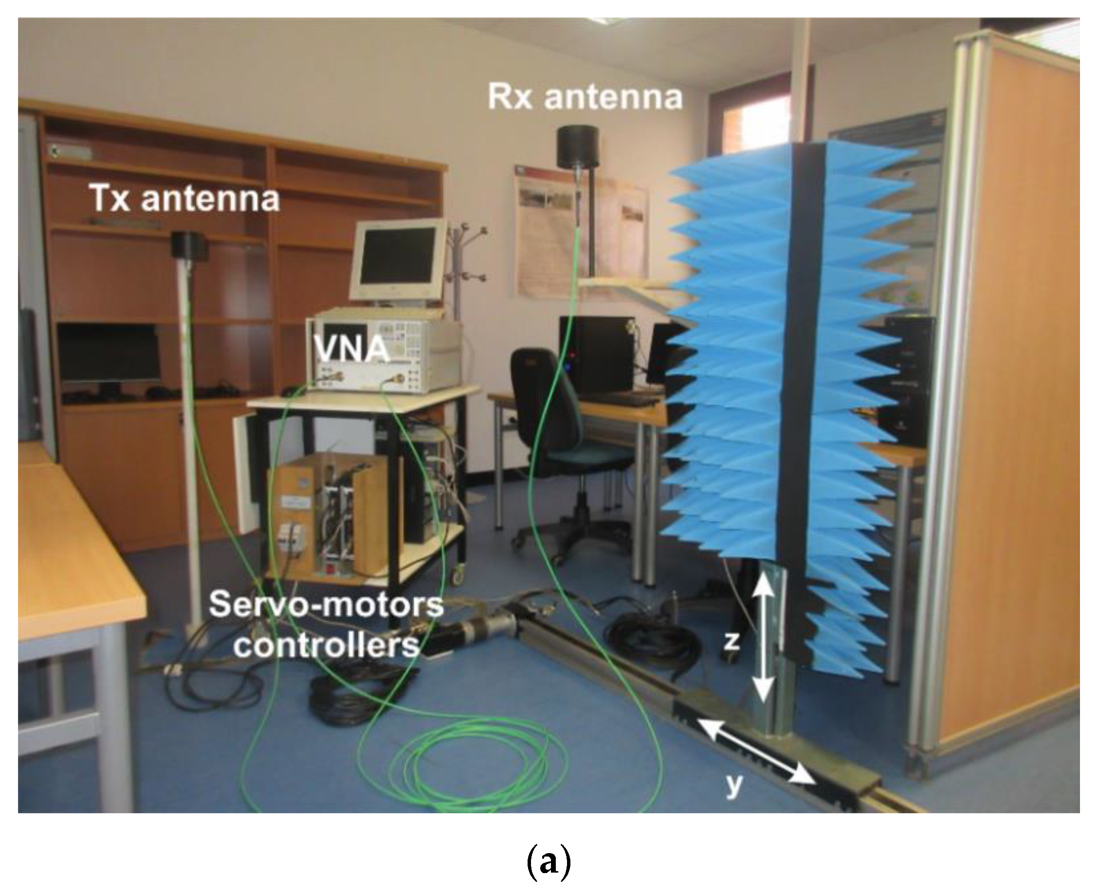
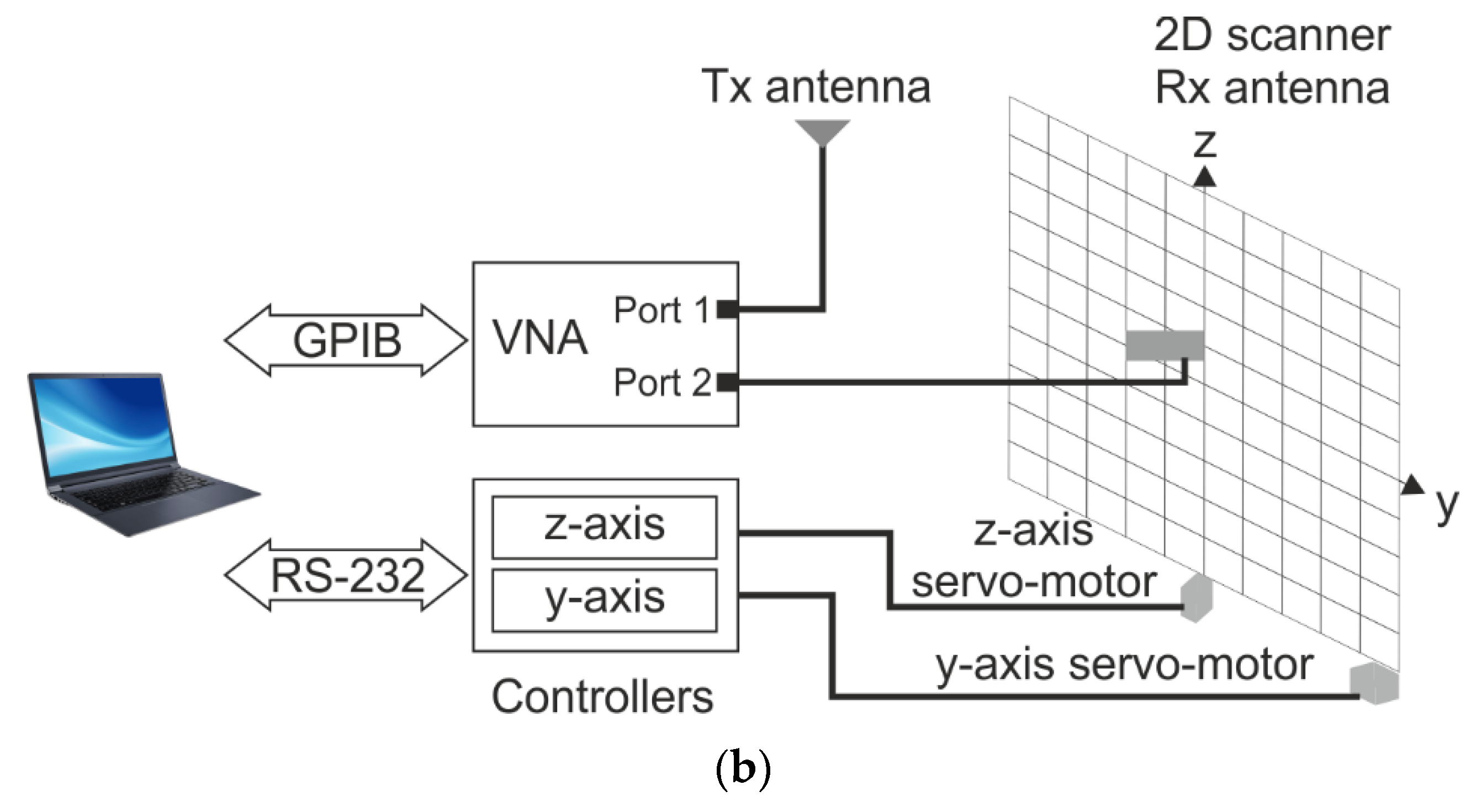
The channel sounding was carried out using the setup shown in Figure 1 [12,13]. Basically, and according to Figure 1a, it consisted of a planar scanner and a vector network analyser (VNA), the E8362A model from Keysight Technologies, both remote controlled from a computer to synchronously measure at any position in the frequency domain the S21(f) scattering parameter, i.e., a sampled version of the complex channel transfer function (CTF) [13].
From a mechanical point of view, and as depicted in Figure 1b, the 2D scanner consisted of two servo-motors that controlled the movement of the receiver antenna (Rx) over two linear units, considering that the Rx was properly fixed with a wooden mast to the vertical one. This made it possible for the Rx to be moved on a vertical plane emulating a virtual array (VA), acquiring remotely at each position of the YZ plane the S21-trace from the VNA. The post-processing of the -traces made it possible to obtain the CTF along with a characterisation of the up-link channel established between an active user terminal (UT), i.e., the transmitter antenna (Tx), and the array at the BS, i.e., the receiver VA.
Regarding the antennas used to carry out the measurements, two ultra-wideband antennas, both linearly polarised, were considered: the EM-6865 biconical omnidirectional antenna from Electrometrics as the Tx, and the HG2458-08LP log-periodic antenna from L-Com as the Rx. The EM-6865 operates in the range of 2–18 GHz and exhibits an average gain of 2.1 dBi in the 3.2–4 GHz frequency band of interest. Meanwhile, the HG2458-08LP operates in the range of 2.3–6.5 GHz, with an 8 dBi gain; a front to back ratio higher than 20 dB and vertical and horizontal beam widths of 60 and 80 degrees, respectively.
Focusing on the measurement settings, at any position of the 2D scanner, the S21(f) was measured considering Nf = 641 frequency tones Δf = 1.25 MHz uniformly spaced in the 3.2 to 4 GHz frequency range. As a result, a sampled version of the CTF was obtained for any Tx–Rx channel. The frequency resolution (Δf) used led to a maximum observable distance of 240 m (stated as c0/Δf, c0 being the speed of light), enough to guarantee that the multipath contributions were properly measured [13]. Finally, and concerning the 2D scanner, the Rx moved on the YZ plane, implementing a 10 × 10 uniform rectangular array (URA) with an inter-element separation in both directions of Δy = Δz = 50 mm and a total area of 0.2025 m2 for the URA. A summary with the main settings of the measurement campaign can be found in Table 1.
It should be noted that the influence of the presence of people on the channel performance is beyond the scope of this work and that the authors carried out channel measurements at night to guarantee stationary conditions.
2.2. The Ray-Tracing Model and Simulator Tool
High-frequency models, based on a 3D implementation of geometrical optics and uniform theory of diffraction (3D GO/UTD), can be considered a powerful tool for calculating signal levels in specific radio propagation environments [15,16,17]. The radio propagation process can be considered as a set of scattering mechanisms that contribute to electromagnetic fields, such as attenuation, transmission, reflection and diffraction. Each of these mechanisms has an associated ray, and the coupling between the transmit and receive antennas is obtained by the contribution of different rays, such as direct field, multiple reflections, single and double edge diffraction and combinations of diffraction–reflection and reflection–diffraction. The effect of the number of contributions included in the propagation can be quantified by the mean error and the standard deviation of errors [16,17].
The 3D GO/UTD model rigorously takes into account the orientation and radiation pattern of the transmit and receive antennas, as well as the polarisation of the signals. The application of a ray approach to the analysis of the radio propagation process is based on the assumption of a geometrical and electromagnetic model of the environment. A model constructed with flat facets to represent urban and indoor scenarios is highly suitable if we add some electrical parameters such as the relative dielectric constant, conductivity, the standard deviation of the surface roughness and the transmission coefficient or the wall width. The materials to model the obstacles were chosen in accordance with the real environment: limestone for the external walls, brick for the internal walls, wood for the doors, glass for the windows and perfect conductors for the metallic doors.
The 3D-GO/UTD propagation model enables not only the exact estimation of the mean power value of an area of interest to be made but also the detailed characterisation of the radio channel in local environments. By means of ray-tracing, a statistical characterisation of the channel can be obtained both in broadband and in narrowband, estimating parameters that are fundamental for the design of various subsystems of interest in wireless systems, such as the crossing rate per level and the mean duration of the fadings, or the mean square delay and the coherence bandwidth of the channel [16,17,18]. Information is also obtained on the directions of arrival and the directions of departure of the receiver and transmitter signal, respectively. This fact allows the estimation of the correlation matrix for point-to-point MIMO channels and capacity in specific indoor environments [19].
2.3. Methodology for Channel Analysis
2.3.1. Broadband Channel Parameters
The starting point considered to obtain representative broadband parameters of the radio channel is its impulse response. Concerning simulations, the channel impulse response and power delay profile (PDP) are directly obtained by the simulator from the ray-tracing results [15]. However, the measurement results require a post-processing to be applied to the measured CTF or H(f), i.e., the measured S21(f) for the Nf frequency tones [12,13]. Basically, the channel impulse response can be obtained by applying the inverse discrete Fourier transform to that measured transfer function H(f) according to (1), in which a Hamming window, W, has been introduced to reduce sidelobe levels.
From the channel impulse response, the power delay profile (PDP) can be calculated as:
and from the PDP, the RMS delay spread,, defined as the square root of the second central moment of the PDP, can be obtained and used to analyse the channel in the time domain [20]:
in which τn is the n-th excess delay time and is the mean delay of the channel.
Furthermore, the normalised frequency correlation function, , can also be obtained from the PDP and used to analyse in the frequency domain the channel frequency selectivity through the coherence bandwidth (BC) obtained from for different correlation levels. For wide-sense stationary uncorrelated scattering channels, is given by [20]:
2.3.2. Massive MIMO Model for the Up-Link
The massive OFDM-MIMO system considered is a unique cell system in which the BS is equipped with M antennas and a maximum number Q of active user terminals (UTs), each one equipped with a single antenna [13,14]. Furthermore, several assumptions have been considered: the users transmit a total power P, the BS knows the channel, the UTs are not collaborating among each other and the OFDM system works with Nf sub-carriers.
According to the model proposed, the signal received at the BS for the k-th sub-carrier when the number of UTs is Q is a column vector with M elements:
where the SNR represents the mean signal to noise ratio at the receiver, G[k] is the channel matrix of order , s[k] is a column vector with Q elements representing the signals transmitted from the UTs and normalised so that E{} = 1 and n is a complex Gaussian noise vector with i.i.d. unit variance elements.
Moreover, the matrix G is normalised to verify Equation (6) and is obtained from the raw channel measurements (Graw) using Equation (7), in which J is a diagonal normalisation matrix of order .
Considering one of the normalisation proposals presented in [21], the elements of J are given by:
where represents the raw narrowband channel of the q-th active UT, that is, the q-th column of the raw channel matrix. The resulting normalised matrix, G, can be interpreted as that associated with a system in which an ideal power control is performed, i.e., the power transmitted by the UTs is not distributed equally but rather each UT is assigned a power value so that all UTs reach the BS with the same mean power [14].
Finally, from matrix G, the channel sum capacity can be obtained in order to have a metric of the goodness of the channel. Under the initial assumption that the BS knows the channel, the sum-capacity of the massive MIMO up-link can be calculated as:
in which λq represents the q-th eigenvalue of the GHG matrix, i.e., the square of the q-th singular value of the G matrix.
3. Results
This section includes the most representative results on the temporal dispersion of the channel, its frequency selectivity and the sum capacity for the two well-differentiated indoor environments considered. First of all, Section 3.1 is devoted to the comparison of both measurement and simulation results with the aim of drawing conclusions about the accuracy, usefulness and performance of the simulation tool. Once the abilities of the simulator have been shown, Section 3.2 reports the results achieved with it when trying to characterise the wireless channel in a larger and more complex indoor environment.
3.1. Verification of the Channel Simulator
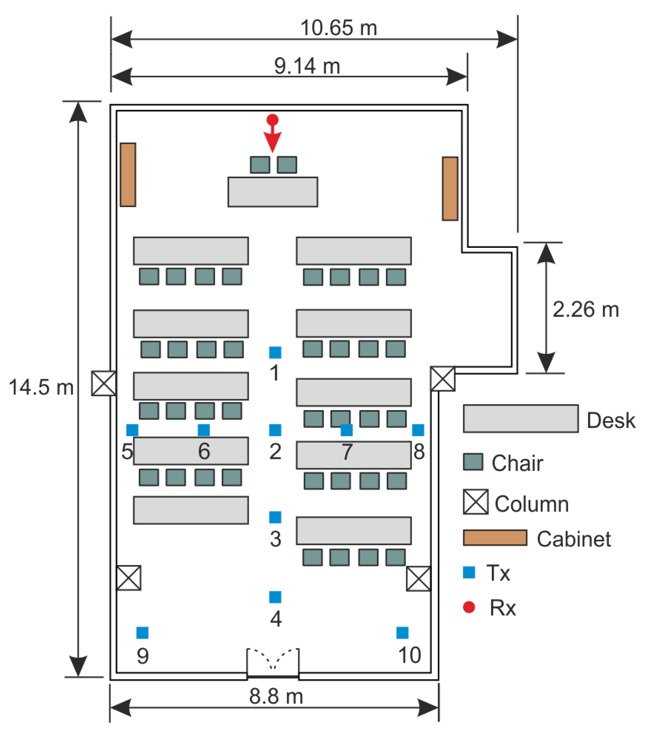
In order to compare both measurements and simulations, and check the agreement between the results achieved, the indoor scenario presented in Figure 2 was considered as a testbed. The room was located in a modern building made of reinforced concrete with indoor ceiling boards, plasterboard panelled walls, metallic doors and a height from the floor to the ceiling board of 2.98 m.
In order to resemble the up-link in a massive MIMO cell for the measurement campaign, the Tx, i.e., an active UT, was placed at 10 different positions and fixed on a Teflon mast at a height of 1.48 m. At the same time, the 2D scanner, i.e., the Rx, was placed close to the rear wall of the room with the centre of the URA at a height of 2 m. As already stated in Section 2.1, and presented in Table 1, for any of the Tx locations considered, the Rx moved on the YZ plane implementing a URA 10 × 10 positions in size. According to the layout presented in Figure 2, the Tx–Rx (or UT–BS) distances lay in the range of 5.8–13.4 m.
For the analysis with the simulator, an electric-geometrical model was generated. Every wall, floor, ceiling, column or piece of furniture was geometrically modelled using a total of 94 flat facets. The electromagnetic properties (relative dielectric constant, electric conductivity, standard deviation of surface roughness and transmission loss) of these facets were chosen from [22] for the different materials: wood for cabinets, chairs and tables and brick or plasterboard for the walls. The authors chose the values recommended by the ITU in [22] because it is a source that can be considered a standard accessible to the scientific community. However, there are other possibilities, among them that of optimising the RT results using heuristic methods, based on a search of electromagnetic values closer to those of the real environment [23].
A grid of 100 × 100 points was considered for the Rx (BS), analysing for each of these points the contribution of the direct ray, up to the seventh reflected ray (R7); diffracted and double diffracted rays and reflected–diffracted and diffracted–reflected rays. The position and polarisation of the antennas were the same as the ones used in the measurements. The radiation pattern and gain of the antennas were synthesised in order to have a model as similar as possible to the real antennas used for the measurements.
3.1.1. Temporal Dispersion
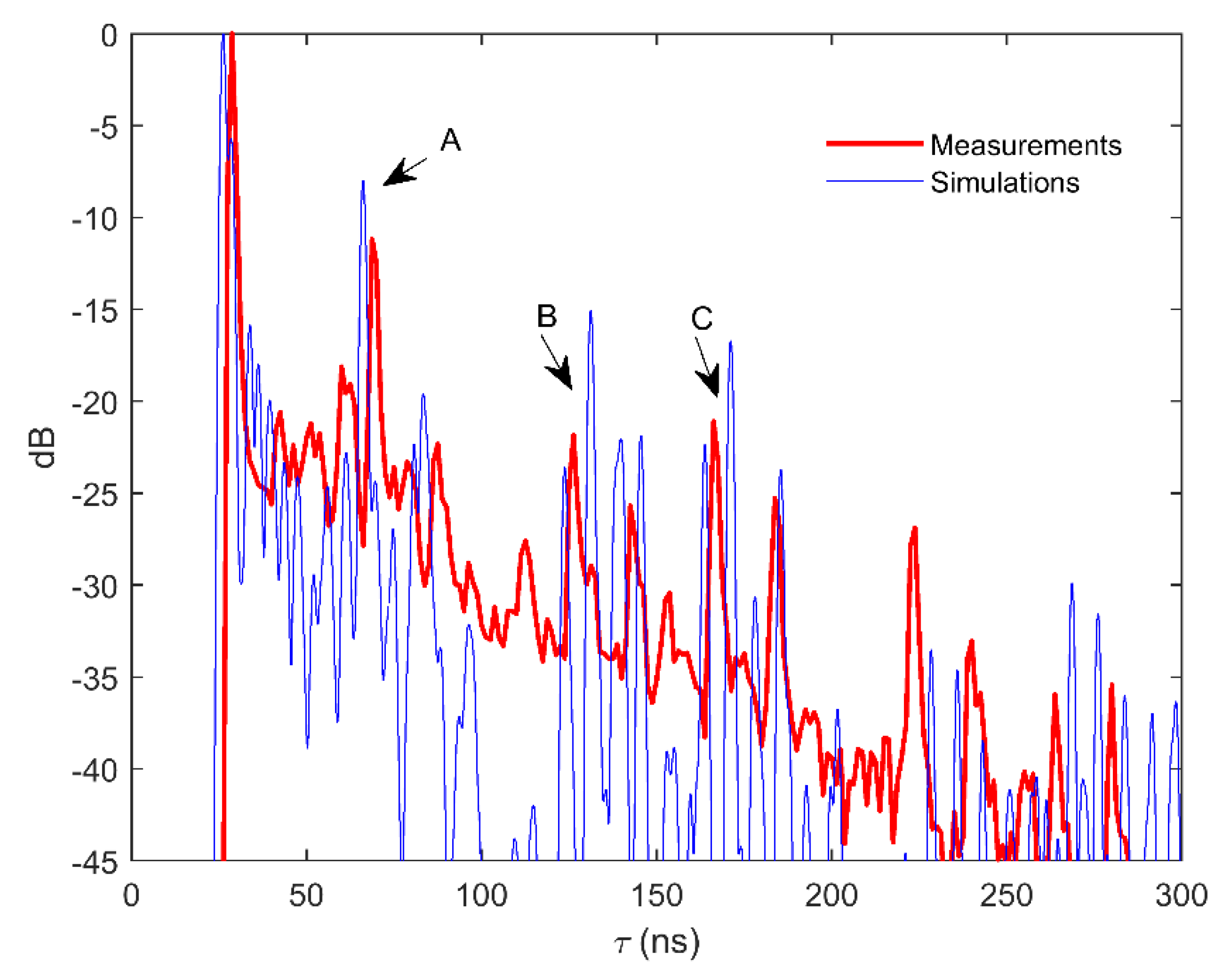
The temporal dispersion of the transmitted signals caused by the radio channel, which is the origin of the frequency selectivity, has a decisive influence on the communications systems performance. As outlined in the previous section, the mean delay and the RMS delay spread can be directly obtained from the PDP. A comparison between measured and simulated PDPs is presented in Figure 3. The PDPs correspond with the mean of the one hundred PDPs obtained for UT#2 (see Figure 2). A good agreement between measurements and simulations can be observed. Due to the relative simplicity of the scenario, it is possible to identify some relevant multipath contributions, denoted in Figure 3 as: A: caused by a very strong first order reflection (R1) on the metallic door of the room and B and C: due to R2 and R3 reflections, respectively, based on the interaction with the metallic door of the room and the concrete back wall.
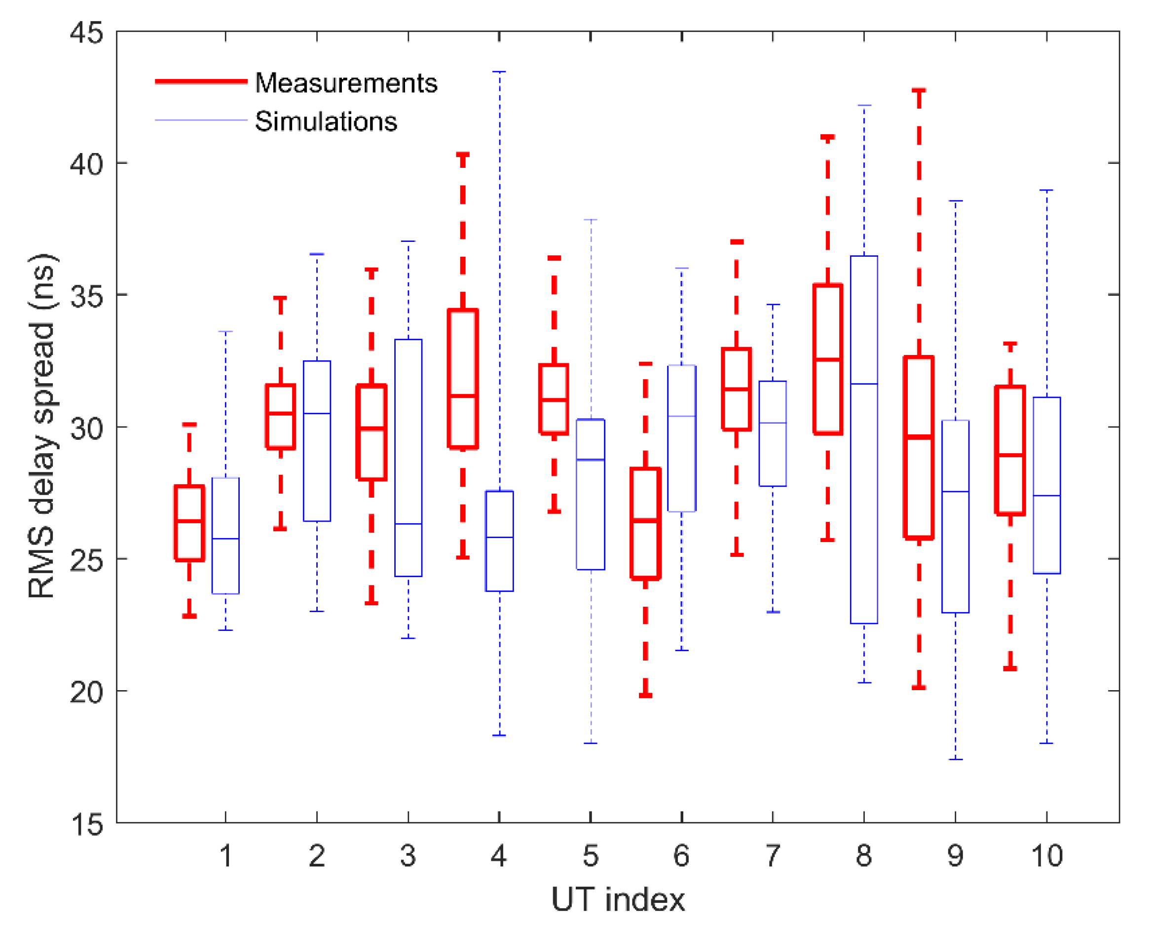
Figure 4 shows the RMS delay spread values obtained for the set of UTs considered, comparing the measurement and simulation results. One hundred RMS delay spread values obtained for each UT along the antenna elements that make up the array were statistically analysed. The top and bottom of each box represent the 25% and 75% percentiles of the samples, respectively, and thus, the distance between both the top and bottom of the box represents the interquartile range. Whiskers were drawn from the ends of the interquartile ranges of the furthest observations. A great dispersion of the RMS delay spread values achieved is observed for most of the UT positions. This variability is caused by the appearance and disappearance of certain multipath components along the elements of the array, in part due to the relatively large size of the array with respect to the propagation environment. The accuracy with which the simulations reproduce the measurements is remarkable.
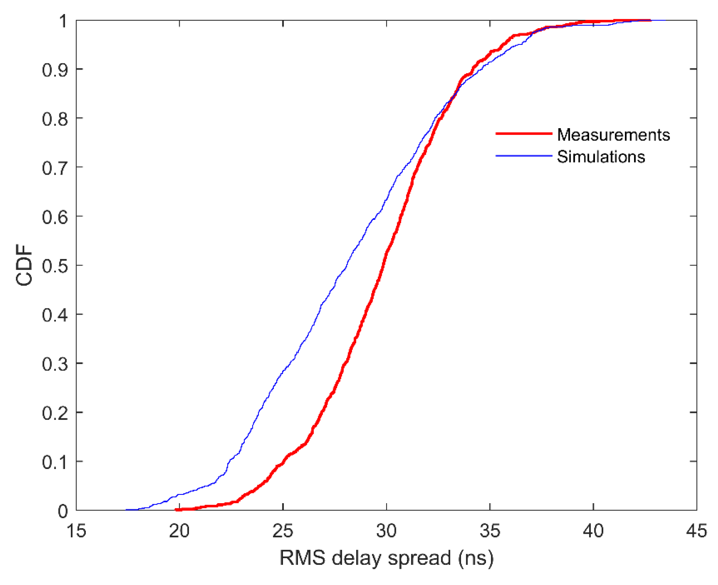
In order to provide a description of the global behaviour of the RMS parameter in the environment under study, its CDF is presented in Figure 5. Once again, the good agreement between measurements and simulations can be observed, especially in the upper tail of the CDF. In this way, the maximum RMS values in the environment, as well as the RMS delay spread τRMS (90%), can be accurately predicted, that is, the value that will only be exceeded in 10% of the channel realisations.
Other results published in the literature show similar values in frequency bands close to 3 and 4 GHz. For instance, in [12], in the same environment (site 1) but using different antennas and a BS location, the RMS delay spread varied from 18 to 35 ns. Furthermore, in [24], values of the RMS delay spread ranging from 5.5 to 15 ns were obtained at 2.4 GHz in LOS conditions for indoor environments, whereas the values in NLOS were higher, ranging from 9 to 23 ns. In the same indoor environment, the value of the RMS delay spread ranged from 8 to 18.0 ns and from 10.6 to 23.6 ns at 4.75 GHz in LOS and NLOS conditions, respectively. In [25], the value of the RMS delay spread oscillated from 22 to 30 ns in LOS conditions at 2.4 GHz. Nevertheless, the values reported in [26] at 3.5 GHz show no appreciable differences between LOS and NLOS conditions, and values from 20 up to 70 ns were derived in indoor environments.
3.1.2. Frequency Selectivity
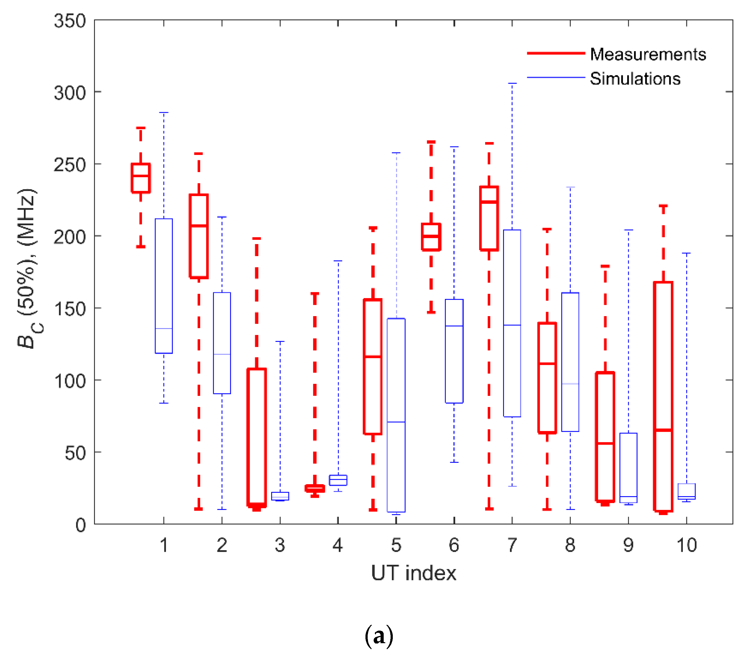
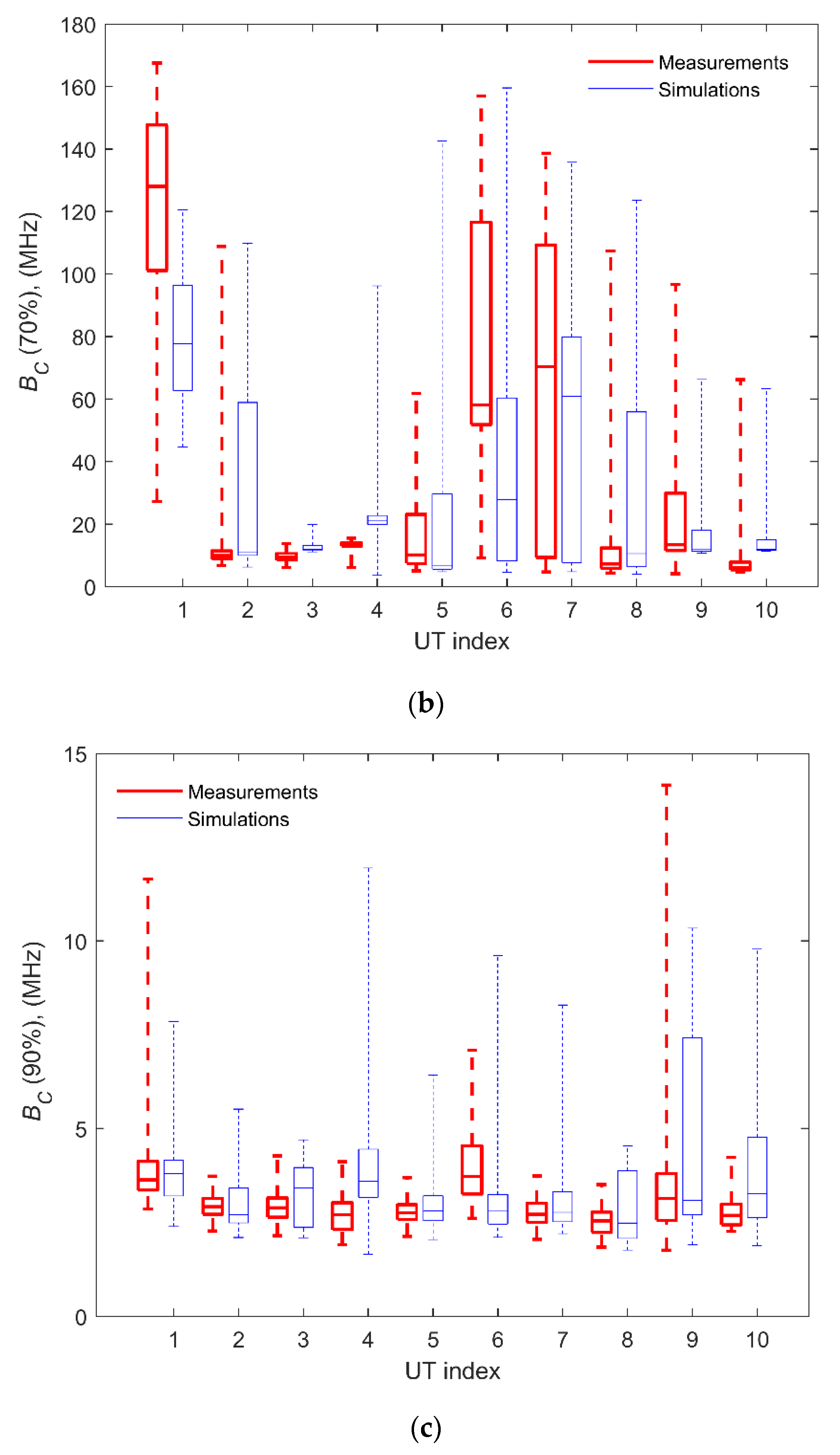
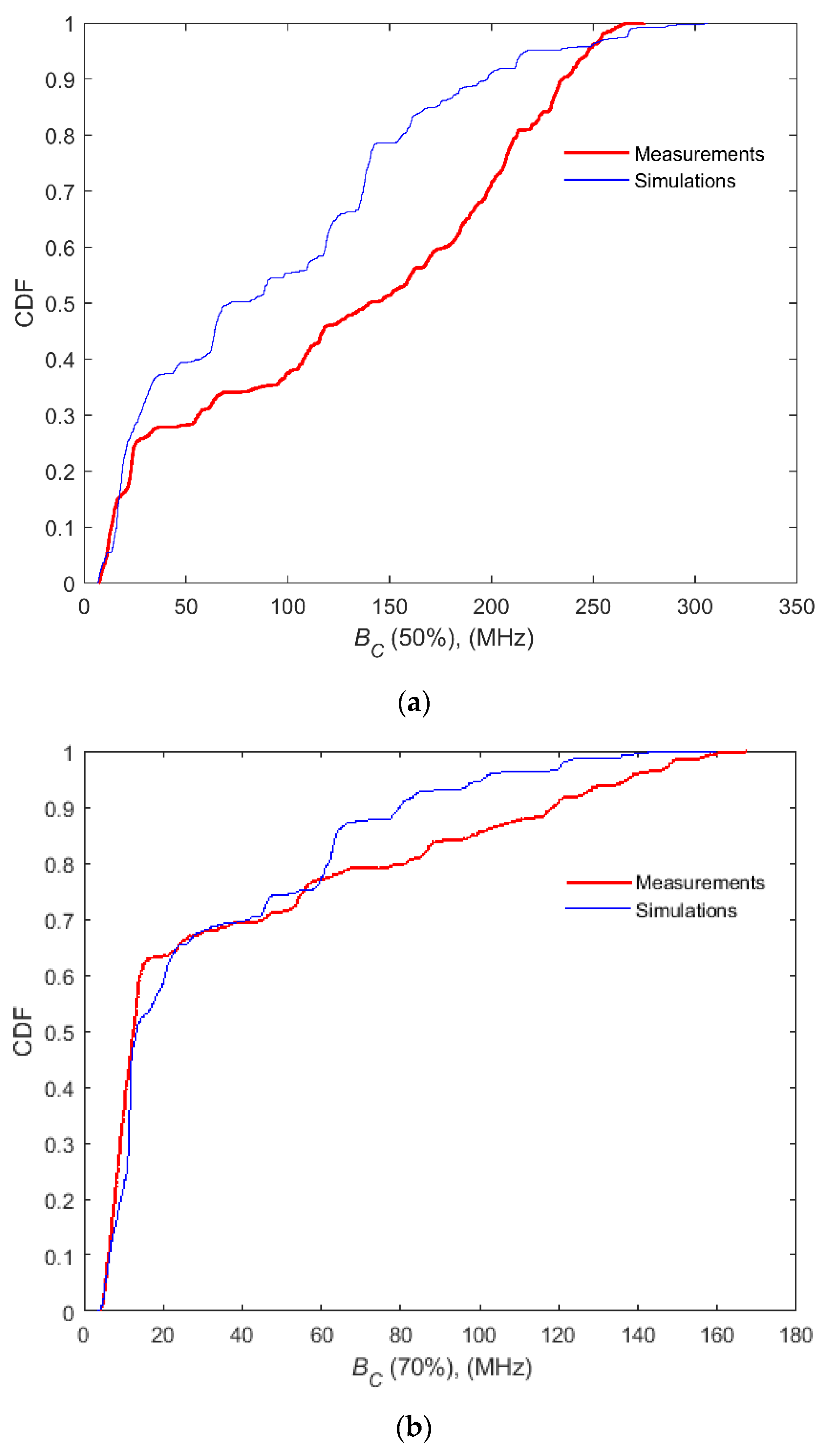
Figure 6 shows the BC values obtained for 50%, 70% and 90% correlation levels. In accordance with the values of the RMS delay spread obtained, a significant dispersion of the BC values is observed for most UTs, and this dispersion decreases as the degree of correlation increases. Again, there is a good agreement between measurements and simulations. The accuracy of the simulations is also evident when analysing the behaviour of the BC for the whole scenario, as shown in Figure 7. In this case, there is a dual behaviour in the CDF of the τRMS, with the lower tails of the CDFs being those that are more similar. In this case, the exact simulation of the lower values of BC are those that acquire the most interest. Table 2 shows the τRMS and BC values of interest, both measured and simulated. A similar range of Bc values, as well as the observed variability throughout the array elements, have been obtained in the measurement campaigns presented in [12,14].
3.1.3. Sum Capacity
From the point of view of the characterisation of a MaMi channel, the sum capacity versus the number of active UTs is a fundamental parameter, which shows the upper limit of the achievable spectral efficiency in a specific environment. RT techniques have been used previously to simulate MIMO channels, most of the time in the context of point-to-point systems, with a low number of antennas at both ends of the link [19,27,28]. The work in [29] presents the validation of an RT simulator in the 60 GHz band for the analysis of beamforming techniques in indoor communications. Furthermore, RT methods are proposed as a real-time prediction tool to assist future beamforming techniques. Regarding the simulation and analysis of properly massive MIMO systems, RT has been proposed in [8,9,10]. An example of application is presented in [8], although the results were not compared with measurements. In [9], RT was applied to simulate a multi-cellular MaMi system in a real and complex urban environment, and the results were compared with simulations based on stochastic i.i.d Rayleigh channels. In [10], an RT method was applied to simulate a MaMi system in an industrial environment in the 3.1–5.3 GHz UWB band, but the results were not compared with measurements.
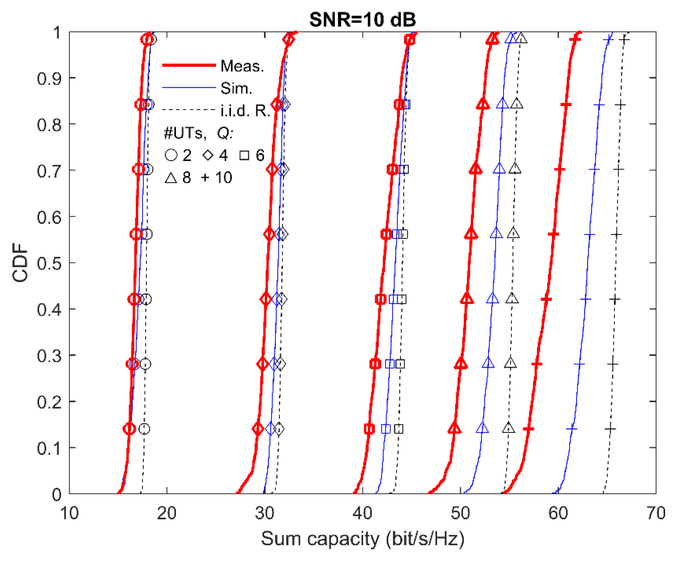
In Figure 8, the CDFs of the sum capacity for different numbers of active UTs, and considering an SNR of 10 dB, are presented for both the measured and simulated channel. The CDFs corresponding with an i.i.d Rayleigh channel are also plotted as a reference. A good agreement between measurements and simulations can be observed, and the error increases as the number of active UTs increases. For the worst case, Q = 10, the error made in predicting the median value of the sum capacity is 3.75 bit/s/Hz, which is 6.3%. It can be observed that the sum capacity of the channel is overestimated for all cases. This fact is most likely due to the differences between the real radiation pattern and gain of the antennas and the simplified ones considered in the simulations [14]. This possible explanation will be analysed in detail in future works.
3.2. MaMi Channel Characterisation in a Large Room
The results reported and discussed in the previous subsection demonstrate the accuracy and usefulness of the simulator, so it can be used itself to analyse the channel performance in other environments without the requirement of carrying out an empirical analysis, of special interest when studying the propagation in large, complex buildings with difficult access.
In this subsection, an assembly hall with a stepped profile, eleven rows of seats and a capacity for more than 200 people, is considered to investigate the main wireless channel parameters using the RT model. The 3D-view of the room is presented in Figure 9a, and it should be noted that the room is located in a modern building made of reinforced concrete, with side walls made of bricks and a mixture of wood and marble for the floor. The electrical properties of these materials were again obtained from [22], and the geometrical model consisted of 693 flat facets.
As depicted in the top view shown in Figure 9b, up to 18 Tx locations, i.e., active UTs, were considered, nine on the left of the main central corridor and the rest on the right side. In order to resemble the BS, the analysis was carried out considering a URA 10 × 10 elements in size, whose centre was 2.2 m from the floor. The transmitter and receiver antennas and coupling mechanisms were the same as those considered in the previous analysis, but the sixth and seventh reflected fields were not considered this time to reduce the simulation time.
With the intention of analysing the results obtained, we compared them with the simulated results already obtained in the calibration environment (see Section 3.1 or Figure 2). For the sake of brevity, we will call the aforementioned calibration environment site 1, and the assembly hall will be site 2.
3.2.1. Temporal Dispersion
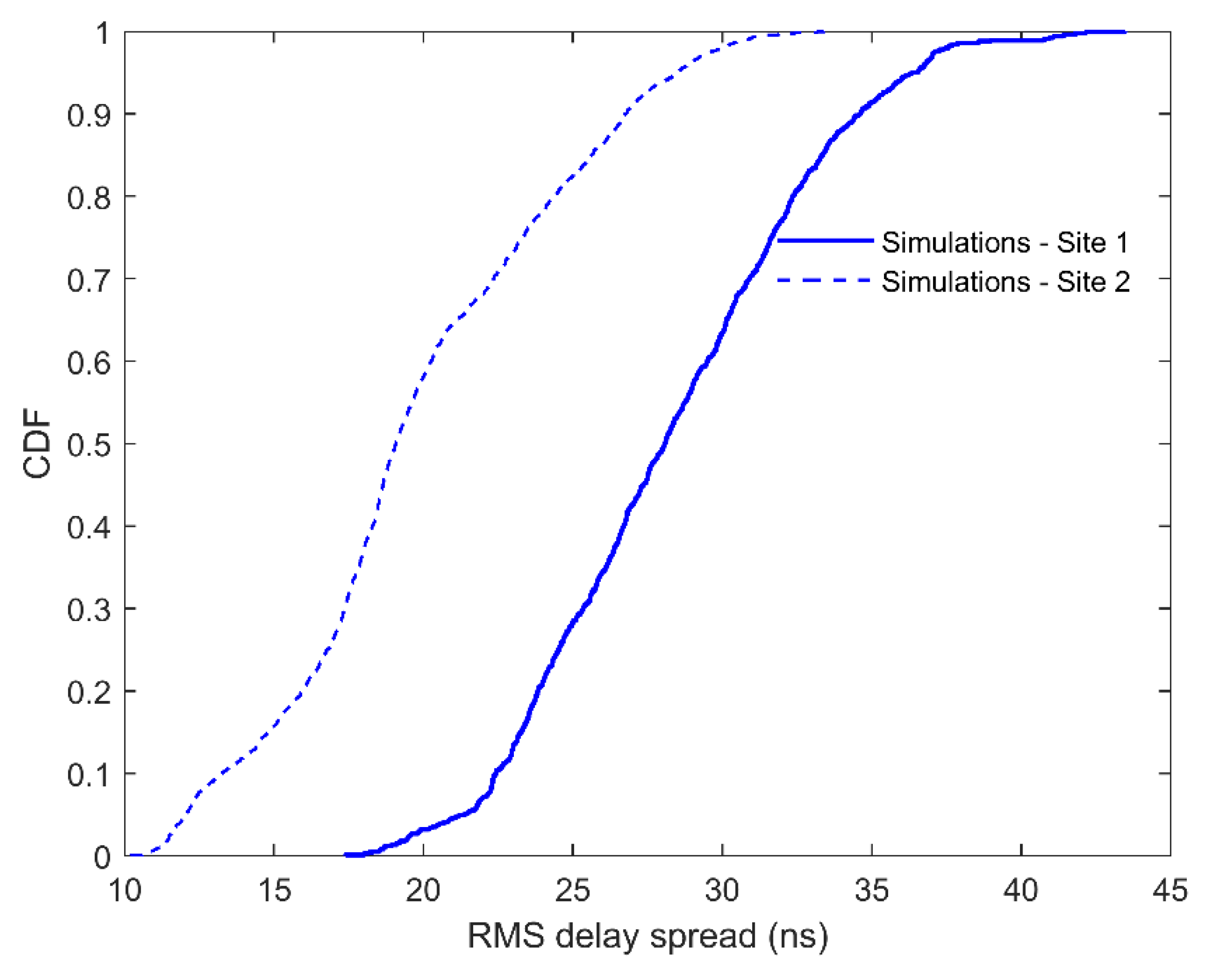
Figure 10 shows a comparison of the CDF of the RMS delay spread obtained with the simulator for both scenarios, sites 1 and 2. The RMS delay spread values show that site 2 is a slightly less dispersive environment than site 1. This is because, while larger, the assembly hall is more furnished, and its stepped floor reduces the possibility of multiple reflections between the ceiling, floor and walls.
3.2.2. Frequency Selectivity
Possibly, the second characteristic of the radio channel that, after the compliance with the favourable propagation condition, most affects the performance of MaMi systems is the coherence bandwidth. This is because the BC, along with the coherence time, determine the length of the so-called coherence block. During this frequency-time block, the channel can be approximated as flat in frequency and time-invariant, and therefore the channel estimate is kept up to date. Thus, the CDFs of the BC for several levels of coherence are important information, which provide a statistical estimate of the values that this parameter may reach in a specific environment.
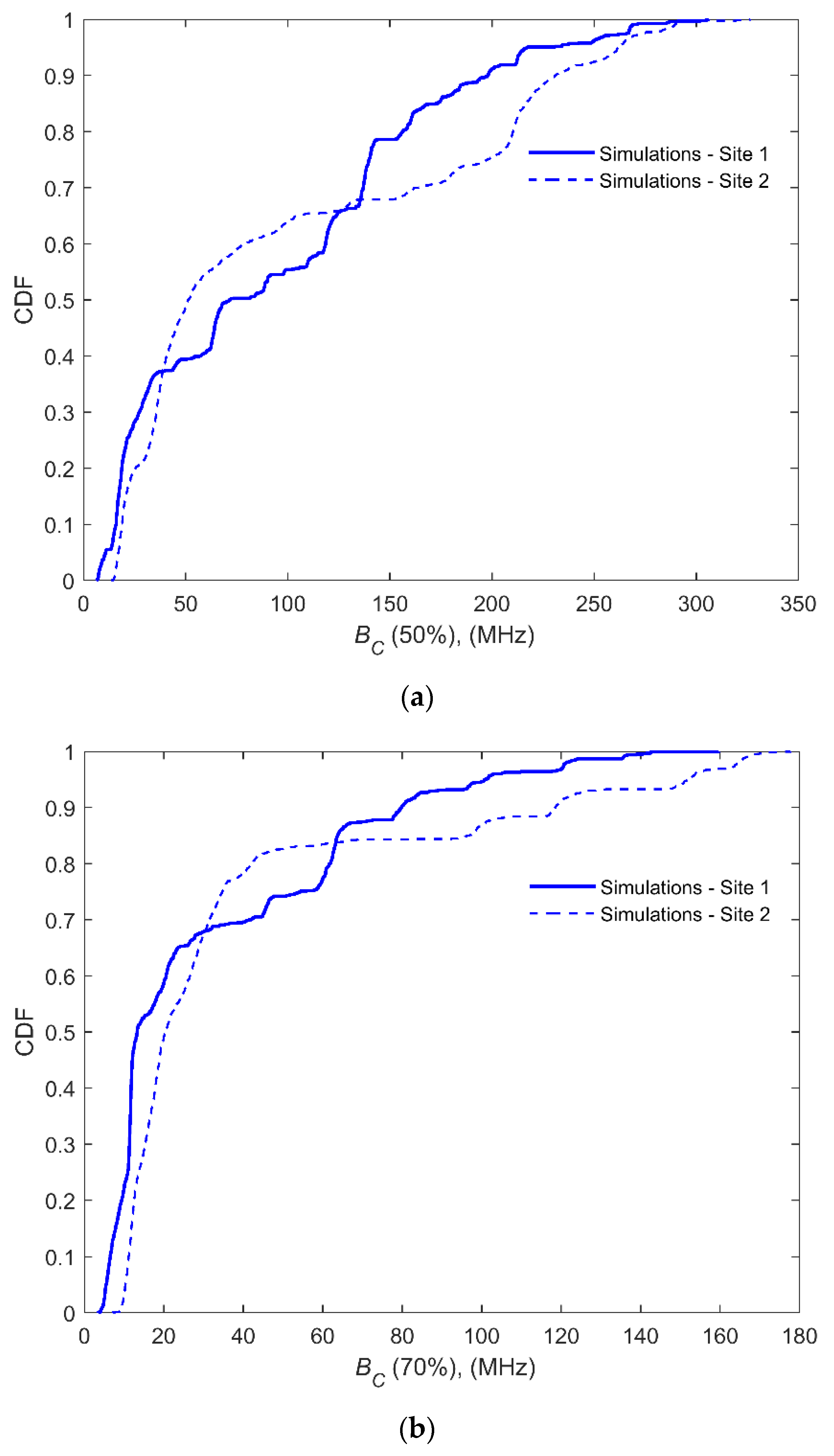
Figure 11 shows a comparison of the CDFs of the coherence bandwidth values obtained with RT for both scenarios, sites 1 and 2, and for different correlation levels: (a) 50%, (b) 70% and (c) 90%. Because of the inverse relationship that exists between the RMS delay spread and BC, it can be seen that the values of the BC obtained in site 1 are, in general, lower than those for site 2. However, there is a convergence in the lower tail of the CDF, which indicates that the most interesting values of BC do not differ too much in the two scenarios. A comparison between them is presented in Table 3.
3.2.3. Sum Capacity
The sum capacity of the channel (in our case, calculated for the up-link), determines the maximum spectral efficiency that can be achieved in a specific cell such as the one analysed.
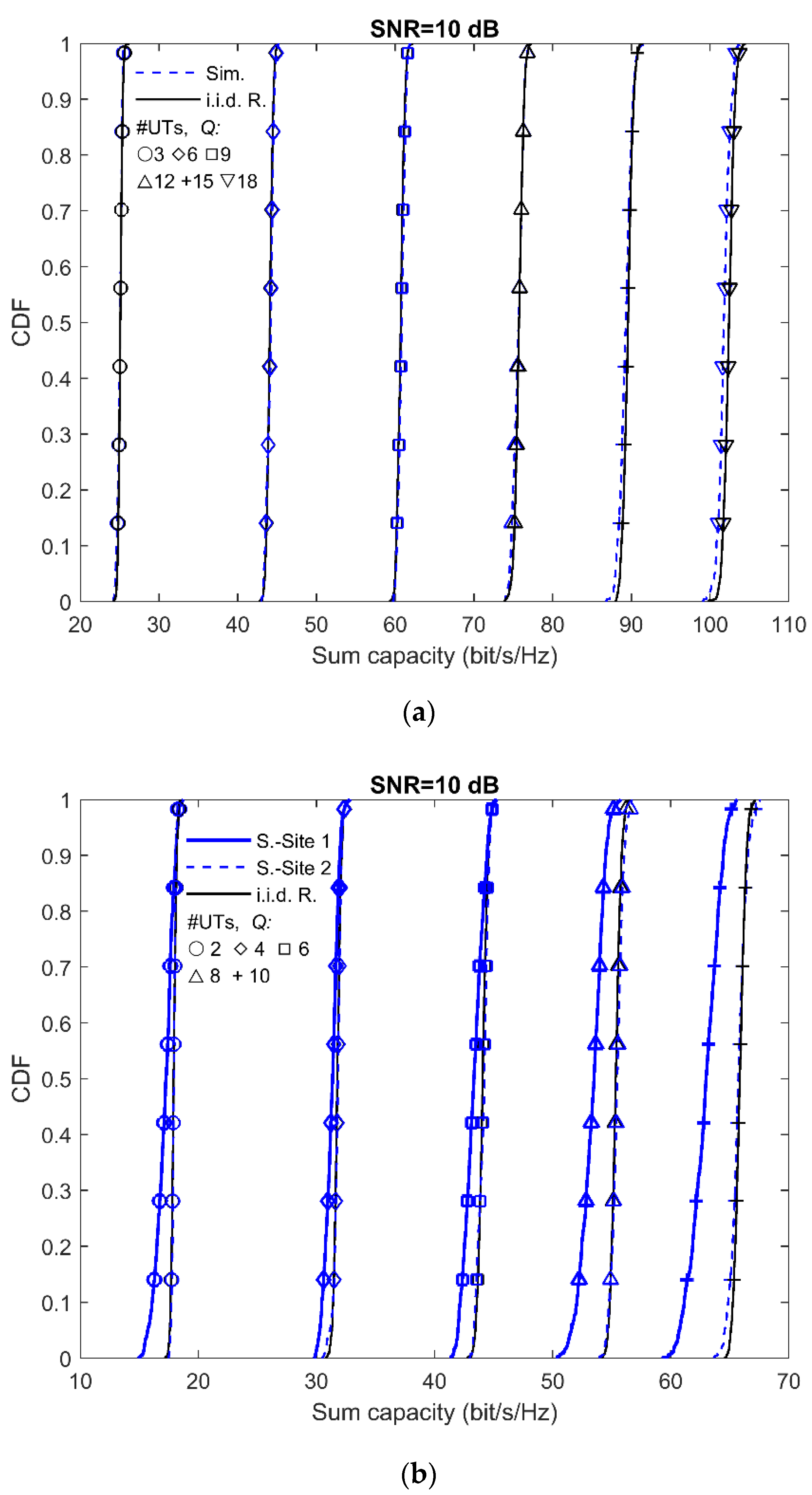
Figure 12a shows CDFs of the sum capacity obtained with RT at the assembly hall considering an SNR of 10 dB. The number of simultaneously active UTs ranges from 3 to 18, and they were randomly chosen. The results were also compared with the values achieved by an i.i.d. Rayleigh channel. The results practically coincide with those of i.i.d Rayleigh channels. This fact indicates that the favourable propagation condition was largely fulfilled, i.e., that the sub-channels established between each UT and the BS were orthogonal to each other. The orthogonality displayed by the sub-channels is due to the richness of scattering in the environment along with the fact that the UTs were distributed in positions and heights that were not very symmetrical.
Figure 12b shows the results achieved for sites 1 and 2 for a number of active UTs ranging from 2 to 10 and randomly chosen. It can be seen how in site 1, the capacity values obtained are lower than in site 2, which is explained by the fact that the environment and the position of the UTs is much more symmetrical in site 1 than in site 2. However, as shown in Section 3.1.3, the capacity results obtained by RT appear slightly overestimated compared to the measurement results.
4. Conclusions
The aim of this research focused on the analysis of the applicability of ray-tracing techniques to model massive MIMO channels. We have presented a case study in order to show the way in which site-specific models based on rigorous RT techniques used in conjunction with limited measurement campaigns can contribute to the development and deployment of systems using the MaMi technique. The case consisted of characterising a large assembly hall with difficult access and measurement restrictions, starting from the measurements and verification of the simulator in another similar but simpler and accessible scenario. The main conclusions are:
The simulated results of the wideband main parameters, i.e., the RMS delay spread and the BC at different correlation levels, were very accurate, making it possible to obtain with low relative error the most influential broadband parameters in the performance of MaMi-TDD-OFDM systems, as the minimum BC values, which determine the size of the coherence block. A great dispersion of the RMS delay spread and BC values along the array elements was observed for most of the UT positions. The accuracy with which the simulations reproduced this variability was appreciable.
Concerning the sum capacity results achieved with the simulator, it can be concluded that these were also accurate. In this case, it could be seen that the capacity was systematically slightly overestimated by the simulator, the relative error of the median capacity being of the order of 6% for the worst case. This fact was most likely due to the differences between the real radiation pattern of the antennas and the simplified ones considered in the simulations, and this possible explanation will be analysed in detail in future works.
If we focus on the comparison of the two environments, it can be seen that site 1 was more time dispersive than site 2, even though site 2 had larger dimensions. This characteristic can be explained by the fact that the assembly hall was more furnished and had a sloping floor, and both characteristics made the appearance of higher order multipath components diminish. Regarding capacity, the hall presented values very close to those associated with an i.i.d. Rayleigh channel, which allowed us to affirm that a great orthogonality between the channels of the different UTs was reached. In this case, the complexity and size of the environment helped in the compliance with the favourable propagation condition. Furthermore, the verification environment was more symmetrical and less furnished, and the UTs were located on a regular basis and placed at the same height. All the aforementioned factors favoured a loss of orthogonality of the sub-channels.
Finally, we can conclude that rigorous RT techniques are valuable engineering tools useful for the analysis, design and deployment of systems based on massive MIMO techniques.
Author Contributions
Conceptualization, L.V. and R.P.T.; methodology, J.R.P. and R.P.T.; software, L.V. and J.R.P.; validation, L.V., J.R.P. and R.P.T.; formal analysis, L.V. and J.R.P.; data curation, J.R.P. and L.V.; supervision, R.P.T.; writing—original draft preparation, L.V., J.R.P. and R.P.T. All authors have read and agreed to the published version of the manuscript.
Funding
This work has been supported by the Spanish Ministry of the Economy, Industry and Competitiveness (TEC2017-86779-C2-1-R).
Conflicts of Interest
The authors declare no conflict of interest.
References
- Ghazal, A.; Yuan, Y.; Wang, C.; Zhang, Y.; Yao, Q.; Zhou, H.; Duan, W. A non-stationary IMT-advanced MIMO channel model for high-mobility wireless communication systems. IEEE Trans. Wirel. Commun. 2017, 16, 2057–2068. [Google Scholar] [CrossRef] [Green Version]
- Jaeckel, S.; Raschkowski, L.; Börner, K.; Thiele, L. QuaDRiGa: A 3-D multi-cell channel model with time evolution for enabling virtual field trials. IEEE Trans. Antennas Propag. 2014, 62, 3242–3256. [Google Scholar] [CrossRef]
- Flordelis, J.; Li, X.; Edfors, O.; Tufvesson, F. Massive MIMO Extensions to the COST 2100 Channel Model: Modeling and Validation. IEEE Trans. Wirel. Commun. 2020, 19, 380–394. [Google Scholar] [CrossRef] [Green Version]
- Schuster, W.; Luebbers, R.J. Comparison of GTD and FDTD predictions for UHF radio wave propagation in a simple outdoor urban environment. In Proceedings of the IEEE Antennas and Propagation Society International Symposium, Montreal, QC, Canada, 13–18 July 1997; Volume 3, pp. 2022–2025. [Google Scholar] [CrossRef]
- Kouyoumjian, R.G.; Pathak, P.H. A uniform geometrical theory of diffraction for an edge in a perfectly conducting surface. Proc. IEEE 1974, 62, 1448–1461. [Google Scholar] [CrossRef] [Green Version]
- Luebbers, R.J. Finite conductivity uniform GTD versus knife edge diffraction in prediction of propagation path loss. IEEE Trans. Antennas Propag. 1984, AP-32, 70–76. [Google Scholar] [CrossRef]
- McNamara, D.A.; Pistorius, C.W.I.; Malherbe, J.A.G. Introduction to the Uniform Geometrical Theory of Diffraction; Artech House: Norwood, MA, USA, 1990. [Google Scholar]
- He, D.; Ai, B.; Guan, K.; Wang, L.; Zhong, Z.; Kürner, T. The design and applications of high-performance ray-tracing simulation platform for 5G and beyond wireless communications: A tutorial. IEEE Commum. Surv. Tutor. 2019, 21, 10–27. [Google Scholar] [CrossRef]
- Aslam, M.Z.; Corre, Y.; Björnson, E.; Larsson, E.G. Large-scale massive MIMO network evaluation using ray-based deterministic simulations. In Proceedings of the IEEE 29th Annual International Symposium on Personal, Indoor, and Mobile Radio Communications, Bologna, Italy, 9–12 September 2018. [Google Scholar] [CrossRef] [Green Version]
- Fathy, A.; Newagy, F.; Anis, W.R. Performance evaluation of UWB massive MIMO channels with favorable propagation features. IEEE Access 2019, 7, 147010–147020. [Google Scholar] [CrossRef]
- Moreno, J.; Domingo, M.; Valle, L.; Pérez, J.R.; Torres, R.P.; Basterrechea, J. Design of indoor WLANs: Combination of a ray-tracing tool with the BPSO method. IEEE Antennas Propag. Mag. 2015, 57, 22–33. [Google Scholar] [CrossRef] [Green Version]
- Pérez, J.R.; Torres, R.P.; Rubio, L.; Basterrechea, J.; Domingo, M.; Rodrigo, V.M.; Reig, J. Empirical characterization of the indoor radio channel for array antenna systems in the 3 to 4 GHz frequency band. IEEE Access 2019, 7, 94725–94736. [Google Scholar] [CrossRef]
- Torres, R.P.; Pérez, J.R.; Basterrechea, J.; Domingo, M.; Valle, L.; González, J.; Rubio, L.; Rodrigo, V.M.; Reig, J. Empirical characterisation of the indoor multi-user MIMO channel in the 3.5 GHz band. IET Microw. Antennas Propag. 2019, 13, 2386–2390. [Google Scholar] [CrossRef] [Green Version]
- Pérez, J.R.; Torres, R.P. On the impact of the radiation Pattern of the antenna element on MU-MIMO indoor channels. IEEE Access 2020, 8, 25459–25467. [Google Scholar] [CrossRef]
- Torres, R.P.; Valle, L.; Domingo, M.; Loredo, S.; Diez, M.C. Cindoor: An engineering tool for planning and design of wireless systems in enclosed spaces. IEEE Antennas Propag. Mag. 1999, 41, 11–22. [Google Scholar] [CrossRef]
- Fernández, Ó.; Valle, L.; Domingo, M.; Torres, R.P.; Rays, F. Accurate ray-tracing for planning and design. IEEE Veh. Technol. Mag. 2008, 3, 18–27. [Google Scholar] [CrossRef]
- Loredo, S.; Valle, L.; Torres, R.P. Accuracy analysis of GO/UTD radio-channel modeling in indoor scenarios at 1.8 and 2.5 GHz. IEEE Antennas Propag. Mag. 2001, 43, 37–51. [Google Scholar] [CrossRef]
- Torres, R.P.; Loredo, S.; Valle, L.; Domingo, M. An accurate and efficient method based on ray-tracing for the prediction of local flat-fading statistics in picocell radio channels. IEEE J. Sel. Areas Commun. 2001, 18, 170–178. [Google Scholar] [CrossRef]
- Loredo, S.; Rodríguez-Alonso, A.; Torres, R.P. Indoor MIMO channel modeling by rigorious GO/UTD-based ray tracing. IEEE Trans. Veh. Technol. 2008, 57, 680–692. [Google Scholar] [CrossRef]
- Parsons, J.D. Wideband Channel Characterization. The Mobile Radio Propagation Channel, 2nd ed.; John Wiley & Sons: Chichester, UK, 2000. [Google Scholar]
- Gao, X.; Edfors, O.; Rusek, F.; Tufvesson, F. Massive MIMO performance evaluation based on measured propagation data. IEEE Trans. Wirel. Commun. 2015, 14, 3899–3911. [Google Scholar] [CrossRef] [Green Version]
- Effects of Building Materials and Structures on Radiowave Propagation above about 100 MHz. Recommendation ITU-R P.2040-1. Available online: https://www.itu.int/dms_pubrec/itu-r/rec/p/R-REC-P.2040-1-201507-I!!PDF-E.pdf (accessed on 3 August 2020).
- Matschek, R. A geometrical optics and uniform theory of diffraction based ray tracing optimisation by a genetic algorithm. C. R. Phys. 2005, 6, 595–603. [Google Scholar] [CrossRef]
- Janssen, G.; Patrick Stigter, P.; Prasad, R. Wideband indoor channel measurements and BER analysis of frequency selective multipath channels at 2.4, 4.75, and 11.5 GHz. IEEE Trans. Commun. 1996, 44, 1272–1288. [Google Scholar] [CrossRef]
- Zepernick, H.J.; Wysocki, T.A. Multipath channel parameters for the indoor radio at 2.4 GHz ISM band. In Proceedings of the IEEE 49th Vehicle Technology Conference, Houston, TX, USA, 16–20 May 1999; pp. 190–193. [Google Scholar] [CrossRef]
- Huang, F.; Tian, L.; Zheng, Y.; Zhang, J. Propagation characteristics of indoor radio channel from 3.5 GHz to 28 GHz. In Proceedings of the IEEE 84th Vehicular Technology Conference (VTC-Fall), Montréal, QC, Canada, 18–21 September 2016; pp. 1–5. [Google Scholar] [CrossRef]
- Kaya, A.O.; Trappe, W.; Greenstein, L.J.; Chizhik, D. Predicting MIMO performance in urban microcells using ray tracing to characterize the channel. IEEE Trans. Wirel. Commun. 2012, 11, 2402–2411. [Google Scholar] [CrossRef]
- Yang, Y.; Mellios, E.; Beach, M.; Hilton, G. Evaluation of three-element MIMO access points based on measurements and ray tracing models. In Proceedings of the IEEE 26th Annual International Symposium on Personal, Indoor, and Mobile Radio Communications (PIMRC), Hong Kong, China, 30 August–2 September 2015; pp. 419–424. [Google Scholar] [CrossRef]
- Degli-Esposti, V.; Fuschini, F.; Vitucci, E.M.; Barbiroli, M.; Zoli, M.; Tian, L.; Yin, X.; Dupleich, D.; Müller, R.; Schneider, C.; et al. Ray-tracing-based mm-wave beamforming assessment. IEEE Access 2014, 2, 1314–1325. [Google Scholar] [CrossRef]
Figure 1.
Schematic of the measurement setup. (a) Detail of the complete measurement system. (b) Block diagram of the channel sounding system.
Figure 1.
Schematic of the measurement setup. (a) Detail of the complete measurement system. (b) Block diagram of the channel sounding system.


Figure 2.
Top view of the reference environment used to analyse the agreement between measurements and simulations.
Figure 2.
Top view of the reference environment used to analyse the agreement between measurements and simulations.

Figure 3.
Example of the power delay profile (PDP) achieved for UT#2, identifying some relevant multipath contributions. A: strong first order reflection, B: second order reflection, and C: third order reflection.
Figure 3.
Example of the power delay profile (PDP) achieved for UT#2, identifying some relevant multipath contributions. A: strong first order reflection, B: second order reflection, and C: third order reflection.

Figure 4.
RMS delay spread values for the set of active user terminals (UTs) considered.

Figure 5.
CDF of the RMS delay spread for the whole scenario.

Figure 6.
Coherence bandwidth values for the set of UTs considered and for different correlation levels: (a) 50%, (b) 70% and (c) 90%.
Figure 6.
Coherence bandwidth values for the set of UTs considered and for different correlation levels: (a) 50%, (b) 70% and (c) 90%.


Figure 7.
CDF of the coherence bandwidth values for the whole scenario and for different correlation levels: (a) 50%, (b) 70% and (c) 90%.
Figure 7.
CDF of the coherence bandwidth values for the whole scenario and for different correlation levels: (a) 50%, (b) 70% and (c) 90%.


Figure 8.
CDF of the sum capacity for a different number of active UTs, considering an SNR of 10 dB.
Figure 8.
CDF of the sum capacity for a different number of active UTs, considering an SNR of 10 dB.

Figure 9.
Assembly hall. (a) 3D view. (b) Plan view showing the relative position of the receiver antenna (Rx) and the 18 simulated transmitter antennas (Txs).
Figure 9.
Assembly hall. (a) 3D view. (b) Plan view showing the relative position of the receiver antenna (Rx) and the 18 simulated transmitter antennas (Txs).

Figure 10.
Comparison of the CDF of the RMS delay spread obtained with ray-tracing (RT) for both scenarios, sites 1 and 2.
Figure 10.
Comparison of the CDF of the RMS delay spread obtained with ray-tracing (RT) for both scenarios, sites 1 and 2.

Figure 11.
Comparison of the CDF of the coherence bandwidth values obtained with RT for both scenarios, sites 1 and 2, and for different correlation levels: (a) 50%, (b) 70% and (c) 90%.
Figure 11.
Comparison of the CDF of the coherence bandwidth values obtained with RT for both scenarios, sites 1 and 2, and for different correlation levels: (a) 50%, (b) 70% and (c) 90%.


Figure 12.
CDF of the sum capacity obtained with the simulator at the assembly hall considering an SNR of 10 dB. The results are also compared with the values achieved by an i.i.d. Rayleigh channel: (a) results achieved for a number of active UTs ranging from 3 to 18 and randomly chosen, and (b) comparative results achieved for sites 1 and 2 for a number of active UTs ranging from 2 to 10 and randomly chosen.


Table 1.
Summary of the most representative parameters considered for the measurement campaign.
| Frequency range (GHz) | 3.2–4.0 |
| Frequency tones, Nf | 641 |
| Frequency resolution, Δf (MHz) | 1.25 |
| VNA power at Port 1 (dBm) | 9 |
| VNA IF bandwidth (kHz) | 3 |
| Signal to noise ratio (SNR) observed at any Tx position (dB) | >45 |
| URA inter-element separation Δy = Δz (mm/λ) | 50/0.53 at 3.2 GHz |
| URA, total scanning area (m2) | 0.2025 |
Table 2.
Comparison between representative statistical values of τRMS (ns) and Bc (MHz), measured and simulated.
Table 2.
Comparison between representative statistical values of τRMS (ns) and Bc (MHz), measured and simulated.
| Analysis | τRMS (90%) | Bc0.5 (10%) | Bc0.7 (10%) | Bc0.9 (10%) |
|---|---|---|---|---|
| Measurements | 34.2 | 13.2 | 6.2 | 2.3 |
| Simulations | 34.6 | 15.9 | 6.5 | 2.5 |
| Error (%) | 1.7 | 17.0 | 4.6 | 8.0 |
Table 3.
Representative statistical values of τRMS (ns) and Bc (MHz) in site 1 and site 2.
| Situation | τRMS (90%) | Bc0.5 (10%) | Bc0.7 (10%) | Bc0.9 (10%) |
|---|---|---|---|---|
| Site 1 | 35.0 | 16.0 | 6.5 | 2.3 |
| Site 2 | 27.0 | 18.8 | 11.2 | 3.2 |
© 2020 by the authors. Licensee MDPI, Basel, Switzerland. This article is an open access article distributed under the terms and conditions of the Creative Commons Attribution (CC BY) license (http://creativecommons.org/licenses/by/4.0/).
Share and Cite
MDPI and ACS Style
Valle, L.; Pérez, J.R.; Torres, R.P. Characterisation of Indoor Massive MIMO Channels Using Ray-Tracing: A Case Study in the 3.2–4.0 GHz 5G Band. Electronics 2020, 9, 1250. https://doi.org/10.3390/electronics9081250
AMA Style
Valle L, Pérez JR, Torres RP. Characterisation of Indoor Massive MIMO Channels Using Ray-Tracing: A Case Study in the 3.2–4.0 GHz 5G Band. Electronics. 2020; 9(8):1250. https://doi.org/10.3390/electronics9081250
Chicago/Turabian StyleValle, Luis, Jesús R. Pérez, and Rafael P. Torres. 2020. "Characterisation of Indoor Massive MIMO Channels Using Ray-Tracing: A Case Study in the 3.2–4.0 GHz 5G Band" Electronics 9, no. 8: 1250. https://doi.org/10.3390/electronics9081250
Note that from the first issue of 2016, this journal uses article numbers instead of page numbers. See further details here.