


1. Introduction
The Antarctic ice sheet is the largest volume of solid water on Earth, and the melting of this ice sheet under a warming climate will cause a significant increase in the global sea level (Tang and others, Reference Tang, Sun, Li, Cui and Li2009; Rignot and others, Reference Rignot, Velicogna, van den Broeke, Monaghan and Lenaerts2011). The mass input on the surface of the Antarctic and Greenland ice sheets can be expressed by surface mass balance (SMB), which is the most important parameter when studying the state of ice sheets under different climatic conditions (Verfaillie and others, Reference Verfaillie2012; Lenaerts and others, Reference Lenaerts, Medley, van den Broeke and Wouters2019). SMB is influenced by slope, elevation, wind direction, wind speed and air temperature (Lenaerts and others, Reference Lenaerts, Medley, van den Broeke and Wouters2019). Although the SMB gradually decreases with distance inland from the coast, the SMB varies over several spatial scales, ranging from a few meters to hundreds of kilometers (Ding and others, Reference Ding2011).
Observations of SMB in Antarctica are mainly obtained through on-site measurements and can be used to interpolate remote-sensing data. There are a variety of methods available for on-site ground observations, such as stakes in farms and lines, snow pits, snow micro-pens and firn/ice cores (e.g. Eisen and others, Reference Eisen2008; Kameda and others, Reference Kameda, Motoyama, Fujita and Takahashi2008; Ding and others, Reference Ding2011; Shepherd and others, Reference Shepherd2012; Proksch and others, Reference Proksch, Löwe and Schneebeli2015). However, these methods provide SMB data at a low spatial resolution. For example, the stake data resolution of Ding and others (Reference Ding2011) is 15 km, and the measurements span only 20–30 years. The shortness of the studied time periods cannot be used to directly understand the characteristics of Antarctic SMB changes over century timescales. Ground-penetrating radar (GPR) has the advantage of providing continuous measurements over the ice sheet over larger distances than stakes and ice cores. When combined with other measurements, GPR allows the estimation of past SMB rates (e.g. Verfaillie and others, Reference Verfaillie2012; Meur and others, Reference Meur2018).
The Chinese National Antarctic Research Expedition (CHINARE) has conducted several traverses from Zhongshan station to Dome A, collecting repeat observations along this transect (Mayewski and others, Reference Mayewski2005; Cui and others, Reference Cui, Wang, Sun, Tang and Guo2017). For these regular surveys, CHINARE uses a radar with a central frequency of 179 MHz to measure the ice sheet, allowing the characterization of the subglacial topography along the traverse (Cui and others, Reference Cui2010). However, the frequency used implies that the internal reflecting horizons (IRHs) within several hundred meters at the top of the shallow ice sheet cannot be resolved. Therefore, in the summer of 2015/16, CHINARE used a frequency-modulated continuous wave (FMCW) radar to survey the same transect.
The purpose of this study is to reconstruct the average SMB from Zhongshan station to Dome A over the past few hundred years using high-resolution FMCW radar data. We first described the radar acquisition and processing. Based on the different ice surface characteristics along the traverse route (e.g. slope, meteorology), four distinct regions of the transect were identified for SMB analysis (Fig. 1). We traced IRHs in each transect section, dated them using available age and density information from ice cores collected along the traverse route between ad 1998 and ad 2005, and quantified uncertainties based on the combined radar and ice core measurement, resulting in estimated SMB rates. Finally, we discuss the temporal and spatial variability in the SMB rate in these four distinct transect regions and compare them to independently observed and modeled SMB data.

Fig. 1. Map of the radar traverse route from Zhongshan station to Dome A shown by a blue line. The four distinct transect regions discussed in this study (zone 1, 49–195 km; zone 2, 780–892 km; zone 3, 1080–1157 km; and zone 4, 1157–1236 km from the coast) are highlighted in yellow, green, dark red and magenta, respectively. Orange dots indicate the locations of the ice cores used in our study (LGB69, DT263, DT401 and DA2005), and black triangles indicate the Zhongshan (ZHS) station, Taishan (TAS) station and Dome A.
2. Data
2.1. Radar
FMCW radar, as a remote-sensing technology, has previously proven to be useful in snow research (e.g. Marshall and Koh, Reference Marshall and Koh2008), such as for snow stratigraphy measurement (e.g. Ellerbruch and Boyne, Reference Ellerbruch and Boyne1980; Koh and others, Reference Koh, Lever, Arcone, Marshall and Ray2010), identification of snow features (e.g. Koh and others, Reference Koh, Yankielun and Baptista1996; Yankielun and others, Reference Yankielun, Rosenthal and Davis2004; Marshall and others, Reference Marshall, Schneebeli and Koh2007), avalanche study (e.g. Gubler and Hiller, Reference Gubler and Hiller1984), drainage structure detection in ice (e.g. Arcone and Yankielun, Reference Arcone and Yankielun2000) and object detection in the snow (e.g. Yamaguchi and others, Reference Yamaguchi, Mitsumoto, Sengoku and Abe1992). This radar architecture has a higher resolution than a conventional pulsed radar, but the measurement range is smaller, so these two radar types can be combined to exploit each system's advantages (Uribe and others, Reference Uribe, Zamora, Gacitúa, Rivera and Ulloa2014).
FMCW radar data were obtained during the 32nd CHINARE traverse (15–30 December 2015). CHINARE traveled mostly along 77°E longitude from Zhongshan station to Dome A and passed by Taishan station. The radar's control unit was set in the cabin of a Pisten Bully 300, and the antennas were placed parallel to each other at the top of the left side of the cabin. Because a metal rod would interfere with the signal, two rigid bamboo poles were used to fix the antennas. Both the transmitter and the receiver antenna were eight-element Vivaldi antenna arrays, which significantly narrowed the beamwidth. The half-power beamwidth of the antenna array was ~15° in the E-plane (across track) and ~60° in the H-plane (along track). Therefore, the antennas were installed 1.5 m from the vehicle on a nonmetal frame and 2 m above the ice surface, and the radar echo from the vehicle can be ignored. The vehicle moved at a constant speed of 14 km h−1, and the transmitter and receiver operated continuously. A GPS antenna was mounted on the roof for geolocation and moved at the same speed.
In this radar system, the transmitting antenna produces an electromagnetic wave with a frequency of 0.5–2 GHz and a variation period of 4 ms, and the wavefront propagates downward. As the depth increases, the intensity of the reflected signal changes due to variations in the complex dielectric permittivity with increasing depth. The real part of the complex dielectric permittivity is mainly affected by density changes, whereas the imaginary part is mainly affected by electrical conductivity and dielectric anisotropy (Kovacs and others, Reference Kovacs, Holladay and Bergeron1995; Eisen and others, Reference Eisen2008). For our FMCW radar data, density, which increases with depth in the firn column until it stabilizes near 830 kg m−3 (Eisen and others, Reference Eisen2008), has the strongest influence on the complex dielectric constant (Kanagaratnam and others, Reference Kanagaratnam, Gogineni, Gundestrup and Larsen2001). We analyze the density characteristics in more detail in Section 3.1.
The variations in the complex dielectric permittivity with depth are laterally consistent, which creates continuous reflections called IRHs (Verfaillie and others, Reference Verfaillie2012). A radar echogram typically shows multiple IRHs stacked vertically, presenting a clear layered structure. IRHs from our traverse shown in Figure 2a are spatially continuous, and the formation time of a layer is considered isochronous (Eisen and others, Reference Eisen2008). Due to the influences of the surface slope, elevation, wind direction, wind speed and other factors, SMB variability will impact the depth of the same IRH along the transect (highlighted for three IRHs in Fig. 2b). Therefore, SMB can be reconstructed from IRH depths. The average thickness of the ice sheet from Zhongshan station to Dome A is 2037 m (Cui and others, Reference Cui2010), while the FMCW radar only provides IRH within ~100 m from the surface, so finite strain can be ignored (Waddington and others, Reference Waddington, Neumann, Koutnik, Marshall and Morse2007), and the SMB can be calculated directly from the age and depth of the IRH and the density of the ice core.

Fig. 2. FMCW radar profiles and interpretation. (a) Part of the radar profile and IRHs in zone 1 (138–191 km from the coast). (b) Three IRHs randomly extracted from (a). (c) IRH folds and discontinuities at the end of zone 1 (192–199 km from the coast). (d) Concave and convex patterns in the IRHs at the end of zone 2 (753–783 km from the coast).
The radar profiles collected between Zhongshan station and Dome A (with a total length of 1236 km) were processed. In practice, when tracking an IRH over a range of more than 100 km, lateral discontinuities in the IRH are often found (Fig. 2), and it is difficult to trace a single IRH. In some locations, a complex structure in the ice sheet or a technical issue such as a break in the field recording can result in the loss of lateral continuity of the IRH. Figure 2c shows an example of a fold and discontinuity affecting multiple IRHs and Figure 2d displays strongly sloping IRHs. Such IRH geometries may be due to local ice flow causing overlap from different IRHs and snow mixing to cause radar reflection distortion (Arcone and Jacobel, Reference Arcone and Jacobel2010a, Reference Arcone and Jacobel2010b; Dahl-Jensen and others, Reference Dahl-Jensen2013). Additionally, the melting of snow at the surface will also lead to the disappearance of IRH (e.g. Arcone and Jacobel, Reference Arcone and Jacobel2010b; Jacobel and Hodge, Reference Jacobel and Hodge1995).
Based on the characteristics of topography, SMB, IRH continuity, etc., four distinct transect regions (Fig. 1) were identified. Due to the limitation of radar detection depth and IRH discontinuity, IRHs in the same year cannot be extracted across these regions at the same time. Instead, three random ages of IRHs in each region were manually selected and tracked (e.g. Fig. 2b) and TWT was converted to depth (as described in Appendix A) for which we calculate the SMB over the past few hundred years. We define these four zones as follows:
-
Zone 1 is located 49–195 km from the coast, with steep and gradually decreasing slopes along the traverse (slopes range from 6.47 to 18.19 m km−1).
-
Zone 2 is located 780–892 km from the coast, located downstream of the descending slope, and the aspect is flat, with a steady increase in slope along the traverse (average slope of 1.99 m km−1).
-
Zone 3 is located 1080–1157 km from the coast, where the slope is not high (average slope of 1.97 m km−1); this transect region is characterized by surface dunes ranging from tens to several kilometers in size (Ding and others, Reference Ding2011).
-
Zone 4 is located in the Dome A area 1157–1236 km from the coast and the terrain is extremely flat with an average slope of 0.155 m km−1.
2.2. Firn/ice cores
Four ice cores were retrieved along the traverse between ad 1998 and ad 2005, which are used to provide age and density constraints for the three IRHs in all four regions.
Ice core LGB69 is located in zone 1 and is from a site close to the coast with an annual SMB of 282 kg m−2 a−1 (Xiao and others, Reference Xiao, Qin, Bian, Zhou, Allison and Yan2005). Li and others (Reference Li, Xiao, Sneed and Yan2012) used the seasonal variation in several sea salt ions in the ice core to determine the age–depth relationship of LGB69. Due to the ambiguity of some seasonal cycles, the maximum error is ±2 years.
Ice core DT263 is located in zone 2. The area from which the ice core was extracted is close to the steep slope on the north side of Dome A, and the SMB is relatively low, so it is impossible to measure the age only based on Na+ seasonal variation. Zhou and others (Reference Zhou2006) used the concentration of nonsea salt ${\rm SO}_4^{2-}$ in the ice core to determine the age–depth relationship, and the error is ~±5 years.
Ice core DT401 is located at the downstream end of zone 3. Ren and others (Reference Ren2010) also used the concentration of nonsea salt ${\rm SO}_4^{2-}$ to determine the age–depth relationship. The age error at the bottom of the ice core was estimated to be ±40 years.
Ice core DA2005 is located in zone 4 (Dome A region), which has one of the lowest SMBs in Antarctica (Hou and others, Reference Hou, Li, Xiao and Ren2007). Jiang and others (Reference Jiang2012) calculated the average SMB by using the volcanic record in the ice core. The error in the dating results is ±11 years (Table 1).
Table 1. Location, depth, elevation, drill date, std dev. of the year (year std dev.), mean surface air temperature, record length, time span, references and accumulated depth during the period from drilling the ice core to radar observation (Acc dep.) for the selected ice cores

3. Methods
To obtain SMB from these radar IRHs, the following process is followed:
(1) Three IRHs are traced along each transect region and their TWT is measured.
(2) As radar returns are measured in TWT, the depths of the IRHs traced are obtained by dividing TWT by the speed of electromagnetic waves in ice calibrated by the density changes with depth measured at the colocated ice core sites (see Appendix A).
(3) The IRHs are matched to the dated volcanic record contained in the ice core, and the ages of the IRHs are assigned by interpolating the ages from the volcanic record.
(4) The average density between IRHs is obtained using an empirical formula (Cuffey and Paterson, Reference Cuffey and Paterson2010) and combined with the ages of the IRHs allows the calculation of the average SMB between IRH pairs.
3.1. Density
Density affects the electromagnetic wave velocity in snow, which affects the IRH depth and SMB calculated from the IRHs (see Appendix A; Verfaillie and others, Reference Verfaillie2012). Because our study area traverses a large part of East Antarctica, it is necessary to consider the variability of densities among regions, and the ice core in each area is used to calibrate the depth–density relationship (Verfaillie and others, Reference Verfaillie2012; Meur and others, Reference Meur2018). The densification process can be calculated according to the densification model from Cuffey and Paterson (Reference Cuffey and Paterson2010) defined as

where ρ is the snow (firn) density at depth z; ρ i is the pure ice density (i.e. 918 kg m−3; Kanagaratnam and others, Reference Kanagaratnam, Gogineni, Gundestrup and Larsen2001); and ρ s is the snow density at the surface. C is a constant, defined as C = 1.9/z t, where z t is the firn/ice transition depth (depth at the density of 830 kg m−3). The surface snow density from Zhongshan station to Dome A is between 300 and 500 kg m−3, and there is no clear functional relationship with coastal distance. The values of the average surface snow density ρ s of each region are shown in Table 2. The estimated measurement accuracy is 95% (Ding and others, Reference Ding2011). z t is also variable along the transect. The general trend is that the transition depth is greater farther from the coast. Therefore, based on the actual measurement of the depth–density relationship in the four ice cores (LGB69, DT263, DA2005 and DT401), the transition depth corresponding to the critical density of 830 kg m−3 is determined with a fitting curve, as shown in Figure 3.

Fig. 3. Observed and modeled depth–density relationship for all four ice cores: (a) LGB69, (b) DT263, (c) DT401 and (d) DA2005. Black dots represent the ice core density measurements, and their fits or smooths (red line) are compared to the densification model (black line). Note that only the fitted data based on measurement data are given at (c) DT401 due to the lack of raw data. The firn/ice transition depth according to the critical density of 830 kg m−3 is indicated by a blue dashed line.
Table 2. Firn/ice transition depth (z t), average SMB, average surface snow density (ρ s), and correlation between density model and observed densities in ice cores for each transect zone

a Results from Ding and others (Reference Ding2011).
b Results from Qin and others (Reference Qin2000).
Figure 3 was constructed by regionally selecting the parameters of Eqn (1) and comparing them to the measurements of the ice core, and the results show a high (>0.968) correlation (Table 2). The maximum error between the observed and modeled density is 29 kg m−3.
When snow density is higher than ~550 kg m−3, the densification rate gradually decreases (Herron and others, Reference Herron and Langway1980). Therefore, for IRHs, it is located below the depth corresponding to this critical density (~20 m depth), the impact of the densification process and the error in estimating the age will be relatively small. In this study, the depths of the IRHs tracked in each of the regions were >20 m, which limited the impact of the densification process on SMB estimate uncertainties.
3.2. Volcanic eruption record
3.2.1 Calibration of the depth of the volcanic record
In addition to the ice core density, the calculation of SMB also requires the age of the IRH, which requires developing an age–depth relationship for each ice core. The depth of IRH directly affects the result of SMB and needs to be calibrated. The radar data were collected in the 2015/16 season; thus, a time lag exists between when the ice cores were drilled and when the radar data were collected. During this time lag, additional snowfall caused an increase in the depth of previously identified volcanic layers. Due to the lack of continuous observations at the site, the average SMB has been used to invert for the increased snow thickness over the past few decades. Eqn (1) is used in the inversion process (Cuffey and Paterson, Reference Cuffey and Paterson2010), and the results are shown in Table 1.
3.2.2 Identification of volcanic eruption signals
Although the depth of the volcanic record was preliminarily calibrated in Section 3.2.1, there are still depth errors due to factors of diffuse scattering and densification process. Therefore, we used the characteristics of the volcano signal in the radar-gram for the secondary calibration of the depth. The Samalas volcano in Indonesia erupted in ad 1257, injecting sulfate aerosols into the stratosphere (Lavigne and others, Reference Lavigne2013). Acid precipitation produced on the plateau of East Antarctica in ad 1260 (Delmas and others, Reference Delmas, Kirchner, Palais and Petit1992) is preserved in many ice cores, such as DT263, DT401 and DA2005, which all show similar volcanic signal profiles (Moore and others, Reference Moore, Narita and Maeno1991; Zhou and others, Reference Zhou2006; Ren and others, Reference Ren2010; Jiang and others, Reference Jiang2012).
Zhou and others (Reference Zhou2006) analyzed ice core DT263 and found four volcanic layers with a depth interval of ~1 m between records (Table 3). Four IRHs are clearly visible in the box in Figure 4a, which also exhibit similar distribution characteristics in the ice core. The same volcanic layer (volcanic layer D16 in Table 3) is also present in ice core DA2005, and the nonsea salt ${\rm SO}_4^{2-}$ in the ice core exhibits abnormal values (Jiang and others, Reference Jiang2012). There are three additional IRHs around volcanic layer D16 with a depth interval of ~1 m between IRHs in the radar-gram in Figure 4b. Although the two regions span several hundred kilometers, the volcanic layers are present in both zones, which reinforce the isochronous characteristics of our traced IRHs.

Fig. 4. The same four volcanic layers (D13–D16) are shown on partial radar-grams from zones 2 and 4. (a) Radar-gram of a transect within zone 4. Ice core DA2005 is located ~1225 km from the coast and is represented by a blue vertical line. Magnifying the area in the black box reveals four IRHs that are tracked manually (red, yellow, blue and green). (b) Radar-gram of a transect within zone 2, which crosses the location of ice core DT263. The bottom panel shows an enlarged version of the black box, in which the four IRHs are tracked, corresponding to the same IRHs in (a), as indicated by the black arrows.
Table 3. Characteristic volcanic layers in ice cores DT263 and DA2005

a Results from the depth of the volcanic layers in Zhou and others (Reference Zhou2006) and corrected radar observations.
b Results from Ren and others (Reference Ren2010).
c Results from Jiang and others (Reference Jiang2012).
This volcanic layer deposited in ad 1260 has wide coverage in East Antarctica and has obvious distribution characteristics that can be widely used for data calibration. As shown in Table 3, the std dev. of depth is within 2%.
3.3. Calculating SMB from the IRHs
The radar IRH depths were combined with the ice core age and density data to calculate SMB following the standard equation from Cuffey and Paterson (Reference Cuffey and Paterson2010):

where z represents the depth (m) of the IRH; ρ is the firn/snow density (kg m−3) at the corresponding depth (since ρ is not uniform in the actual environment, the function ρ(z) gradually increases with depth as defined in Eqn (1)); and a is the age (in years) of the layer. Since this formula is more suitable for SMB calculations within ~30 m, it is improved by integrating the density between IRHs (Meur and others, Reference Meur2018). Eqn (2) thus becomes

Eqn (3) represents the average SMB from the year a n−1 to the year of a n. In this equation, the depth z corresponds to the bounding IRH depths. For age-indeterminate layers, the age a is obtained by interpolation between the ages of volcanic layers.
3.4. Error estimates
Unlike stakes in farms, radar measurements are an indirect method of measuring the SMB. The radar processing applied, the assignment of the IRH depths and ages, and the chosen parameter values all affect the resulting SMB rates obtained. These various sources of uncertainty will lead to SMB uncertainty, which we decompose into the following components:
(1) The largest error is caused by the uncertainty in the density–depth relationship (δ 1, in Eqn (4)), which affects the SMB calculated according to Eqn (3). Although the use of regional parameters in Eqn (1) provides a high correlation between modeled and measured densities, density errors still exist with a maximum error of 29 kg m−3 at ice core DT263. This results in an SMB error of ~±3.0 kg m−2 a−1.
(2) The high-frequency signals emitted by the FMCW radar can cause diffuse scattering, which increases the width of the IRHs in the radar profile and makes it difficult to track IRHs. In this study, tracking is performed manually, and the uncertainty in the IRH TWT caused by human error (δ 2, in Eqn (4)) is ~±2 ns. For an average wave velocity of 0.185 m ns−1 within ~100 m, the depth uncertainty is ±0.37 m, which results in an SMB error of ±0.32 kg m−2 a−1.
(3) Dome A (zone 4) has one of the lowest SMBs in Antarctica. Hou and others (Reference Hou, Li, Xiao and Ren2007) estimated that the SMB of Dome A from ad 1966 to ad 2004 was ~2.3 cm w.e. a−1. The vertical resolution of the radar system is 6.16 cm, and considering diffuse scattering, the IRHs may contain multiple annual layers. The dating error due to the radar vertical resolution is ~±3 years when resulting in an SMB error of 1.06 kg m−2 a−1 (δ 3, in Eqn (4)); this error is lower in high SMB regions.
(4) The average SMB in ice core DA2005 over a period of time is calculated in the form of w.e. Any fluctuations in the actual SMB during this period will deviate from the average rate, resulting in a certain error in determining the age–depth relationship of the ice core. Under the influence of the low SMB in Dome A, the uncertainty in the volcanic layer depth (δ 4, in Eqn (4)) will produce a large age error, and the maximum value reaches 11 years (Jiang and others, Reference Jiang2012), which results in an average SMB error of 0.92 kg m−2 a−1.
Assuming the above factors are uncorrelated, the maximum SMB error is calculated as follows:

From Eqn (4), we obtain a maximum error of 3.56 kg m−2 a−1, dominated by the error in the density. There are some differences in the process of densification between regions, and the error can be improved by retrieving additional ice core age and density measurements along the transect.
4. Results
We examine the SMB obtained from the GPR data in the four distinct regions. On average, the three IRHs interpreted in each region provide the temporal and spatial SMB variation, as shown in Figure 5 and Table 4. Overall, the SMB decreases with increasing proximity to Dome A.

Fig. 5. The depths of the three IRHs and the corresponding SMB rates between pairs of IRHs in (a, b) zone 1, (c, d) zone 2 and (e, f) zones 3 and 4. Zones 3 and 4 are contiguous, so they are shown on the same panel. The ice cores used for calibration in each area are marked with yellow lines, and the average SMB data for ice core LGB69 are provided in (b). No such data are available for the other ice cores.
Table 4. Average IRH depth, age, std dev. of SMB and average SMB between the IRH and the one above it or ice surface in each transect region

Among the four transect regions, zone 1 is the nearest to the coast (Fig. 5a). The average SMB during ad 1897–2016 is 235 kg m−2 a−1, with a std dev. of 20.6% across the zone (Fig. 5b). In agreement with the observations of Ding and others (Reference Ding2011), this is the area with the highest SMB. Mainly due to the steep slope and proximity to the coast, when water vapor is transported inland from the sea, most of the vapor is deposited as snow in the coastal region, resulting in a higher SMB in zone 1 than in the other areas (e.g. Fujita and others, Reference Fujita2011; Verfaillie and others, Reference Verfaillie2012).
According to the on-site investigation of Ding and others (Reference Ding2011), the surface aspect in zone 2 is flat, the average wind speed is 3.9 m s−1 (oriented northeast), and there are well-developed wind crusts and strong wind ablation (Ma and others, Reference Ma, Bian, Xiao, Allison and Zhou2010). This causes highly variable snow accumulation at the spatial scales of ~20 km, which is the main cause of the variability in the SMB (Frezzotti and others, Reference Frezzotti, Gandolfi and Urbini2002, Reference Frezzotti2005). The average SMB during ad 1440–2016 is 65 kg m−2 a−1, with a std dev. of 32.1% across the zone (Figs 5c, d).
Zone 3 (Figs 5e, f) shows large fluctuations or even truncations in the IRHs in this region, and the accumulation profile accordingly shows large fluctuations over small distances. However, in zone 4, the three IRHs are relatively flat, which is consistent with the terrain in the area. The average SMB in zone 3 during ad 1400–2016 is 36 kg m−2 a−1, with a std dev. of 38.7% for all transect regions. The average SMB in zone 4 is 29 kg m−2 a−1, with a std dev. of only 12.3% and a minimum value of 19 kg m−2 a−1 across the zone. Zones 3 and 4 are located furthest from the coast and feature the highest elevations of the transect so little snow accumulation makes it from the coast; hence, the area is one of the lowest SMB in Antarctica (Ma and others, Reference Ma, Bian, Xiao, Allison and Zhou2010).
5. Discussion
5.1. Undulating structures
Zone 3, which is located near Dome A, where the elevation changes dramatically and the surface is undulatory. The positive slope value indicates the uphill of the ice sheet surface along the direction of travel, so the average slope here is 1.97 m km−1, ranging from −29.45 to 52.71 m km−1. This zone is also the area with the largest SMB std dev. (Table 4), and undulating internal stratigraphy is visible (Fig. 5e). In the field, dunes were observed in the area more than 100 km from Dome A. Verfaillie and others (Reference Verfaillie2012) also observed flat IRHs around Dome C, but the std dev. of IRHs depth increased in the area where the slope changed dramatically around Dome C. The appearance of this phenomenon is often related to katabatic winds and the slope of the ice sheet surface. Slope and wind-driven processes have a significant impact on snow redistribution, leading to an increase in the std dev. of the SMB (Arcone and others, Reference Arcone, Spikes and Hamilton2005).
The SMB at spatial scales >20 km is affected by historical SMB and spatial patterns of surface processes (Frezzotti and others, Reference Frezzotti, Urbini, Proposito, Scarchilli and Gandolfi2007; Urbini and others, Reference Urbini2008). Zone 3 is a typical erosion-driven ablation area where the local slope is steep, and the area is affected by southwest winds (from right to left in Fig. 6). This area is dry year round, so topography and wind on the surface of the ice sheet are the main causes of erosion or irregular deposition (Table 5).

Fig. 6. Comparison of the average SMB (red) with the ice sheet surface elevation (black), slope (green), and convexity/concavity (blue) in (a) zone 2 and (b) zone 3. The convexity/concavity is smoothed by a window of 1.2 km. The gray shaded vertical lines represent SMB peaks, and the blue shaded vertical lines represent SMB troughs. The black arrow in the upper right corner indicates the wind direction. The blue dotted line represents the zero line for the slope and the convexity/concavity, which is used to highlight the trend of the terrain. Due to the failure of GPS sensors, elevation data near 790 km were briefly missing, as seen in (a).
Table 5. Average surface slopes and convexity/concavity for the SMB maxima and minima in zones 2 and 3

The surface slope and convexity/concavity are shown in Figure 6 to constrain the relationship between the SMB and the topography of the ice sheet surface. The convexity/concavity is calculated as the second derivative of the surface elevation and represents the curvature of the topography. Positive values indicate a concave surface aspect, where the terrain features local depressions/troughs, whereas negative values indicate a convex surface aspect, where the terrain features peaks (hills or dunes). Observing the peaks (gray shaded vertical lines) and troughs (blue shaded vertical lines) of the SMB in Figure 6, we find that the SMB is strongly related to surface convexity/concavity.
Calculating the average of the surface slope and convexity/concavity for each SMB maximum peak and minimum in zone 3 (Fig. 6b), we find that the average convexity/concavity at the SMB minima is −0.77 m km−2 and that the average slope is 4.24 m km−1. These results indicate that the SMB minima typically occur leeward of large slopes and are associated with the divergence of wind fields and the erosion of snow caused by topographical peaks (Frezzotti and others, Reference Frezzotti2004; Ding and others, Reference Ding2011). The average convexity/concavity of the SMB maxima is 3.85 m km−2 and the average slope is 2.32 m km−1, indicating that SMB maxima tend to appear downwind of surface depressions with relatively low slopes. This is due to irregular deposition in snowdrifts and the convergence of the wind field in the terrain (van den Broeke and others, Reference van den Broeke, De Berg, van Meijgaard and Reijmer2006).
Figure 6a shows the same analysis in the downstream part of zone 2, which has the second highest SMB std dev. Although the average slope in zone 2 shown in Figure 6a (1.89 m km−1) is close to that in zone 3, the elevation rarely changes dramatically in the range of 10 km. An analysis of the surface topography at the positions of the maxima and minima of the SMB reveals that the average convexity/concavity at the SMB maxima is 2.30 m km−2, and the average slope is close to zero. These results indicate that the SMB maxima tend to appear at the lowest elevation, i.e. in depressions. Although the average convexity/concavity at the SMB minima in zone 2 is positive, it is close to zero, similar to the average convexity/concavity at the SMB minima in zone 3. In addition, the average slope over the SMB minima in zone 3 is 1.59 m km−1, further indicating that SMB minima typically occur at the inflection points of large slopes. Analyzing the relationships between SMB and surface topography of the ice sheet in zones 2 and 3 demonstrates that the SMB in these regions is most likely controlled by similar processes.
Although zone 1 has a steep slope and the highest annual average wind speed (Yang and others, Reference Yang, Yin, Zhang and Jiang2007), it has a high SMB, which makes the surface of the ice sheet flat with no obvious dunes in local areas (<5 km; Ding and others, Reference Ding2011); thus, the std dev. of the SMB is small (Xiao and others, Reference Xiao, Qin, Bian, Zhou, Allison and Yan2005). However, zone 3 features one of the lowest SMB in East Antarctica, and continued snow erosion by strong katabatic winds causes substantial snow redistribution, which leads to large fluctuations in the SMB.
5.2. Spatial distribution in accumulation
Ignoring local-scale (<1 km) fluctuations, SMB decreases gradually with distance from the coast, which is consistent with previous results from this traverse route (Zhou and others, Reference Zhou2006; Ding and others, Reference Ding2011; Li and others, Reference Li, Xiao, Sneed and Yan2012; Wang and others, Reference Wang, Sodemann, Shugui, Masson-Delmotte, Jouzel and Pang2012). In-depth comparison with multiple datasets (stake arrays, ice cores, regional atmospheric climate model (RACMO), and radar; Fig. 7) yields several observations:
(1) The SMB data from the stake observations (Fig. 7; light gray) were collected from ad 2009 to ad 2013 (recorded once a year) along the traverse, and the observations match the spatial variation features of our results. The SMB std dev. of our model in each region is one-half to one-third that of the stake measurements by Ding and others (Reference Ding2011), and zone 4 has the lowest SMB variability. This difference arises largely because our results are calculated over a longer period of time.
SMB in the RACMO is ~13 kg m−2 a−1 in the area around Dome A, which is lower than the value of 20 kg m−2 a−1 obtained by FMCW radar. This suggests that RACMO yields a systematic underestimation in low SMB regions, which is consistent with previous results (van de Berg and others, Reference van de Berg, van den Broeke, Reijmer and van Meijgaard2006).
(2) The ice core analysis method is performed by directly measuring the density, concentration of chemical ions and volcanic record to estimate SMB. According to Ding and others (Reference Ding2011), the coastal SMB rate during ad 1997–2008 gradually decreased, resulting in the radar measurement result during ad 1928–2016 being lower than the result of the ice core LGB69 in ad 1928–2002. The radar SMB rates in this study are based on the ice core age–depth relationship, which is used to calibrate the ages of the IRHs in the radar data, and with Eqn (3); thus, our SMB rate results are not always the same as those based on ice core data, but there is a reasonable match between the radar and the ice core SMB results.
Müller and others (Reference Müller2010) investigated the East Antarctic plateau using 5.3 GHz (C-band) FMCW GPR and surveyed the ice divide near Dome A. They found that the SMB and its std dev. gradually increase around ice divided, which is in agreement with our observations.
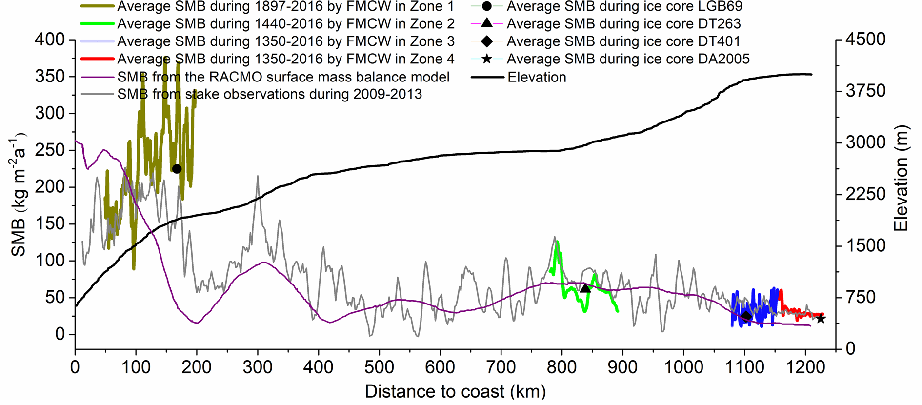
Fig. 7. Comparison of SMB estimates from different methods along the traverse route.
5.3. Temporal variations in accumulation
Three IRHs were used to study the temporal variability in the SMB along the traverse over each time period. The periods of ad 1897–1918, ad 1918–1928 and ad 1928–2016 are shown for zone 1 in Table 4 and Figure 5. The SMB profiles between the three time periods are similar (with an average SMB of 235 kg m−2 a−1 over ad 1897–2016), indicating that the climate has been relatively stable over the past 100 years in this region (Tables 6 and 7).
Table 6. Temporal variations in the average SMB at ad 1260–2016 for 18 km near ice core DT263

Table 7. Temporal variations in the average SMB at ad 883–2016 for 30 km near ice core DA2005

The Medieval Warm Period (MWP; 10th–14th centuries) and the Little Ice Age (LIA; 15th–20th centuries) are the two most recent climate events (Stenni and others, Reference Stenni2002), which can help understand the natural climate variability of Antarctica. Li and others (Reference Li, Cole-Dai and Zhou2009) speculated that LIA affected SMB only locally. The average SMB of zone 2 was 29 kg m−2 a−1 during ad 1440–1760, which is approximately one-third SMB of ad 1760–2016. SMB in zone 4 decreased by 20% between the 16th and 20th centuries (Table 4), but there was no significant change in the Dome A area. The limitation of IRH depth and the redistribution of snow may lead to distortion of IRH years (Frezzotti and others, Reference Frezzotti, Gandolfi and Urbini2002), so we only divide the transect region with less variable SMB near ice cores DT263 and DA2005 into six time periods for a more detailed temporal variation analysis (Tables 6 and 7).
During the MWP, the average SMB of zone 2 was 85 kg m−2 a−1 during ad 1260–1343 and decreased to 71 kg m−2 a−1 during ad 1343–1454. Furthermore, the average SMB was only 36 kg m−2 a−1 during ad 1454–1836. Then, it gradually increased through the 19th and 20th centuries to reach a modern SMB four times that of the LIA (145 kg m−2 a−1). This temporal pattern of change is similar to that which occurred at Talos Dome (Stenni and others, Reference Stenni2002).
Since the average SMB of zone 4 is only 29 kg m−2 a−1, the IRH depth after the 20th century is <10 m, which cannot be reliably identified in the radar-gram, so it is impossible to estimate the SMB temporal variations after the LIA. SMB increased from 22 to 35 kg m−2 a−1 during MWP and remained at 35 kg m−2 a−1 during ad 1511–1644, unlike zone 2. SMB in the Antarctic generally increased after the LIA (Bertler and others, Reference Bertler, Mayewski and Carter2011), but Dome A decreased to 27 kg m−2 a−1 during ad 1644–2016. SMB at Dome A showed an opposite trend to zone 2 during LIA, which may be related to the different distribution of moisture origins (Stenni and others, Reference Stenni2002). Broecker and others (Reference Broecker, Sutherland and Peng1999) pointed out that intense deep water formation may lead to the warming Antarctic during LIA.
To better understand the historical climate variability and its impact on SMB, it is necessary to expand spatial coverage of FMCW surveying in order to constrain time and space variability of SMB.
6. Conclusions
In the summer of 2015/16, a high-resolution FMCW radar was used to collect data along a 1236 km traverse from Zhongshan station to Dome A to examine the historical SMB record in this area for the first time. Through the analysis of the spatiotemporal variability in the internal radar stratigraphy, we demonstrated the following:
(1) The positions and depths of IRHs in the four distinct zones of the radar transect can be obtained from the radar-gram and the SMB variation characteristics can be obtained through calibration from ice core and stake data. The decreasing trend in the SMB with distance inland from the coast is evident in multiple datasets (stake arrays, ice cores, FMCW radar and RACMO).
(2) The shape of the IRHs is closely related to snowfall and surface snow redistribution. The decreasing trend in the SMB with distance inland from the coast is similar to that observed in Wilkes Land (Goodwin, Reference Goodwin1991) and Dome Fuji (Fujita and others, Reference Fujita2011). SMB in zone 1 is high, which is due to the proximity to the coast and the steep slope, resulting in high precipitation rates. Although the slope is high, the surface elevation over small distances (<5 km) does not fluctuate considerably, so the resulting SMB spatial variability is low. Zone 2 has a flat topography, but the measured SMB fluctuates spatially due to the formation of wind-induced surface features such as wind crusts. The SMB during the LIA (ad 1454–1836) was only one-quarter of that during the 20th century. The topography in zone 3 is much rougher than for the other transect regions and features erosion-induced ablation surfaces. Snow erosion and accumulation occur in this area under the influence of katabatic wind interactions with the surface topography, inducing sharp fluctuations in the IRH geometries. In zone 4 (i.e. the Dome A area), the slope, snow precipitation and wind speeds are the lowest of the entire traverse, and the observed IRHs are the flattest and showed an opposite trend to zone 2 during LIA.
(3) The maximum SMB error is estimated to be 3.56 kg m−2 a−1, and the most important factor is the error in the measured depth–density relationships. We obtain a strong correlation between modeled and observed densities at the ice core sites, with a maximum density error of 29 kg m−3 obtained at ice core site DT263. This error may be due to the redistribution of snow causing anomalies in the densification process.
Radar measurements can provide SMB over a large area of the ice sheet and can be used to analyze the spatiotemporal variability in SMB. In most areas, SMB data are still severely lacking for temporal analysis. To understand the Antarctic response mechanism to climate events such as the MWP and LIA, it is necessary to conduct such a temporal analysis in East Antarctica with results that may help constrain the state of the ice sheet under climate warming.
Author contributions
J. Guo and Y. Dou supervised the project. W. Yang, R. Dou, and Y. Zhang conducted the fieldwork and processed the data under Y. Dou's supervision. J. Guo performed all calculations and wrote most of the paper. W. Yang analyzed the FMCW data and contributed to writing the paper. Y. Pan collected data from the FMCW radar to measure the Antarctic ice sheet. X. Tang studied the calculation method of SMB. M. Ding provided the data of ice core LGB69. G. Shi provided the SMB data from stake observations during 2009–13. J. S. Greenbaum provided the data of the RACMO model, which helped us with model reliability analysis. All authors contributed to the development of the analyses, interpretation of the results, and extensive manuscript editing.
Acknowledgements
This work was funded by the National Key R&D Program of China (2018YFB1307504), the National Natural Science Foundation of China (41876227, 41776199, 41876230, 41776186), and the National Major Research Program (2013CBA01804). Field work was supported by the 32nd CHINARE, especially the inland expedition team. We also thank Mr Daqing Yang and Marie Cavitte anonymous reviewers for many helpful edits and comments. We thank Ms Shinan Lang for providing us with the radar principle and data processing help.
Data availability
All the data presented in the paper are available for scientific purposes upon request to the corresponding author (yangwangxiao0038@link.tyut.edu.cn).
Appendix A: converting TWT to depth
The transmitting antenna produces an electromagnetic wave and part of the wave is reflected when passing through a layer within the ice sheet. These reflected signals are received by the receiving antenna and are compared with the reference signal generated by the voltage-controlled oscillator to calculate the TWT of the electromagnetic wave based on the frequency difference. To convert TWT to depths in ice, TWT is divided by the speed of electromagnetic waves in ice (e.g. Yang and others, Reference Yang, Dou, Lang, Guo, Pan and Chen2019).
However, to assign ice core ages to the interpreted IRHs, real depths must be assigned to the IRHs. The firn/ice column, especially in the first 100 m, is a layered media composed of a mixture of air and firn (Kanagaratnam and others, Reference Kanagaratnam, Gogineni, Gundestrup and Larsen2001). As the depth increases, the air content in the firn continuously decreases. This densification process causes the density and crystal structure of the firn/ice to change. The permittivity is mainly influenced by density (Verfaillie and others, Reference Verfaillie2012). As shown in Eqn (A1), this process affects the electromagnetic wave velocity. However, the electromagnetic wave velocity is needed to convert the TWT to depth. The electromagnetic wave propagation in a given medium is described as follows:

where c v is the wave velocity in a vacuum (i.e. 0.3 m ns−1) and the wave velocity c in the medium (firn/ice) is directly affected by the permittivity ɛ.
The density of ice increases with depth and the rate of this change gradually slows after exceeding a critical density (830 kg m−3) (Ren and others, Reference Ren, Qin and Xiao2001). Assuming that there are no jumps in the density change trend, the Looyenga (Reference Looyenga1965) model is used to calculate the dielectric permittivity of such layered media according to

where ɛ2 is the dielectric constant of ice (i.e. 3.15; Kanagaratnam and others, Reference Kanagaratnam, Gogineni, Gundestrup and Larsen2001), ɛ1 is the dielectric constant of air (i.e. 1), and v is the volume fraction of ice in the firn obtained by the following equation:

where ρ is the density of the firn and ρ i is the density of pure ice (i.e. 918 kg m−3; Kanagaratnam and others, Reference Kanagaratnam, Gogineni, Gundestrup and Larsen2001).
Finally, by introducing Eqns (A1) and (A3) into Eqn (A2), we obtain the following expression:

Using Eqn (A4), the change in electromagnetic wave velocity over the vertical profile is calculated using the density–depth relationship measured in the field (see Section 2.2).


 Open access