The Use of Evolutionary Methods for the Determination of a DC Motor and Drive Parameters Based on the Current and Angular Speed Response


Abstract
:
1. Introduction
- Determination of seven DC motor and drive parameters only based on speed and current responses. We tested different evolutionary methods, while other authors used only one standard or evolutionary method. The most appropriate evolutionary method between those selected is proposed based on tests.
- Different parameters can be determined with the presented approach: Only the motor (parameters of the motor and inertia and friction of the motor), DC motor drive without load (parameters of the motor and inertia and friction of the drive), DC motor drive with the load (parameters of the motor and inertia of the drive and load characteristic of the drive).
- The method is also extended for the motor and drive parameter determination in the case of a controlled drive. The influence of a speed controller on the current and speed responses is considered in the DC motor model with the use of the measured voltage. Also, current limitation of the supply unit is considered in the DC motor model. Such an approach has not been found in the literature, as mostly authors use step responses of speed and current, or, in the case of controlled drive, they use a model of the controller.
- The accuracy of the DC motor model, used for the Objective Function calculation, is improved by dividing the time step of the measurement, which cannot be reduced, into smaller steps in the Objective Function calculation. Such approach to improve the accuracy of the calculation was not found in the literature.
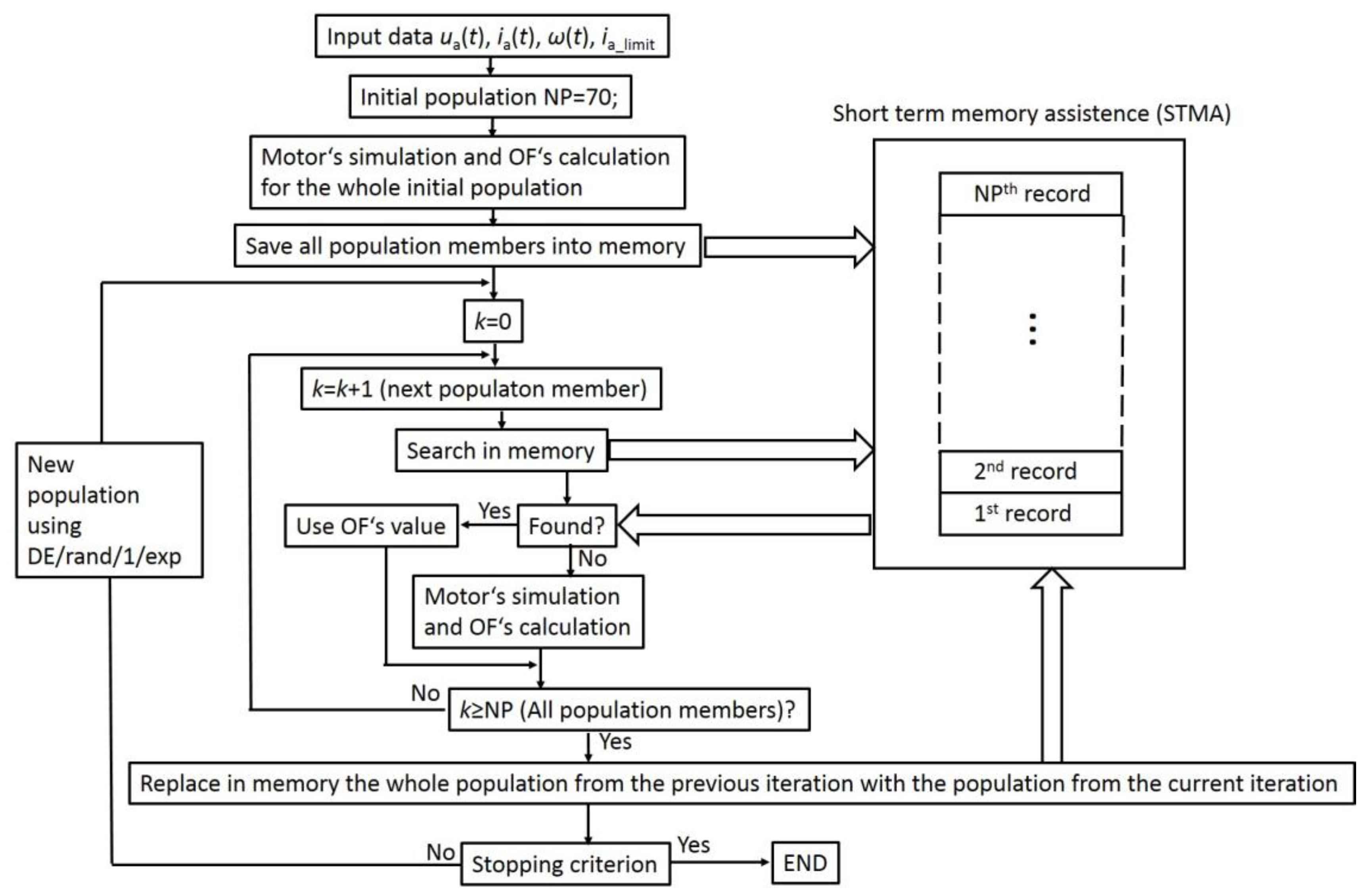
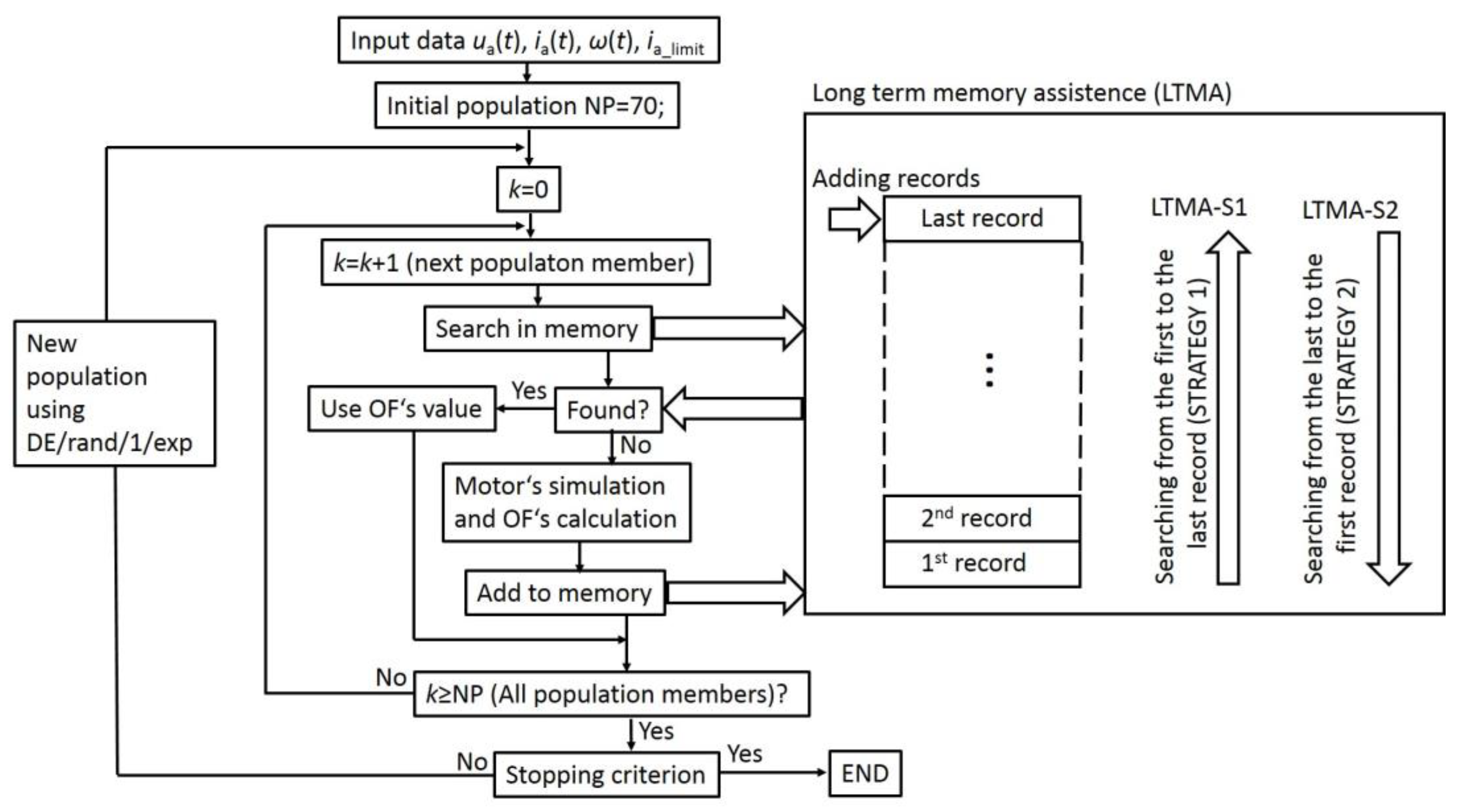
- To reduce calculation time short-term memory assistance (STMA) is used, which records not only the current population, but also population from the previous calculation step. Also presented is long-term memory assistance (LTMA), which records the entire search history. In the case of LTMA two different search strategies are used for the search in history.
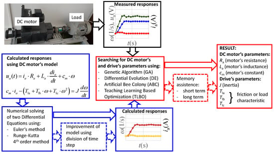
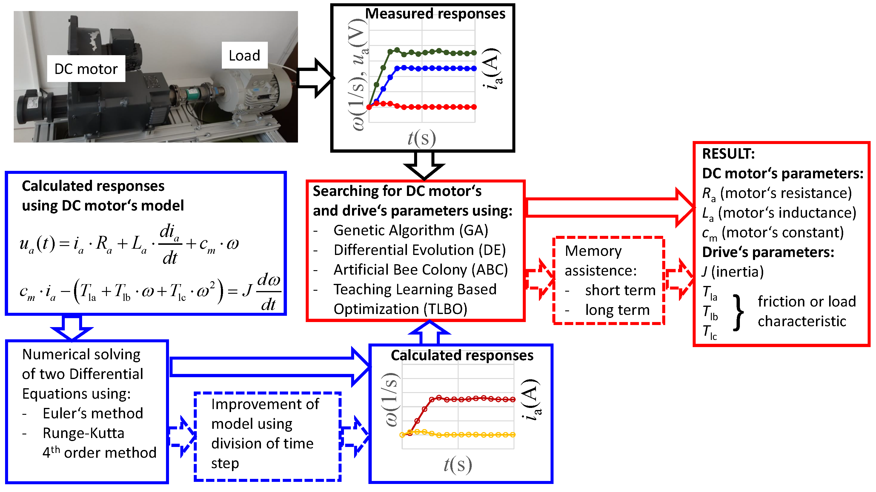
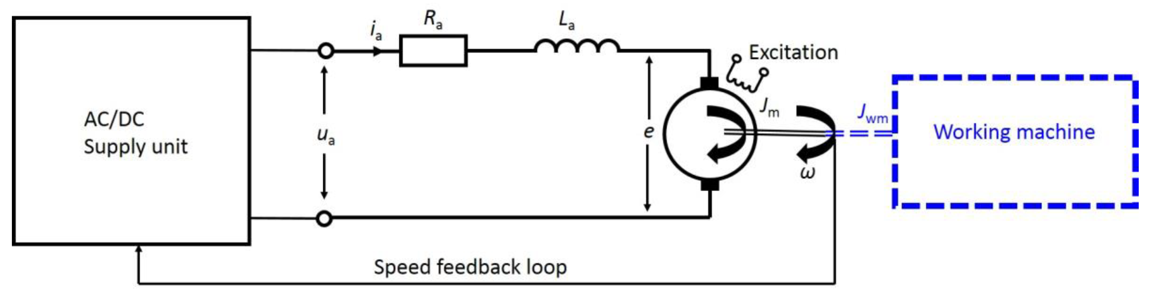
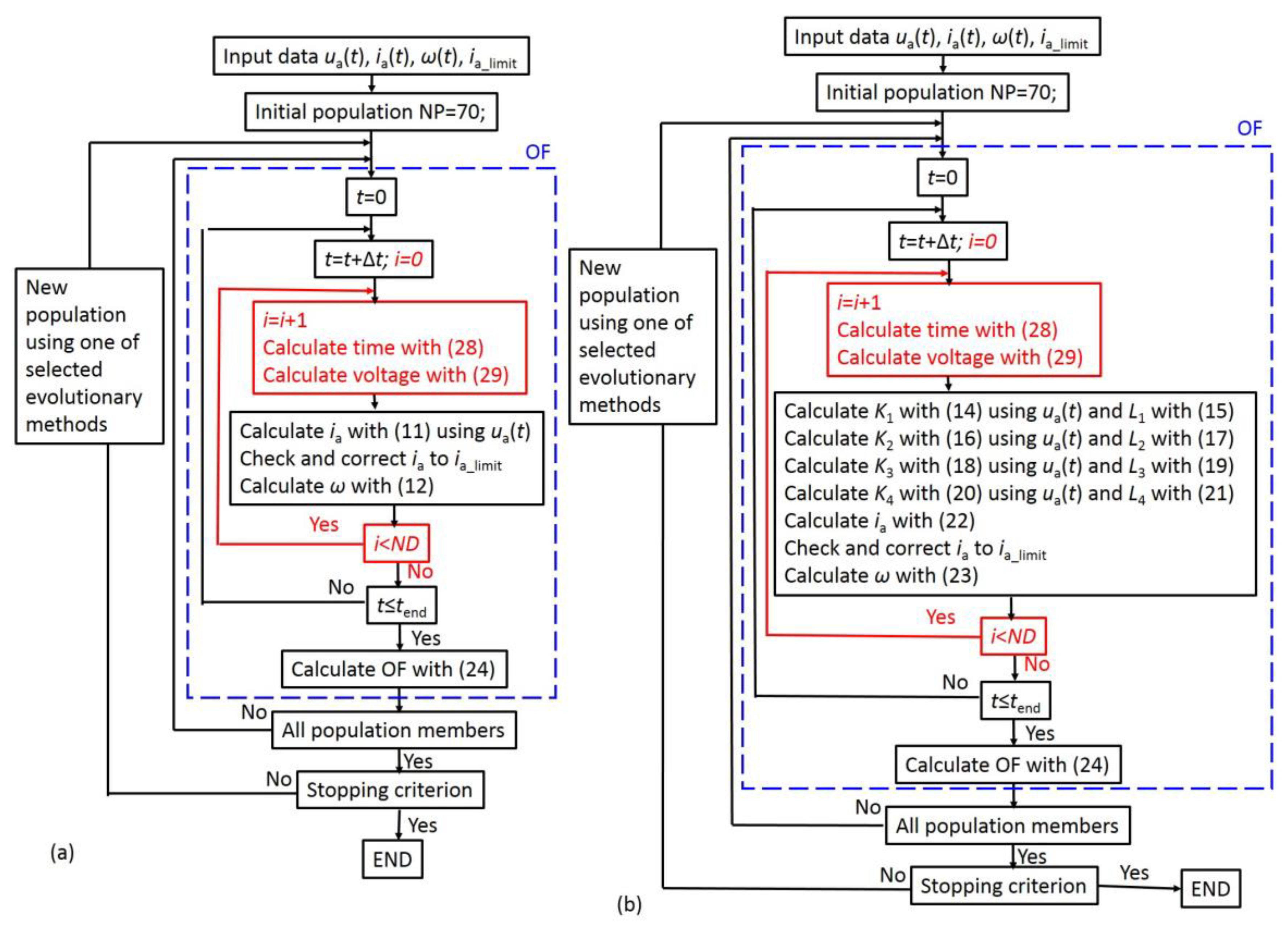
2. Principle of Parameter Determination
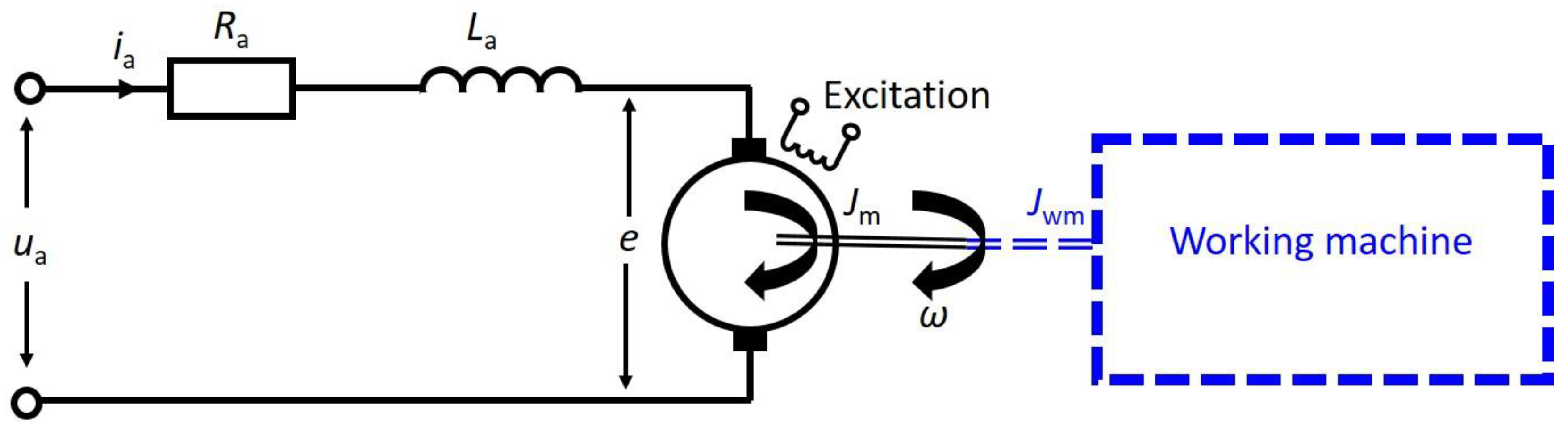
2.1. DC Motor Model and Simulations
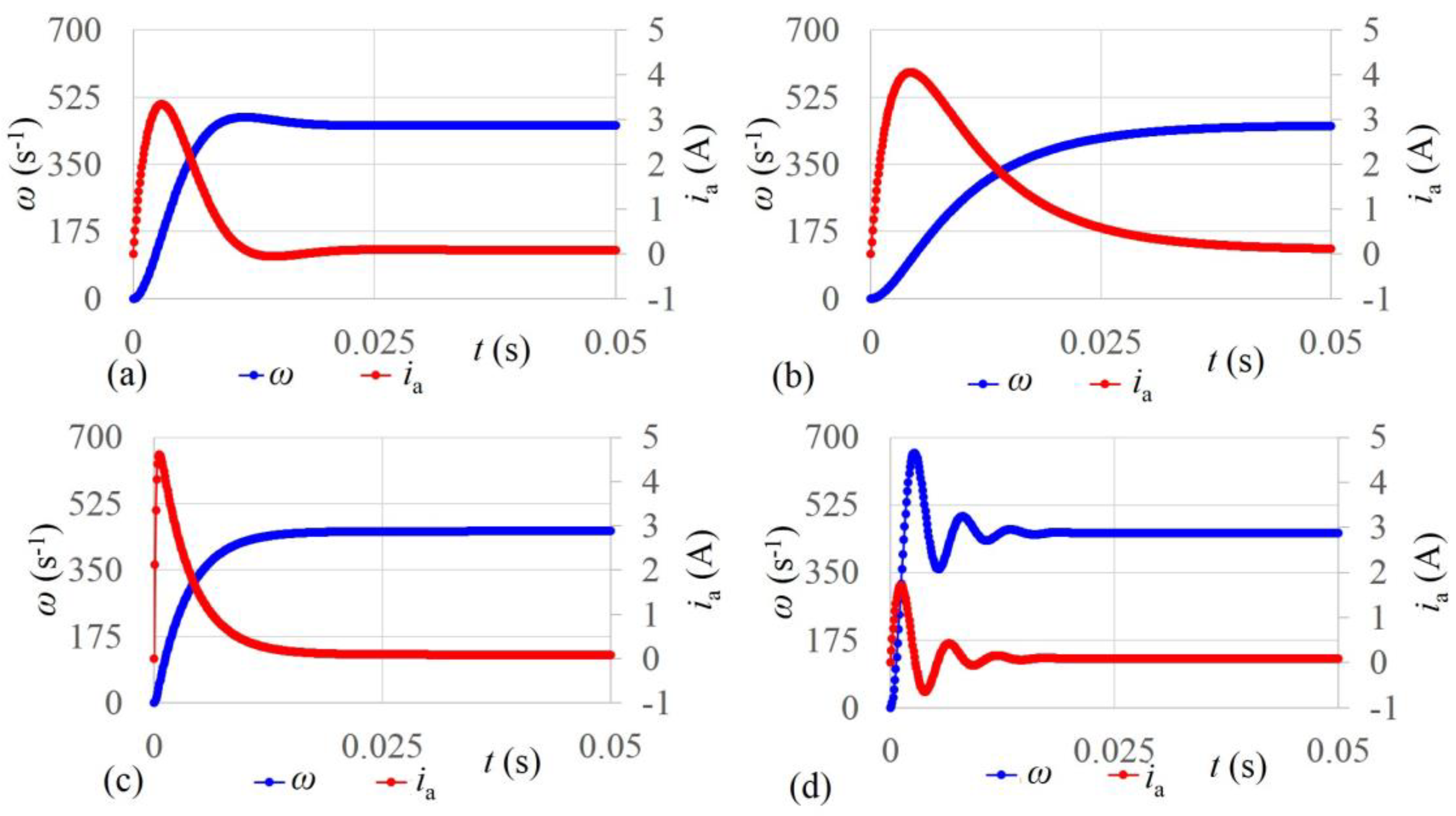
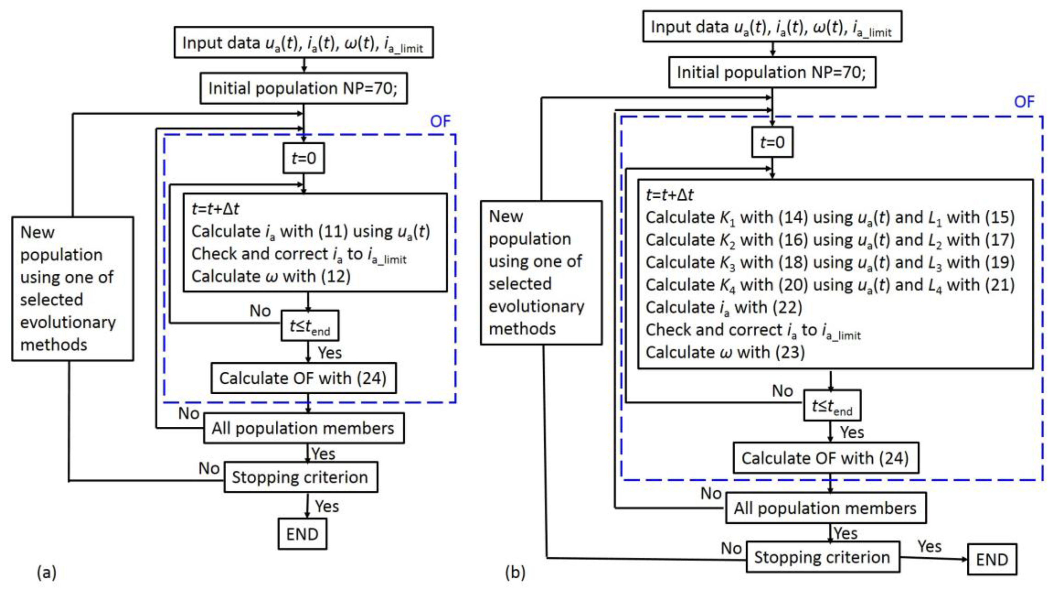
2.1.1. Simulation with the Use of Euler’s Method
2.1.2. Simulation with the Use of Fourth-Order Runge–Kutta Method
2.2. Methods for Parameter Determination
3. Simulated Data Used as Input
- The weaknesses of the model are avoided. For example, La is not a completely constant value, but it is considered to be a constant value.
- The phenomena, which are not covered by the model, such as armature reaction, is eliminated from the input data.
- The exact values of all seven parameters, which should be obtained as results, are known, because they are used as input for preparation of the simulated current and speed step responses.
- The same method (the fourth-order Runge–Kutta method) is used to prepare simulated input data and to evaluate the OF (24) during the parameter determination process. With that, the influence of the selected method on the results is eliminated.
3.1. Results Obtained Using Simulated Input Data
- Mean values of parameters calculated using DE/rand/1/exp are the same as the values used to generate input data. These results are the best.
- Mean values of the parameters calculated using TLBO are almost the same as the values used to generate input data. The small difference is only for the parameters describing load, which are Tla, Tlb, and Tlc.
- Mean values of the parameters calculated using GA, DE/best/1/bin and ABC are more or less different than the values used to generate input data.
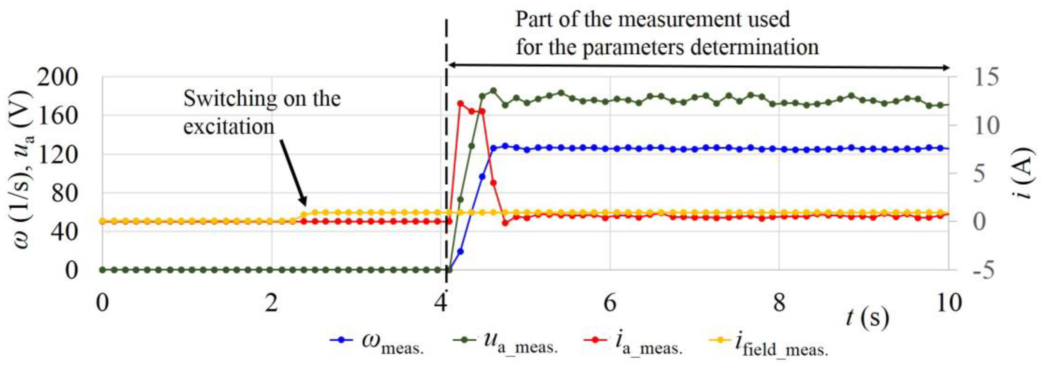
4. Measured Data Used as an Input and Improvement of the Method for Controlled Drive and Current Limitation
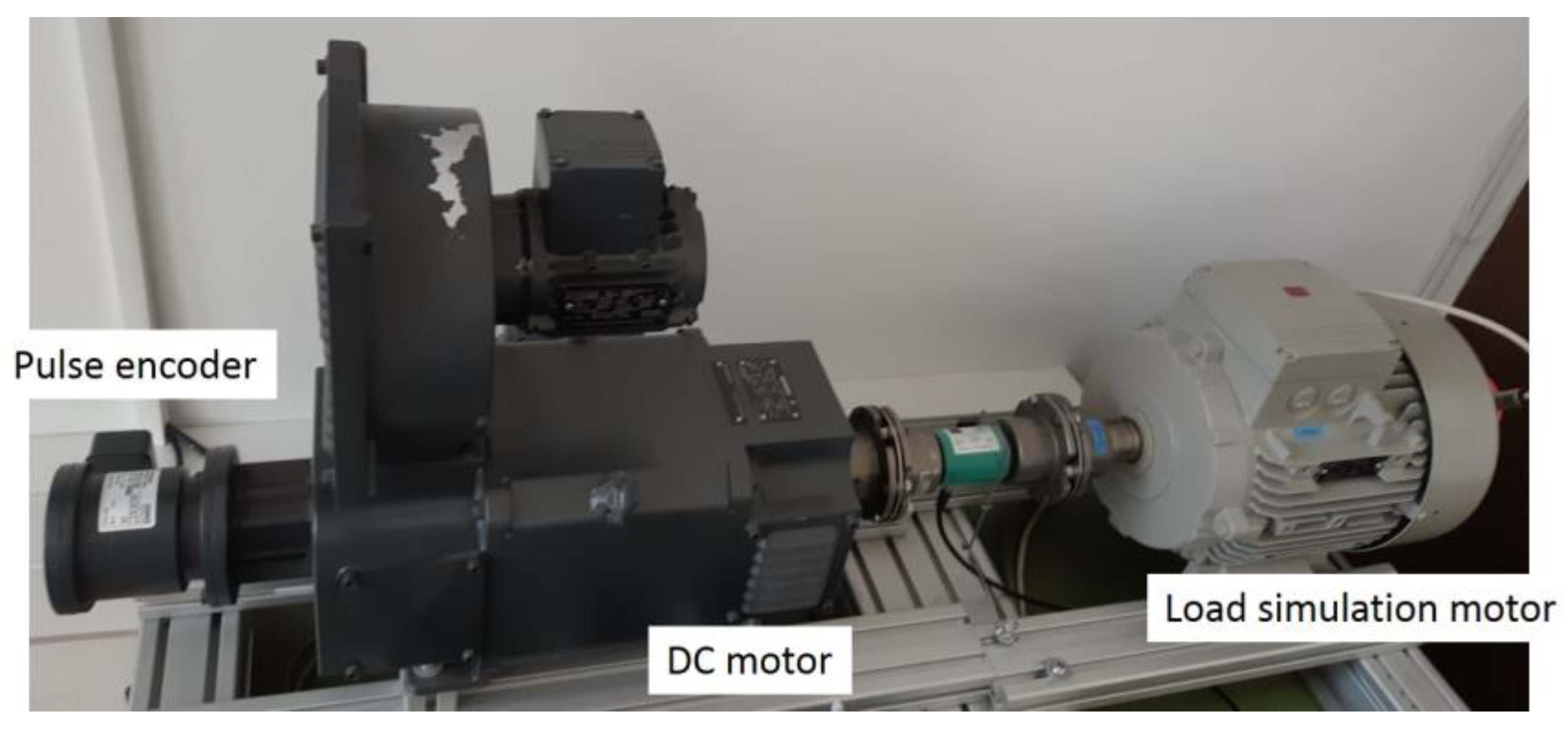
4.1. Measured Data Used as a Test Example
- Supply unit: SIEMENS SIMOREG DC-Master 6RA7013-6DV62-0-Z.
- DC motor: SIEMENS 1GG5104-0ED40-6VV1.
- Pulse encoder: HUBNER Berlin, P0G 9D 1024.
- Load simulation motor: SIEMENS 1LA7139-4AA10-Z FDB0
- Measurements were made with the use of a “Trace” function, which is a part of the SIEMENS “Drive Monitor” software used for supply unit support.
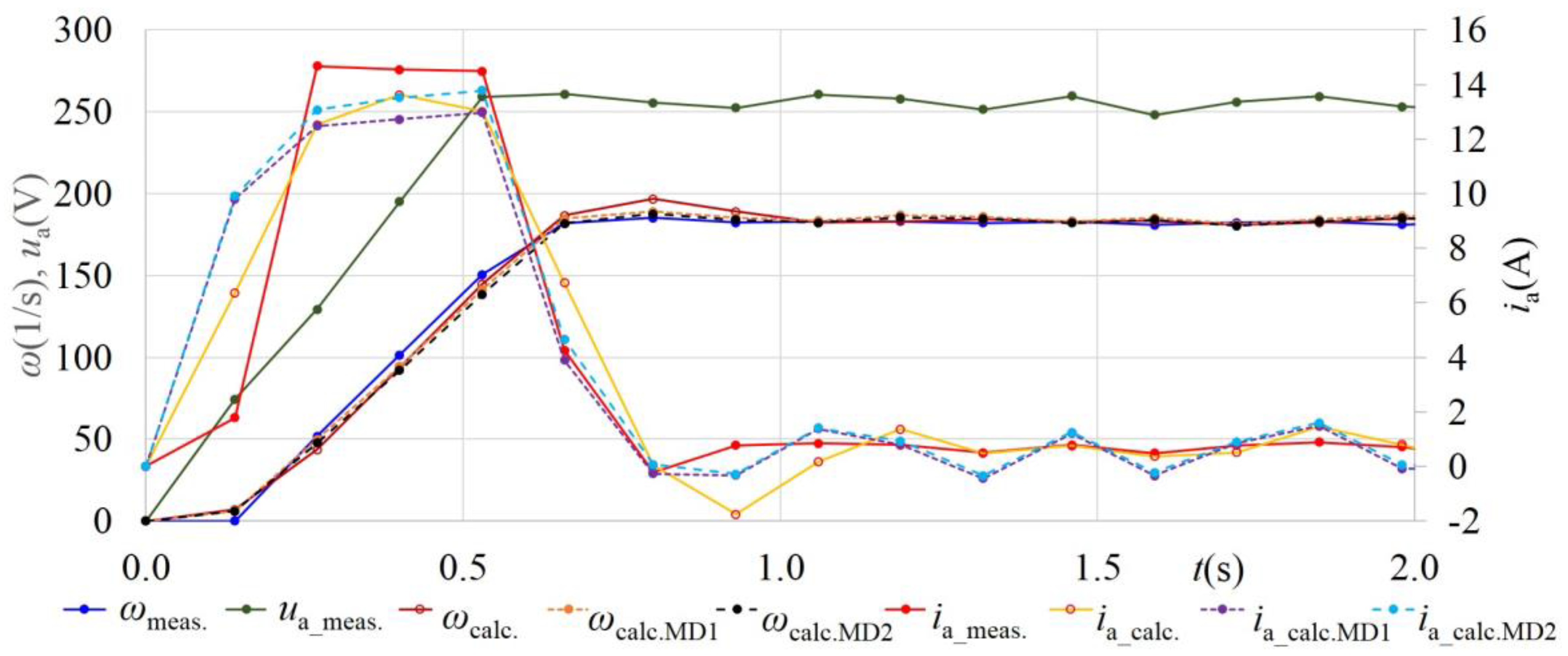
4.2. Results Obtained Using the Measured Input Data
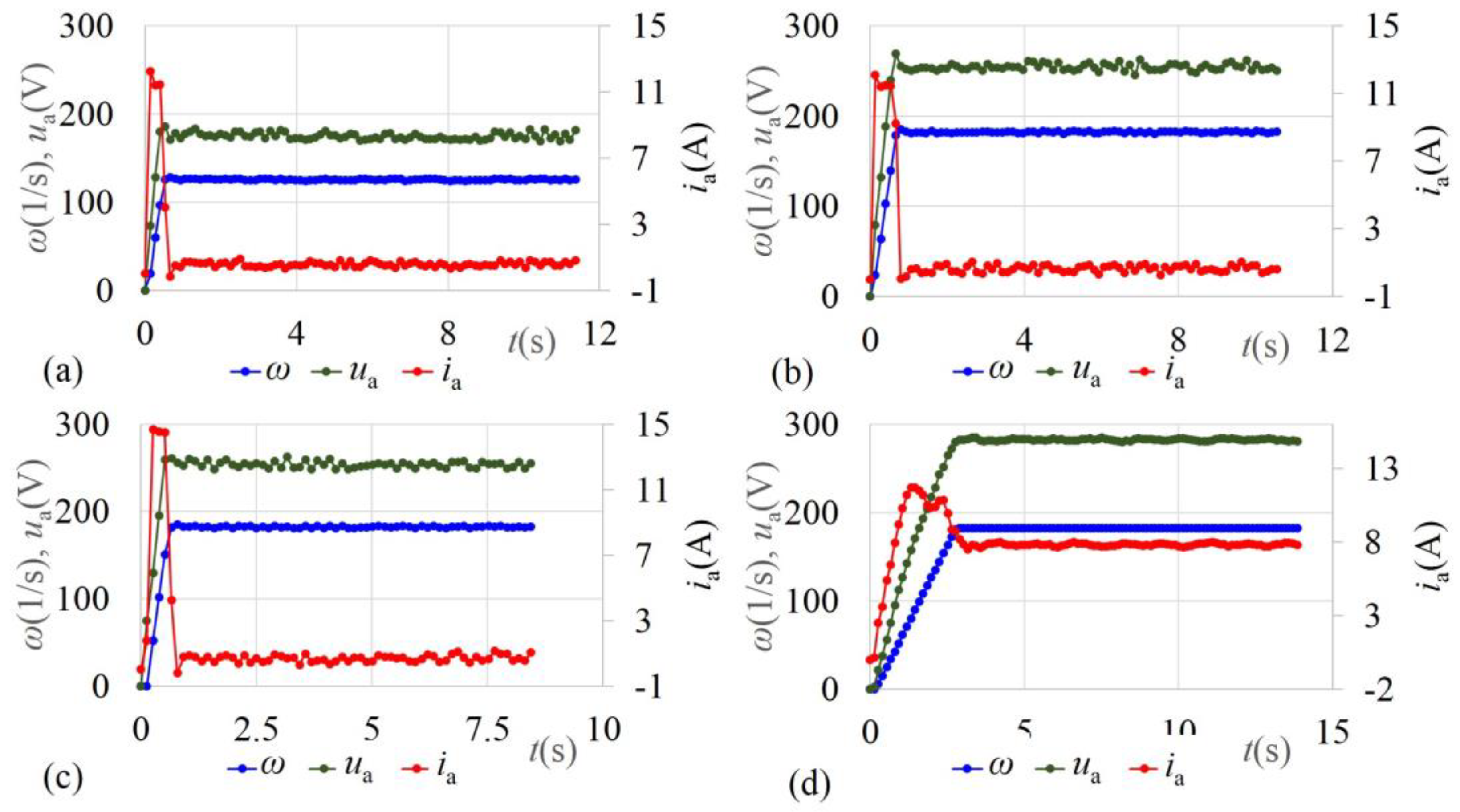
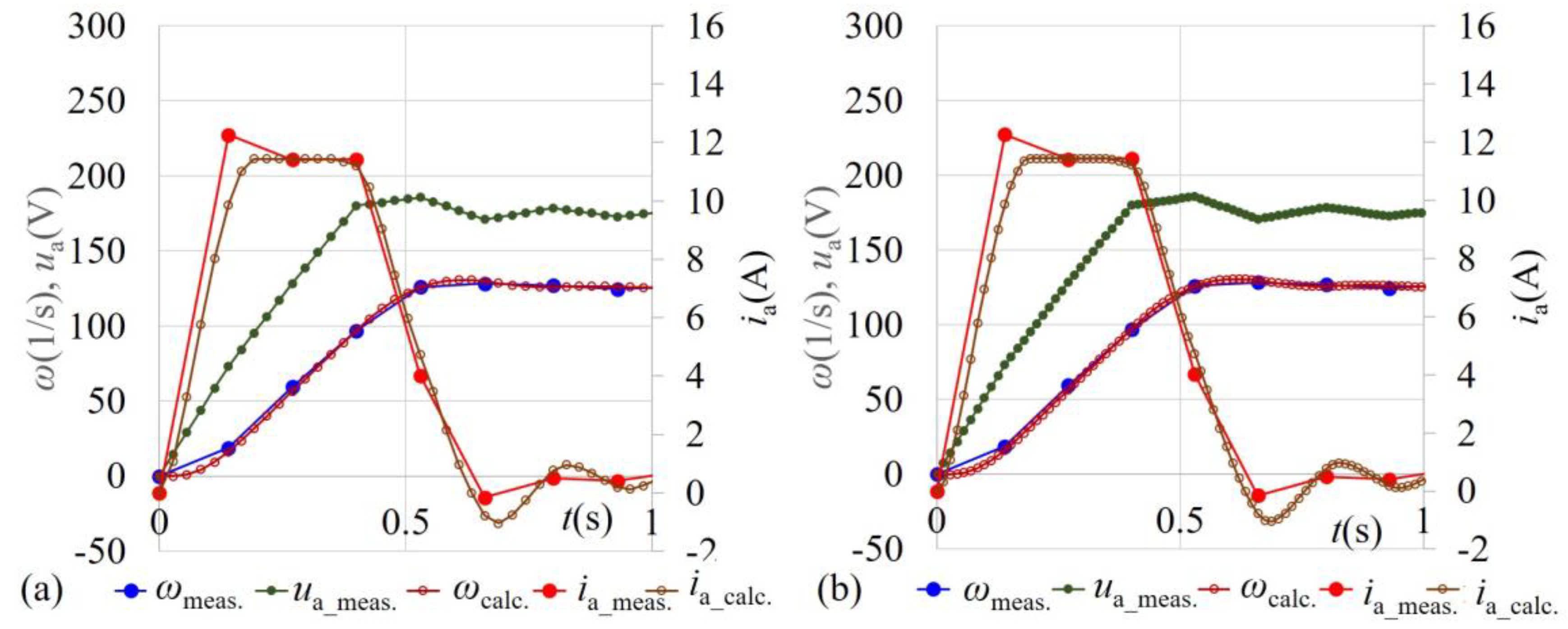
4.2.1. Results Obtained Using Input Data MD1
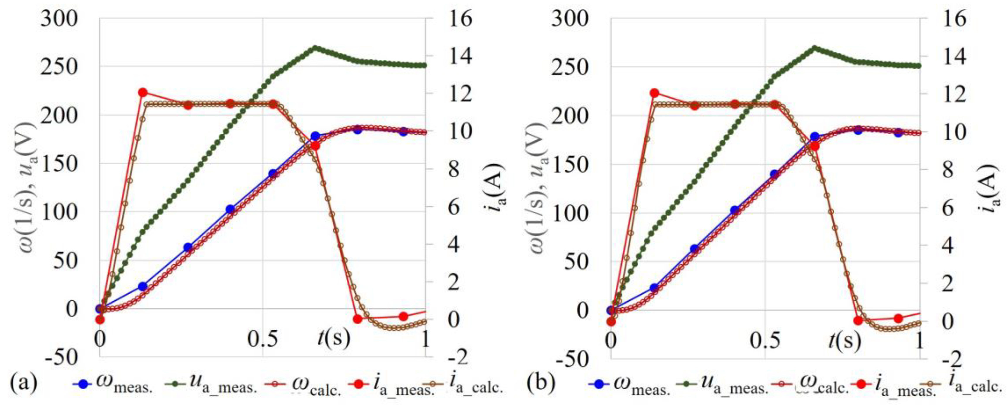
4.2.2. Results Obtained Using Input Data MD2
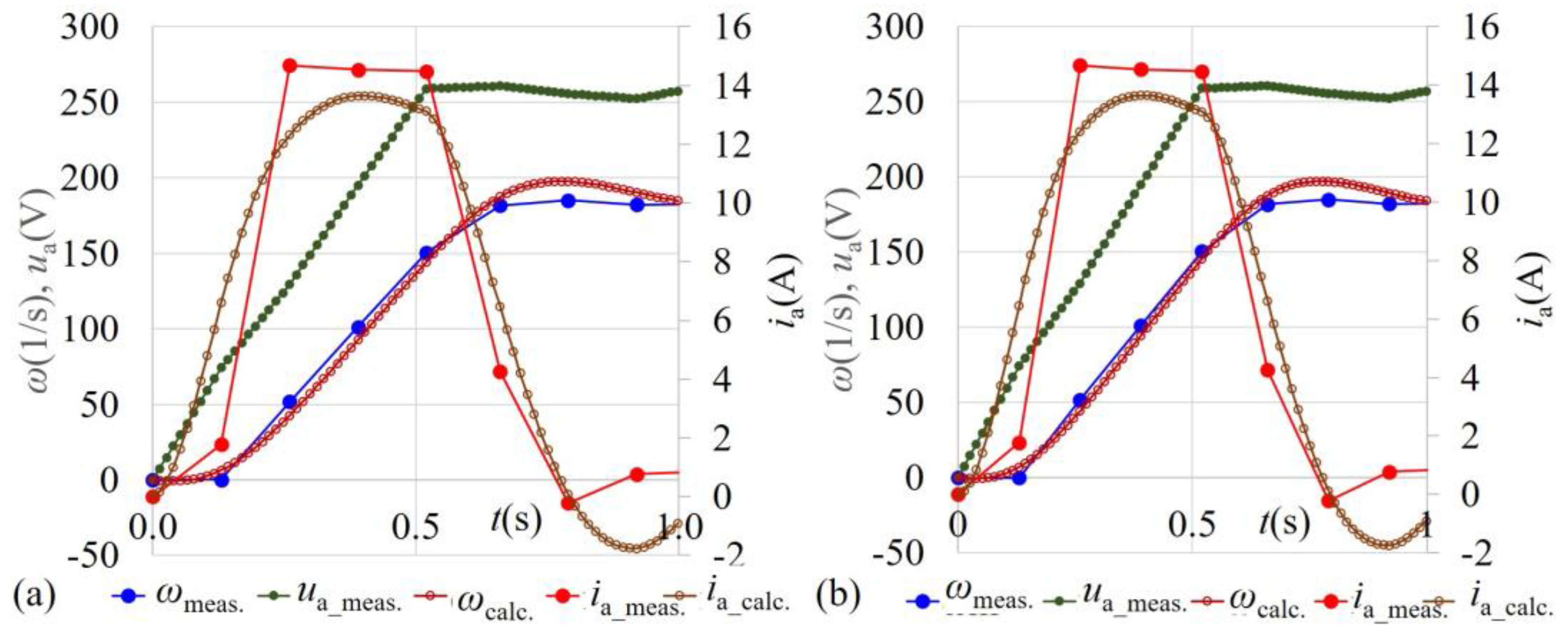
4.2.3. Results Obtained Using Input Data MD3
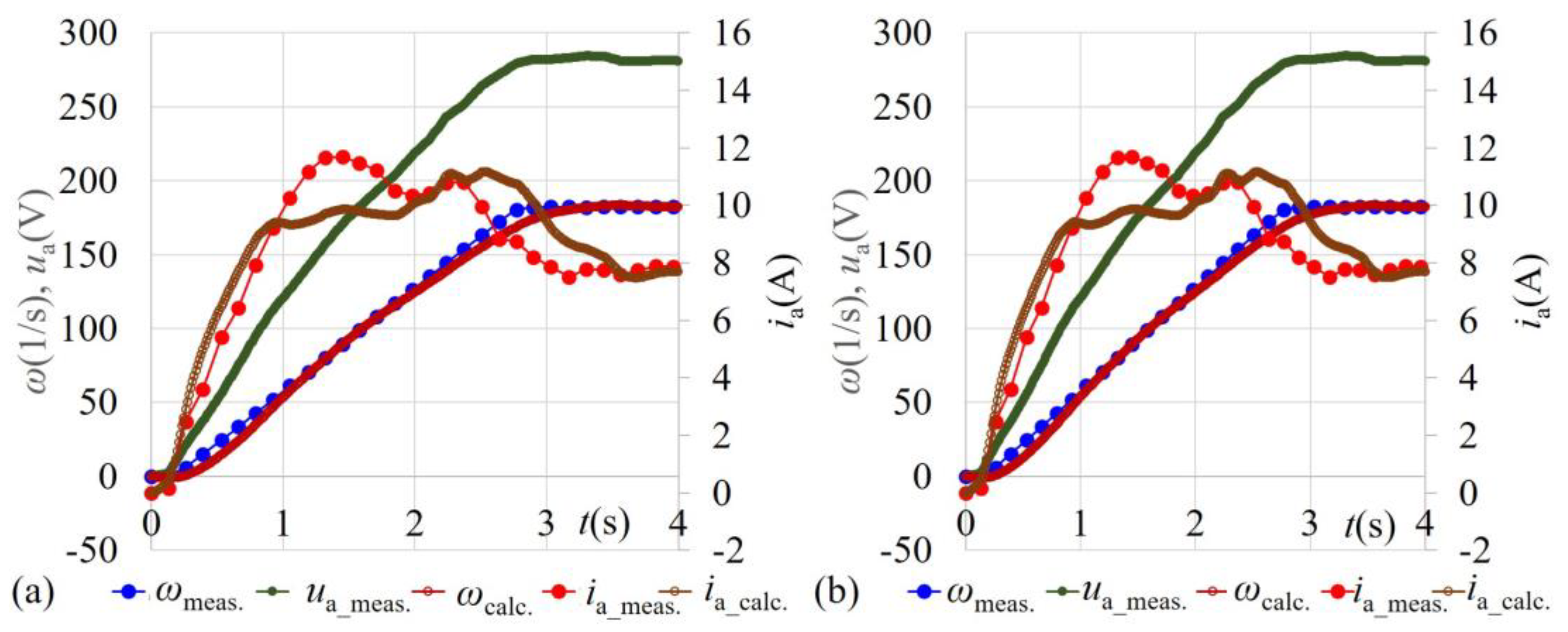
4.2.4. Results Obtained Using Input Data MD4
4.2.5. Comparison of Results Obtained Using All Four Input Data Sets
- Ra: The maximum deviation of calculated Ra was less than 14%, which is a good result.
- La: Calculated La was between 244 mH and 451 mH, the difference was due to the deviations in measurements. As can be seen from the result, a small deviation in the measurement causes a significant change of La.
- cm: Calculated cm was between 1.314 and 1.376, which is a good result, because the difference between calculated values was less than 5%.
- J: The real inertia of the drive was approximately 0.04 kgm2 (inertia of some small parts is not known). The calculated inertia was in the range of 20% in the cases of MD1, MD2, and MD3. Only in the case of MD4, was the calculated inertia too small, due to the deviations of the measurements (see a more detailed explanation in Section 4.2.4).
- Tla: Parameter Tla was a friction of the drive, which was approximately 0.9 Nm. The calculated values for all four input data were in the scope of 15%.
- Tlb, Tlc: Parameters Tlb and Tlc were negligibly small in cases MD1, MD2, and MD3. In the case of MD4 load was present, which was linearly dependent on speed. The total load at angular speed 182 s−1 was approximately 14.6 Nm. The calculated load considering parameters Tla, Tlb, and Tlc was 10.1 Nm, which was a deviation of 31%.
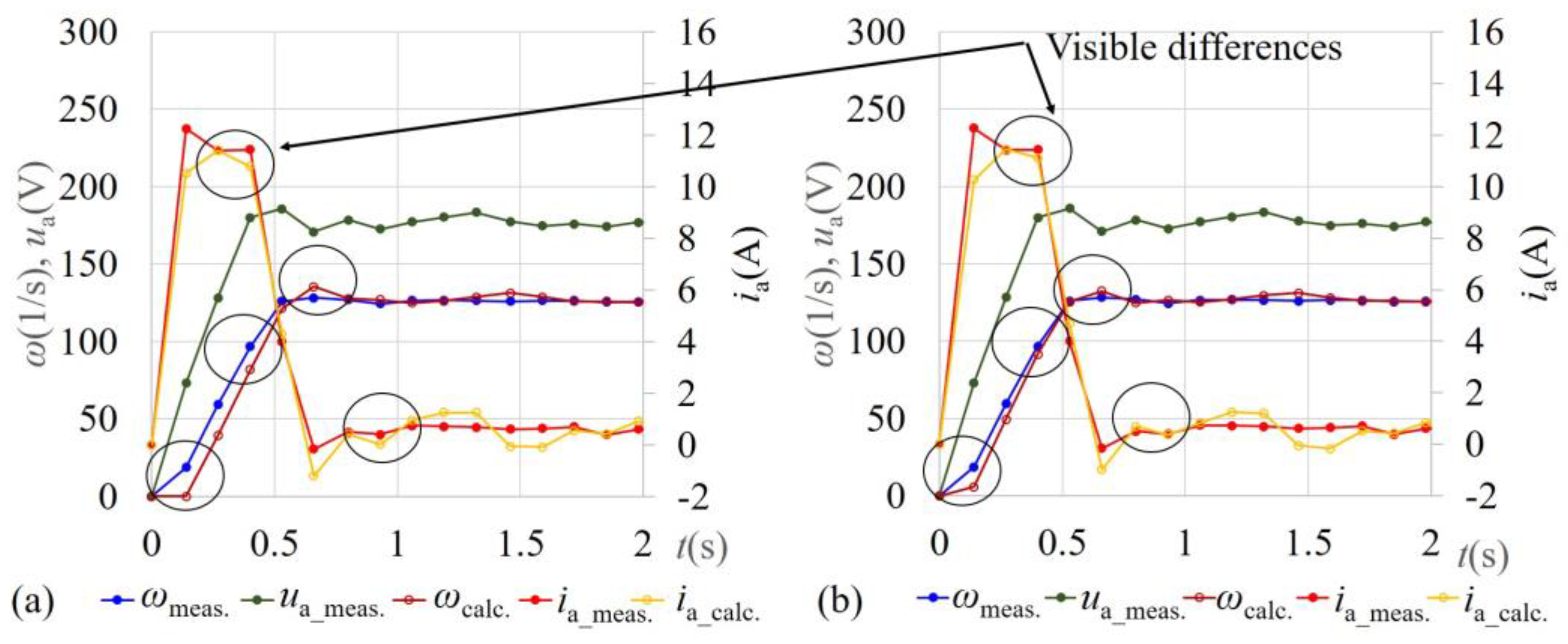
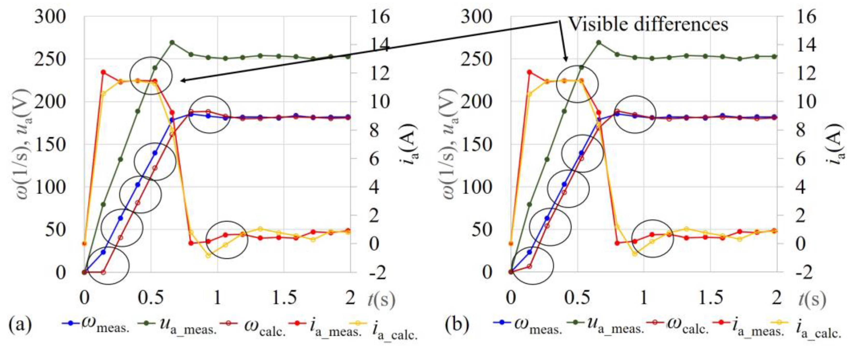
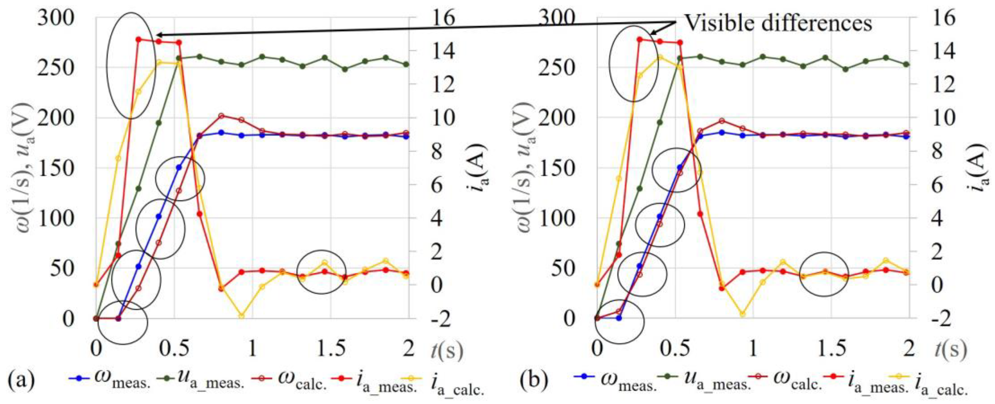
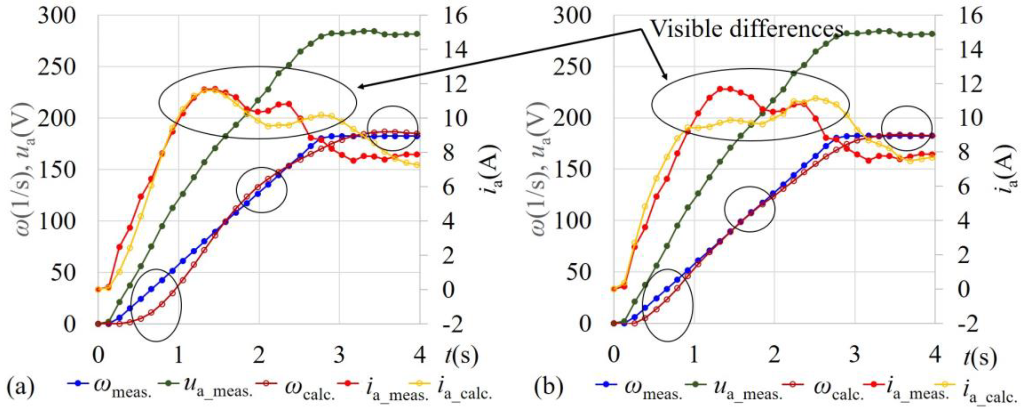
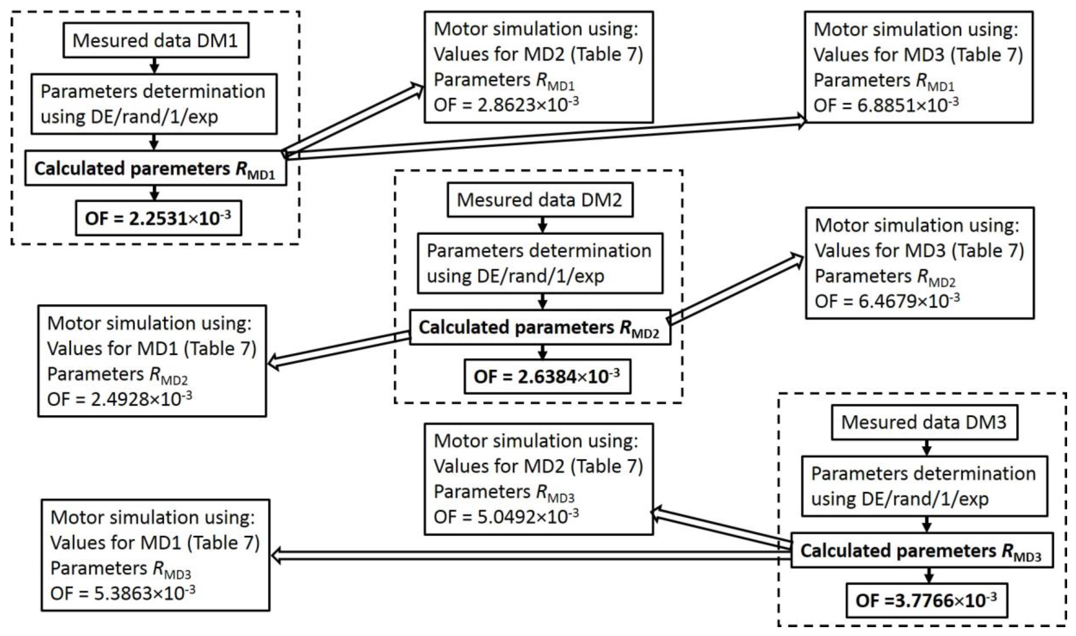
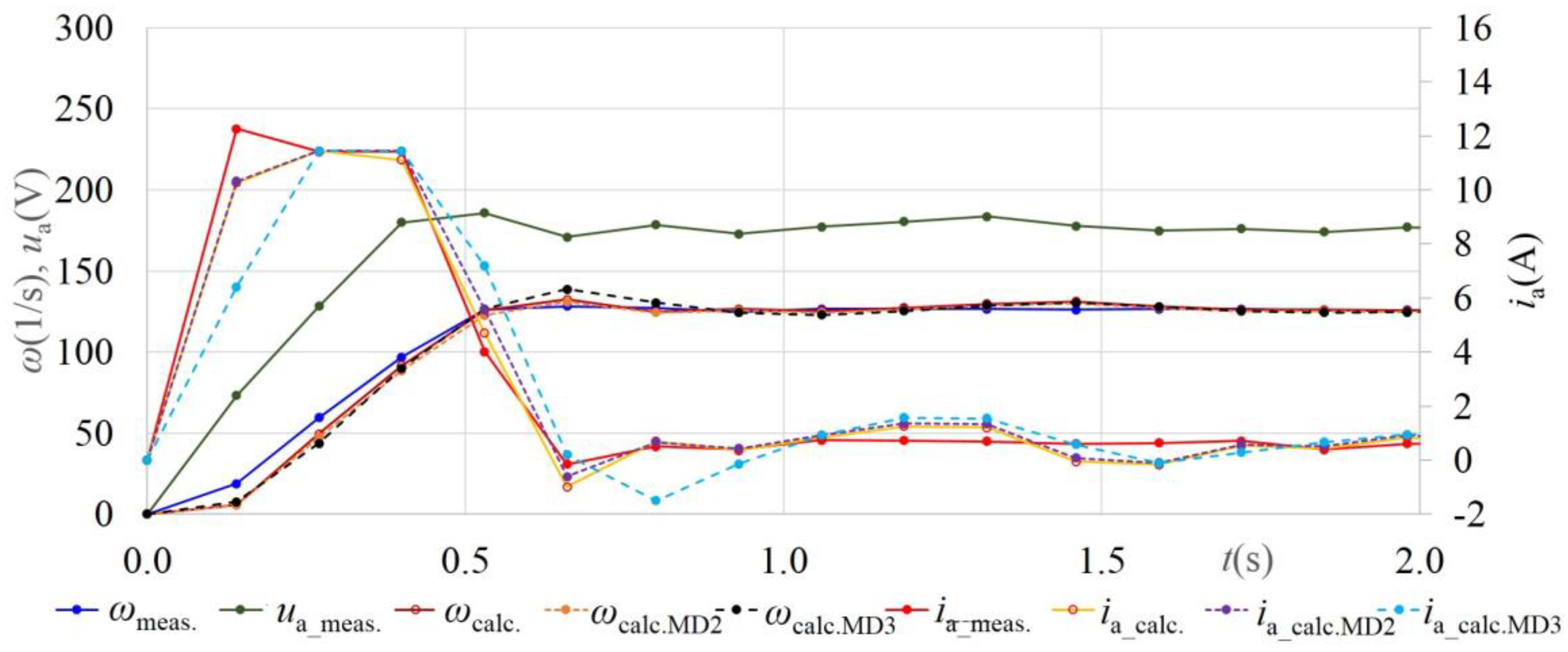
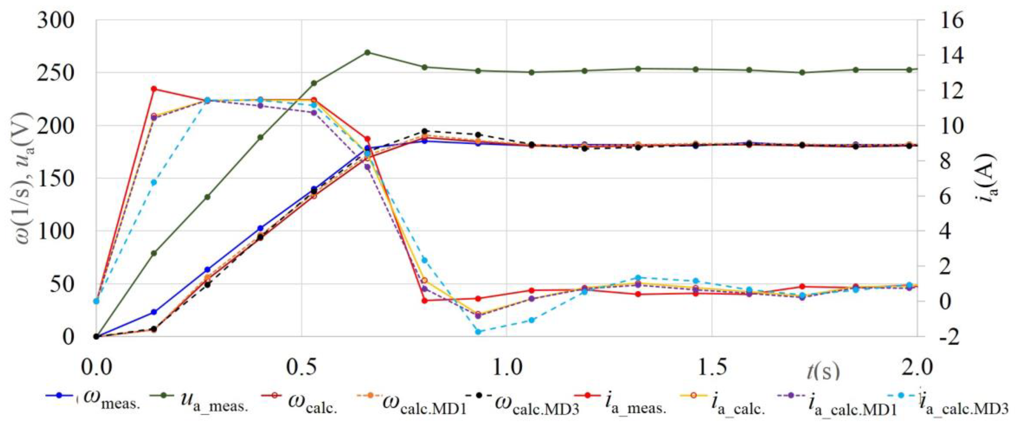
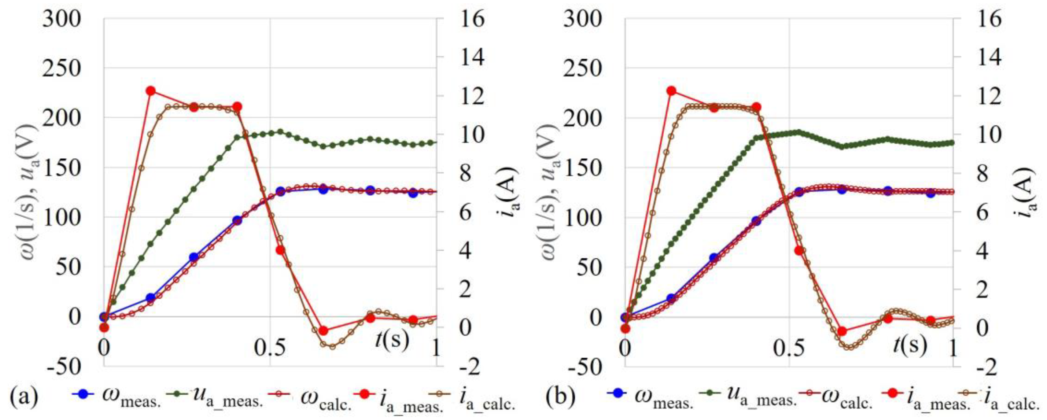
4.2.6. Cross-Validation of the Obtained Results
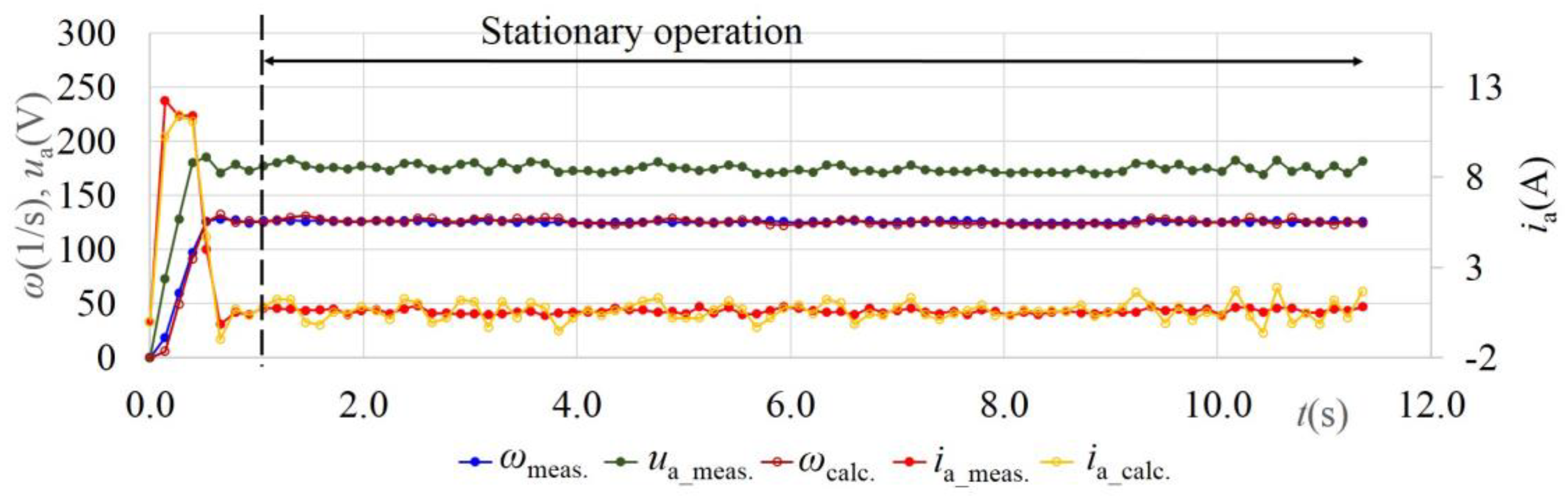
4.2.7. Testing of Result Correctness at Stationary Points
4.2.8. Calculation Times
- Calculation times were mostly longer for a higher number of measured points (MD1 87, MD2 81, MD3 65, MD4 106 measured points), which was the expected result.
- Calculation times using RK were mostly approximately not more than 25% longer than calculation times using EM, although in the case of RK, ten expressions (14)–(23) were calculated for each time instant, and in the case of EM, only two expressions (11) and (12) were calculated for each time instant.
- Calculation times using different evolutionary methods were different. The fastest was GA. The calculation times of DE were 20 to 40% longer than the times of GA. Calculation times of TLBO and ABC were 100 to 150% longer than the calculation times of DE.
4.2.9. Influence of Weights Used in OF on Results
- In the case of MD1, correct results (due to the known values written at the bottom of Table 20) are obtained for weights w1 ≥ 0.5. For w1 ≤ 0.4, parameter Tla has an incorrect value. For higher w1, slightly better results were obtained, for example Ra at w1 = 0.5 is 5.06 and at w1 = 0.9 it is 5.34.
- In the case of MD2, correct results were obtained for weights w1 ≥ 0.4. For w1 ≤ 0.3 parameter, Tla has an incorrect value. For higher w1, slightly better results were obtained, for example, Ra at w1 = 0.4 is 4.87 and at w1 = 0.9 it is 5.24.
- In the case of MD3 correct results were obtained for weights w1 ≥ 0.4. For w1 ≤ 0.3 parameter, Tlc has an incorrect value. For higher w1, almost no difference in results was obtained, for example, Ra at w1 = 0.4 is 4.86 and at w1 = 0.9 it is 4.91.
- In the case of MD4, only results for w1 = 0.4 and 0.5 are acceptable. For w1 ≤ 0.3, Tla is too small, and for w1 ≥ 0.6, T1a is too big.
4.3. Motor Model Simulations with Time Interval Division
4.4. Analysis of Memory Assistance
- STMA: In each iteration, population members are compared with members from only one previous iteration. After each iteration, the whole population is saved into memory. Only additional memory for one population set is used using the presented approach. In the presented case, this is ((7 parameters + OF) × 70 population members) memory locations.
- Long-Term Memory Assistance—Strategy 1 (LTMA-S1): Each population member is compared with all members written into memory, obtained from all previous iterations. Each member which is not found in the memory is added to the memory. Strategy 1 means that the search in the memory starts from first added to the last added (when the same population member is found, the search is finished). Theoretically ((7 parameters + OF) × 70 population members × 2000 iterations) locations of additional memory can be used.
- Long-Term Memory Assistance—Strategy 2 (LTMA-S2): It is the same as LTMA-S1, only the strategy of the search is changed. It starts from the last added to the first added.
- Duplications for STMA were between 50–60% for MD1 and MD2, between 35–60% for MD3 and between 30–40% for MD4.
- Duplications for LTMA (S1 and S2) were between 75–86% for MD1, MD2, and MD3 and between 67–78% for MD4.
- Based on previous remarks, it can be seen that in the case of LTMA, the number of duplications was much higher than in the case of STMA, which was expected. It is interesting that duplications depend not only on precision, stopping criteria, type of problem, etc., but also on input data.
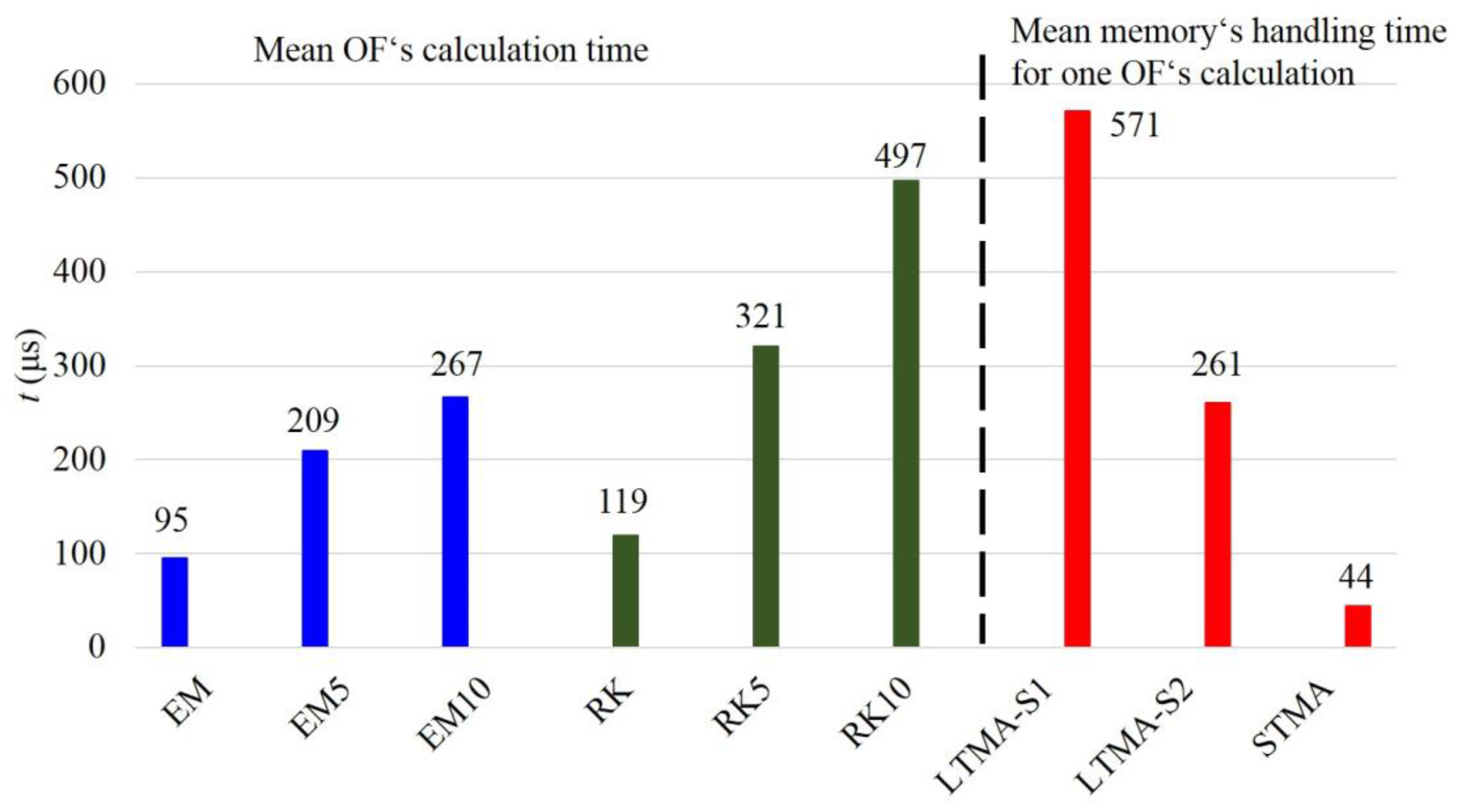
- Calculation times using STMA were, in the cases of EM and RK, in the range from 94.3% up to 109% of times without Memory Assistance, so the time was only a little shorter or even longer. In the cases of EM5, EM10, RK5, and RK10, times were shortened up to 51.1% of times without Memory Assistance.
- Calculation times using LTMA-S1 were longer than times without Memory Assistance. They were in the range from 104.6% in the case of RK10 (MD1 and MD4), up to 431.4% in the case of EM (MD4). The presented problem is not time-consuming enough to be suitable for LTMA-S1.
- Calculation times using LTMA-S2 were longer than times without Memory Assistance in the cases of EM, EM5 and RK, in the range from 104.2% in the case of EM5 (MD1) up to 240.1% in the case of RK (MD4). In the cases of EM10 and RK5, times were in some cases shorter and in some longer. They were in the range from 78.2 up to 132.4%. The shortest times were obtained in the case of RK10, which was the most time-consuming method. They were in the range from 56.8 up to 64.3% for MD1, MD2, and MD3, which were even shorter than the times in the case of STMA. Only in the case of MD4, where the number of duplications is smaller, was the calculation time 91.3%, which was a longer time than in the case of STMA.
5. Conclusions
Author Contributions
Finding
Conflicts of Interest
References
- Wu, W. DC Motor Parameters Identification Using Speed Step Response. Model. Simul. Eng. 2012, 2012, 189757. [Google Scholar] [CrossRef] [Green Version]
- Adewusi, S. Modeling and Parameters Identification of a DC Motor Using Constraint Optimization Technique. IOSR J. Mech. Civ. Eng. 2016, 13, 46–56. [Google Scholar]
- Avoda, M.L.; Ramzy, S.A. Parameter Estimation of a Permanent Magnets DC motor. Iraqi J. Electr. Electr. Eng. 2019, 15, 28–36. [Google Scholar] [CrossRef]
- Hadef, M.; Bourouina, A.; Mekideche, M.R. Parameters Identification of DC Motor via Moments Method. Iran. J. Electr. Comput. Eng. 2008, 7, 159–163. [Google Scholar]
- Hadef, M.; Mekideche, M.R. Parameter identification of a separately excited dc motor via inverse problem methodology. Turk. J. Electr. Eng. Comp. Sci. 2009, 17, 99–106. [Google Scholar]
- Shanmuga, N.B.; Mythile, A.; Pavithra, S.; Nivetha, N. Parameter Identification of a DC Motor. Int. J. Sci. Technol. Rese. 2020, 9, 5746–5755. [Google Scholar]
- Sankardoss, V.; Geethanjali, P. Parameter estimation and speed control of a PMDC motor used in wheelchair. Energy Procedia 2017, 117, 345–352. [Google Scholar] [CrossRef]
- Amiri, M.S.; Ibrahim, M.F.; Ramli, R. Optimal parameter estimation for a DC motor using genetic algorithm. Int. J. Power Electr. Drive Syst. 2020, 11, 1047–1054. [Google Scholar] [CrossRef]
- Dupuis, A.; Ghribi, M.; Kaddouri, A. Multiobjective genetic estimation of DC motor parameters and load torque. In Proceedings of the IEEE International Conference on Industrial Technology, 2004. IEEE ICIT ′04, Hammamet, Tunisia, 8–10 December 2004. [Google Scholar] [CrossRef]
- Puangdownreong, D.; Hlungnamtip, S.; Thamarat, C.; Nawikavatan, A. Application of flower pollination algorithm to parameter identification of DC motor model. In Proceedings of the 2017 International Electrical Engineering Congress, Pattaya, Thailand, 8–10 March 2017. [Google Scholar] [CrossRef]
- Goldberg, D. Genetic Algorithms in Search, Optimization and Machine Learning, 1st ed.; Addison-Wesley Longman Publishing Co.: Boston, MA, USA, 1989. [Google Scholar]
- Holland, J.H. Adaptation in Natural and Artificial Systems; The MIT Press: Cambridge, MA, USA, 1975. [Google Scholar]
- Haupt, R.L.; Haupt, S.E. Practical Genetic Algorithms, 2nd ed.; John Wiley and Sons: Hoboken, NJ, USA, 2004. [Google Scholar]
- Cortes, P.; Larranieta, J.; Onieva, L. Genetic algorithm for controllers in elevator groups: Analysis and simulation during lunchpeak traffic. Appl. Soft Comput. 2004, 4, 159–174. [Google Scholar] [CrossRef]
- Črepinšek, M.; Liu, S.H.; Mernik, M. Exploration and exploitation in evolutionary algorithms: A survey. ACM Comp. Surv. 2013, 45, 35. [Google Scholar] [CrossRef]
- Haupt, R.L. Optimum population size and mutation rate for a simple real genetic algorithm that optimizes array factors. In Proceedings of the IEEE Antennas and Propagation Society International Symposium, Salt Lake City, UT, USA, 16–21 July 2000; pp. 1034–1037. [Google Scholar]
- Rocca, P.; Oliveri, G.; Massa, A. Differential Evolution as Applied to Electromagnetics. IEEE Trans. Antennas Propag. 2011, 50, 38–49. [Google Scholar] [CrossRef]
- Veček, N.; Mernik, M.; Črepinšek, M. A chess rating system for evolutionary algorithms: A new method for the comparison and ranking of evolutionary algorithms. Inf. Sci. 2014, 277, 656–679. [Google Scholar] [CrossRef]
- Mallipeddi, R.; Suganthan, P.N.; Pan, Q.K.; Tasgeriren, M.F. Differential evolution algorithm with ensemble of parameters and mutation strategies. Appl. Soft Comput. 2011, 11, 1679–1696. [Google Scholar] [CrossRef]
- Das, S.; Suganthan, P.N. Differential Evolution: A Survay of the State-of-the-Art. IEEE Trans. Evol. Comput. 2011, 15, 4–31. [Google Scholar] [CrossRef]
- Saruhan, H. Differential evolution and simulated annealing algorithms for mechanical systems design. Eng. Sci. Technol. Int. J. 2014, 17, 131–136. [Google Scholar] [CrossRef] [Green Version]
- Mokan, M.; Sharma, K.; Sharma, H.; Verma, C. Gbest guided differential evolution. In Proceedings of the 9th International Conference on Industrial and Information Systems, Gwalior, India, 15–17 December 2014; pp. 1–6. [Google Scholar]
- Chattopadhyay, S.; Sanyal, S.K. Optimization of Control Parameters of Differential Evolution Technique for the Design of FIR Pulse-shaping Filter in QPSK Modulated System. J. Common. 2011, 6, 558–570. [Google Scholar] [CrossRef] [Green Version]
- He, R.J.; Yang, Z.Y. Differential evolution with adaptive mutation and parameter control using Levy probability distribution. J. Comput. Sci. Tech. 2012, 27, 1035–1055. [Google Scholar] [CrossRef]
- Reed, H.M.; Nichols, J.M.; Earls, C.J. A modified differential evolution algorithm for damage identification in submerged shell structures. Mech. Syst. Signal Process. 2013, 39, 396–408. [Google Scholar] [CrossRef]
- Mohamed, A.W.; Sabry, H.Z.; Elaziz, T.A. Real parameter optimization by an effective differential evolution algorithm. Egypt. Inform. J. 2013, 14, 27–53. [Google Scholar] [CrossRef] [Green Version]
- Rao, R.V.; Savsani, V.J.; Vakharia, D.P. Teaching-learning-based optimization: A novel method for constrained mechanical design optimization problems. Comput. Aided Des. 2011, 43, 303–315. [Google Scholar] [CrossRef]
- Rao, R.V.; Savsani, V.J.; Vakharia, D.P. Teaching-Learning-Based Optimization: An optimization method for continuous non-linear large scale problems. Inf. Sci. 2012, 183, 1–15. [Google Scholar] [CrossRef]
- Rao, R.V.; Patel, V. An elitist teaching-learning-based optimization algorithm for solving complex constrained optimization problems. Int. J. Ind. Eng. Comput. 2012, 3, 535–560. [Google Scholar] [CrossRef]
- Črepinšek, M.; Liu, S.H.; Mernik, L. A note on leaching-learning-based optimization algorithm. Int. Sci. 2012, 212, 79–93. [Google Scholar]
- Waghmare, G. Comments on “A note on teachnig-learning-based optimization algorithm”. Inf. Sci. 2013, 229, 159–169. [Google Scholar] [CrossRef]
- Črepinšek, M.; Liu, S.H.; Mernik, L.; Mernik, M. Is a comparison of results meaningful from the inexact replications of computational experiments. Soft Comput. 2016, 20, 223–235. [Google Scholar] [CrossRef] [Green Version]
- Baghlani, A.; Makiabadi, M.H. Teaching-learning based optimization algorithm for shape and size optimization of truss structures with dynamic frequency constraints. Trans. Civ. Eng. 2013, 37, 409–421. [Google Scholar]
- Sahu, B.K.; Pati, S.; Mohanty, P.K.; Panda, S. Teaching-learning based optimization algorithm based fuzzy-PID controller for automatic generation control of multi-area power system. Appl. Soft Compt. 2015, 27, 240–249. [Google Scholar] [CrossRef]
- Pickard, J.K.; Carreter, J.A.; Bhavsar, V.C. On the convergence and original bias of the Teaching-Learning-Based-Optimization algorithm. Appl. Soft Comp. 2016, 46, 115–127. [Google Scholar] [CrossRef]
- Karaboga, D.; Basturk, B. A powerful and efficient algorithm for numerical function optimization: Artificial bee colony (ABC) algorithm. J. Glob. Optim. 2007, 39, 459–471. [Google Scholar] [CrossRef]
- Karaboga, D.; Basturk, B. On the performance of artificial bee colony (ABC) algorithm. Appl. Soft Comput. 2008, 8, 687–697. [Google Scholar] [CrossRef]
- Karaboga, B.; Akay, B. A Comparative Study of Artificial Bee Colony Algorithm. Appl. Math. Comput. 2009, 214, 108–132. [Google Scholar] [CrossRef]
- Mernik, M.; Liu, S.H.; Karaboga, D.; Črepinšek, M. On clarifying misconceptions when comparing variants of the Artificial Bee Colony Algorithm by offering a new implementation. Inf. Sci. 2015, 291, 115–127. [Google Scholar] [CrossRef]
- Ozturk, C.; Karaboga, D. A novel clustering approach: Artificial Bee Colony (ABC) algorithm. Appl. Soft Comput. 2011, 11, 652–657. [Google Scholar]
- Kiran, M.S.; Gündüz, M. The Analysis of Peculiar Control Parameters of Artificial Bee Colony Algorithm on the Numerical Optimization Problems. Int. J. Comput. Commn. 2014, 2, 127–136. [Google Scholar] [CrossRef]
- Yan, G.; Li, C. An Effective Refinement Artificial Bee Colony Optimization Algorithm Based on Chaotic Search and Application for PID Control Tuning. J. Comput. Inf. Syst. 2011, 7, 3309–3316. [Google Scholar]
- Özyon, S.; Aydin, D. Incremental artificial bee colony with local search to economic dispatch problems with ramp rate limits and prohibited operating zones. Energy Conversat. Manag. 2013, 65, 397–407. [Google Scholar] [CrossRef]
- Jing, B.; Hong, L. Improved Artificial Bee Colony Algorithm and Application in Path Planning of Crowd Animation. Int. J. Control Avtom. 2015, 8, 53–66. [Google Scholar] [CrossRef]
- Dwivedl, A.K.; Ghosh, S.; Londhe, N.D. Modified artificial bee colony optimisation based FIR filter design with experimental validation using field-programmable gate array. IET Signal Process. 2016, 10, 955–964. [Google Scholar] [CrossRef]
- Xie, W.C. Differential Equations for Engineers; Cambridge University Press: New York, NY, USA, 2010. [Google Scholar]
- An, D.; Li, H.; Xu, Y.; Zhang, L. Compensation of Hysteresis on Piezoelectric Actuators Based on Tripartite PI Model. Micromachines 2018, 9, 44. [Google Scholar] [CrossRef] [Green Version]
- Zou, J.; Gu, G. Modeling the Viscoelastic Hysteresis of Dielectric Elastomer Actuators with a Modified Rate-Dependent Prandtl-Ishlinskii Model. Polymers 2018, 10, 525. [Google Scholar] [CrossRef] [Green Version]
- Qin, Y.; Zhao, X.; Zhao, L. Modeling and Identification of the Rate-Dependent Hysteresis of Piezoelectric Actuator Using a Modified Prandtl-Ishlinskii Model. Micromachines 2017, 8, 114. [Google Scholar] [CrossRef] [Green Version]
- Črepinšek, M.; Liu, S.H.; Mernik, M.; Ravber, M. Long Term Memory Assistance for Evolutionary Algorithms. Mathematics 2019, 7, 1129. [Google Scholar] [CrossRef] [Green Version]
- Kuznetsov, N.V.; Leonov, G.A.; Yuldashev, M.V.; Yuldashev, R.V. Hidden attractors in dynamical models of phase-locked loop circuits: Limitations of simulation in MATLAB and SPICE. Commun. Nonlinear Sci. Numer. Simul. 2017, 51, 39–49. [Google Scholar]
- Kuznetsov, N.V.; Leonov, G.A.; Mokaev, T.N.; Prasad, A.; Shrimali, M.D. Finite-time Lyapunov dimension and hidden attractor of the Rabinovich system. Nonlinear Dynmaics 2018, 92, 267–285. [Google Scholar] [CrossRef] [Green Version]
- Kuznetsov, N.V.; Mokaev, T.N. Numerical analysis of dynamical systems: Unstable periodic orbits, hidden transient chaotic sets, hidden attractors, and finite-time Lyapunov dimension. J. Phys. Conf. Ser. 2019, 1205, 012034. [Google Scholar] [CrossRef]


| Parameter | Test Case (a) Only Motor | Test Case (b) Motor and Working Machine Which Does Not Produce Load | Test Case (c) Motor and Working Machine Which Produces Load |
|---|---|---|---|
| Ra (Ω) | motor resistance | ||
| La (H) | motor inductance | ||
| cm (Vs) | motor constant | ||
| J (kgm2) | motor inertia | drive inertia | drive inertia |
| Tla (Nm) | } friction of the motor | friction of the drive (motor + working machine) | common load (friction of the drive + load of the working machine) |
| Tlb (Nm·s) | |||
| Tlc (Nm·s2) | |||
| Voltage ua | Start Time tstart | End Time tend | Time Step Δt | Initial Current ia (t = tstart) | Initial Speed ω (t = tstart) |
|---|---|---|---|---|---|
| 220 V | 0 | 0.05 s | 1 × 10⁻⁴ s | 0 A | 0 s−1 |
| Simulated Input Data | ||||
|---|---|---|---|---|
| Parameter | SD1 | SD2 | SD3 | SD4 |
| Ra (Ω) | 42.5 | 42.5 | 42.5 | 42.5 |
| La (H) | 0.08 | 0.08 | 0.008 | 0.08 |
| cm (Vs) | 0.4781 | 0.4781 | 0.4781 | 0.4781 |
| J (kgm2) | 2·10−5 | 6 × 10⁻⁵ | 2 × 10⁻⁵ | 2 × 10⁻⁶ |
| Tla (Nm) | 0.01 | 0.01 | 0.01 | 0.01 |
| Tlb (Nm·s) | 3.27 × 10⁻⁵ | 3.27 × 10⁻⁵ | 3.27 × 10⁻⁵ | 3.27 × 10⁻⁵ |
| Tlc (Nm·s2) | 8.55 × 10⁻⁸ | 8.55 × 10⁻⁸ | 8.55 × 10⁻⁸ | 8.55 × 10⁻⁸ |
| Parameter | Lower Limit | Upper Limit |
|---|---|---|
| Ra (Ω) | 0 | 100 |
| La (H) | 0 | 1 |
| cm (Vs) | 0 | 5 |
| J (kgm2) | 0 | 1 |
| Tla (Nm) | 0 | 1 |
| Tlb (Nm·s) | 0 | 1 × 10⁻³ |
| Tlc (Nm·s2) | 0 | 1 × 10⁻⁶ |
| Expression | Method | |||||
|---|---|---|---|---|---|---|
| GA | DE/Rand/ | DE/Best/ | TLBO | ABC | ||
| 1/exp | 1/bin | |||||
| B | 3.2054 × 10⁻⁴ | 4.8980 × 10⁻¹⁹ | 4.8980 × 10⁻¹⁹ | 3.9564 × 10⁻¹⁵ | 6.8520 × 10⁻¹⁰ | |
| SD1 | W | 4.3669 × 10⁻¹ | 4.8980 × 10⁻¹⁹ | 2.5072 × 10⁻² | 2.7757 × 10⁻¹⁰ | 1.6968 × 10⁻⁷ |
| M | 1.0765 × 10⁻¹ | 4.8980 × 10⁻¹⁹ | 6.6203 × 10⁻⁴ | 1.6827 × 10⁻¹¹ | 3.4562 × 10⁻⁸ | |
| SD | 1.1031 × 10⁻¹ | 2.0882 × 10⁻²⁷ | 3.6637 × 10⁻³ | 4.7340 × 10⁻¹¹ | 4.3330 × 10⁻⁸ | |
| B | 7.8123 × 10⁻⁵ | 6.2556 × 10⁻¹⁹ | 6.2556 × 10⁻¹⁹ | 7.8460 × 10⁻¹³ | 1.0932 × 10⁻⁹ | |
| SD2 | W | 1.8151 × 10⁻¹ | 6.2556 × 10⁻¹⁹ | 4.6771 × 10⁻² | 7.3488 × 10⁻⁹ | 2.1087 × 10⁻⁷ |
| M | 5.2484 × 10⁻² | 6.2556 × 10⁻¹⁹ | 9.3542 × 10⁻⁴ | 5.1639 × 10⁻¹⁰ | 4.1001 × 10⁻⁸ | |
| SD | 5.0508 × 10⁻² | 3.5547 × 10⁻²⁷ | 6.5479 × 10⁻³ | 1.0976 × 10⁻⁹ | 4.5495 × 10⁻⁸ | |
| B | 6.9449 × 10⁻⁵ | 4.6666 × 10⁻¹⁹ | 4.6666 × 10⁻¹⁹ | 1.9151 × 10⁻¹² | 6.1774 × 10⁻¹¹ | |
| SD3 | W | 2.8716 × 10⁻¹ | 4.6666 × 10⁻¹⁹ | 4.6005 × 10⁻² | 2.6491 × 10⁻⁹ | 2.1340 × 10⁻⁹ |
| M | 7.4399 × 10⁻² | 4.6666 × 10⁻¹⁹ | 2.3516 × 10⁻³ | 3.3533 × 10⁻¹⁰ | 5.2114 × 10⁻¹⁰ | |
| SD | 6.716 × 10⁻² | 2.2635 × 10⁻²⁷ | 9.1419 × 10⁻³ | 5.0565 × 10⁻¹⁰ | 4.4003 × 10⁻¹⁰ | |
| B | 3.6061 × 10⁻³ | 3.0248 × 10⁻¹⁹ | 3.0248 × 10⁻¹⁹ | 4.523 × 10⁻¹⁶ | 9.7925 × 10⁻⁹ | |
| SD4 | W | 2.8045 × 10⁻¹ | 3.0248 × 10⁻¹⁹ | 8.7846 × 10⁻² | 4.2365 × 10⁻⁹ | 4.1963 × 10⁻⁷ |
| M | 1.3085 × 10⁻¹ | 3.0248 × 10⁻¹⁹ | 4.4826 × 10⁻³ | 1.5931 × 10⁻¹⁰ | 1.3155 × 10⁻⁷ | |
| SD | 8.1103 × 10⁻² | 1.1859 × 10⁻²⁷ | 1.3509 × 10⁻² | 6.8381 × 10⁻¹⁰ | 9.5220 × 10⁻⁸ | |
| Parameter | Method | ||||||
|---|---|---|---|---|---|---|---|
| Used Value | GA | DE/Rand/ | DE/Best/ | TLBO | ABC | ||
| (Simulation) | 1/exp | 1/bin | |||||
| Ra (Ω) | M | 42.5 | 37.34 | 42.5 | 43.58 | 42.5 | 42.48 |
| La (H) | M | 8 × 10⁻² | 5.692 × 10⁻² | 8 × 10⁻² | 8.116 × 10⁻² | 8 × 10⁻² | 8.002 × 10⁻² |
| ce (Vs) | M | 0.4781 | 0.6782 | 0.4781 | 0.4773 | 0.4781 | 0.4781 |
| J (kgm2) | M | 2 × 10⁻⁵ | 8.302 × 10⁻⁵ | 2 × 10⁻⁵ | 1.978 × 10⁻⁵ | 2 × 10⁻⁵ | 2.004 × 10⁻⁵ |
| Tla (Nm) | M | 1 × 10⁻² | 1.358 × 10⁻² | 1 × 10⁻² | 0.981 × 10⁻² | 0.998 × 10⁻² | 0.736 × 10⁻² |
| Tlb (Nms) | M | 3.27 × 10⁻⁵ | 2.033 × 10⁻⁵ | 3.270 × 10⁻⁵ | 3.026 × 10⁻⁵ | 3.260 × 10⁻⁵ | 2.577 × 10⁻⁵ |
| Tlc (Nms2) | M | 8.55 × 10⁻⁸ | 4.778 × 10⁻⁸ | 8.55 × 10⁻⁸ | 10.98 × 10⁻⁸ | 8.850 × 10⁻⁸ | 11.34 × 10⁻⁸ |
| Measured Input Data | ||||
|---|---|---|---|---|
| Value | MD1 | MD2 | MD3 | MD4 |
| tspeed_up (s) | 0 | 0 | 0 | 2 |
| ωfinal (s−1) | 126 | 182 | 182 | 182 |
| ia_limit (A) | 11.44 (110% of Ia_rated) | 11.44 (110% of Ia_rated) | 14.56 (140% of Ia_rated) | 14.56 (140% of Ia_rated) |
| Load (Nm) | no load | no load | no load | ≈ 7.53 × 10⁻²·ω |
| Number of measured points | 87 | 81 | 65 | 106 |
| Parameter | Lower Limit | Upper Limit |
|---|---|---|
| Ra (Ω) | 0 | 100 |
| La (H) | 0 | 100 |
| cm (Vs) | 0 | 5 |
| J (kg·m2) | 0 | 1 |
| Tla (Nm) | 0 | 20 |
| Tlb (Nm·s) | 0 | 9.55 × 10⁻² (torque of 20 Nm at speed 209 s−1—motor rated speed is 182 s−1) |
| Tlc (Nm·s2) | 0 | 4.56 × 10⁻⁶ (torque of 20 Nm at speed 209 s−1—motor rated speed is 182 s−1) |
| OF and | Method | ||||||
|---|---|---|---|---|---|---|---|
| Parameters | Known Value | GA | DE/rand/1/exp | DE/best/1/bin | TLBO | ABC | |
| B | - | 3.0377 × 10⁻³ | 2.8906 × 10⁻³ | 2.8906 × 10⁻³ | 2.8906 × 10⁻³ | 2.8906 × 10⁻³ | |
| OF | W | - | 3.8698 × 10⁻² | 2.8906 × 10⁻³ | 3.0919 × 10⁻² | 2.6806 × 10⁻² | 2.8907 × 10⁻³ |
| M | - | 1.0227 × 10⁻² | 2.8906 × 10⁻³ | 3.4514 × 10⁻³ | 3.3694 × 10⁻³ | 2.8906 × 10⁻³ | |
| SD | - | 8.3375 × 10⁻³ | 0.0 | 3.9239 × 10⁻³ | 3.3480 × 10⁻³ | 1.5865 × 10⁻⁸ | |
| Ra (Ω) | M | 5.66 | 18.54 | 11.56 | 11.33 | 12.92 | 11.56 |
| La (H) | M | not known | 3.53 | 9.72 × 10⁻¹ | 1.95 | 1.12 | 9.72 × 10⁻¹ |
| cm (Vs) | M | not known | 1.288 | 1.337 | 1.338 | 1.324 | 1.337 |
| J (kgm2) | M | ≈ 4 × 10⁻² | 2.83 × 10⁻² | 4.64 × 10⁻² | 4.55 × 10⁻² | 4.55 × 10⁻² | 4.64 × 10⁻² |
| Tla (Nm) | M | ≈ 0.9 | 1.79 × 10⁻¹ | 3.13 × 10⁻¹⁶ | 0.0 | 3.29 × 10⁻⁵ | 7.06 × 10⁻¹⁸ |
| Tlb (Nms) | M | ≈ 0 | 2.83 × 10⁻³ | 8.95 × 10⁻¹⁷ | 4.24 × 10⁻⁴ | 4.95 × 10⁻⁴ | 6.27 × 10⁻⁶ |
| Tlc (Nms2) | M | ≈ 0 | 2.39 × 10⁻⁵ | 4.99 × 10⁻⁵ | 4.71 × 10⁻⁵ | 4.60 × 10⁻⁵ | 4.99 × 10⁻⁵ |
| OF and | Method | ||||||
|---|---|---|---|---|---|---|---|
| Parameters | Known | GA | DE/rand/1/exp | DE/best/1/bin | TLBO | ABC | |
| B | - | 2.6083 × 10⁻³ | 2.2531 × 10⁻³ | 2.2531 × 10⁻³ | 2.2531 × 10⁻³ | 2.2531 × 10⁻³ | |
| OF | W | - | 1.7874 × 10⁻² | 2.2531 × 10⁻³ | 3.3070 × 10⁻³ | 2.2531 × 10⁻³ | 2.2555 × 10⁻³ |
| M | - | 9.7051 × 10⁻³ | 2.2531 × 10⁻³ | 2.3423 × 10⁻³ | 2.2531 × 10⁻³ | 2.2534 × 10⁻³ | |
| SD | - | 4.2762 × 10⁻³ | 0.0 | 28456 × 10−4 | 0.0 | 4.2741 × 10⁻⁷ | |
| Ra (Ω) | M | 5.66 | 7.12 | 5.06 | 5.41 | 5.06 | 5.07 |
| La (H) | M | not known | 9.98 × 10⁻¹ | 2.44 × 10⁻¹ | 2.50 × 10⁻¹ | 2.44 × 10⁻¹ | 2.44 × 10⁻¹ |
| cm (Vs) | M | not known | 1.364 | 1.369 | 1.367 | 1.369 | 1.369 |
| J (kgm2) | M | ≈ 4 × 10⁻² | 3.00 × 10⁻² | 4.68 × 10⁻² | 4.63 × 10⁻² | 4.68 × 10⁻² | 4.68 × 10⁻² |
| Tla (Nm) | M | ≈ 0.9 | 3.64 × 10⁻¹ | 7.99 × 10⁻¹ | 5.11 × 10⁻¹ | 7.99 × 10⁻¹ | 7.86 × 10⁻¹ |
| Tlb (Nms) | M | ≈ 0 | 1.93 × 10⁻³ | 7.70 × 10⁻¹⁸ | 2.87 × 10⁻²¹ | 2.71 × 10⁻¹⁷ | 9.06 × 10⁻⁷ |
| Tlc (Nms2) | M | ≈ 0 | 1.76 × 10⁻³ | 8.00 × 10⁻¹⁹ | 1.84 × 10⁻⁵ | 1.43 × 10⁻¹⁸ | 7.81 × 10⁻⁷ |
| OF and | Method | ||||||
|---|---|---|---|---|---|---|---|
| Parameters | Known Values | GA | DE/rand/1/exp | DE/best/1/bin | TLBO | ABC | |
| B | - | 3.6370 × 10⁻³ | 3.4006 × 10⁻³ | 3.4006 × 10⁻³ | 3.4006 × 10⁻³ | 3.4006 × 10⁻³ | |
| OF | W | - | 1.8426 × 10⁻² | 3.4006 × 10⁻³ | 3.4056 × 10⁻³ | 3.4006 × 10⁻³ | 3.4007 × 10⁻³ |
| M | - | 7.9539 × 10⁻³ | 3.4006 × 10⁻³ | 3.4008 × 10⁻³ | 3.4006 × 10⁻³ | 3.4006 × 10⁻³ | |
| SD | - | 3.6910 × 10⁻³ | 1.7347 × 10⁻¹⁸ | 9.7750 × 10⁻⁷ | 1.7347 × 10⁻¹⁸ | 5.9380 × 10⁻⁹ | |
| Ra (Ω) | M | 5.66 | 14.96 | 11.45 | 11.45 | 11.45 | 11.45 |
| La (H) | M | not known | 1.69 | 9.76 × 10⁻¹ | 9.76 × 10⁻¹ | 9.76 × 10⁻¹ | 9.76 × 10⁻¹ |
| cm (Vs) | M | not known | 1.331 | 1.350 | 1.350 | 1.350 | 1.350 |
| J (kgm2) | M | ≈ 4 × 10⁻² | 3.87 × 10⁻² | 4.89 × 10⁻² | 4.89 × 10⁻² | 4.89 × 10⁻² | 4.89 × 10⁻² |
| Tla (Nm) | M | ≈ 0.9 | 2.66 × 10⁻¹ | 3.58 × 10⁻¹⁶ | 0.0 | 6.75 × 10⁻¹⁶ | 0.0 |
| Tlb (Nms) | M | ≈ 0 | 2.00 × 10⁻³ | 9.61 × 10⁻¹⁷ | 2.02 × 10⁻⁴ | 3.44 × 10⁻¹⁶ | 7.78 × 10⁻⁷ |
| Tlc (Nms2) | M | ≈ 0 | 1.13 × 10⁻⁵ | 2.77 × 10⁻⁵ | 2.66 × 10⁻⁵ | 2.77 × 10⁻⁵ | 2.77 × 10⁻⁵ |
| OF and | Method | ||||||
|---|---|---|---|---|---|---|---|
| Parameters | Known Value | GA | DE/rand/1/exp | DE/best/1/bin | TLBO | ABC | |
| B | - | 2.9697 × 10⁻³ | 2.6384 × 10⁻³ | 2.6384 × 10⁻³ | 2.6384 × 10⁻³ | 2.6384 × 10⁻³ | |
| OF | W | - | 3.6245 × 10⁻³ | 2.6384 × 10⁻³ | 3.9111 × 10⁻³ | 2.6384 × 10⁻³ | 2.6433 × 10⁻³ |
| M | - | 1.0895 × 10⁻² | 2.6384 × 10⁻³ | 2.7298 × 10⁻³ | 2.6384 × 10⁻³ | 2.6389 × 10⁻³ | |
| SD | - | 6.1378 × 10⁻³ | 1.3010 × 10⁻¹⁸ | 3.0860 × 10⁻⁴ | 1.3010 × 10⁻¹⁸ | 1.1636 × 10⁻⁶ | |
| Ra (Ω) | M | 5.66 | 7.04 | 4.97 | 5.20 | 4.97 | 4.97 |
| La (H) | M | not known | 9.96 × 10⁻¹ | 2.46 × 10⁻¹ | 2.49 × 10⁻¹ | 2.46 × 10⁻¹ | 2.46 × 10⁻¹ |
| cm (Vs) | M | not known | 1.375 | 1.376 | 1.374 | 1.376 | 1.376 |
| J (kgm2) | M | ≈ 4 × 10⁻² | 3.70 × 10⁻² | 5.00 × 10⁻² | 4.91 × 10⁻² | 5.00 × 10⁻² | 5.00 × 10⁻² |
| Tla (Nm) | M | ≈ 0.9 | 3.94 × 10⁻¹ | 9.34 × 10⁻¹ | 7.47 × 10⁻¹ | 9.34 × 10⁻¹ | 9.18 × 10⁻¹ |
| Tlb (Nms) | M | ≈ 0 | 1.44 × 10⁻³ | 1.10 × 10⁻¹⁷ | 9.60 × 10⁻⁵ | 2.53 × 10⁻¹⁷ | 1.35 × 10⁻⁵ |
| Tlc (Nms2) | M | ≈ 0 | 1.0926 × 10⁻⁵ | 1.31 × 10⁻¹⁹ | 5.40 × 10⁻⁶ | 3.34 × 10⁻¹⁹ | 3.65 × 10⁻⁷ |
| OF and | Method | ||||||
|---|---|---|---|---|---|---|---|
| Parameters | Known Value | GA | DE/rand/1/exp | DE/best/1/bin | TLBO | ABC | |
| B | - | 5.8927 × 10⁻³ | 5.7731 × 10⁻³ | 5.7731 × 10⁻³ | 5.7731 × 10⁻³ | 5.7731 × 10⁻³ | |
| OF | W | - | 4.9909 × 10⁻² | 5.7731 × 10⁻³ | 4.2488 × 10⁻² | 5.7731 × 10⁻³ | 5.7763 × 10⁻³ |
| M | - | 1.2440 × 10⁻² | 5.7731 × 10⁻³ | 6.5079 × 10⁻³ | 5.7731 × 10⁻³ | 5.7732 × 10⁻³ | |
| SD | - | 8.0686 × 10⁻³ | 8.6736 × 10⁻¹⁹ | 5.1400 × 10⁻³ | 8.6736 × 10⁻¹⁹ | 4.4973 × 10⁻⁷ | |
| Ra (Ω) | M | 5.66 | 16.42 | 11.92 | 11.68 | 11.92 | 11.92 |
| La (H) | M | not known | 2.95 × 10⁻¹ | 1.28 | 1.84 | 1.28 | 1.28 |
| cem(Vs) | M | not known | 1.313 | 1.342 | 1.344 | 1.342 | 1.342 |
| J (kgm2) | M | ≈ 4 × 10⁻² | 2.98 × 10⁻² | 4.42 × 10⁻² | 4.33 × 10⁻² | 4.42 × 10⁻² | 4.42 × 10⁻² |
| Tla (Nm) | M | ≈ 0.9 | 3.12 × 10⁻¹ | 6.45 × 10⁻¹⁶ | 0.0 | 2.03 × 10⁻¹⁵ | 3.88 × 10⁻⁴ |
| Tlb (Nms) | M | ≈ 0 | 2.26 × 10⁻³ | 9.91 × 10⁻¹⁸ | 1.13 × 10⁻⁴ | 6.82 × 10⁻¹⁷ | 5.60 × 10⁻⁶ |
| Tlc (Nms2) | M | ≈ 0 | 1.52 × 10⁻⁵ | 3.11 × 10⁻⁵ | 3.11 × 10⁻⁵ | 3.11 × 10⁻⁵ | 3.10 × 10⁻⁵ |
| OF and | Method | ||||||
|---|---|---|---|---|---|---|---|
| Parameters | Known Value | GA | DE/rand/1/exp | DE/best/1/bin | TLBO | ABC | |
| B | - | 4.0166 × 10⁻³ | 3.7766 × 10⁻³ | 3.7766 × 10⁻³ | 3.7766 × 10⁻³ | 3.7766 × 10⁻³ | |
| OF | W | - | 2.1531 × 10⁻² | 3.7766 × 10⁻³ | 3.8196 × 10⁻³ | 3.7766 × 10⁻³ | 3.7778 × 10⁻³ |
| M | - | 7.7614 × 10⁻³ | 3.7766 × 10⁻³ | 3.7817 × 10⁻³ | 3.7766 × 10⁻³ | 3.7766 × 10⁻³ | |
| SD | - | 3.9337 × 10⁻³ | 0.0 | 1.3977 × 10⁻⁵ | 0.0 | 1.8574 × 10⁻⁷ | |
| Ra (Ω) | M | 5.66 | 5.79 | 4.87 | 4.85 | 4.87 | 4.87 |
| La (H) | M | not known | 9.43 × 10⁻¹ | 4.51 × 10⁻¹ | 4.49 × 10⁻¹ | 4.51 × 10⁻¹ | 4.51 × 10⁻¹ |
| cm (Vs) | M | not known | 1.371 | 1.374 | 1.374 | 1.374 | 1.374 |
| J (kgm2) | M | ≈ 4 × 10⁻² | 3.66 × 10⁻² | 4.44 × 10⁻² | 4.47 × 10⁻² | 4.44 × 10⁻² | 4.44 × 10⁻² |
| Tla (Nm) | M | ≈ 0.9 | 5.38 × 10⁻¹ | 1.01 | 8.90 × 10⁻¹ | 1.01 × 10⁻¹ | 1.01 × 10⁻¹ |
| Tlb (Nms) | M | ≈ 0 | 1.59 × 10⁻³ | 5.38 × 10⁻¹⁸ | 0.0 | 2.65 × 10⁻¹⁷ | 0.0 |
| Tlc (Nms2) | M | ≈ 0 | 1.13 × 10⁻⁵ | 6.59 × 10⁻²⁰ | 3.62 × 10⁻⁶ | 3.60 × 10⁻¹⁹ | 3.66 × 10⁻⁸ |
| OF and | Method | ||||||
|---|---|---|---|---|---|---|---|
| Parameters | Known Value | GA | DE/rand/1/exp | DE/best/1/bin | TLBO | ABC | |
| B | - | 3.1654 × 10⁻³ | 2.9627 × 10⁻³ | 2.9627 × 10⁻³ | 2.9627 × 10⁻³ | 2.9674 × 10⁻³ | |
| OF | W | - | 1.0235 × 10⁻² | 2.9627 × 10⁻³ | 2.9627 × 10⁻³ | 2.9627 × 10⁻³ | 3.2046 × 10⁻³ |
| M | - | 4.9229 × 10⁻³ | 2.9627 × 10⁻³ | 2.9627 × 10⁻³ | 2.9627 × 10⁻³ | 3.0880 × 10⁻³ | |
| SD | - | 1.7022 × 10⁻³ | 4.3368 × 10⁻¹⁹ | 4.3368 × 10⁻¹⁹ | 4.3368 × 10⁻¹⁹ | 5.9401 × 10⁻⁵ | |
| Ra (Ω) | M | 5.66 | 5.20 | 6.97 | 6.97 | 6.97 | 6.56 |
| La (H) | M | not known | 4.16 | 2.82 | 2.82 | 2.82 | 3.08 |
| cm (Vs) | M | not known | 1.351 | 1.251 | 1.251 | 1.251 | 1.271 |
| J (kgm2) | M | ≈ 4 × 10⁻² | 9.80 × 10⁻² | 1.19 × 10⁻¹ | 1.19 × 10⁻¹ | 1.19 × 10⁻¹ | 1.13 × 10⁻¹ |
| Tla (Nm) | M | ≈ 0.9 | 6.93 × 10⁻¹ | 1.27 × 10⁻¹⁵ | 0.0 | 2.69 × 10⁻¹⁴ | 5.27 × 10⁻² |
| Tlb (Nms) | M | ≈ 7.5 × 10⁻² | 3.06 × 10⁻² | 2.66 × 10⁻¹⁷ | 8.14 × 10⁻²⁶ | 1.77 × 10⁻¹⁶ | 1.14 × 10⁻² |
| Tlc (Nms2) | M | ≈ 0 | 1.36 × 10⁻⁴ | 2.91 × 10⁻⁴ | 2.91 × 10⁻⁴ | 2.91 × 10⁻⁴ | 2.33 × 10⁻⁴ |
| OF and | Method | ||||||
|---|---|---|---|---|---|---|---|
| Parameters | Known Value | GA | DE/rand/1/exp | DE/best/1/bin | TLBO | ABC | |
| B | - | 3.7368 × 10⁻³ | 3.2949 × 10⁻³ | 3.2949 × 10⁻³ | 3.2949 × 10⁻³ | 2.1111 × 10⁻³ | |
| OF | W | - | 7.3916 × 10⁻³ | 3.2949 × 10⁻³ | 5.7046 × 10⁻³ | 3.2949 × 10⁻³ | 3.8064 × 10⁻³ |
| M | - | 4.9182 × 10⁻³ | 3.2949 × 10⁻³ | 3.3464 × 10⁻³ | 3.2949 × 10⁻³ | 3.3975 × 10⁻³ | |
| SD | - | 9.3375 × 10⁻⁴ | 8.6736 × 10⁻¹⁹ | 3.3730 × 10⁻⁴ | 1.0294 × 10⁻⁹ | 3.1891 × 10⁻⁴ | |
| Ra (Ω) | M | 5.66 | 3.04 | 5.38 | 5.29 | 5.38 | 4.98 |
| La (H) | M | not known | 3.73 | 3.46 × 10⁻¹ | 4.26 × 10⁻¹ | 3.46 × 10⁻¹ | 4.00 × 10⁻¹ |
| cm (Vs) | M | not known | 1.442 | 1.314 | 1.319 | 1.314 | 1.336 |
| J (kgm2) | M | ≈ 4 × 10⁻² | 9.74 × 10⁻² | 1.02 × 10⁻² | 1.02 × 10⁻² | 1.02 × 10⁻² | 9.95 × 10⁻² |
| Tla (Nm) | M | ≈ 0.9 | 1.67 | 7.85 × 10⁻¹ | 7.22 × 10⁻¹ | 7.86 × 10⁻¹ | 1.369 |
| Tlb (Nms) | M | ≈ 7.5 × 10⁻² | 2.87 × 10⁻² | 5.13 × 10⁻² | 5.19 × 10⁻² | 5.13 × 10⁻² | 4.12 × 10⁻² |
| Tlc (Nms2) | M | ≈ 0 | 1.38 × 10⁻⁴ | 7.37 × 10⁻²⁰ | 5.54 × 10⁻²² | 7.46 × 10⁻¹² | 4.46 × 10⁻⁵ |
| Input Data | |||||||
|---|---|---|---|---|---|---|---|
| Parameters | Known Value | MD1 | MD2 | MD3 | Known Value | MD4 | |
| Ra (Ω) | M | 5.66 | 5.06 | 4.97 | 4.87 | 5.66 | 5.38 |
| La (H) | M | not known | 2.44 × 10⁻¹ | 2.46 × 10⁻¹ | 4.51 × 10⁻¹ | not known | 3.46 × 10⁻¹ |
| ce (Vs) | M | not known | 1.369 | 1.376 | 1.374 | not known | 1.314 |
| J (kgm2) | M | ≈ 4 × 10⁻² | 4.68 × 10⁻² | 5.00 × 10⁻² | 4.44 × 10⁻² | ≈ 4 × 10⁻² | 1.02 × 10⁻² |
| Tla (Nm) | M | ≈ 0.9 | 7.99 × 10⁻¹ | 9.34 × 10⁻¹ | 1.01 | ≈ 0.9 | 7.85 × 10⁻¹ |
| Tlb (Nms) | M | ≈ 0 | 7.70 × 10⁻¹⁸ | 1.10 × 10⁻¹⁷ | 5.38 × 10⁻¹⁸ | ≈ 7.5 × 10⁻² | 5.13 × 10⁻² |
| Tlc (Nms2) | M | ≈ 0 | 8.00 × 10⁻¹⁹ | 1.31 × 10⁻¹⁹ | 6.59 × 10⁻²⁰ | ≈ 0 | 7.37 × 10⁻²⁰ |
| Stationary Point—Measured and Calculated Values | ||||||||
|---|---|---|---|---|---|---|---|---|
| Data | t (s) | ia_meas (A) | ωmeas (1/s) | ua_meas (V) | ua_calc (V) | Deviation of ua_calc (%) | ia_calc (A) | Deviation of ia_calc (%) |
| MD1 | 2 | 0.61 | 125.8 | 177.0 | 175.3 | 1.0 | 0.58 | 4.3 |
| 4 | 0.54 | 124.8 | 172.8 | 173.6 | 0.5 | 0.58 | 8.1 | |
| 6 | 0.60 | 125.5 | 171.6 | 174.8 | 1.9 | 0.58 | 2.7 | |
| 8 | 0.56 | 124.5 | 171.4 | 173.3 | 1.1 | 0.58 | 4.2 | |
| 10 | 0.56 | 125.0 | 172.6 | 173.9 | 0.8 | 0.58 | 4.22 | |
| MD2 | 2 | 0.78 | 181.9 | 252.8 | 254.1 | 0.5 | 0.68 | 13.0 |
| 4 | 0.74 | 181.2 | 251.0 | 253.1 | 0.8 | 0.68 | 8.3 | |
| 6 | 0.72 | 182.9 | 258.4 | 255.2 | 1.2 | 0.68 | 5.7 | |
| 8 | 0.78 | 183.0 | 258.0 | 255.6 | 0.9 | 0.68 | 13.0 | |
| 10 | 0.69 | 182.8 | 262.0 | 255.0 | 2.7 | 0.68 | 1.6 | |
| MD3 | 2 | 0.72 | 181.0 | 253.0 | 252.2 | 0.3 | 0.74 | 2.1 |
| 4 | 0.76 | 183.2 | 255.3 | 255.4 | 0.0 | 0.74 | 3.3 | |
| 6 | 0.65 | 183.1 | 255.9 | 254.8 | 0.4 | 0.74 | 13.1 | |
| 7 | 0.73 | 183.1 | 257.5 | 255.1 | 0.9 | 0.74 | 0.7 | |
| 8 | 0.67 | 182.7 | 257.1 | 254.3 | 1.1 | 0.74 | 9.7 | |
| MD4 | 4 | 7.87 | 182.5 | 281.5 | 282.1 | 0.2 | 7.72 | 1.9 |
| 6 | 7.68 | 182.3 | 283.9 | 280.8 | 1.1 | 7.71 | 0.4 | |
| 8 | 7.79 | 182.3 | 280.9 | 281.4 | 0.2 | 7.71 | 1.0 | |
| 10 | 7.69 | 182.2 | 283.6 | 280.8 | 1.0 | 7.71 | 0.3 | |
| 12 | 7.78 | 182.4 | 282.3 | 281.5 | 0.3 | 7.72 | 0.8 | |
| Measured Data—Method | Method | |||||
|---|---|---|---|---|---|---|
| GA | DE/rand/1/exp | DE/best/1/bin | TLBO | ABC | ||
| MD1—E | M t(s) | 18.8 | 25.5 | 25.1 | 52.0 | 62.0 |
| MD1—RK | M t(s) | 22.2 | 30.2 | 28.9 | 70.3 | 62.5 |
| MD2—E | M t(s) | 16.8 | 23.7 | 22.7 | 56.5 | 54.9 |
| MD2—RK | M t(s) | 20.5 | 27.7 | 26.6 | 66.3 | 58.0 |
| MD3—E | M t(s) | 16.2 | 21.7 | 21.2 | 58.8 | 46.1 |
| MD3—RK | M t(s) | 19.3 | 25.1 | 26.0 | 58.8 | 49.3 |
| MD4—E | M t(s) | 16.4 | 24.6 | 19.9 | 40.9 | 70.2 |
| MD4—RK | M t(s) | 21.4 | 30.3 | 28.8 | 80.0 | 71.5 |
| Parameters and OF | ||||||||
|---|---|---|---|---|---|---|---|---|
| Weights w1, w2 | Ra (Ω) | La (H) | La (H) | J (kgm2) | Tla (Nm) | Tlb (Nm·s) | Tlc (Nm·s2) | OF |
| 0.1, 0.9 | 4.56 | 2.32 × 10⁻¹ | 1.371 | 4.85 × 10⁻² | 5.00 × 10⁻¹⁶ | 7.72 × 10⁻¹⁸ | 5.19 × 10⁻⁵ | 4.9217 × 10⁻⁴ |
| 0.2, 0.8 | 4.70 | 2.32 × 10⁻¹ | 1.371 | 4.87 × 10⁻² | 5.95 × 10⁻¹⁶ | 1.76 × 10⁻¹⁷ | 5.12 × 10⁻⁵ | 6.6101 × 10⁻⁴ |
| 0.3, 0.7 | 4.80 | 2.34 × 10⁻¹ | 1.370 | 4.89 × 10⁻² | 1.08 × 10⁻¹⁵ | 6.01 × 10⁻¹⁸ | 5.09 × 10⁻⁵ | 8.2256 × 10⁻⁴ |
| 0.4, 0.6 | 4.88 | 2.37 × 10⁻¹ | 1.370 | 4.90 × 10⁻² | 1.60 × 10⁻¹³ | 7.47 × 10⁻¹⁸ | 5.06 × 10⁻⁵ | 9.8028 × 10⁻⁴ |
| 0.5, 0.5 | 5.06 | 2.44 × 10⁻¹ | 1.369 | 4.68 × 10⁻² | 7.99 × 10⁻¹ | 7.70 × 10⁻¹⁸ | 8.00 × 10⁻¹⁹ | 1.1266 × 10⁻³ |
| 0.6, 0.4 | 5.14 | 2.46 × 10⁻¹ | 1.368 | 4.68 × 10⁻² | 8.00 × 10⁻¹ | 4.91 × 10⁻¹⁸ | 1.25 × 10⁻¹⁹ | 1.2647 × 10⁻³ |
| 0.7, 0.3 | 5.21 | 2.48 × 10⁻¹ | 1.368 | 4.69 × 10⁻² | 8.00 × 10⁻¹ | 4.38 × 10⁻¹⁸ | 5.54 × 10⁻²⁰ | 1.4006 × 10⁻³ |
| 0.8, 0.2 | 5.27 | 2.51 × 10⁻¹ | 1.367 | 4.69 × 10⁻² | 8.00 × 10⁻¹ | 2.34 × 10⁻¹⁸ | 3.52 × 10⁻²⁰ | 1.5345 × 10⁻³ |
| 0.9, 0.1 | 5.34 | 2.53 × 10⁻¹ | 1.367 | 4.70 × 10⁻² | 8.00 × 10⁻¹ | 1.47 × 10⁻¹⁸ | 3.37 × 10⁻²⁰ | 1.6667 × 10⁻³ |
| Known value | 5.66 | not known | not known | ≈ 4 × 10⁻² | ≈ 0.9 | ≈ 0 | ≈ 0 | / |
| Parameters and OF | ||||||||
|---|---|---|---|---|---|---|---|---|
| Weights w1, w2 | Ra (Ω) | La (H) | La (H) | J (kgm2) | Tla (Nm) | Tlb (Nm·s) | Tlc (Nm·s2) | OF |
| 0.1, 0.9 | 4.37 | 2.27 × 10⁻¹ | 1.379 | 5.12 × 10⁻² | 6.50 × 10⁻¹⁶ | 1.03 × 10⁻¹⁷ | 2.88 × 10⁻⁵ | 4.4913 × 10⁻⁴ |
| 0.2, 0.8 | 4.57 | 2.31 × 10⁻¹ | 1.378 | 5.16 × 10⁻² | 1.02 × 10⁻¹⁵ | 7.00 × 10⁻¹⁸ | 2.84 × 10⁻⁵ | 6.8282 × 10⁻⁴ |
| 0.3, 0.7 | 4.69 | 2.35 × 10⁻¹ | 1.377 | 5.19 × 10⁻² | 7.86 × 10⁻¹⁵ | 2.57 × 10⁻¹⁷ | 2.82 × 10⁻⁵ | 9.0588 × 10⁻⁴ |
| 0.4, 0.6 | 4.87 | 2.42 × 10⁻¹ | 1.376 | 4.99 × 10⁻² | 8.99 × 10⁻¹ | 2.96 × 10⁻¹⁷ | 1.07 × 10⁻⁶ | 1.1189 × 10⁻³ |
| 0.5, 0.5 | 4.97 | 2.46 × 10⁻¹ | 1.376 | 5.00 × 10⁻² | 9.34 × 10⁻¹ | 1.10 × 10⁻¹⁷ | 1.31 × 10⁻¹⁹ | 1.3192 × 10⁻³ |
| 0.6, 0.4 | 5.05 | 2.48 × 10⁻¹ | 1.375 | 5.01 × 10⁻² | 9.32 × 10⁻¹ | 7.22 × 10⁻¹⁸ | 9.37 × 10⁻²⁰ | 1.5156 × 10⁻³ |
| 0.7, 0.3 | 5.12 | 2.51 × 10⁻¹ | 1.375 | 5.02 × 10⁻² | 9.32 × 10⁻¹ | 5.88 × 10⁻¹⁸ | 3.42 × 10⁻²⁰ | 1.7089 × 10⁻³ |
| 0.8, 0.2 | 5.18 | 2.53 × 10⁻¹ | 1.374 | 5.02 × 10⁻² | 9.30 × 10⁻¹ | 4.85 × 10⁻¹⁸ | 4.11 × 10⁻²⁰ | 1.8999 × 10⁻³ |
| 0.9, 0.1 | 5.24 | 2.55 × 10⁻¹ | 1.374 | 5.03 × 10⁻² | 9.11 × 10⁻¹ | 3.43 × 10⁻¹⁸ | 5.51 × 10⁻⁷ | 2.0902 × 10⁻³ |
| Known value | 5.66 | not known | not known | ≈ 4 × 10⁻² | ≈ 0.9 | ≈ 0 | ≈ 0 | / |
| Parameters and OF | ||||||||
|---|---|---|---|---|---|---|---|---|
| Weights w1, w2 | Ra (Ω) | La (H) | La (H) | J (kgm2) | Tla (Nm) | Tlb (Nm·s) | Tlc (Nm·s2) | OF |
| 0.1, 0.9 | 4.63 | 3.70 × 10⁻¹ | 1.375 | 4.71 × 10⁻² | 5.82 × 10⁻² | 9.40 × 10⁻¹⁸ | 2.88 × 10⁻⁵ | 5.4941 × 10⁻⁴ |
| 0.2, 0.8 | 4.69 | 4.03 × 10⁻¹ | 1.375 | 4.63 × 10⁻² | 3.19 × 10⁻¹ | 2.93 × 10⁻¹⁷ | 2.08 × 10⁻⁵ | 8.9597 × 10⁻⁴ |
| 0.3, 0.7 | 4.78 | 4.25 × 10⁻¹ | 1.375 | 4.52 × 10⁻² | 7.21 × 10⁻¹ | 1.73 × 10⁻¹⁷ | 8.69 × 10⁻⁶ | 1.2326 × 10⁻¹ |
| 0.4, 0.6 | 4.86 | 4.42 × 10⁻¹ | 1.374 | 4.45 × 10⁻² | 1.01 | 6.96 × 10⁻¹⁸ | 4.48 × 10⁻¹⁹ | 1.5621 × 10⁻³ |
| 0.5, 0.5 | 4.87 | 4.51 × 10⁻¹ | 1.374 | 4.44 × 10⁻² | 1.01 | 5.38 × 10⁻¹⁸ | 6.59 × 10⁻²⁰ | 1.8883 × 10⁻³ |
| 0.6, 0.4 | 4.89 | 4.57 × 10⁻¹ | 1.374 | 4.44 × 10⁻² | 1.01 | 7.68 × 10⁻¹⁸ | 5.46 × 10⁻²⁰ | 2.2128 × 10⁻³ |
| 0.7, 0.3 | 4.90 | 4.63 × 10⁻¹ | 1.374 | 4.43 × 10⁻² | 1.01 | 4.67 × 10⁻¹⁸ | 4.66 × 10⁻²⁰ | 2.5363 × 10⁻³ |
| 0.8, 0.2 | 4.91 | 4.67 × 10⁻¹ | 1.374 | 4.43 × 10⁻² | 1.02 | 5.85 × 10⁻¹⁸ | 2.51 × 10⁻²⁰ | 2.8590 × 10⁻³ |
| 0.9, 0.1 | 4.91 | 4.70 × 10⁻¹ | 1.374 | 4.43 × 10⁻² | 1.02 | 3.67 × 10⁻¹⁸ | 3.32 × 10⁻²⁰ | 3.1812 × 10⁻³ |
| Known value | 5.66 | not known | not known | ≈ 4 × 10⁻² | ≈ 0.9 | ≈ 0 | ≈ 0 | / |
| Parameters and OF | ||||||||
|---|---|---|---|---|---|---|---|---|
| Weights w1, w2 | Ra (Ω) | La (H) | La (H) | J (kgm2) | Tla (Nm) | Tlb (Nm·s) | Tlc (Nm·s2) | OF |
| 0.1, 0.9 | 4.44 | 2.64 × 10⁻¹ | 1.357 | 1.07 × 10⁻¹ | 1.21 × 10⁻¹⁵ | 5.77 × 10⁻² | 1.74 × 10⁻²⁰ | 4.5890 × 10⁻⁴ |
| 0.2, 0.8 | 4.64 | 2.82 × 10⁻¹ | 1.348 | 1.08 × 10⁻¹ | 2.27 × 10⁻¹⁵ | 5.72 × 10⁻² | 3.12 × 10⁻²⁰ | 7.7123 × 10⁻⁴ |
| 0.3, 0.7 | 4.82 | 2.95 × 10⁻¹ | 1.340 | 1.08 × 10⁻¹ | 4.05 × 10⁻¹⁴ | 5.68 × 10⁻² | 6.08 × 10⁻²⁰ | 1.0743 × 10⁻³ |
| 0.4, 0.6 | 5.08 | 3.17 × 10⁻¹ | 1.328 | 1.06 × 10⁻¹ | 3.53 × 10⁻¹ | 5.43 × 10⁻² | 6.69 × 10⁻²⁰ | 1.3678 × 10⁻³ |
| 0.5, 0.5 | 5.38 | 3.46 × 10⁻¹ | 1.314 | 1.02 × 10⁻² | 7.85 × 10⁻¹ | 5.13 × 10⁻² | 7.37 × 10⁻²⁰ | 1.6474 × 10⁻³ |
| 0.6, 0.4 | 5.76 | 3.89 × 10⁻¹ | 1.297 | 9.76 × 10⁻² | 1.30 | 4.77 × 10⁻² | 6.33 × 10⁻²⁰ | 1.9089 × 10⁻³ |
| 0.7, 0.3 | 5.38 | 3.15 | 1.319 | 8.55 × 10⁻² | 2.91 | 2.53 × 10⁻² | 8.15 × 10⁻⁵ | 2.0945 × 10⁻³ |
| 0.8, 0.2 | 5.34 | 3.99 | 1.323 | 7.12 × 10⁻² | 3.92 | 3.50 × 10⁻² | 4.79 × 10⁻¹⁹ | 2.0480 × 10⁻³ |
| 0.9, 0.1 | 6.28 | 4.60 | 1.282 | 6.06 × 10⁻² | 4.94 | 2.77 × 10⁻² | 1.53 × 10⁻¹⁹ | 1.8430 × 10⁻³ |
| Known value | 5.66 | not known | not known | ≈ 4 × 10⁻² | ≈ 0.9 | ≈ 7.5 × 10⁻² | ≈ 0 | / |
| OF and | Method | ||||||
|---|---|---|---|---|---|---|---|
| Parameters | EM | EM5 | EM10 | RK | RK5 | RK10 | |
| B | 2.8906 × 10⁻³ | 2.1738 × 10⁻³ | 2.1541 × 10⁻³ | 2.2531 × 10⁻³ | 2.1453 × 10⁻¹ | 2.1464 × 10⁻¹ | |
| OF | W | 2.8906 × 10⁻³ | 2.1738 × 10⁻³ | 2.1541 × 10⁻³ | 2.2531 × 10⁻³ | 2.1453 × 10⁻¹ | 2.1464 × 10⁻¹ |
| M | 2.8906 × 10⁻³ | 2.1738 × 10⁻³ | 2.1541 × 10⁻³ | 2.2531 × 10⁻³ | 2.1453 × 10⁻¹ | 2.1464 × 10⁻¹ | |
| SD | 0.0 | 1.7347 × 10⁻¹⁸ | 1.3010 × 10⁻¹⁸ | 0.0 | 8.6736 × 10⁻¹⁹ | 2.1684 × 10⁻¹⁸ | |
| Ra (Ω) | M | 11.56 | 5.63 | 4.94 | 5.06 | 4.25 | 4.25 |
| La (H) | M | 9.72 × 10⁻¹ | 2.64 × 10⁻¹ | 2.07 × 10⁻¹ | 2.44 × 10⁻¹ | 1.57 × 10⁻¹ | 1.57 × 10⁻¹ |
| ce (Vs) | M | 1.337 | 1.366 | 1.370 | 1.369 | 1.373 | 1.373 |
| J (kgm2) | M | 4.64 × 10⁻² | 4.68 × 10⁻¹ | 4.71 × 10⁻² | 4.68 × 10⁻² | 4.77 × 10⁻² | 4.76 × 10⁻² |
| Tla (Nm) | M | 3.13 × 10⁻¹⁶ | 7.96 × 10⁻¹ | 8.00 × 10⁻¹ | 7.99 × 10⁻¹ | 8.03 × 10⁻¹ | 8.03 × 10⁻¹ |
| Tlb (Nms) | M | 8.95 × 10⁻¹⁷ | 7.84 × 10⁻¹⁸ | 6.53 × 10⁻¹⁸ | 7.70 × 10⁻¹⁸ | 6.27 × 10⁻¹⁷ | 3.22 × 10⁻¹⁸ |
| Tlc (Nms2) | M | 4.99 × 10⁻⁵ | 1.22 × 10⁻¹⁹ | 1.35 × 10⁻¹⁹ | 8.00 × 10⁻¹⁹ | 6.04 × 10⁻²⁰ | 5.09 × 10⁻²⁰ |
| OF and | Method | ||||||
|---|---|---|---|---|---|---|---|
| Parameters | EM | EM5 | EM10 | RK | RK5 | RK10 | |
| B | 3.4006 × 10⁻³ | 2.4870 × 10⁻¹ | 2.4192 × 10⁻¹ | 2.6384 × 10⁻³ | 2.3706 × 10⁻¹ | 2.3676 × 10⁻¹ | |
| OF | W | 3.4006 × 10⁻³ | 2.4870 × 10⁻¹ | 2.4664 × 10⁻¹ | 2.6384 × 10⁻³ | 2.3706 × 10⁻¹ | 2.4366 × 10⁻¹ |
| M | 3.4006 × 10⁻³ | 2.4870 × 10⁻¹ | 2.4306 × 10⁻¹ | 2.6384 × 10⁻³ | 2.3706 × 10⁻¹ | 2.3690 × 10⁻¹ | |
| SD | 1.7347 × 10⁻¹⁸ | 2.6021 × 10⁻¹⁸ | 2.0131 × 10⁻⁵ | 1.3010 × 10⁻¹⁸ | 2.3706 × 10⁻¹ | 9.6658 × 10⁻⁶ | |
| Ra (Ω) | M | 11.45 | 5.72 | 5.00 | 4.97 | 4.38 | 4.37 |
| La (H) | M | 9.76 × 10⁻¹ | 2.69 × 10⁻¹ | 2.11 × 10⁻¹ | 2.46 × 10⁻¹ | 1.61 × 10⁻¹ | 1.61 × 10⁻¹ |
| ce (Vs) | M | 1.350 | 1.373 | 1.376 | 1.376 | 1.378 | 1.378 |
| J (kgm2) | M | 4.89 × 10⁻² | 4.86 × 10⁻² | 4.95 × 10⁻² | 5.00 × 10⁻² | 4.98 × 10⁻² | 4.96 × 10⁻² |
| Tla (Nm) | M | 3.58 × 10⁻¹⁶ | 9.19 × 10⁻¹ | 7.01 × 10⁻¹ | 9.34 × 10⁻¹ | 9.23 × 10⁻¹ | 9.05 × 10⁻¹ |
| Tlb (Nms) | M | 9.61 × 10⁻¹⁷ | 9.43 × 10⁻¹⁸ | 6.73 × 10⁻²⁰ | 1.10 × 10⁻¹⁷ | 7.19 × 10⁻¹⁸ | 8.90 × 10⁻¹⁸ |
| Tlc (Nms2) | M | 2.77 × 10⁻⁵ | 7.32 × 10⁻²⁰ | 6.59 × 10⁻⁶ | 1.31 × 10⁻¹⁹ | 4.75 × 10⁻²⁰ | 5.48 × 10⁻⁷ |
| OF and | Method | ||||||
|---|---|---|---|---|---|---|---|
| Parameters | EM | EM5 | EM10 | RK | RK5 | RK10 | |
| B | 5.7731 × 10⁻³ | 4.0635 × 10⁻³ | 3.9179 × 10⁻¹ | 3.7766 × 10⁻³ | 3.7887 × 10⁻¹ | 3.7887 × 10⁻¹ | |
| OF | W | 5.7731 × 10⁻³ | 4.0635 × 10⁻³ | 3.9179 × 10⁻¹ | 3.7766 × 10⁻³ | 3.7887 × 10⁻¹ | 3.7887 × 10⁻¹ |
| M | 5.7731 × 10⁻³ | 4.0635 × 10⁻³ | 3.9179 × 10⁻¹ | 3.7766 × 10⁻³ | 3.7887 × 10⁻¹ | 3.7887 × 10⁻¹ | |
| SD | 8.6736 × 10⁻¹⁹ | 2.6021 × 10⁻¹⁸ | 0.0 | 0.0 | 3.7887 × 10⁻¹ | 3.0358 × 10⁻¹⁸ | |
| Ra (Ω) | M | 11.92 | 6.05 | 5.42 | 4.87 | 4.74 | 4.74 |
| La (H) | M | 1.28 | 5.96 × 10⁻¹ | 5.38 × 10⁻¹ | 4.51 × 10⁻¹ | 4.79 × 10⁻¹ | 4.79 × 10⁻¹ |
| ce (Vs) | M | 1.342 | 1.369 | 1.372 | 1.374 | 1.375 | 1.375 |
| J (kgm2) | M | 4.42 × 10⁻² | 4.45 × 10⁻¹ | 4.41 × 10⁻¹ | 4.44 × 10⁻² | 4.45 × 10⁻² | 4.45 × 10⁻¹ |
| Tla (Nm) | M | 6.45 × 10⁻¹⁶ | 7.33 × 10⁻¹ | 1.01 | 1.01 | 1.01 | 1.01 |
| Tlb (Nms) | M | 9.91 × 10⁻¹⁸ | 1.08 × 10⁻¹⁷ | 1.62 × 10⁻¹⁷ | 5.38 × 10⁻¹⁸ | 9.13 × 10⁻¹⁸ | 1.81 × 10⁻¹⁷ |
| Tlc (Nms2) | M | 3.11 × 10⁻⁵ | 8.71 × 10⁻⁶ | 1.09 × 10⁻⁷ | 6.59 × 10⁻²⁰ | 2.46 × 10⁻¹⁹ | 2.51 × 10⁻¹⁹ |
| OF and | Method | ||||||
|---|---|---|---|---|---|---|---|
| Parameters | EM | EM5 | EM10 | RK | RK5 | RK10 | |
| B | 2.9627 × 10⁻³ | 3.3114 × 10⁻³ | 3.2788 × 10⁻³ | 3.2949 × 10⁻³ | 3.2719 × 10⁻¹ | 3.2719 × 10⁻³ | |
| OF | W | 2.9627 × 10⁻³ | 3.3114 × 10⁻³ | 3.2911 × 10⁻³ | 3.2949 × 10⁻³ | 3.2719 × 10⁻¹ | 3.2719 × 10⁻³ |
| M | 2.9627 × 10⁻³ | 3.3114 × 10⁻³ | 3.2906 × 10⁻³ | 3.2949 × 10⁻³ | 3.2719 × 10⁻¹ | 3.2719 × 10⁻³ | |
| SD | 4.3368 × 10⁻¹⁹ | 1.7347 × 10⁻¹⁸ | 2.4102 × 10⁻⁶ | 8.6736 × 10⁻¹⁹ | 2.1684 × 10⁻¹⁸ | 8.6736 × 10⁻¹⁹ | |
| Ra (Ω) | M | 6.97 | 5.84 | 5.60 | 5.38 | 5.36 | 5.36 |
| La (H) | M | 2.82 | 3.48 × 10⁻¹ | 2.63 × 10⁻¹ | 3.46 × 10⁻¹ | 1.99 × 10⁻¹ | 1.98 × 10⁻¹ |
| ce (Vs) | M | 1.251 | 1.295 | 1.305 | 1.314 | 1.315 | 1.315 |
| J (kgm2) | M | 1.19 × 10⁻¹ | 1.02 × 10⁻¹ | 1.02 × 10⁻¹ | 1.02 × 10⁻¹ | 1.02 × 10⁻¹ | 1.01 × 10⁻¹ |
| Tla (Nm) | M | 1.27 × 10⁻¹⁵ | 6.35 × 10⁻¹ | 7.34 × 10⁻¹ | 7.85 × 10⁻¹ | 8.29 × 10⁻¹ | 8.29 × 10⁻¹ |
| Tlb (Nms) | M | 2.66 × 10⁻¹⁷ | 5.13 × 10⁻² | 5.12 × 10⁻² | 5.13 × 10⁻² | 5.11 × 10⁻² | 5.11 × 10⁻² |
| Tlc (Nms2) | M | 2.91 × 10⁻⁴ | 1.44 × 10⁻¹⁹ | 2.63 × 10⁻¹⁹ | 7.37 × 10⁻²⁰ | 8.78 × 10⁻²⁰ | 1.49 × 10⁻¹⁹ |
| Measured Data—Method | Method | ||||||
|---|---|---|---|---|---|---|---|
| EM | EM5 | EM10 | RK | RK5 | RK10 | ||
| MD1 | M t(s) | 25.5 | 39.31 | 48.9 | 30.2 | 54.9 | 79.9 |
| MD2 | M t(s) | 23.7 | 38.4 | 45.7 | 27.7 | 52.3 | 74.8 |
| MD3 | M t(s) | 21.7 | 33.4 | 39.7 | 25.1 | 45.5 | 63.3 |
| MD4 | M t(s) | 24.6 | 42.4 | 50..2 | 30.3 | 62.7 | 91.0 |
| Parameter | Maximum Difference | |
|---|---|---|
| Ra (Ω) | <1 mΩ | |
| La (H) | <1 mH | |
| cm (Vs) | <1 mVs | |
| J (kgm2) | <10−4 kgm2 | |
| Tla (Nm) | <1 mNm | |
| Tlb (Nm·s) | <5 × 10⁻⁶ Nm·s | (torque of 1 mNm at speed 209 s−1—motor rated speed is 182 s−1) |
| Tlc (Nm·s2) | <2 × 10⁻⁸ Nm·s2 | (torque of 1 mNm at speed 209 s−1—motor rated speed is 182 s−1) |
| MD1 | Method | |||||||||||
|---|---|---|---|---|---|---|---|---|---|---|---|---|
| EM | EM5 | EM10 | RK | RK5 | RK10 | |||||||
| Memory Use | Time (%) | Dupl. (%) | Time (%) | Dupl. (%) | Time (%) | Dupl. (%) | Time (%) | Dupl. (%) | Time (%) | Dupl. (%) | Time (%) | Dupl. (%) |
| STMA | 104.8 | 51.5 | 84.0 | 54.2 | 67.0 | 54.2 | 96.1 | 50.1 | 73.6 | 54.9 | 62.7 | 56.5 |
| LTMA-S1 | 334.3 | 81.5 | 210.8 | 84.9 | 159.5 | 84.4 | 318.1 | 80.9 | 148.6 | 85.4 | 104.6 | 86.1 |
| LTMA-S2 | 188.2 | 79.3 | 104.2 | 84.0 | 86.2 | 84.2 | 189.6 | 75.8 | 83.3 | 84.1 | 56.8 | 85.4 |
| MD2 | Method | |||||||||||
|---|---|---|---|---|---|---|---|---|---|---|---|---|
| EM | EM5 | EM10 | RK | RK5 | RK10 | |||||||
| Memory Use | Time (%) | Dupl. (%) | Time (%) | Dupl. (%) | Time (%) | Dupl. (%) | Time (%) | Dupl. (%) | Time (%) | Dupl. (%) | Time (%) | Dupl. (%) |
| STMA | 102.9 | 51.4 | 78.1 | 55.1 | 69.7 | 57.5 | 94.3 | 53.1 | 70.1 | 56.2 | 61.1 | 57.6 |
| LTMA-S1 | 354.7 | 84.0 | 220.6 | 84.0 | 173.5 | 85.8 | 297.1 | 84.0 | 149.1 | 86.1 | 107.7 | 86.4 |
| LTMA-S2 | 176.0 | 82.1 | 106.9 | 82.7 | 84.7 | 84.3 | 145.3 | 82.6 | 78.2 | 85.1 | 58.4 | 85.3 |
| MD3 | Method | |||||||||||
|---|---|---|---|---|---|---|---|---|---|---|---|---|
| EM | EM5 | EM10 | RK | RK5 | RK10 | |||||||
| Memory Use | Time (%) | Dupl. (%) | Time (%) | Dupl. (%) | Time (%) | Dupl. (%) | Time (%) | Dupl. (%) | Time (%) | Dupl. (%) | Time (%) | Dupl. (%) |
| STMA | 109.0 | 55.2 | 96.8 | 36.3 | 88.4 | 38.9 | 100.8 | 56.3 | 74.3 | 56.5 | 64.7 | 57.7 |
| LTMA-S1 | 361.9 | 85.4 | 290.4 | 81.3 | 231.1 | 82.6 | 307.0 | 85.8 | 180.0 | 85.7 | 133.4 | 86.0 |
| LTMA-S2 | 162.8 | 83.7 | 159.2 | 77.9 | 134.4 | 78.6 | 138.1 | 85.2 | 85.0 | 84.9 | 64.3 | 84.9 |
| MD4 | Method | |||||||||||
|---|---|---|---|---|---|---|---|---|---|---|---|---|
| EM | EM5 | EM10 | RK | RK5 | RK10 | |||||||
| Memory Use | Time (%) | Dupl. (%) | Time (%) | Dupl. (%) | Time (%) | Dupl. (%) | Time (%) | Dupl. (%) | Time (%) | Dupl. (%) | Time (%) | Dupl. (%) |
| STMA | 102.5 | 40.2 | 88.7 | 33.8 | 51.1 | 34.6 | 99.9 | 32.6 | 85.3 | 33.1 | 68.5 | 33.9 |
| LTMA-S1 | 431.4 | 77.8 | 210.6 | 72.5 | 175.2 | 74.0 | 434.3 | 71.8 | 203.2 | 72.8 | 104.6 | 73.6 |
| LTMA-S2 | 215.8 | 74.3 | 164.7 | 68.8 | 132.4 | 70.6 | 240.1 | 67.1 | 127.0 | 68.7 | 91.3 | 69.3 |
© 2020 by the authors. Licensee MDPI, Basel, Switzerland. This article is an open access article distributed under the terms and conditions of the Creative Commons Attribution (CC BY) license (http://creativecommons.org/licenses/by/4.0/).
Share and Cite
Jesenik, M.; Hamler, A.; Trbušić, M.; Trlep, M. The Use of Evolutionary Methods for the Determination of a DC Motor and Drive Parameters Based on the Current and Angular Speed Response. Mathematics 2020, 8, 1269. https://doi.org/10.3390/math8081269
Jesenik M, Hamler A, Trbušić M, Trlep M. The Use of Evolutionary Methods for the Determination of a DC Motor and Drive Parameters Based on the Current and Angular Speed Response. Mathematics. 2020; 8(8):1269. https://doi.org/10.3390/math8081269
Chicago/Turabian StyleJesenik, Marko, Anton Hamler, Mislav Trbušić, and Mladen Trlep. 2020. "The Use of Evolutionary Methods for the Determination of a DC Motor and Drive Parameters Based on the Current and Angular Speed Response" Mathematics 8, no. 8: 1269. https://doi.org/10.3390/math8081269