Nonlinear Position Control with Nonlinear Coordinate Transformation Using Only Position Measurement for Single-Rod Electro-Hydrostatic Actuator


1
School of Energy Systems Engineering, Chung-Ang University, Seoul 06974, Korea
2
Robotics R&D Group, The Convergent Technology R&D Department, Korea Institute of Industrial Technology, Ansan 15588, Korea
*
Author to whom correspondence should be addressed.
Mathematics 2020, 8(8), 1273; https://doi.org/10.3390/math8081273
Submission received: 10 July 2020
/
Revised: 22 July 2020
/
Accepted: 27 July 2020
/
Published: 3 August 2020
(This article belongs to the Section Dynamical Systems)
Abstract
:In existing methods, full-state feedback is required for the position tracking of single-rod Electro Hydrostatic Actuators (EHAs). Measuring a full state is not always possible because of cost and space limitations. Furthermore, measurement noise from pressure sensors may degrade the control performance. We propose an observer-based nonlinear position control with nonlinear coordinate transformation while only using position measurement to improve the position tracking of single-rod EHAs. The proposed method comprises a position controller and an observer. We propose a nonlinear coordinate transform for the controller design. The desired force is designed for the position tracking and boundedness of the internal state. The position controller is designed to track the desired state variables for the EHAs. Meanwhile, a nonlinear observer is proposed in order to estimate a full state using only the position measurement. The stability of the closed-loop system is investigated via an input-to-state stability property. The performance of the proposed method is validated via both simulations and experiments.
1. Introduction
Electro-Hydraulic Systems (EHSs) have been widely used in industrial systems because of their high power density, stiffness, and flexibility as compared with their electrical counterparts [1]. Meanwhile, valve-controlled hydraulic systems, where systems use a pressure-compensated or load-sensing pump to pressurize fluid for delivery to individual valve-controlled actuators, are widely used in industries because of their simplicity. However, they pose several problems, such as environmental pollution that is caused by working fluid leakage, maintenance load, heavy weight, limited installation space, and low energetic efficiencies that are caused by throttling losses, even if their designs are simple [2]. These problems can be overcome while using electro-hydrostatic actuators (EHAs), where the electric motor is integrated, instead of a valve. The embedded motor directly controls the pump in the EHAs. Hence, the EHA is also called a pump-controlled hydraulic actuator. EHAs have several advantages when compared with valve-controlled hydraulic actuators, such as smaller size, higher energy efficiency, and faster response because of their higher stiffness. Controlling electro-hydraulic systems is difficult because the compressibility of hydraulic fluids and complex flow properties result in higher nonlinearities in their dynamics.
Various control methods have been developed in order to improve the control performance of the position/force of EHSs. Linear control theory has been used in hydraulics systems [1]. Moreover, variable structure control methods were proposed in [3,4] for the control of EHSs. A robust adaptive and repetitive digital tracking control was proposed to reject disturbances [5]. The input–output linearization-based control method was proposed in order to compensate for the global nonlinearities of EHSs [6,7,8]. In addition, backstepping control methods were proposed using the dynamics properties of electro-hydraulic systems [9,10,11,12]. A flatness-based nonlinear control method was recently developed for position tracking [13]. Unfortunately, previous methods were designed for valve-controlled hydraulic actuators; therefore, they are not applicable to EHAs. Only a few studies regarding the control of pump-controlled hydraulic actuators have been reported. An adaptive backstepping scheme with fuzzy neural networks was proposed for EHAs [14]. Furthermore, nonlinear control methods based on singular perturbation theory have been recently proposed to achieve robustness in the uncertainty of the effective bulk modulus for EHAs [15].
Although previous nonlinear control methods improved the position tracking of valve-controlled or pump-controlled EHSs, they require a full-state feedback. Measuring a full state is not always possible because of cost and space limitations. Furthermore, measurement noise from pressure sensors and the derivative of the measured position to obtain the velocity may degrade the control performance. An output feedback control method using a high-gain observer was recently proposed in order to control the position using only the position feedback [16,17,18]. However, the method is not applicable to a single-rod EHA because the system considered in [16,17,18] was a valve-controlled dual-rod EHS. Because the electric motor in an EHA is integrated, the dynamics of EHAs differ from those of valve-controlled EHSs. Furthermore, the areas of two chambers in a single-rod actuator differ to those of a double-rod actuator. The dynamics of the pressures in the two chambers cannot be combined into a single load pressure dynamics. Hence, the system dimension increases, and the internal dynamics appear in the single-rod actuator hydraulic system dynamics [10]. The more complex dynamics in single-rod hydraulic actuators render the controller more complicated as compared with those in dual-rod hydraulic actuators. Consequently, previous methods are not applicable to single-rod EHAs owing to the requirement of the full-state feedback and/or the model difference. To the best of our knowledge, studies regarding position controller design using position feedback for single-rod EHAs have not been reported.
In this paper, we propose an observer based nonlinear position control while using nonlinear coordinate transformation to improve position tracking performance using only position measurement for single-rod EHAs. The proposed method comprises a position controller and an observer. Accordingly, we propose nonlinear coordinate transform for the controller design. The internal dynamics exist because the EHA’s relative degree is three in a four-dimensional EHA model. The desired force is designed for the position tracking and boundedness of the internal state. Meanwhile, the position controller is designed to track the desired state variables for the EHA. A nonlinear observer is proposed in order to estimate a full state using only the position measurement. Consequently, the proposed method improves the position tracking performance using only position measurement. The stability of the closed-loop system is investigated via an input-to-state (ISS) stability property. The performance of the proposed method was validated via both simulations and experiments.
2. Mathematical Model of Electro-Hydrostatic Actuator
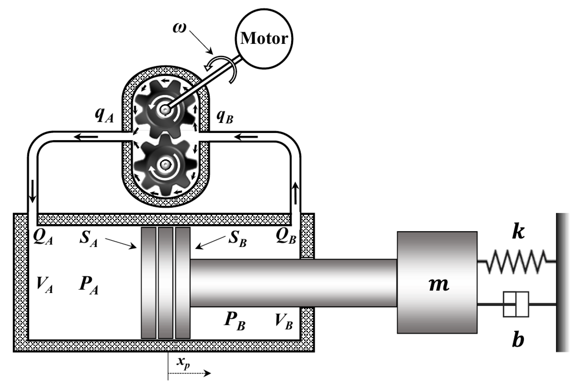
This section introduces the EHA model to be controlled. Figure 1 shows the structure of the single-rod EHA. The chamber volumes and can be expressed as
where is the piston position [m], and are the initial volumes of chambers A and B [m], respectively, including the pipeline, when , is the maximum stroke of the cylinder [m], and are the pressure areas [m]. The flow rate equations of both ports of the actuator can be represented, as follows, when considering the fluid compressibility and continuity principle for the actuator
where and denote the flow in the actuator [m/s], is the effective bulk modulus of the system [N/m], and and are the pressure of both chambers [N/m]. The change of the flow direction and the flow rate adjustment through the port are handled by the electric motor directly connected to the hydraulic pump. In addition, the pressure generated by the continuous supply of flow in the actuator can produce a minute fluid leakage of the pump. Hence, the equations for the fluid leakage of the pump are expressed as
where and are the in-out flow rate of the pump [m/s], is the volumetric capacity of the pump [m/rad], is the rotational speed of the electric motor [rad/s], and is the leakage coefficient of the pump [m/Ns]. The actuator force balance equation of the EHA systems is expressed as
where is the piston velocity [m/s]. m is the total mass of the piston and the load [kg], k is the load spring constant [N/m], and b is the viscous damping coefficient [N/m/s]. We also assume that the conduits that are connected between the actuator ports and the pump ports are very short. The flow rates in (1) through (3) can then be represented as and . The dynamic equation of the EHA systems can be represented as
where and are the volumes of chambers A and B [m], respectively, and . In EHA (5), is physically bounded as
where is a positive constant. The ranges of and are defined as
3. Nonlinear Coordinate Transformation
Let us define a new state and a nonlinear change of coordinates, as
where is the force of the EHA. The relationships between the original and new states are
The dynamics of and are
Control u is defined as . We then obtain the new dynamics of the EHA, as
Equation (11) can be represented as
where
Remark 1.
We now define as the desired position. From (12), and are derived as
where is a positive constant. In , is the part of the desired force for the position tracking, whereas is the part that guarantees the boundedness of .
4. Position Controller
In this section, the design of position controller for tracking the desired state variables for the EHA model (12) is presented.
4.1. Controller Design
The tracking errors are defined as
Remark 2.
The integrator of the position tracking error is defined in order to eliminate the steady-state error due to constant disturbances.
The error dynamics are derived as
The controller u is designed as
where , , , and are control gains. The error dynamics (16) then become
If the control gains , , , and are selected, such that
is Hurwitz, then exponentially converges to zero.
4.2. Stability Analysis of Internal Dynamics
The dynamics of in the new EHA model (12) are internal dynamics as
We will now prove the stability of the internal dynamics. , , and will track , , and , respectively, while using the controller (17). Thus, the zero dynamics are
Theorem 1.
Proof.
Let us define the Lyapunov candidate function as
We have as
where . If is the desired position trajectory for point to point motion, such that , where c is constant, and then . Hense , such that converges to where is constant. If is the desired position trajectory for a repetitive motion, the of the zero dynamics converges to where . Consequently, is globally ultimately bounded in the zero dynamics (21). □
5. Nonlinear Observer Design and Closed-Loop Stability Analysis
In this section, we design the observer in order to estimate the full state. Subsequently, the closed-loop stability is proven using the ISS property.
5.1. Nonlinear Observer Design
The estimated state variable vector is defined as
The dynamics of are designed as
The state estimation error is defined as
The dynamics of are
In the EHA, because is measurable, the estimation error dynamics (27) can be rewritten as
Theorem 2.
Consider the estimation error dynamics (27). If is positive and an affine Lyapunov matrix, exists to satisfy the conditions, such that
then exponentially converges to zero.
Proof.
The problem that analyzes the eigenvalues of (28) for all is equivalent to the robust stability analysis of a linear system with uncertain real parameters [19]. Because , , and are in the sets and , respectively.
where , , , and . The mean values of and with the given sets and , respectively, are presented as
can be rewritten as
With the general EHA parameters and positive , is always Hurwitz. Hence, a symmetric matrix exists, such that . The results in [19] showed that with Hurwitz , if an affine Lyapunov matrix, exists to satisfy condition (29), then is Hurwitz. For given compact sets and , we can then determine the existence of by solving LMI with the MATLAB robust control toolbox. Consequently, exponentially converges to zero. □
Remark 3.
The convergence rate is determined by and the EHA parameters. The output injection parameter will not fully affect the convergence rates of the origin in the estimation error dynamics as the output injection parameter is used in only . However, the convergence rates determined by the EHA parameters in the observer are sufficiently fast when compared with the slow EHA system. Furthermore, with the EHA parameters, exists to satisfy the conditions. Consequently, only a positive is required to guarantee the stability.
5.2. Stability Analysis of Closed-loop System
We define the estimation of as , where
The estimation error of is defined as , where
From (34), , where
In the control input (17), the estimated state variables , , and are used, except for . Hence, the error dynamics (18) become
In (36), and are bounded. Hence, e is ISS stable because is Hurwitz [20]. From Theorem 2, it was proven that exponentially converges to zero. Finally, e converges to zero.
6. Simulations
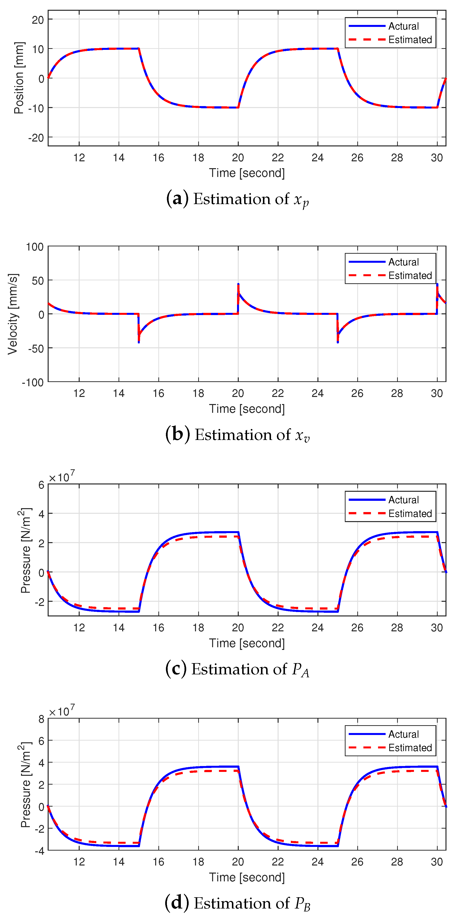
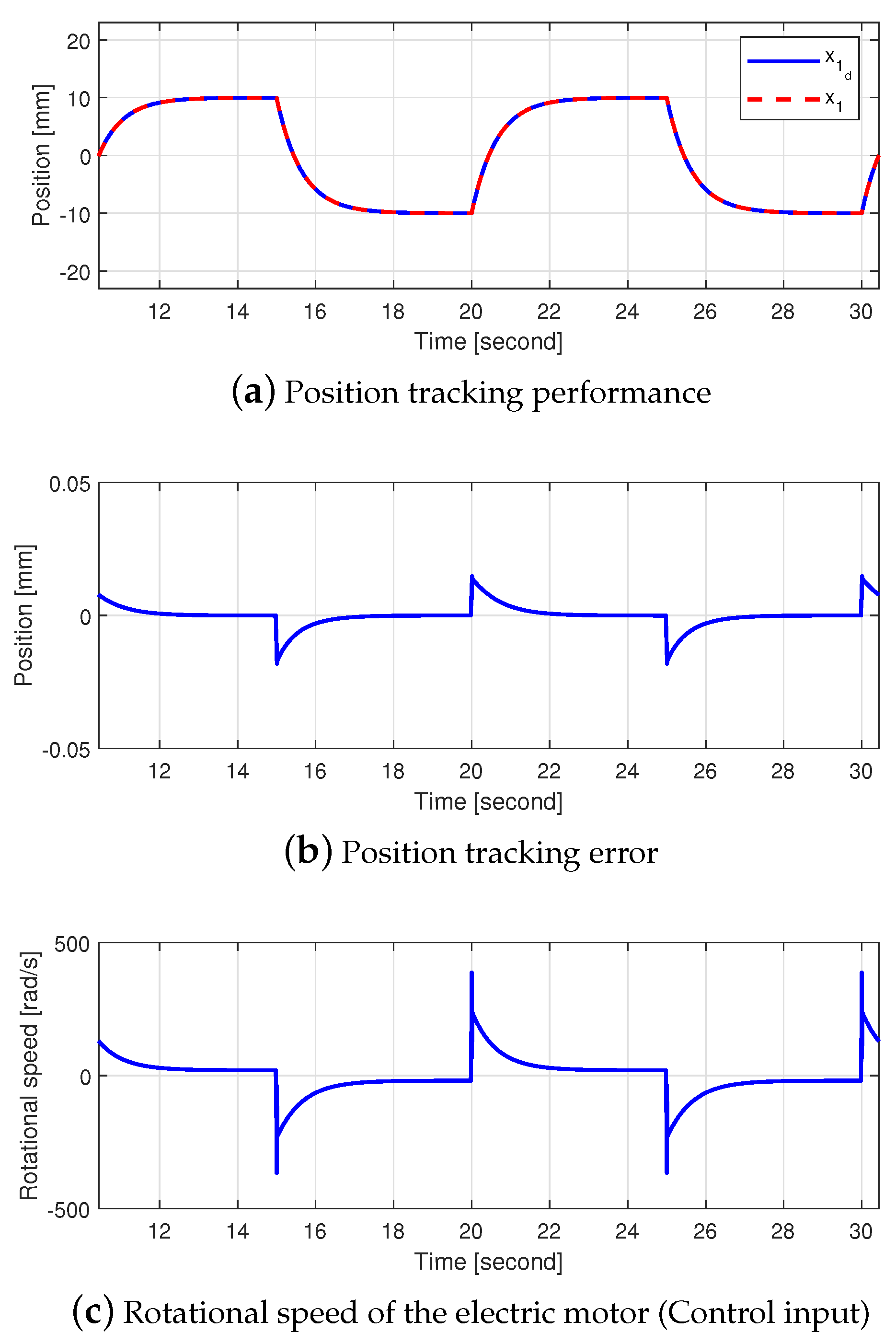
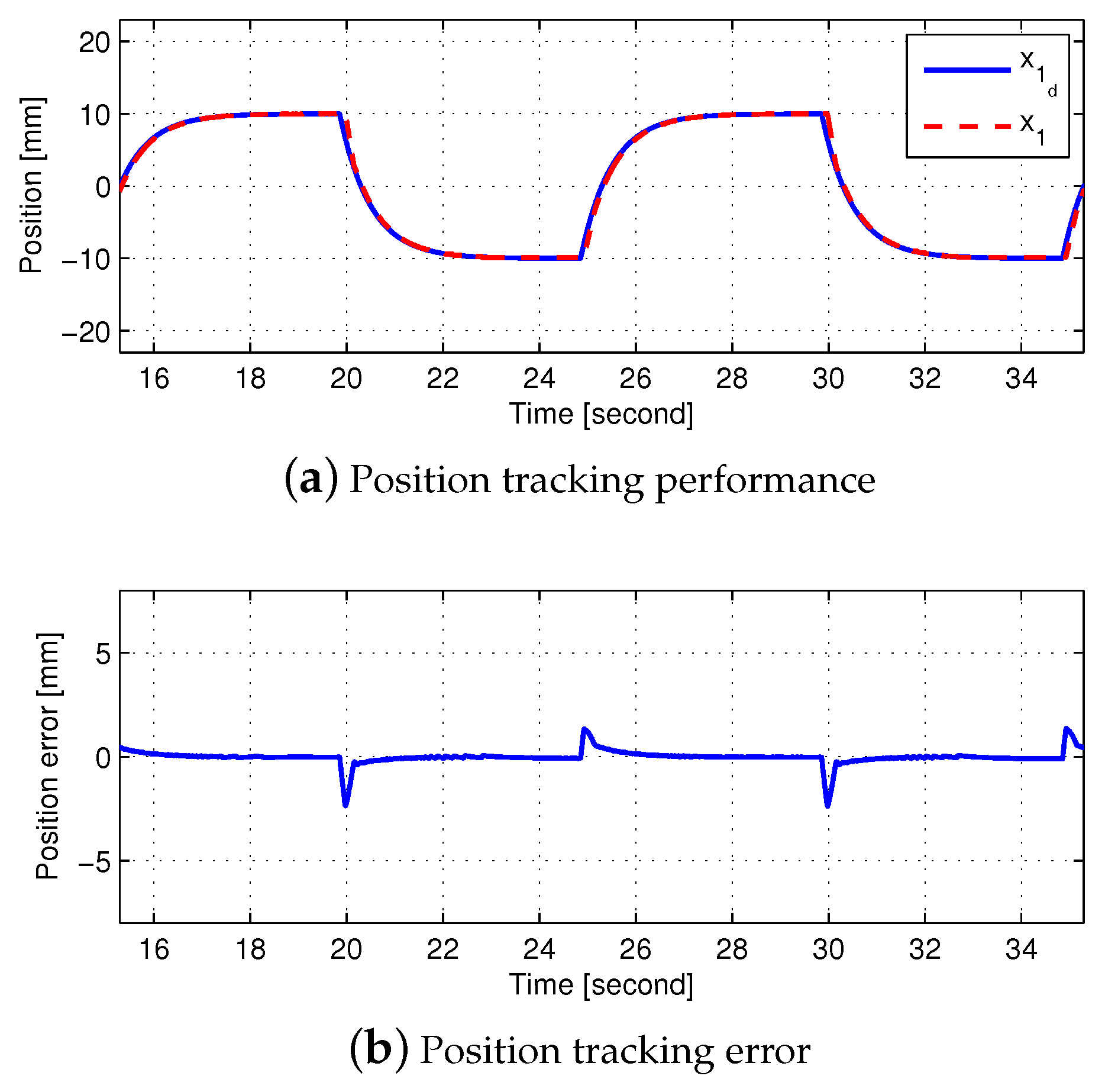
The simulations were conducted in MATLAB/Simulink in order to evaluate the performance of the proposed method. The parameters of the EHA and the control gains listed in Table 1 were used. The load force disturbance was set to 300 Nm. Figure 3 and Figure 4 show the simulation results with the trajectory reference. Figure 3 shows the estimation performance of the proposed method, where the blue and dashed red lines denote the actual and estimated state variables, respectively. The estimated state variables tracked the actual state variables well. A small peak appeared owing to the difference in the initial values of the estimated and actual velocities in the estimation of . Figure 4 shows the position tracking and the control input of the proposed method. The blue and dashed red lines presented in Figure 4a denote the desired and actual positions, respectively. The position tracking error that is shown in Figure 4b is less than . The small peak in the position tracking error appeared owing to the small peak in the estimation of .
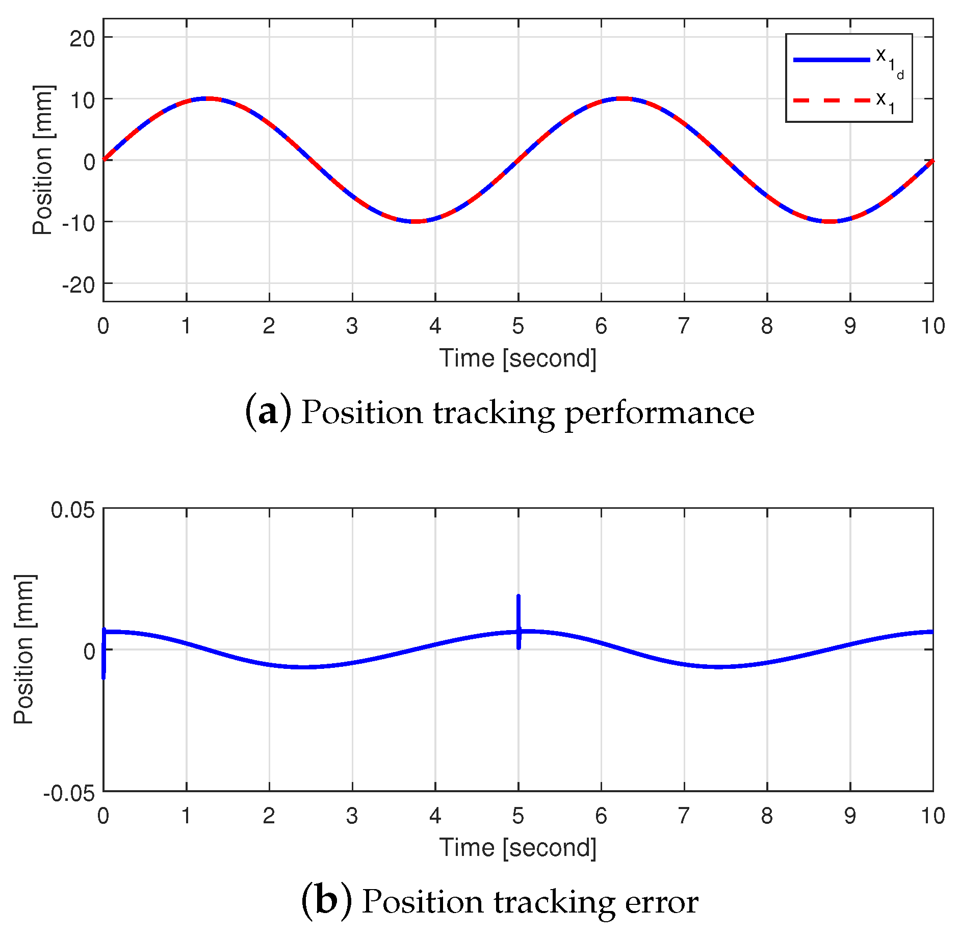
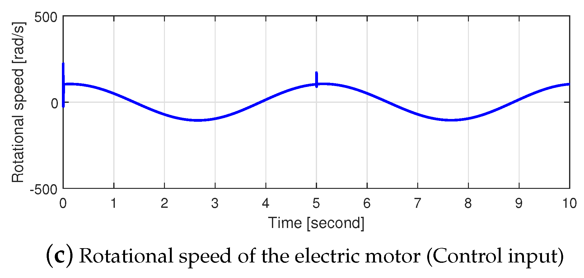
Figure 5 shows the position tracking and the control input of the proposed method with the sinusoidal reference. In this simulation, a step load force disturbance of 300 Nm was injected at 5 s. The blue and dashed red lines presented in Figure 5a denote the desired and actual positions, respectively. At 5 s, a small peak in the position tracking error appeared owing to the step load force disturbance of 300 Nm, but this peak was suppressed by the proposed method. The position tracking error shown in Figure 4b was less than . At 5 s, the small peak in the control input suppressed the step load force disturbance.
7. Experiments
The experiments were executed to evaluate the performance of the proposed method. In the experiments, the proposed method was compared with the proportional-integral (PI) with a feedforward controller used in industrial applications, as follows:
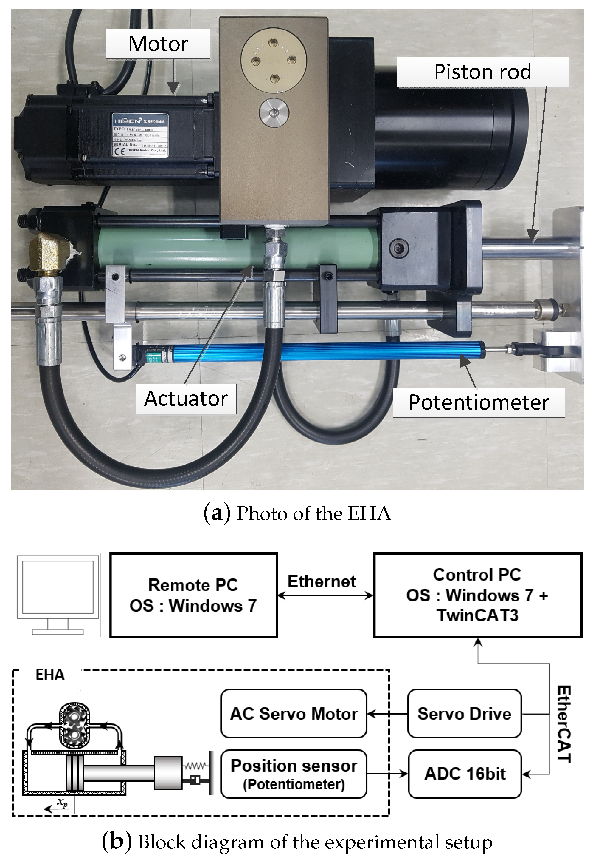
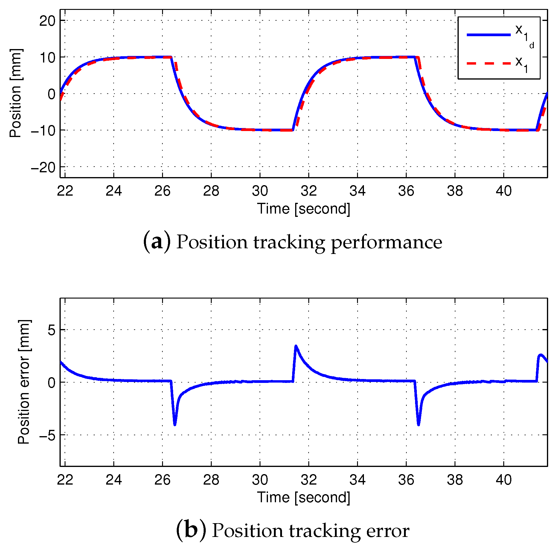
The gains of the PI controller with velocity feedforward were well tuned for tracking the desired position. The same parameters and the load force disturbance were used in both the simulations and experiments. Figure 6 presents the experimental setup. The EHA with the AC servo motor designed by KCC Co., Ltd. was used. The effective stroke of the piston range was ±0.025 m. Only a potentiometer was used as the sensor to measure the position. For the experiments, the control algorithms (i.e., the proposed method and the PI controller with velocity feedforward) that were coded in C by an S-function were used in realtime operating systems. The derivatives in the control law formulation were calculated using the Tustin method. A sampling rate of 1 kHz and 16-bit A/D and 16-bit D/A converters were also used. Figure 7 and Figure 8 present the position tracking performances of both methods. In the PI controller with the velocity feedforward, the peaks of the position tracking errors appeared due to the static friction whenever the direction of motion was changed. Furthermore, relatively significant lag also appeared. On the contrary, the peaking in the transient responses was suppressed by the proposed method. In the proposed method, the position tracking error rapidly converged to zero when compared with the PI controller with the velocity feedforward. Meanwhile, the influence of friction was insignificant in the proposed method. The use of the proposed method resulted in decreasing the phase lag. The position tracking error of the proposed method was less than that of the PI with velocity feedforward. Hence, the position tracking performances in both the transient and steady-state responses were improved by the proposed method.
8. Conclusions
The observer based nonlinear position control with nonlinear coordinate transformation using only position measurement was proposed in order to improve the position tracking performance in single-rod EHAs. The proposed method consisted of a position controller and an observer. The nonlinear coordinate transform was presented to design the simple position controller. The position controller was designed to track the desired state variables, while the observer was proposed to estimate the full state using only the position feedback. The performance of the proposed method was validated via simulations and experiments. It was shown that the proposed method reduced the position tracking errors in both the transient and steady-state responses. Consequently, the proposed method can improve the the position tracking performance using only the position measurement in both the transient and steady-state responses.
Author Contributions
Both authors contributed equally to this work. The original draft was written by W.K. and review & editing were conducted by D.W. All authors have read and agreed to the published version of the manuscript.
Funding
This research was funded by the Korea Institute of Industrial Technology as “Development of industrial robot and postprocessing robot application technology for Ppuri industry (kitech JH200006)” project.
Conflicts of Interest
The authors declare that they have no conflicts of interest.
References
- Merrit, H.E. Hydraulic Control System; Wiley and Sons: New York, NY, USA, 1967. [Google Scholar]
- Grabbel, J.; Ivantysynova, M. An investigation of swash plate control concepts for displacement controlled actuators. Int. J. Fluid Power 2005, 6, 19–36. [Google Scholar] [CrossRef]
- Chen, T.; Wu, Y. An optimal variable structure control with integral compensation for electrohydraulic position servo control systems. IEEE Trans. Ind. Electron. 1992, 39, 460–463. [Google Scholar] [CrossRef]
- Guan, C.; Pan, S. Adaptive sliding mode control of electro-hydraulic system with nonlinear unknown parameters. Control Eng. Prac. 2008, 16, 1275–1284. [Google Scholar] [CrossRef]
- Tsao, T.-C.; Tomizuka, M. Robust adaptive and repetitive digital tracking control and application to a hydraulic servo for noncircular machining. J. Dyn. Syst. Meas. Control 1994, 116, 24–32. [Google Scholar] [CrossRef]
- Hahn, H.; Piepenbrink, A.; Leimbach, K.-D. Input/output linearization control of an electro servo-hydraulic actuator. In Proceedings of the 1994 Conference on Control Applications, Glasgow, UK, 24–26 August 1994; pp. 995–1000. [Google Scholar]
- Seo, J.; Venugopala, R.; Kenné, J.-P. Feedback linearization based control of a rotational hydraulic drive. Control Eng. Pract. 2007, 15, 1495–1507. [Google Scholar] [CrossRef]
- Kim, W.; Shin, D.; Won, D.; Chung, C.C. Disturbance observer based position tracking controller in the presence of biased sinusoidal disturbance for electro-hydraulic actuators. IEEE Trans. Control Syst. Technol. 2013, 21, 2290–2298. [Google Scholar] [CrossRef]
- Alleyne, A.; Liu, R. A simplified approach to force control for electro-hydraulic systems. Control Eng. Pract. 2000, 8, 1347–1356. [Google Scholar] [CrossRef]
- Yao, B.; Bu, F.; Reedy, J.; Chiu, G.T.C. Adaptive robust motion control of single-rod hydraulic actuators: Theory and experiments. IEEE/ASME Trans. Mechatron. 2000, 5, 79–91. [Google Scholar]
- Kaddissi, C.; Kenné, J.-P.; Saad, M. Identification and real-time control of an electrohydraulic servo system based on nonlinear backstepping. IEEE/ASME Trans. Mechatron. 2007, 12, 12–22. [Google Scholar] [CrossRef]
- Kaddissi, C.; Kennè, J.-P.; Saad, M. Indirect adaptive control of an electrohydraulic servo system based on nonlinear backstepping. IEEE/ASME Trans. Mechatron. 2012, 16, 1171–1177. [Google Scholar] [CrossRef]
- Kim, W.; Won, D.; Tomizuka, M. Flatness-based nonlinear control for position tracking of electrohydraulic systems. IEEE/ASME Trans. Mechatron. 2015, 20, 197–206. [Google Scholar] [CrossRef]
- Kim, H.M.; Park, S.H.; Lee, J.M.; Kim, J.S. A robust control of electro hydrostatic actuator using the adaptive backstepping scheme and fuzzy neural networks. Int. J. Precis. Eng. Manuf. 2010, 11, 227–236. [Google Scholar] [CrossRef]
- Wang, L.; Book, W.J.; Huggins, J.D. Application of singular perturbation theory to hydraulic pump controlled systems. IEEE/ASME Trans. Mechatron. 2012, 17, 251–259. [Google Scholar] [CrossRef]
- Kim, W.; Won, D.; Shin, D.; Chung, C.C. Output feedback nonlinear control for electro-hydraulic systems. Mechatronics 2012, 22, 766–777. [Google Scholar] [CrossRef]
- Guo, Q.; Zhang, Y.; Celler, B.G.; Su, S.W. Backstepping control of electro-hydraulic system based on extended-state-observer with plant dynamics largely unknown. IEEE Trans. Ind. Electron. 2016, 63, 6909–6920. [Google Scholar] [CrossRef]
- Won, D.; Kim, W.; Tomizuka, M. High gain observer based integral sliding mode control for position tracking of electro-hydraulic systems. IEEE/ASME Trans. Mechatron. 2017, 22, 2695–2704. [Google Scholar] [CrossRef]
- Gahinet, P.; Apkarian, P.; Chilali, M. Affine parameter-dependent Lyapunov functions and real parametric uncertainty. IEEE Trans. Autom. Control 1996, 41, 436–442. [Google Scholar] [CrossRef]
- Khalil, H. Nonlinear Systems, 3rd ed.; Prentice-Hall: Upper Saddle River, NJ, USA, 2002. [Google Scholar]
- Yao, B.; Bu, F.P.; Chiu, G.T.C. Nonlinear adaptive robust control of electro-hydraulic servo system with discontinuous projection. In Proceedings of the 37th IEEE Conference on Decision and Control, Tampa, FL, USA, 16–18 December 1998; pp. 2265–2270. [Google Scholar]
- Do, K.D.; Pan, J. Boundary control of transverse motion of marine risers with actuator dynamics. J. Sound Vib. 2008, 318, 768–791. [Google Scholar] [CrossRef]
Figure 1.
Structure of the single-rod electro-hydrostatic actuator.

Figure 2.
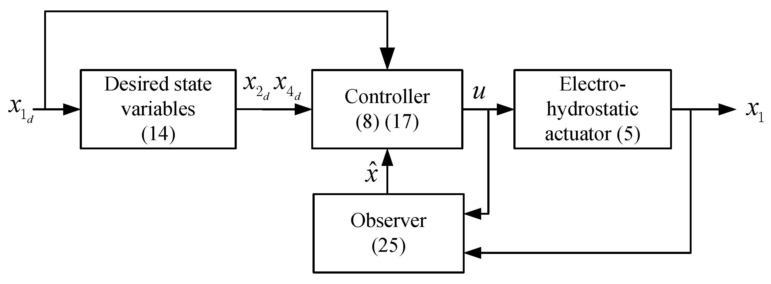
Lock diagram of the controller structure.

Figure 3.
Estimation results of the proposed state observer in simulations with the trajectory reference.
Figure 3.
Estimation results of the proposed state observer in simulations with the trajectory reference.

Figure 4.
Position tracking performance of the proposed method in simulations with the trajectory reference.
Figure 4.
Position tracking performance of the proposed method in simulations with the trajectory reference.

Figure 5.
Position tracking performance of the proposed method in simulations with the sinusoidal reference.
Figure 5.
Position tracking performance of the proposed method in simulations with the sinusoidal reference.


Figure 6.
Experimental setup of the EHS system.

Figure 7.
Position tracking performance of the PI and feedforward controller in experiments.

Figure 8.
Position tracking performance of the proposed method in experiments.


Table 1.
Parameters.
| Parameter | Value | Parameter | Value |
|---|---|---|---|
| k | 4000 | b | 100 |
| m | 80 | ||
| 3800 | 100 |
© 2020 by the authors. Licensee MDPI, Basel, Switzerland. This article is an open access article distributed under the terms and conditions of the Creative Commons Attribution (CC BY) license (http://creativecommons.org/licenses/by/4.0/).
Share and Cite
MDPI and ACS Style
Kim, W.; Won, D. Nonlinear Position Control with Nonlinear Coordinate Transformation Using Only Position Measurement for Single-Rod Electro-Hydrostatic Actuator. Mathematics 2020, 8, 1273. https://doi.org/10.3390/math8081273
AMA Style
Kim W, Won D. Nonlinear Position Control with Nonlinear Coordinate Transformation Using Only Position Measurement for Single-Rod Electro-Hydrostatic Actuator. Mathematics. 2020; 8(8):1273. https://doi.org/10.3390/math8081273
Chicago/Turabian StyleKim, Wonhee, and Daehee Won. 2020. "Nonlinear Position Control with Nonlinear Coordinate Transformation Using Only Position Measurement for Single-Rod Electro-Hydrostatic Actuator" Mathematics 8, no. 8: 1273. https://doi.org/10.3390/math8081273
Note that from the first issue of 2016, this journal uses article numbers instead of page numbers. See further details here.