Article

Experimental Determination of Non-Linear Roll Damping of an FPSO Pure Roll Coupled with Liquid Sloshing in Two-Row Tanks

1
Department of Civil, Environmental and Ocean Engineering, Stevens Institute of Technology, Castle Point on Hudson, Hoboken, NJ 07030, USA
2
Department of Ocean Engineering, Texas A & M University, College Station, TX 77843, USA
*
Author to whom correspondence should be addressed.
J. Mar. Sci. Eng. 2020, 8(8), 582; https://doi.org/10.3390/jmse8080582
Submission received: 16 June 2020 / Revised: 24 July 2020 / Accepted: 24 July 2020 / Published: 3 August 2020
(This article belongs to the Special Issue Ship Dynamics for Performance Based Design and Risk Averse Operations)

Abstract

:
Wave excited roll motion poses danger for moored offshore vessels such as Floating Production Storage and Offloading (FPSO) because they cannot divert to avoid bad weather. Furthermore, slack cargo tanks are almost always present in FPSOs by design. These pose an increased risk of roll instability due to the presence of free surfaces. The most common method of determining roll damping is roll decay tests, yet very few test have been performed with liquid cargo, and most liquid cargo experiments use tanks that span the entire width of the vessel; which is seldom the case for full scale FPSO vessels during normal operations. This paper presents a series of roll decay test carried out on a FPSO model with two two-row-prismatic tanks with different filling levels. To directly investigate the coupling between the liquid sloshing and the vessel motion, without modifying the damping, tests were performed at a constant draft. The equivalent linear roll damping coefficients consisting of linear, quadratic and cubic damping terms are analyzed for each loading condition using four established methods, the Quasi-linear method, Froude Energy method, Averaging method and the Perturbation method. The results show that the cubic damping term is paramount for FPSOs and at low filling levels, were the FPSO is more damped. Recommendations regarding the applicability of the methods, their accuracy and computational effort is given and the effect of the liquid motion on the vessel motion is discussed.

1. Introduction

Roll motion is the most dangerous motion amongst the six degrees of freedom because it can lead to capsizing [1,2], causes crew discomfort, and thus reduce the vessel’s efficiency [3]. Roll motion is especially critical for offshore floating vessels such as Floating Production Storage and Offloading (FPSO) units because they are expected to operate at a location for extended duration and as such cannot avoid severe weather conditions. In addition, FPSOs experience continuous cargo loading and offloading [4], hence slack tanks cannot be avoided. Oscillations in slack cargo tanks can effect the roll motion characteristics of the vessel, it is therefore important to consider the free surface effect on roll damping [5].
Damping effects can be classified into linear and nonlinear components. Linear damping does not consider the viscosity of the liquid and it is described using linear radiation/diffraction theory [6]. Nonlinear damping includes the effects of liquid viscosity and appendages [6,7]. The vessel’s roll damping can be described as linear for vessels with small roll amplitudes [8] but linear models are insufficient for vessels with large roll amplitudes, therefore, nonlinearities need to be accounted for when the roll amplitude is large enough to capsize the vessel [9]. Nonlinearities are further important when considering the effect of bilge keels [10] or liquid cargo motion [5].
Froude [11] was the earliest to predict nonlinear roll motion effects on floating vessels. Subsequently, Ikeda et al. [12] developed an empirical method that divided roll damping into five components (skin friction on the hull, eddy making, wave, lift and appendages). This empirical method provided low accuracy for damping at large angles, cannot handle attributes of complex flows [13] and are only applicable at the design stage [14]. Beyond design stage, excited roll motion, forced roll motion and the free roll decay test [15] are three methods for determining the nonlinear roll motion. These three methods can be done by experiment or by Computational Fluid Dynamics (CFD).
For forced roll motion, the model is rotated with the aid of a mechanical device and it is maintained in a fixed axis [15,16]. Kinnas [17] simulated a FPSO with and without bilge keels in harmonic forced motion and he observed a linear relationship between roll moment and roll amplitude in inviscid flow and a nonlinear relationship between the roll moment and roll angle in viscous flow. Thiagarajan et al. [18] did forced roll motion studies numerically and experimentally for an FPSO and concluded that the amplitude of the damping was influenced by the roll angular velocity and the bilge keel widths.
Using the excited roll motion method, the model is freely floating and it is excited by regular beam waves or an internal mechanical device such as a gyro roll exciter or a contra-rotating mass or an internal lateral shifting mass [14]. Blume [19] obtained roll damping coefficients using this method and he showed that roll damping coefficient was dependent on the maximum roll angle, metacentric height and heel angle of the vessel but Blume’s method had long measurement time. Using same method, Handschel and Maksoud [20] improved on Blumes work by reducing the measuring time, improving the estimation accuracy of roll damping coefficient over a wide frequency range and provided possibilities of determining roll damping with nonlinear stability moment curve. Wasserman et al. [21] compared experimental and numerical results obtained from excited roll motion and free roll decay test and concluded that the excited roll motion was superior to the roll decay test for larger damping values.
Despite the findings by Wasserman et al. [21], free roll decay test is the most widely used method [5,22,23,24,25,26,27] because it is the recommended technique by the International Maritime Organization (IMO) [28]. There are five methods to determine the damping coefficients for the vessel roll motion from roll decay test [29]: Quasi-linear method, Froude Energy method, Roberts Energy method, Averaging method and the Perturbation method.
The Quasi-linear method is the simplest method because the equivalent linearised damping coefficient with respect to the roll angle amplitude can be directly obtained without the need for any curve fitting. It further, permits aggregating data from different decay tests as long as it is the same loading condition [14], this is beneficial for vessels with higher dampening since they will experience fewer oscillations before reaching steady state. The roll decrement is calculated from successive peaks or successive troughs or the double amplitudes of the roll decay curve (see Figure 1) [21]. This method is sometimes referred to as the logarithmic decrement method [30]. Though widely used [5,14,28,30,31,32], this method can be highly inconsistent because it sometimes shows poor correlation between the roll decrements and the roll angle amplitudes, leading to a incorrect damping coefficient [33].
The two main energy methods based on energy conservation are: Froude and Roberts [21,29]. Froude energy method assumes that for each half cycle, the energy lost by damping is equal to the work done by the hydrostatic restoring moment that reduces the roll amplitude. Roberts energy method [34] equates roll damping to an energy loss function. Froude energy method does not necessarily require a curve fitting for the roll angle series, it is weakly sensitive to shift in the origin of roll angle measurement in the vertical and horizontal direction due to roll period, errors in righting arm estimation, and roll amplitude definition. Roberts method on the other hand requires curve fitting and it is strongly sensitive to a shift of the origin of roll angle measurement [21]. A comparative studies have been carried out to compare the Quasi-linear and Energy methods and they agree that the Quasi-linear method is more susceptible to errors [29] and the energy methods are suitable for larger amplitudes based on curve fitting of the energy envelop [15,21]. Since both Roberts and Froude method are both based on conservation of energy, only Froude energy method will be treated in this paper.
The Averaging method by Kryloff and Bgoliuboff [35] assumes the profile of the roll decay is sinusoidal and the rate of change of the amplitude and phase is constant at their average values for each cycle, that make this method to be more applicable for light damped systems [35]. It is more complex than the other methods because it produces a complex expression for the decay envelop. Though it is reliable, it is sensitive to the first peak of the decay motion hence, a distortion in the first peak of the decay would affect results obtained by this method [29].
The Perturbation method assumes that the nonlinear damping terms are small compared to the linear damping terms. This assumption permits the solution of the roll motion to be treated as a linear motion with some perturbations. This makes this method more complicated than the other methods as the roll decay angle amplitude envelop needs to be fitted with a higher order nonlinear equation with three unknown variables [29].
The damping coefficient may be dependant on the chosen analyzing method [28] or it may be affected by the different definitions of the average roll amplitude ( ϕ m ) (Equations (11) and (12)) [21]. Other factors that can affect the damping coefficients obtained are the estimation of the righting moment (GZ) of the vessel [15]. Therefore, choosing which method, mathematical model and the average roll amplitude to use to determine the damping coefficients is challenging, and more research on the topic is needed.
This paper investigates the equivalent linear damping coefficients obtained using four methods and two mathematical models for roll damping from a roll decay test of a model scale FPSO. A series of roll decay test on the FPSO model with two two-row prismatic tanks with different filling levels was carried out at the Davidson Laboratory of Stevens Institute of Technology. The test were performed at constant draft, constant displacement and only roll motion was applied. The obtained damping is dependant on the chosen analyzing method, by comparing the effect of the number of terms included in the curve fit needed to obtain the dampening coefficient, guidance regarding method selection can be provided. The effect of the liquid motion on the vessel motion and the effect of change in draft are further discussed.

2. Theoretical Background

The model was free to roll, but fixed in all other degrees of freedom (DOFs), the dynamic behaviour of the vessel is therefore described by the single degree of freedom (DOF) equation:
( I + A ) ϕ ¨ + B ( ϕ ) ϕ ˙ + C ( ϕ ) ϕ = F ( t )
where I is the roll mass moment of inertia (Kg m 2 ), A is the added mass moment inertia (Kg m 2 ), B ( ϕ ) is the roll damping coefficient (Nm.s), C ( ϕ ) is the restoring stiffness coefficient (Nm) and F is the time dependent forcing moment which is zero for calm water tests. ϕ , ϕ ˙ and ϕ ¨ are the roll angle, angular velocity and angular acceleration respectively. C = ρ g G Z where ρ is the model mass (Kg) and G Z is the angle dependent restoring lever (m) [36]. The normalised form of the roll motion is:
ϕ ¨ + b ( ϕ ) ϕ ˙ + c ( ϕ ) ϕ = f ( t )
where b ( ϕ ) is the roll damping coefficient per mass moment of inertia = B ( ϕ ) ( I + A ) , c ( ϕ ) is the roll stiffness coefficient per unit mass moment of inertia = C ( ϕ ) ( I + A ) and f ( t ) is the applied moment per mass moment of inertia = F ( t ) ( I + A ) .
The nonlinear damping moment per mass moment of inertia b ( ϕ ) can be expressed by a series expansion consisting of a linear term and higher order nonlinear terms, as a function of ϕ and ϕ ˙ [37]:
b ( ϕ ) ϕ ˙ T o t a l d a m p i n g = b 1 ϕ ˙ L i n e a r d a m p i n g t e r m + b 2 | ϕ ˙ | ϕ Q u a d r a t i c d a m p i n g t e r m + b 3 ϕ ˙ 3 C u b i c d a m p i n g t e r m + O ( ϕ 4 ) H i g h e r 4 t h o r d e r t e r m s
Inserting Equation (3) in Equation (2) for a calm water roll decay test, where f ( t ) = 0 , the normalised equation of motion for the vessel becomes:
ϕ ¨ + b 1 ϕ ˙ + b 2 | ϕ ˙ | ϕ ˙ + b 3 ϕ ˙ 3 + c ( ϕ ) ϕ = 0
Equation (4) is an accurate mathematical model of dynamic ship rolling in calm water, since it includes the effects of the resistance due to the linear damping coefficient b 1 and nonlinear damping coefficients b 2 and b 3 . However, this nonlinear equation is rarely solved [7], since it requires iterative numerical ODE solvers to overcome the non-linearity in the equation represented by terms | ϕ ˙ | ϕ ˙ and ϕ ˙ 3 . Hence using a linearized equivalent equation is beneficial. In the linearized form the total damping coefficient b ( ϕ ) is replaced by an equivalent linear damping coefficient b e ( ϕ a ) [7,29] which is dependent on the vessel roll angle amplitude and the roll period. The linear, quadratic and cubic damping coefficients are also kept constant in the equivalent linear damping. The linearized one DOF equation of motion with equivalent damping coefficient is:
ϕ ¨ + b e ( ϕ a ) ϕ ˙ + c e ( ϕ a ) ϕ = 0
where c e ( ϕ a ) is the amplitude dependent stiffness and ϕ a is the roll angle amplitude at certain time. The relationship between the total damping and the equivalent linear damping is:
b ( ϕ ) = b e ( ϕ a )
b e ( ϕ a ) = b 1 + 8 3 π ω d ϕ a b 2 + 3 4 ω d 2 ϕ a 2 b 3

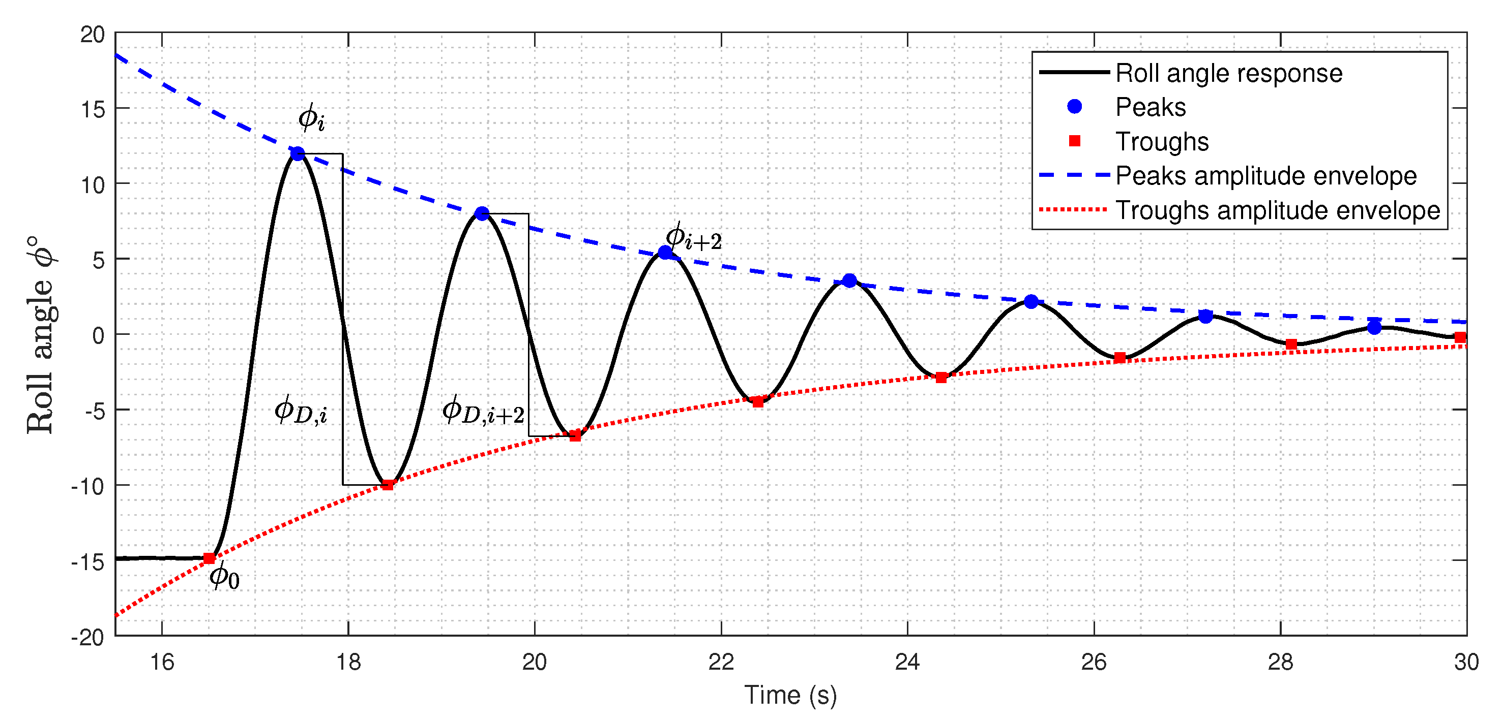
2.1. Quasi-Linear Method (Logarithmic Decrement)

The Quasi-linear or the Logarithmic decrement method is considered to be the simplest technique to directly compute the equivalent linear damping coefficient b e with respect to the roll angle amplitude obtained through roll decay tests [29]. The transient roll angle ϕ ( t ) is assumed to be a sinusoidal motion with decaying amplitude as shown in Equation (8), where ϕ 0 is the initial roll angle amplitude and ϕ a ( t ) is the decaying amplitudes for peaks or troughs as shown in Figure 1 and Equation (9).
By applying Equation (9) for two successive peaks i and i + 1 (or troughs), of the decaying envelope, the logarithmic decay can be determined (Equation (10)) and then the equivalent linear damping coefficient (Equation (11)).
When measuring the roll angle, a measurement offset may occur causing irregularity of peaks and troughs amplitudes envelopes leading to different predictions of the damping coefficient by peak based or trough based envelopes. The double amplitude based logarithmic decay technique [21] is used to compensate this possible offset, instead of analysing the peaks’ envelope and the troughs’ envelope separately, the absolute difference between each peak and following trough is considered as shown in Figure 1, and the equivalent linear damping coefficient is obtained using Equation (12) [36]. Figure 2 shows the equivalent linear damping coefficient b e (12) as a function of the average roll angle amplitude ϕ m , the plot is a combination of four roll decay tests with different initial roll angles for loading condition 8 (see Section 3.3).
ϕ ( t ) = ϕ 0 e b e t 2 cos ( ω d t )
ϕ a ( t ) = ϕ 0 e b e t 2
ϕ i + 1 ϕ i = e b e 2 ( t i + 1 t i )
b e ( ϕ m ) = ω d π ln ϕ i ϕ i + 1 , f o r ϕ m = ϕ i + ϕ i + 1 2
b e ( ϕ m ) = ω d π ln ϕ D , i ϕ D , i + 2 , f o r ϕ m = ϕ D , i + ϕ D , i + 2 4

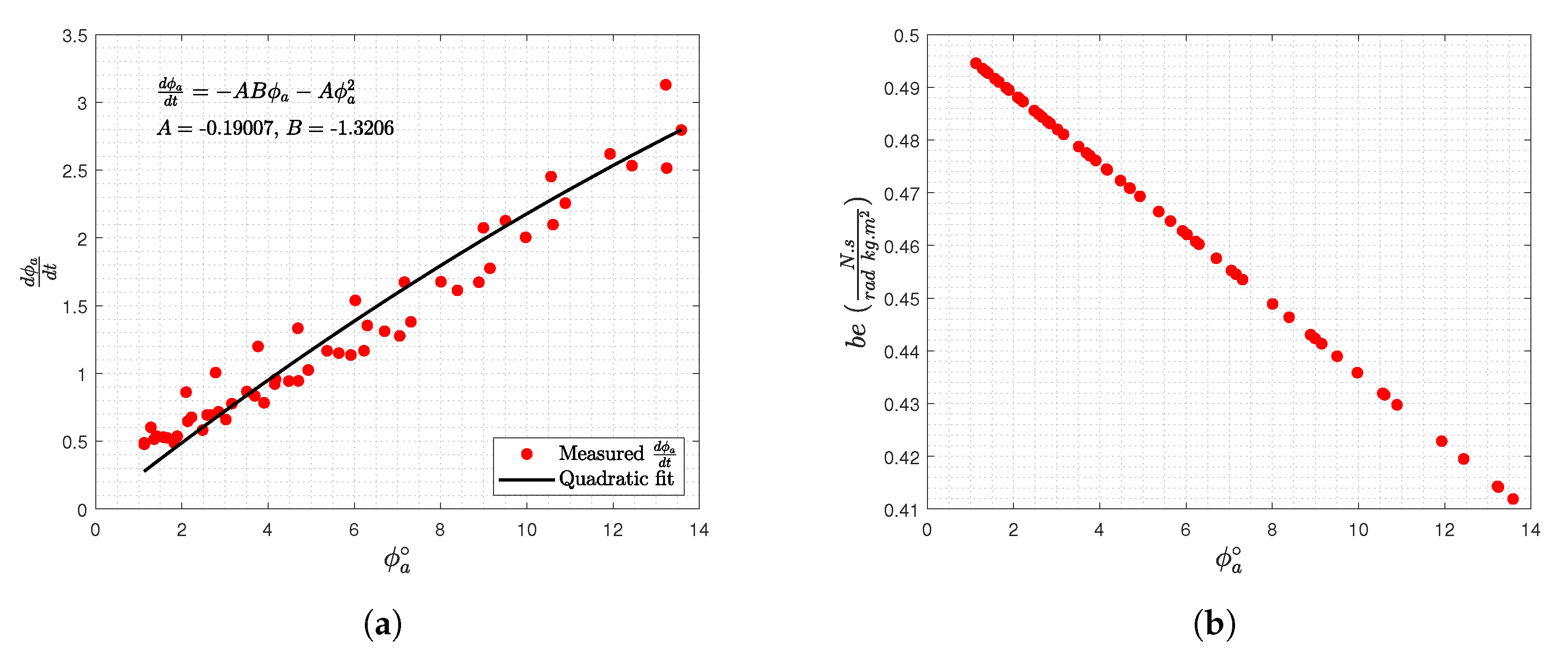
2.2. Froude Energy Method

Froude energy method [7,36] is based on the assumption that the energy lost due to the damping E D 1 2 in a half cycle is equivalent to the hydrostatic stiffness restoring energy applied by the restoring lever arm E r 1 2 :
E D 1 2 = E r 1 2
The energy lost by damping in a half cycle and restored by stiffness are calculated by assuming that the motion is sinusoidal through each quarter cycle as shown in Equation (14), compared with the Quasi-linear method that assumes that the motion is sinusoidal with an exponential decaying term (Equation (8)).
ϕ = ϕ i s i n ( w d t )
ϕ 1 is the amplitude of the roll motion in the first quarter cycle quarter ϕ 1 ϕ 0 , ϕ 2 is the amplitude of the roll motion over the second quarter cycle 0 ϕ ϕ 2 as shown in Figure 3, ω d is the natural damped angular frequency. Equation (14) is only valid for a quarter cycle, hence the half cycled energy terms must be calculated by the summation of energy terms in each cycle quarter as:
E D 1 1 4 + E D 2 1 4 = E r 1 1 4 + E r 2 1 4
The energy dissipation including linear, quadratic and cubic damping in a quarter cycle is described by Equation (16), hence the total energy dissipation during the half cycle between amplitudes ϕ 1 and ϕ 2 can be described using Equation (17).
E D i 1 4 = 0 π 2 w d ( b 1 ϕ ˙ i 2 + b 2 | ϕ ˙ i | ϕ ˙ i 3 + b 3 ϕ ˙ i 4 ) · d t
E D 1 2 = 0 π 2 w d ( b 1 ( ϕ ˙ 1 2 + ϕ ˙ 2 2 ) + b 2 ( | ϕ ˙ 1 + ϕ ˙ 2 | ( ϕ ˙ 1 3 + ϕ ˙ 2 3 ) ) + b 3 ( ϕ ˙ 1 4 + ϕ ˙ 2 4 ) ) · d t
Integrating Equation (17) gives Equation (18) which is the energy dissipated in the half cycle from ϕ 1 to ϕ 2 . For ϕ 1 ϕ 2 and ϕ a = ( ϕ 1 + ϕ 2 2 ) the total energy dissipation can be simplified as shown in Equation (19).
E D 1 2 = 1 4 π b 1 ω d ( ϕ 1 2 + ϕ 1 2 ) + 2 3 b 2 ω d 2 ( ϕ 1 3 + ϕ 2 3 ) + 3 16 b 3 π ω d 3 ( ϕ 1 4 + ϕ 2 4 )
E D 1 2 = 1 2 π b 1 ω d ϕ a 2 + 4 3 b 2 ω d 2 ϕ a 3 + 3 8 b 3 ω d 3 π ϕ a 4
The energy done by the restoring moment lever arm during the half cycle between ϕ 1 and ϕ 2 is described by Equation (20). By averaging the the successive amplitudes the restoring energy can be represented using Equation (21), where ϕ a = ϕ 1 + ϕ 2 2 , c = ω d 2 and d ϕ d r = ϕ 1 ϕ 2 .
E r 1 2 = ϕ 2 ϕ 1 c ϕ d ϕ = c 2 [ ϕ 1 2 ϕ 2 2 ]
E r 1 2 = ω d 2 ϕ a d ϕ d r
By equating Equations (19) and (21) the decrease of amplitudes per half cycle d ϕ a d r can be represented by a third order polynomial as shown in Equation (22). This equation can be solved by determining the decay extinction coefficients: a , b and c. They can be determined by a third order polynomial fit or second order polynomial fit if only the linear (a) and quadratic ( b ) damping are considered.
d ϕ a d r = π b 1 2 ω d ϕ a a ϕ a + 4 3 b 2 ϕ a 2 b ϕ a 2 + 3 8 ω d π b 3 ϕ a 3 c ϕ a 3
a e = a + b ϕ a + c ϕ a 2 = π b e 2 ω d
Figure 4 and Figure 5 shows two examples of the Froude energy method used to determine the equivalent damping coefficient per mass moment of inertia b e (Equation (23)). In Figure 4a the decrease in half cycle amplitudes is plotted as a function of the mean peak roll angle amplitude then fitted with a quadratic polynomial to estimate the first two coefficients a and b (see Equation (22)), then the equivalent damping coefficient is determined for the range of roll peak amplitudes using Equation (23), see Figure 4b. In Figure 5a the results are fitted by a third order degree polynomial to compute the three extinction coefficients a , b and c, the equivalent damping coefficient including the cubic damping term are plotted in Figure 5b. By comparing Figure 4b and Figure 5b It is obvious that after including the cubic damping term, the behaviour of the equivalent damping with respect to the roll angle peak amplitude is changed as an inflection point appears near 10 after which the the damping is increasing.

2.3. Averaging Method

The Averaging method developed by Kryloff and Bgoliuboff [29,35] is designed for lightly damped systems. The Froude energy method assumes a sinusoidal motion of only half of the cycle, the Averaging method on the other hand assumes the roll angle to be in a sinusoidal form for the whole cycle, with a slight amplitude decay with respect to the time, as expressed in Equation (25). By inserting ϕ ( t ) (Equation (25)) in the equation of motion (24) and integrating over the whole cycle [35], an expression for the rate change of amplitude d ϕ a d t is generated as shown in Equations (26) and (27). Equation (27) represents the relation between the amplitude rate change d ϕ a d t with the roll angle amplitude ϕ a by a second order equation which is fitted by the nonlinear least square algorithm to evaluate the linear and nonlinear damping coefficients b 1 and b 2 (Equation (28)) as shown in Figure 6a. Figure 6b shows the estimated equivalent linear damping coefficient per mass moment of inertia b e , Equation (28).
ϕ ¨ + b 1 ϕ ˙ + b 2 ϕ ˙ | ϕ ˙ | + c ϕ = 0
ϕ ( t ) = ϕ a ( t ) cos ( ψ ) , ψ = ω d t + θ
d ϕ a d t = 1 2 π ω d 0 2 π b 1 ϕ a ω d c o s 2 ( ψ ) + b 2 ( ϕ a ω d ) 2 | c o s ( ψ ) | c o s 2 ( ψ ) d ( ψ )
d ϕ a d t = 4 b 2 ω d 3 π 3 π b 1 8 b 2 ω d ϕ a A B ϕ a 4 b 2 ω d 3 π ϕ a 2 A ϕ a 2
b e = b 1 + 8 3 π b 2 ϕ a ω d

2.4. Perturbation Method

The Perturbation method is considered the most complicated method for analyzing roll decay test data [29], because the roll decay angle amplitude envelope (Figure 7a) is fitted with a high order nonlinear equation with three unknown variables.
The Perturbation method assumes the nonlinear damping coefficients are small compared to the linear damping coefficient. The motion is described using Equation (29), where ϵ is the perturbation expansion parameter. This equation is assumed to have a solution represented by a power series of ϵ , Equation (30). By inserting the zero, first and second order expansions (Equation (30)) in (29), a new equation of motion is obtained for each expansion. The equations are Equations (31)–(33), respectively. Equation (31) represents the linear damping case and has an analytic solution representing the standard roll angle decay profile with linear damping, Equation (34). By inserting ϕ 0 from Equation (34) in the Equation of motion for the ϵ 1 expansion (Equation (32)), ϕ 1 can be estimated as shown in Equation (35), this process can be repeated to obtain an estimation of ϕ n , where n is the order of the perturbation expansion. The roll angle ϕ ( t ) is the geometric sum of the all solutions, as seen in Equation (30), with ϵ = 1 resulting in the roll angle profile, ϕ ( t ) as shown in Equation (36) and with an amplitude envelope profile ϕ r shown in Equation (37).
ϕ ¨ + b 1 ϕ ˙ + ϵ b 2 ϕ ˙ | ϕ ˙ | + c ϕ = 0
ϕ ( t ) = ϕ 0 ( t ) ϵ 0 e x p a n s i o n + ϵ ϕ 1 ( t ) ϵ 1 e x p a n s i o n + ϵ 2 ϕ 2 ( t ) ϵ 2 e x p a n s i o n + O ( ϵ 4 ) H i g h e r 4 t h o r d e r t e r m s
E q u a t i o n o f m o t i o n w i t h ϵ 0 e x p a n s i o n : ϕ ¨ 0 + b 1 ϕ ˙ 0 + c ϕ 0 = 0
E q u a t i o n o f m o t i o n w i t h ϵ 1 e x p a n s i o n : ϕ ¨ 1 + b 1 ϕ ˙ 1 + c ϕ 1 = b 2 ϕ ˙ 0 2 s g n ( ϕ ˙ 0 )
E q u a t i o n o f m o t i o n w i t h ϵ 2 e x p a n s i o n : ϕ ¨ 2 + b 1 ϕ ˙ 2 + c ϕ 2 = b 2 ϕ ˙ 0 ϕ ˙ 1 s g n ( ϕ ˙ 0 + ϵ ϕ ˙ 1 )
ϕ 0 = ϕ 01 e b 1 t 2 cos ( ω d t + θ 01 )
ϕ 1 = 8 b 2 ω d 3 π b 1 ϕ 01 2 e b 1 t 2 cos ( ω d t + θ 01 )
ϕ ( t ) = 3 π b 1 ϕ 01 3 π b 1 e b 1 t 2 8 b 2 ϕ 01 ω d c o s ( ω d t )
ϕ r = 1 ϕ 01 e b 1 π r 2 ω d 8 b 2 ω d 3 π b 1 1
The perturbation derived roll angle amplitude envelope (Equation (37)) is fitted with the measured roll angle amplitude envelope ϕ r from the roll decay test (see Figure 7a). The fitted curve is nonlinear with three unknown parameters ( b 1 , b 2 and ϕ 01 ) where ϕ 01 is the initial amplitude parameter or amplitude of zero order solution, and obtained by the nonlinear curve fitting of Equation (37). Figure 7a shows a roll angle decay test where the trough measured envelope is fitted with Equation (37) using the nonlinear least square algorithm to compute b 1 and b 2 , the equivalent linear damping coefficient per unit mass moment of inertia b e (Equation (38)) as shown in Figure 7b is then obtained.
b e = b 1 + 8 3 π b 2 ϕ a ω d

3. Experimental Set Up

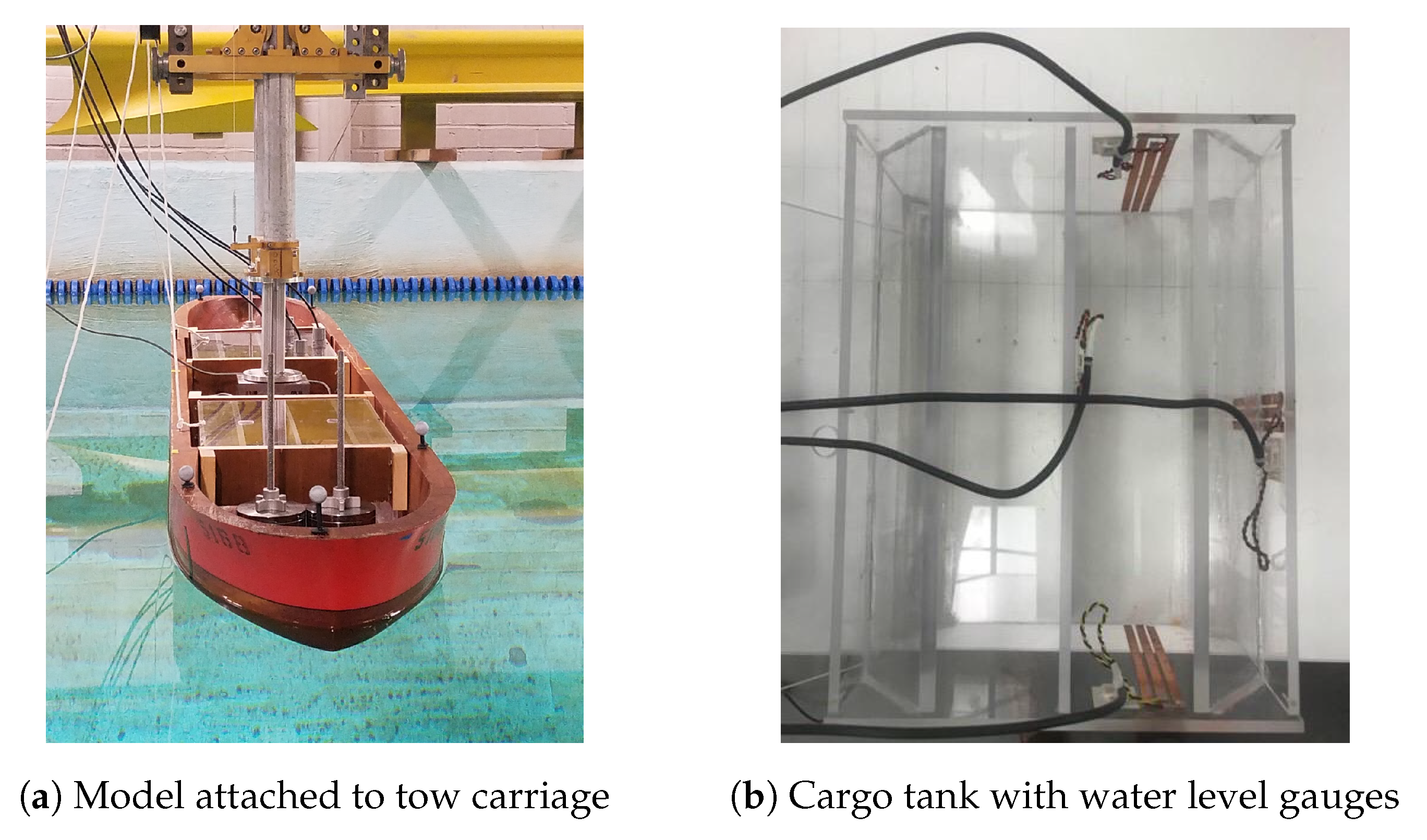
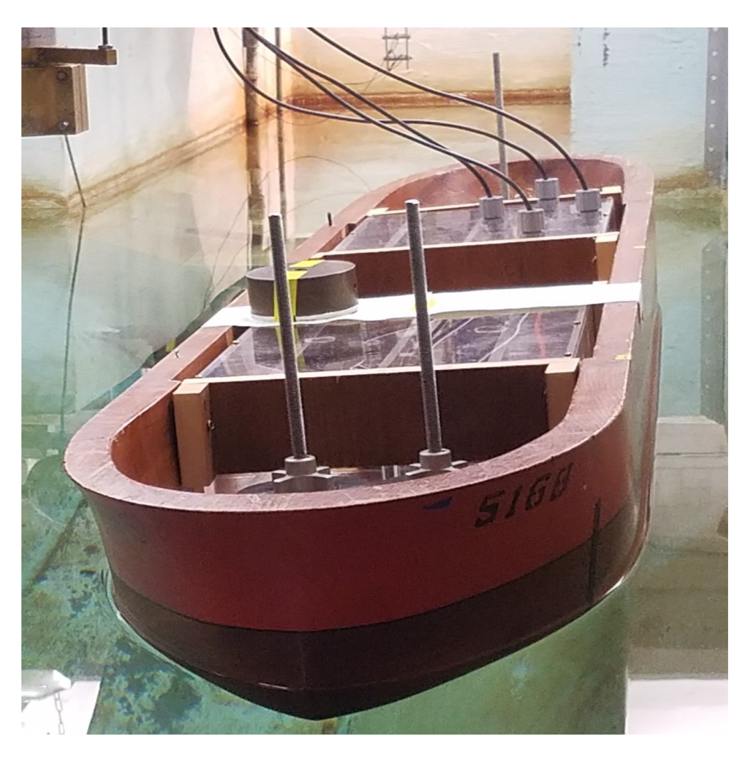
3.1. Model and Instrumentation

An existing tanker hull model made of wood is fitted with two two-row cargo tanks made of acrylic plates. The cargo tanks were placed in the model such that the sloshing occurs in the longitudinal axis of the tank during the roll motion. The model attached to the heave post and tow carriage is shown in Figure 8a. A roll pivot box is connected to the tow carriage to measure the roll amplitude and the walls of the port stern cargo tank is fitted with four water level gauges see Figure 8b to measure liquid water level in the tanks. All instrumentation used are calibrated prior to the test, see Appendix A. The main particulars of the model and cargo tanks are shown in Table 1. The draft of the vessel was measured at three locations; stern, amidships and the bow during the free floating inclining test and the roll decay tests and they are shown in Table A2.

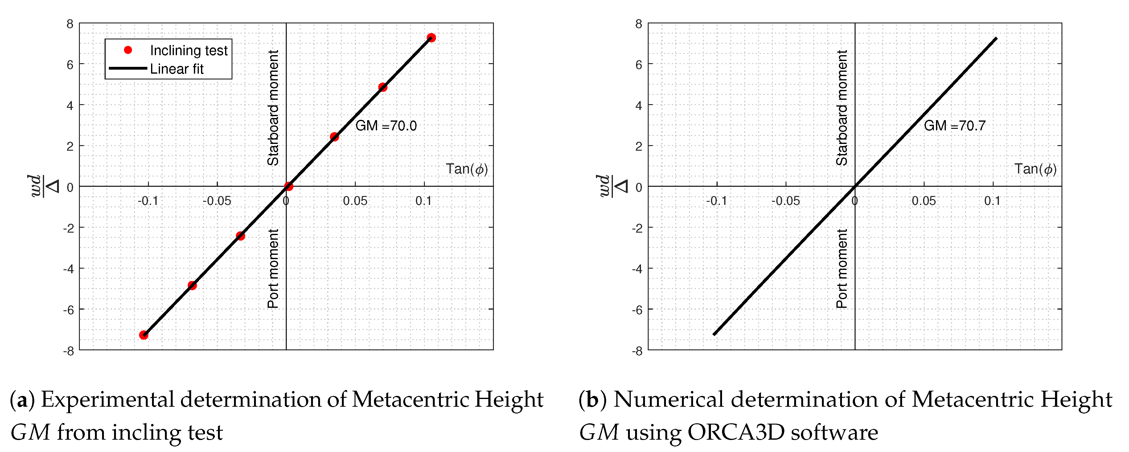
3.2. Inclination Test

To obtain the model’s vertical center of gravity K G , an inclining test was carried out in calm water by horizontally shifting an inclination mass of w i = 2.04 kg to the port and starboard sides with a horizontal shift d causing heeling angles [38]. The weight displacement were kept constant (inclination weight was taken from the loaded ballast) as shown in Figure 9, Figure A1 and Table A1. The Metacentric Height G M , was obtained using Equation (39) [38]. Table 2 shows the measured distances, the load moment per displacement, and the resulting roll angle. To get the vertical distance from the keel to the Metacenter K M , a hydrostatic analysis was conducted using ORCA3D [39] where the K M is evaluated at various vessel displacements. The vertical center of gravity K G 91.6 mm, was determined using Equation (40).
G M = w i d Δ tan φ
K G = K M G M
Figure 10a shows the inclining moment for the inclining tests with respect to the heeling angles φ , where a linear curve fitted to the dataset showed a slope of 70.0 mm representing the metacentric height G M as shown in Equation (39). Where Δ is the total displacement of the vessel in kg, see Table 1.
To validate the experimental inclining test, a reverse numerical inclining test was implemented in ORCA3D using K G from the experimental test and the same loading conditions. As shown in Figure 10b the numerical metacentric height for this loading case is 70.7 mm, confirming the experimental results.

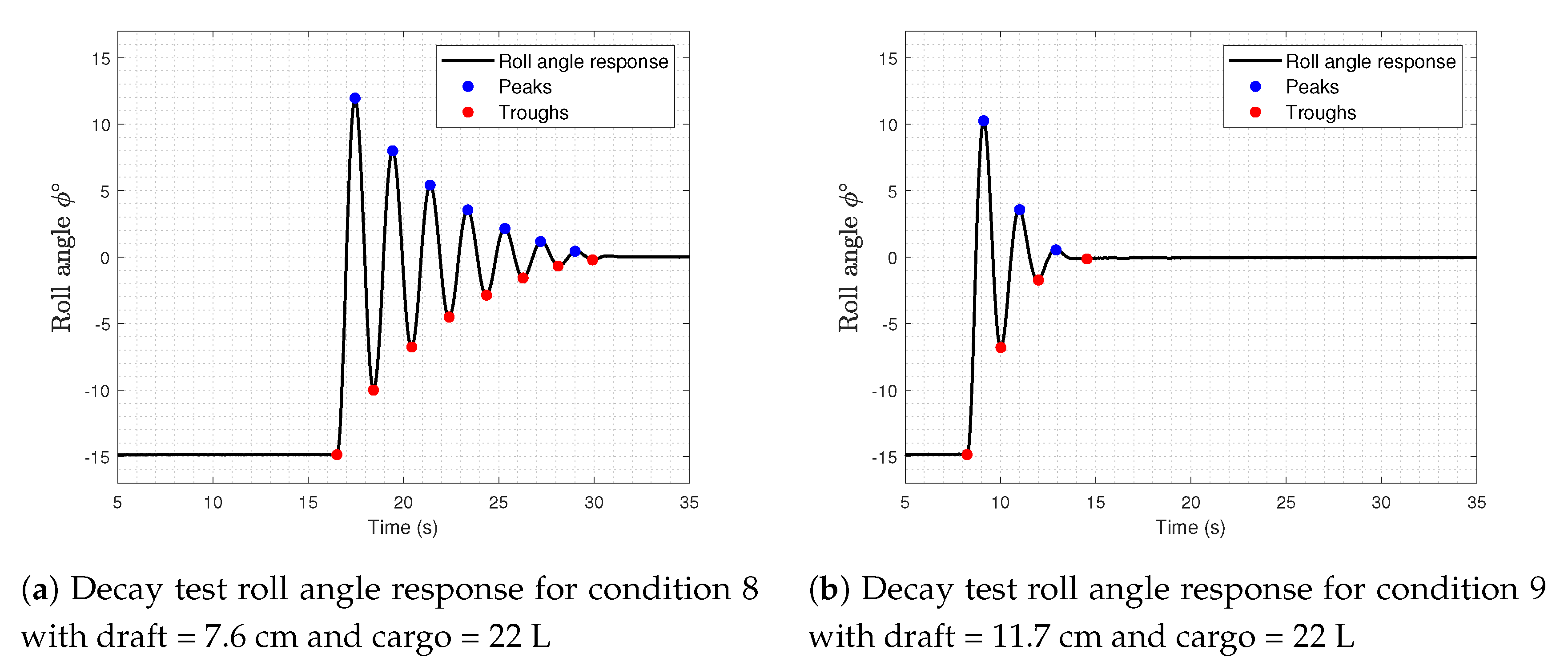
3.3. Roll Decay Test

The vessel roll decay experiment followed the guidelines and procedures by the International Marine Organisation (IMO) [40] and the International Towing Tank Conference (ITTC) [7] which advised that for highly damped vessels with low oscillation number, several roll tests (at least four) should be implemented with different initial roll angles, so the estimated damping coefficient would be continuous through the whole range of roll angle amplitudes. During the test, both two-row cargo tanks (4 compartments in total), were filled with water as shown in Table 3. The initial angle of the test was imposed by a system of pulley and strings as shown in Figure 8a and Figure A1. The volume displacement was kept constant (constant draft) for loading conditions 1–8 and the draft was increased for loading condition 9. The initial disturbance was between 7.3 and 17.7 , ITTC [7] recommends a disturbance larger than 25 , however it was not possible to achieve with the current experimental set up.
Roll amplitude was recorded by a rotational potentiometer installed inside the roll pivot box as shown in Figure A1. The model was allowed to roll freely after the release of the pulley-string system for all conditions, while sway, surge, yaw, pitch and heave were restricted.
To ensure no initial angular velocity nor unintended sloshing effect of the loaded water were induced, each test were performed for at least 3 minutes after the initial angle was set. Data collection was started before the release of pulley-string system to show the setup was at steady state prior to the test, in accordance with IMO and ITTC procedures [7,40].
To evaluate the repeatably of the the roll decay tests, some loading conditions were repeated with the same initial roll angle. The number of peaks and troughs before steady state for each repeated pairs are the same, however a deviation in the natural decay period is observed. Table 4 shows the percentage difference between each two measured natural periods, no dramatic deviation except for condition 8 where the cargo volume is at its maximum and the liquid sloshing on tanks wall is random in nature.

4. Results and Discussion

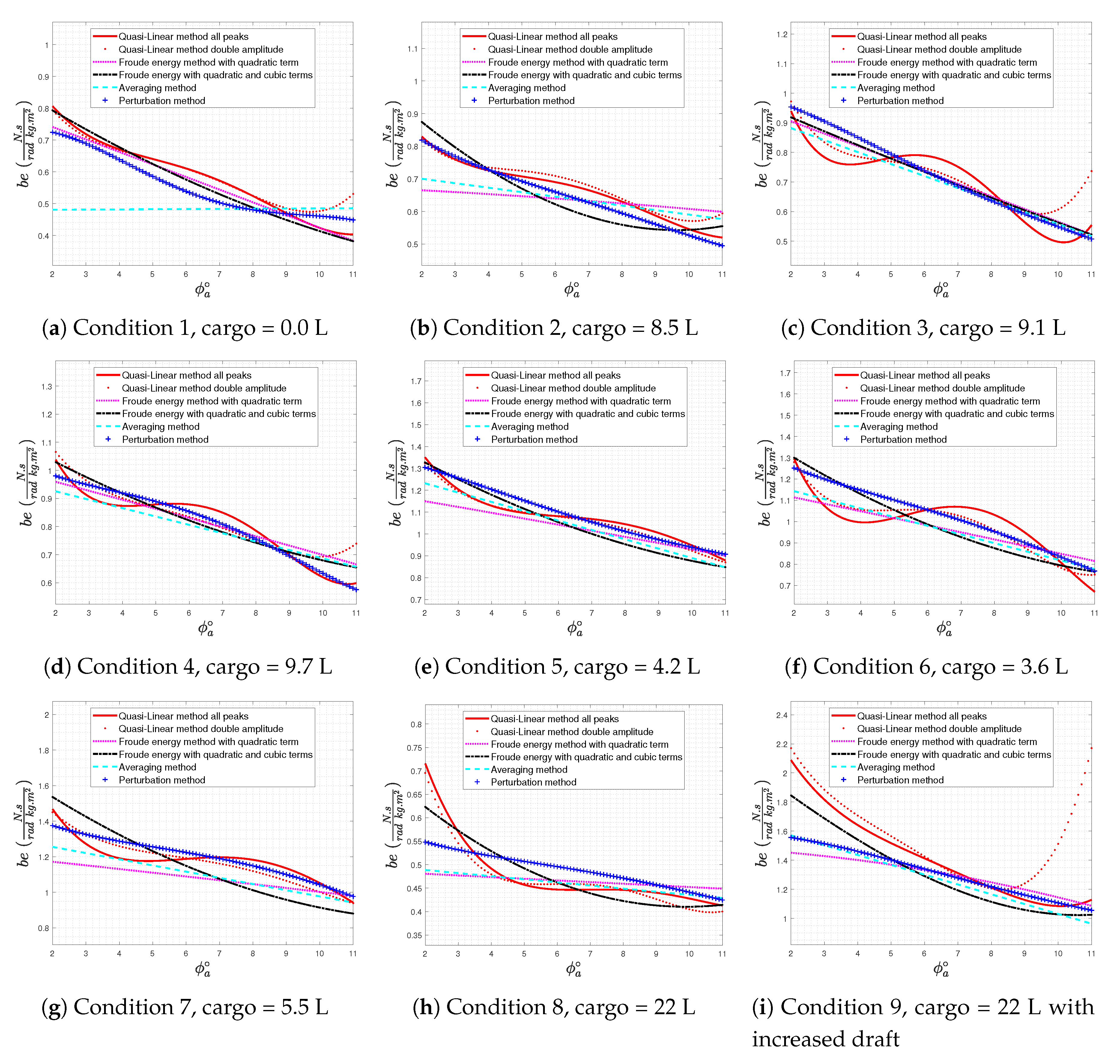
4.1. Effect of Analyzing Method

The equivalent linear damping coefficient per total mass moment of inertia ( b e ) is studied using the roll decay analysis methods presented in Section 2 for the 9 filling conditions described in Table 3 and Table A2. For most conditions and analysis methods, the equivalent linear damping coefficient is observed to have the same trend; it is inversely proportional to the roll angle amplitude as shown in Figure 11. As expected using the Averaging method, quadratic Froude energy method and Perturbation methods yields almost a linear relation between the equivalent linear damping coefficient and roll angle amplitude. However, for the Quasi-linear and cubic Froude energy methods where the cubic damping term is included, a nonlinear relation is observed, that implies that the cubic damping term can not be ignored for the tested vessel type.
A high deviation of the equivalent linear damping coefficient is observed when comparing the Averaging method and Froude energy method with quadratic and cubic terms at small roll angle amplitudes, across all loading conditions, see Figure 11. The Averaging method assumes that the motion is sinusoidal through the whole cycle, therefore it does not produce accurate results at lower angles where damping is high. The Froude energy method on the other hand assumes the motion is sinusoidal for only the cycle quarter and therefore produces more reliable results at low rolling angles [29]. At higher roll angle amplitudes, where the damping decreases, the Averaging method converges with the results from the other methods, this is expected and consistent across all loading conditions, since the Averaging method is recommended for lightly damped systems.

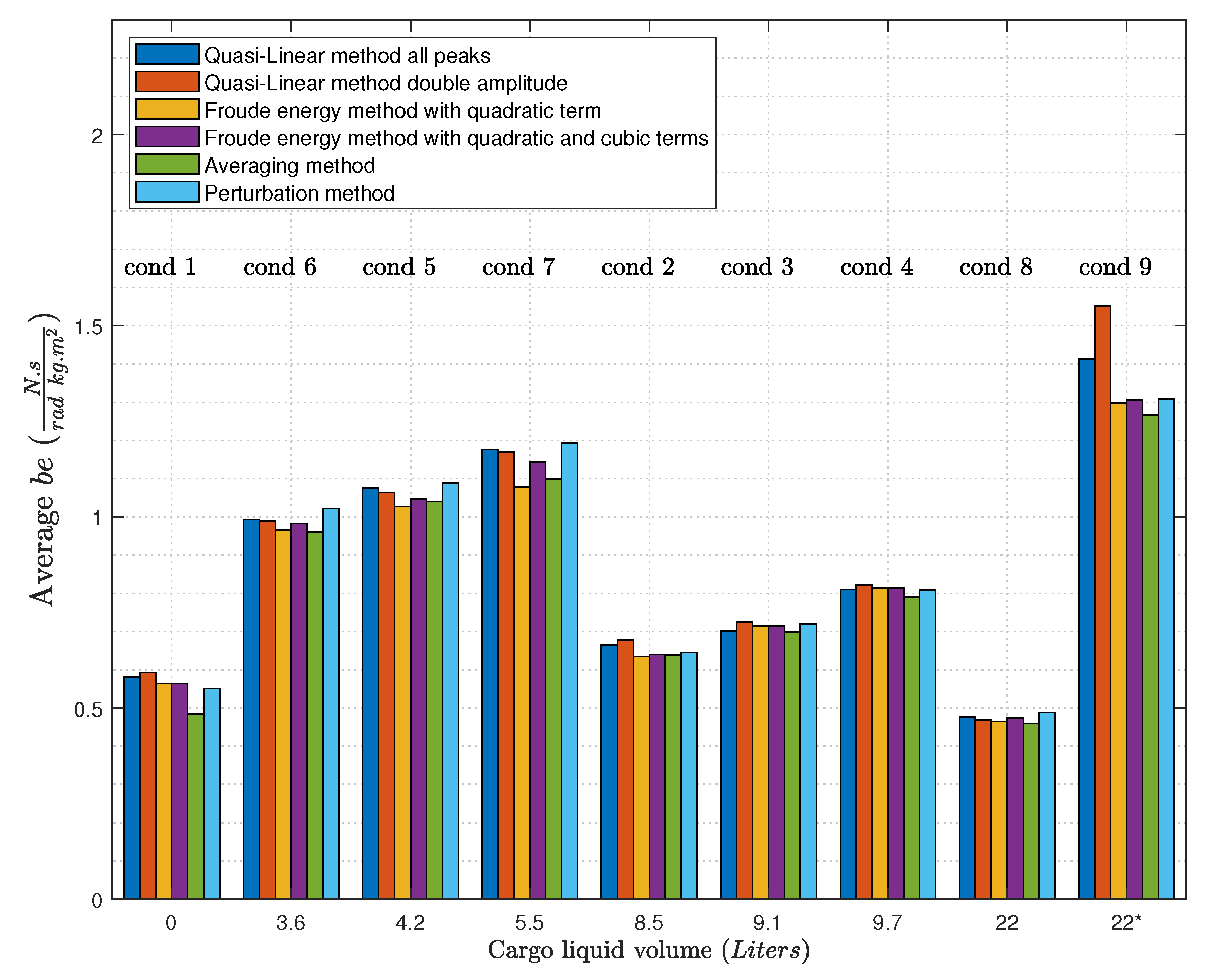
4.2. Effect of Liquid Cargo

Looking at results of the Quasi-linear method using all peaks and double amplitudes, a relation between the total cargo volume and the slope of the equivalent linear damping coefficient is observed at higher roll angle amplitudes. For low loading conditions [5, 6 and 7] (Figure 11e–g) the the equivalent linear damping coefficient has a negative slope at higher roll amplitude angles. On the other hand for the high loading conditions [2, 3, 4, 8 and 9] (Figure 11b–d,h,i) the damping coefficient show an inflection point nearly at the roll angle amplitude 10 followed by an increase. It should be noted that the change in dampening at higher filling levels [2, 3, 4, 8], is solely due to the increase in liquid cargo and thus liquid cargo motion, since the volume displacement is only changed in condition 9.
To evaluate the effect of the amount of liquid cargo on the vessel damping, a comparison is done between the mean linear equivalent damping coefficient for the whole range of rolling amplitudes and the volume of liquid cargo loading for the 9 loading conditions, see Figure 12. The results show that the vessel is highly dampened for cases of low filling volumes (conditions [6, 5 and 7]) where the liquid cargo sloshing forces’ effect on the tank walls does not affect the vessel motion. At condition 9, maximum condition with 22 L, and with increased draft, the vessel is observed to be very stable with the highest average equivalent damping coefficient due to the additional damping resistance applied by the increased draft. On the other hand and for high filling conditions [2, 3, 4 and 8], the cargo sloshing forces on tanks’ walls affected the dynamic behaviour of vessel rolling, where the equivalent linear damping coefficient decreased to about 50 percent compared to the very low filling conditions.

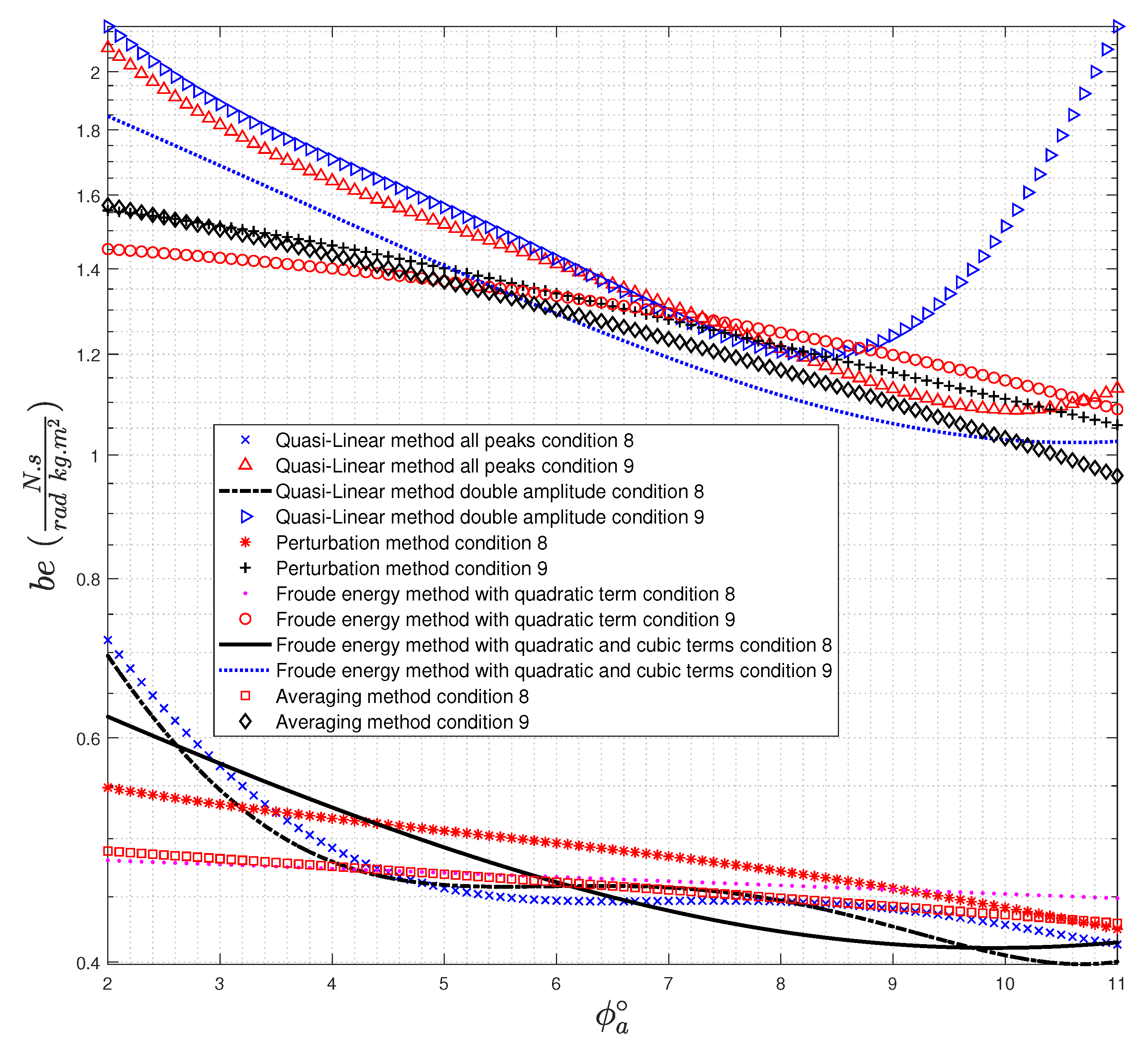
4.3. Effect of Volume Displacement

Increasing the draft from 7.8 cm (condition 8) to 11.7 cm (condition 9), while keeping the liquid cargo volume constant, a dramatic increase in the damping is seen (Figure 13a,b). Figure 13a,b show the decay roll angle response for the two conditions with initial heel angle ϕ 0 = 15 where condition 8 require twice as many oscillations compared with condition 9 to reach steady state. A comparison of the equivalent linear damping coefficient between conditions 8 and 9, is shown in Figure 14 where a dramatic increase of the damping is observed when the draft increased. Analyzing condition 8 using methods that considers both quadratic and cubic terms such as (Quasi-linear and Froude energy method with quadratic and cubic terms), it becomes clear that the damping coefficient has nonlinear behaviour as it slightly decreases with increasing roll amplitude, and beyond roll angle ϕ a = 5 the damping is almost constant. However, using methods that only considers the quadratic damping terms such as (Averaging, Perturbation and Froude energy with quadratic term) the damping coefficient is observed to be almost constant for the whole range of roll angle amplitudes as shown in Figure 14.

5. Conclusions

In this paper an experimental study was conducted to evaluate the equivalent linear damping coefficient of an FPSO vessel with liquid cargo in two two-row tanks at nine different filling levels. The equivalent linear damping was obtained using four different methods. To evaluate the effect of liquid cargo, the draft is kept constant for all but one loading condition. The model is highly damped, therefore multiple roll decay tests at different initial disturbance angle were needed to get a sufficient number of oscillations to obtain the equivalent linear damping.
The effect of liquid cargo volume in the two-row tanks on the vessel roll damping was investigated at constant draft. The results showed that the vessel damping is inversely proportional to the loaded cargo volume, an increase in the liquid cargo results in more liquid sloshing on the tanks walls which produces additional forcing moments, thus increasing the rolling motion and decreasing the vessel damping.
For most of the tested cases, the linear equivalent damping coefficient is observed to be inversely proportional to the roll angle amplitude. As expected, the relationship between the roll angle and equivalent linear damping coefficient depends on the analyzing method; methods that only accounts for the linear and quadratic damping terms such as quadratic Froude energy method, Averaging method and Perturbation method, show a linear relationship. However a nonlinear relation is seen when using methods that accounts for the cubic damping term such as, Quasi-linear method and quadratic-cubic Froude energy method. This implies that the cubic damping term is necessary for this vessel type.
There are no dramatic differences between different roll decay test analysis methods for estimation the equivalent linear damping coefficient except the Averaging method that underestimates the coefficient for this highly dampened system.
The perturbation method is accurate in determining the linear and non-linear damping coefficients but it requires three unknown exponential curve fitting for the decay envelope. Hence, it is recommended to be used for roll decay tests that have large number of oscillations to ensure robust and stable curve fitting or the the curve fitting algorithm should be constrained for an expected range of the unknown values to be estimated.
Therefore, the Froude energy and the Quasi-linear methods are recommended, as they are able to compute the damping coefficient with no restrictions with regards to the system dampening (high or low), nor do they require a large number of peaks (minimum three). The Quasi-linear method has an advance over the Froude energy method; no curve fitting is required and the equivalent damping coefficient is computed directly with minimum.

Author Contributions

Conceptualization, J.-F.I. and M.F.; methodology, J.-F.I., O.S., M.F. and R.F.; software, O.S., M.F. and R.F.; validation, O.S. and M.F.; formal analysis, O.S.; investigation, J.-F.I., O.S., M.F. and R.F.; resources, M.F.; data curation, J.-F.I., O.S., M.F. and R.F.; writing—original draft preparation, J.-F.I., O.S., M.F. and R.F.; writing—review and editing, J.-F.I., O.S., M.F. and R.F.; visualization, J.-F.I., O.S., M.F. and R.F.; supervision, M.F.; project administration, M.F.; funding acquisition, J.-F.I. All authors have read and agreed to the published version of the manuscript.

Funding

This research was funded by Petroleum Technology Development Fund (PTDF) Nigeria.

Acknowledgments

Appreciation goes to the Petroleum Technology Development Fund (PTDF) Nigeria, Davidson Laboratory research group and members of Furth Lab, Stevens Institute of Technology.

Conflicts of Interest

The authors declare no conflict of interest.

Appendix A. Test Equipment
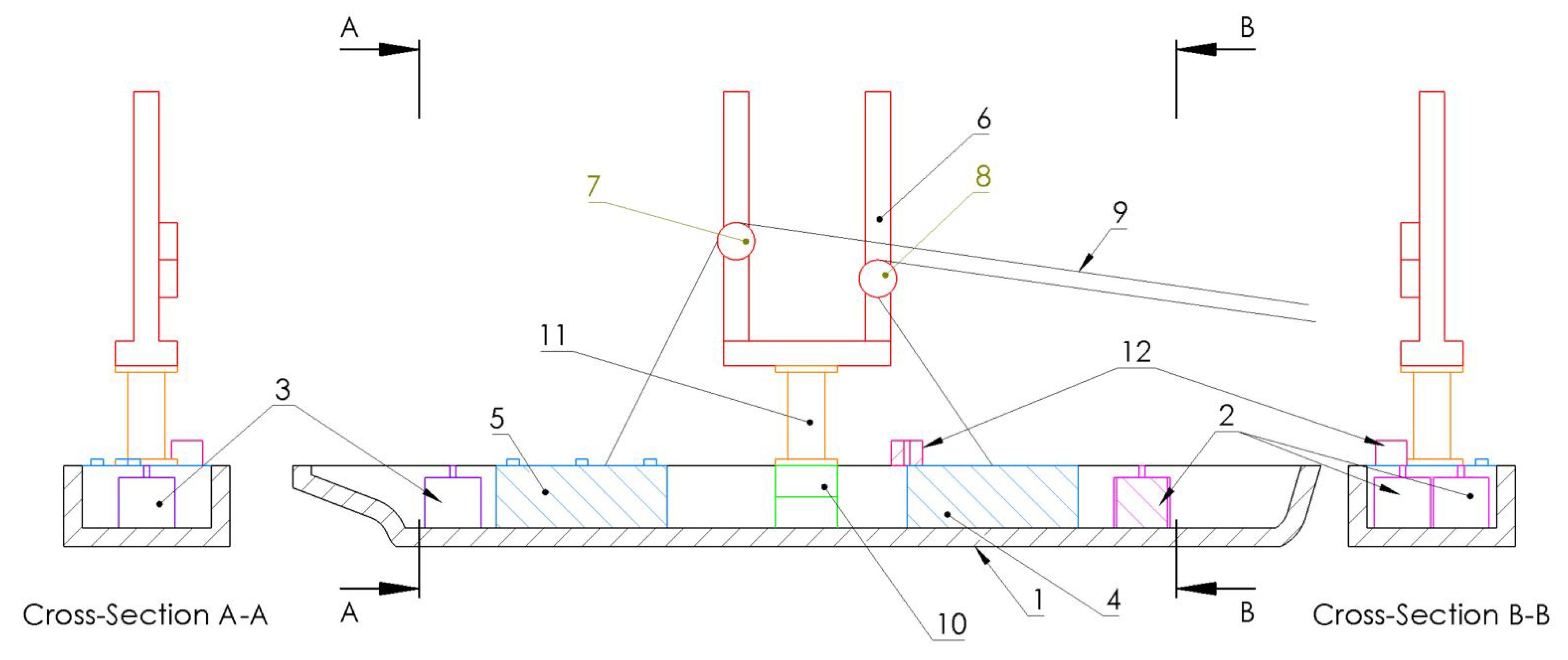
The locations of the ballast and measuring equipment used for the roll decay test are shown in Figure A1 and Table A1. All locations are measured from the aft longitudinally and from the keel for vertical distances. The model was fixed in sway, surge, yaw, pitch and heave, while free to roll. For condition 1 to 8, the model was locked in heave, fixing the draft at the unloaded ballasted condition. For condition 9, sinkage was allowed by temporarily releasing the heave restrain, after the model reached the draft required to support the load heave was again clamped.
The model was free floating (not attached to the have post) for the inclination test, at the ballasted loading condition. Pivot box and drag balance (10), attachment bar (11) were not loaded in inclination test. The ballast weight distribution and incline weight (12) during the test is shown in Figure A1 and Table A1.
Table A1. Devices and Locations.
Unit Name and Figure NumberLCG [mm] from AftVCG [mm] from KeelMass [Kg]
FPSO Hull (1) with Ballast (2 and 3)1136.091.624.10
and Empty Cargo Tanks (4 and 5)
Forward Ballasts (2)
(Roll Decay Test)
Port Ballast (TCG = 44.45 mm)1771.65117.814.72
Starboard Ballast (TCG = −44.45 mm)1771.65117.814.72
(Inclination Test)
Port Ballast (TCG = 44.45 mm)1771.65110.304.15
Starboard Ballast (TCG = −44.45 mm)1771.65110.304.15
Aft Ballast (3)
(Roll Decay Test)400.05129.815.67
(Inclination Test)400.05121.804.77
Forward Cargo Tank (4)770.64VariesVaries
Aft Cargo Tank (5) with Water Level Gauges1529.08VariesVaries
Heave Post (6) with Pulleys and clamps (7 and 8)412.50685.803.20
Pivot Box and Drag Balance (10)412.50190.553.88
Attachment Bar (11)1677.92304.80.71
Incline Weight (12)1328.42280.802.04
Strings used to induce roll (9)
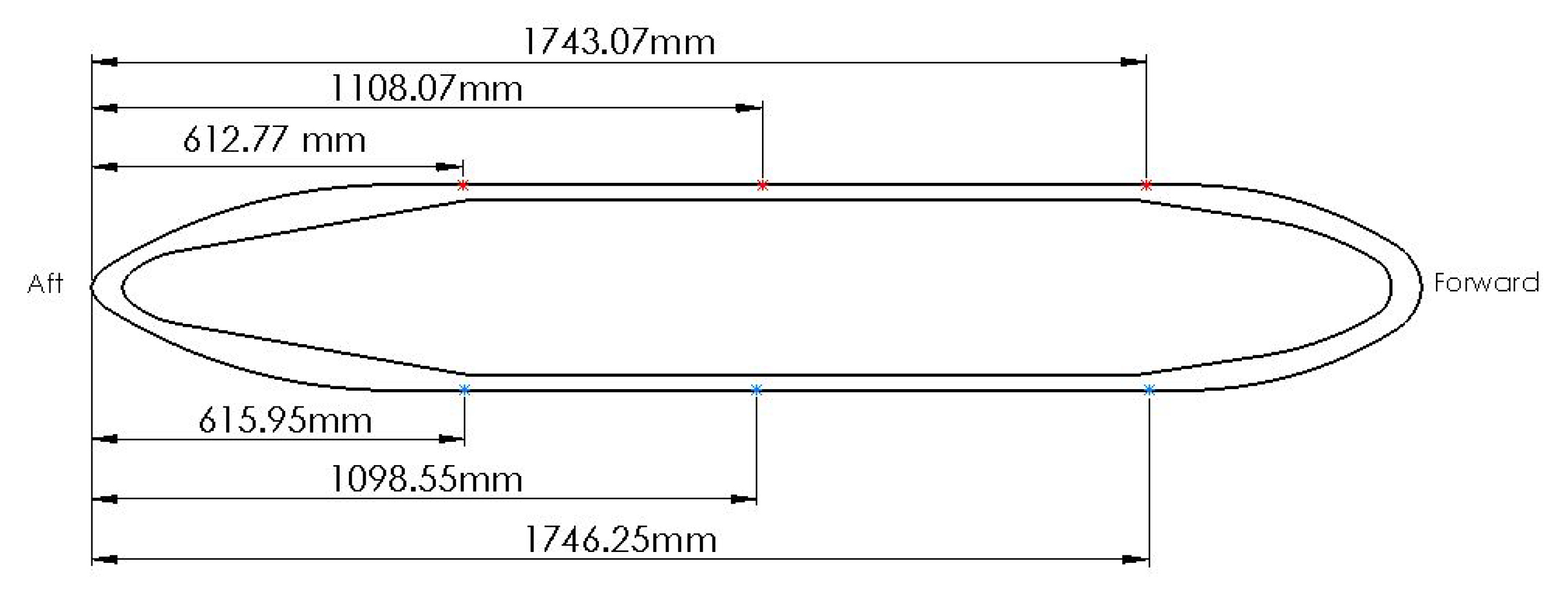
Figure A1. Position of sensors and weights in the model.
Jmse 08 00582 g0a1
Table A2. Draft and draft measuring locations from Aft.
Incline Test
(Port)
Location (mm)612.771108.071743.07
Draft (mm)666666
Roll Decay Test
(Starboard)
Location (mm)615.951098.551746.25
Draft (mm)Condition 1–8707881
Condition 9105117125
Figure A2. Measuring Locations.
Jmse 08 00582 g0a2
Figure A3. Schematic of Cargo Tank.
Jmse 08 00582 g0a3

Appendix A.1. Ballast Weight and Weight Posts

The ballast weight were secured on three weight post, two in the forward and one in the aft as shown in Figure A1. The weight posts were fixed on the bottom of the model to minimize the motion induced by the ballast.

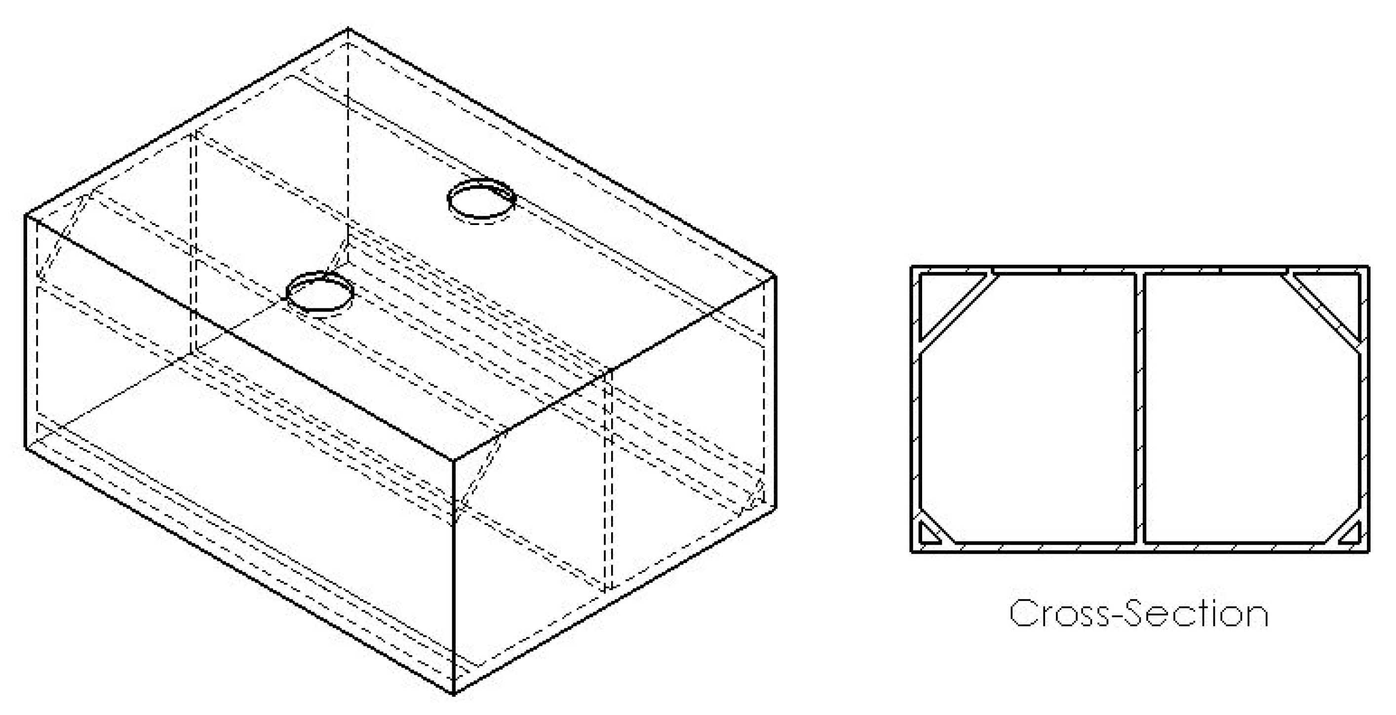
Appendix A.2. Cargo Tank

Two two-row tanks were installed in the forward and aft of the model as shown in Figure A1. The tanks consisted of two separated compartments, shown in Figure A3, one on the port side and one on the starboard side. The tank was machined with angled edges as shown in Figure A3 to reduce corner sloshing effect. Four water level gauges were installed at the center line of four walls in the port compartment of the aft cargo tank.

Appendix A.3. Towing Carriage and Heaving Post

Towing carriage was served as a testing platform in the roll decay test. Sensors, camera, heave post, pivot box and the model itself were attached to the carriage. The primary use of the carriage is to record the roll angle and to fix the movement of the model in surge, sway, yaw and heave. The heave post and the attachment bar are the component connecting the model to the towing carriage, see Figure A1. A pulley system was setup on the model for roll decay test as shown in Figure A1. Two pulleys were fixed on the heave post and two strings were secured on the starboard side of the model. To ensure a quick release during the test, the string selected has low flexibility and a weight realise system was implemented to avoid slack.

Appendix A.4. Pivot Box

The Pivot Box is attached to the base plate of the model and orientated so that only roll was allowed. The included rotational potentiometer is the primary method to measure roll in the roll decay test. The potentiometer is calibrated to statically to within an accuracy of ±0.18 degrees.

References

  1. Balthazar, J.M.; Gonçalves, P.B.; Lenci, S.; Mikhlin, Y.V. Models, Methods, and Applications of Dynamics and Control in Engineering Sciences: State of the Art. Math. Probl. Eng. 2010, 2010. [Google Scholar] [CrossRef] [Green Version]
  2. Guze, S.; Wawrzynski, W.; Wilczynski, P. Determination of Parameters Describing the Risk Areas of Ships Chaotic Rolling on the Example of LNG Carrier and OSV Vessel. J. Mar. Sci. Eng. 2020, 8, 91. [Google Scholar] [CrossRef] [Green Version]
  3. Kim, Y.; Park, M.J. Identification of the nonlinear roll damping and restoring moment of a FPSO using Hilbert transform. Ocean Eng. 2015, 109, 381–388. [Google Scholar] [CrossRef]
  4. Arai, M.; Cheng, L.; Inoue, Y.; Sasaki, H.; Yamagishi, N. Numerical analysis of liquid sloshing in tanks of FPSO. In Proceedings of the Second International Offshore and Polar Engineering Conference, San Francisco, CA, USA, 14–19 June 1992. [Google Scholar]
  5. Zhao, W.; Efthymiou, M.; McPhail, F.; Wille, S. Nonlinear roll damping of a barge with and without liquid cargo in spherical tanks. J. Ocean Eng. Sci. 2016, 1, 84–91. [Google Scholar] [CrossRef] [Green Version]
  6. Chakrabarti, S. Empirical calculation of roll damping for ships and barges. Ocean Eng. 2001, 28, 915–932. [Google Scholar] [CrossRef]
  7. ITTC. Numerical estimation of roll damping. In Proceedings of the 26th International Towing Tanks Conference, Rio de Janeiro, Brazil, 28 August–3 September 2011. Number 7.5-02-07-04.5. [Google Scholar]
  8. Salvesen, N.; Tuck, E.; Faltinsen, O. Ship Motions and Sea Loads; The Society of Naval Architects and Marine Engineers: New York, NY, USA, 1970. [Google Scholar]
  9. Prpić-Oršić, J.; Čorić, V. Seakeeping; University of Rijeka: Rijeka, Croatia, 2006. [Google Scholar]
  10. Guo, Z.; Ma, Q.; Yu, S.; Qin, H. A body-nonlinear Green’s function method with viscous dissipation effects for large-amplitude roll of floating bodies. Appl. Sci. 2018, 8, 517. [Google Scholar] [CrossRef] [Green Version]
  11. Froude, W.; Abell, S.W.; Gawn, R.; Duckworth, A. The Papers of William Froude, 1810–1879: With a Memoir by Sir Westcott Abell and an Evaluation of William Froude’s Work by RWL Gawn: Collected Into One Volume; Institution of Naval Architects: London, UK, 1955. [Google Scholar]
  12. Ikeda, Y.; Himeno, Y.; Norio, T. A prediction method for ship roll damping. In Report No. 00405 of the Department of Naval Architecture; University of Osaka Prefecture: Osaka, Japan, 1978. [Google Scholar]
  13. Kianejad, S.; Lee, J.; Liu, Y.; Enshaei, H. Numerical assessment of roll motion characteristics and damping coefficient of a ship. J. Mar. Sci. Eng. 2018, 6, 101. [Google Scholar] [CrossRef] [Green Version]
  14. Remola, A.O. On Ship Roll Damping: Analysis and Contributions on Experimental Techniques. Ph.D. Thesis, Universidad Politécnica de Madrid, Madrid, Spain, 2018. [Google Scholar]
  15. Handschel, S.; Feder, D.F.; Abdel-Maksoud, M. Estimation of ship roll damping-A comparison of the decay and the harmonic excited roll motion technique for a post panamax container ship. In Proceedings of the 12th International Conference on the Stability of Ships and Ocean Vehicles, Glasgow, UK, 14–19 June 2015; pp. 475–488. [Google Scholar]
  16. Bačkalov, I.; Bulian, G.; Cichowicz, J.; Eliopoulou, E.; Konovessis, D.; Leguen, J.F.; Rosén, A.; Themelis, N. Ship stability, dynamics and safety: Status and perspectives from a review of recent STAB conferences and ISSW events. Ocean Eng. 2016, 116, 312–349. [Google Scholar] [CrossRef]
  17. Kinnas, S.A.; Yi-Hsiang, Y.; Vinayan, V. Prediction of flows around FPSO hull sections in roll using an unsteady Navier-Stokes solver. In Proceedings of the Sixteenth International Offshore and Polar Engineering Conference, San Francisco, CA, USA, 28 May–2 June 2006. [Google Scholar]
  18. Thiagarajan, K.P.; Braddock, E.C. Influence of bilge keel width on the roll damping of FPSO. J. Offshore Mech. Arct. Eng. 2010, 132, 011303-1–011303-7. [Google Scholar] [CrossRef]
  19. Blume, P. Experimentell bestimmung von koeffizienten der wirksamen rolldämpfung und ihre anwedung zur abschätzung extremer rollwinkel. In Institut für Schiffbau, Universität Hamburg, Bericht Nr. 1511, Zeitschrifft “Schiffstechnik’, Band 26, 1979; Universität Hamburg: Hamburg, Germany, 1979. [Google Scholar]
  20. Handschel, S.; Abdel-Maksoud, M. Improvement of the harmonic excited roll motion technique for estimating roll damping. Ship Technol. Res. 2014, 61, 116–130. [Google Scholar] [CrossRef]
  21. Wassermann, S.; Feder, D.F.; Abdel-Maksoud, M. Estimation of ship roll damping—A comparison of the decay and the harmonic excited roll motion technique for a post panamax container ship. Ocean Eng. 2016, 120, 371–382. [Google Scholar] [CrossRef]
  22. Avalos, G.O.; Wanderley, J.B. A Two-Dimensional Numerical Simulation of Roll Damping Decay of a FPSO Using the Upwind TVD Scheme of Roe-Sweby. In International Conference on Offshore Mechanics and Arctic Engineering; American Society of Mechanical Engineers: New York, NY, USA, 2012; Volume 44915, pp. 395–402. [Google Scholar]
  23. Avalos, G.O.; Wanderley, J.B.; Fernandes, A.C.; Oliveira, A.C. Roll damping decay of a FPSO with bilge keel. Ocean Eng. 2014, 87, 111–120. [Google Scholar] [CrossRef]
  24. Zhou, Y.H.; Ma, N.; Shi, X.; Zhang, C. Direct calculation method of roll damping based on three-dimensional CFD approach. J. Hydrodyn. 2015, 27, 176–186. [Google Scholar] [CrossRef]
  25. Gu, Y.; Boulougouris, E.; Day, A. A Study on the Effects of Bilge Keels on Roll Damping Coefficient. In Proceedings of the 12th International Conference on the Stability of Ships and Ocean Vehicles, Glasgow, UK, 14–19 June 2015. [Google Scholar]
  26. Rodríguez, C.A.; Esperança, P.T.; Oliveira, M.C. Estimation of Roll Damping Coefficients Based on Model Tests Responses of a FPSO in Waves. In International Conference on Offshore Mechanics and Arctic Engineering; American Society of Mechanical Engineers: New York, NY, USA, 2019; Volume 58851, p. V07BT06A021. [Google Scholar]
  27. Zeraatgar, H.; Asghari, M.; Bakhtiari-Nejad, F. A study of the roll motion by means of a free decay test. J. Offshore Mech. Arct. Eng. 2010, 132, 031303. [Google Scholar] [CrossRef]
  28. Oliva-Remola, A.; Bulian, G.; Pérez-Rojas, L. Estimation of damping through internally excited roll tests. Ocean Eng. 2018, 160, 490–506. [Google Scholar] [CrossRef]
  29. Spouge, J. Non-linear analysis of large-amplitude rolling experiments. Int. Shipbuild. Prog. 1988, 35, 271–324. [Google Scholar]
  30. Bulian, G. Estimation of nonlinear roll decay parameters using an analytical approximate solution of the decay time history. Int. Shipbuild. Prog. 2004, 51, 5–32. [Google Scholar]
  31. ESilva, S.R.; Soares, C.G. Prediction of parametric rolling in waves with a time domain non-linear strip theory model. Ocean Eng. 2013, 72, 453–469. [Google Scholar]
  32. Uzunoglu, E.; Soares, C.G. Automated processing of free roll decay experimental data. Ocean Eng. 2015, 102, 17–26. [Google Scholar] [CrossRef]
  33. Sun, J.; Shao, M. Estimation of Nonlinear Roll Damping by Analytical Approximation of Experimental Free-Decay Amplitudes. J. Ocean Univ. China 2019, 18, 812–822. [Google Scholar] [CrossRef]
  34. Roberts, J.B. Estimation of Non-Linear Ship Roll Damping from Free-Decay Data; Technical Report; Journal of Ship Research, Vol. 29, No. 2; The Society of Naval Architects and Marine Engineers; University of Sussex: Brighton, UK, 1985; pp. 127–138. [Google Scholar]
  35. Flower, J.; Sabti Aljaff, W. Kryloff-Bogoliuboff’s solution to decaying nonlinear oscillations in marine systems. Int. Shipbuild. Prog. 1980, 27, 225–230. [Google Scholar] [CrossRef]
  36. Himeno, Y. Prediction of Ship Roll Damping—A State of the Art; Technical Report; University of Michigan: Ann Arbor, MI, USA, 1981. [Google Scholar]
  37. Dalzell, J. A Note on the Form of Ship Roll Damping; Technical Report; Stevens Inst of Tech Hoboken N Davidson Lab.: Hoboken, NJ, USA, 1976. [Google Scholar]
  38. Zubaly, R.B. Applied Naval Architecture; Cornell Maritime Press, Schiffer Publishing, Ltd.: Atglen, PA, USA, 1996. [Google Scholar]
  39. Solutions, D.D. ORCA3D User Manual; DRS Technology: Largo, FL, USA, 2015. [Google Scholar]
  40. Iqbal, K.S.; Bulian, G.; Hasegawa, K.; Karim, M.; Mashud, A. Interim guidelines for alternative assessment of the weather criterion Interim guidelines for alternative assessment of the weather criterion, 2006. J. Mar. Sci. Technol. 2008, 13, 282–290. [Google Scholar] [CrossRef]
Figure 1. Roll angle decay response with peaks and double amplitudes annotations test case 8, see Section 3.3.
Jmse 08 00582 g001
Figure 2. Equivalent linear damping coefficient estimation using quasi-linear method Equation (12), test case 8 by combining results of 4 tests with different initial roll angles, see Section 3.3.
Jmse 08 00582 g002
Figure 3. Annotation of peak and trough amplitudes for half cycle, test case 8, see Section 3.3.
Jmse 08 00582 g003
Figure 4. Equivalent linear damping coefficient estimation using Froude energy method with linear and quadratic damping terms, test case 8 by combining results of 4 tests with different initial roll angles, see Section 3.3. (a) Estimation of extinction coefficients a and b using quadratic curve fitting, Equation (22); (b) Equivalent linear damping coefficient b e estimation based on the extinction coefficients a and b using Equation (23).
Jmse 08 00582 g004
Figure 5. Equivalent linear damping coefficient estimation using Froude energy method with linear, quadratic and cubic damping terms, test case 8 by combining results of 4 tests with different initial roll angles, see Section 3.3. (a) Estimation of extinction coefficients a, b and c using cubic curve fitting, Equation (22); (b) Equivalent linear damping coefficient b e estimation based on the extinction coefficients a, b and c using Equation (23).
Jmse 08 00582 g005
Figure 6. Equivalent linear damping coefficient estimation using Averaging method, test case 8 by combining results of 4 tests with different initial roll angles, see Section 3.3. (a) Estimation of A, B coefficients using quadratic curve fitting between d ϕ a d t and ϕ a Equation (27); (b) Equivalent linear damping coefficient b e estimation based on b 1 and b 2 using Equations (28).
Jmse 08 00582 g006
Figure 7. Equivalent linear damping coefficient estimation using the perturbation method, test case 8, see Section 3.3. (a) Roll angle decay test envelope nonlinear curve fitting with Equation (37); (b) Equivalent linear damping coefficient using the estimated coefficients b 1 and b 2 Equation (38).
Jmse 08 00582 g007
Figure 8. Model attached to heave post and cargo tank.
Jmse 08 00582 g008
Figure 9. Model during Incline Test.
Jmse 08 00582 g009
Figure 10. Determination of Metacentric Height G M from experimental inclining test data and numerical modelling using ORCA3D software.
Jmse 08 00582 g010
Figure 11. Equivalent linear damping coefficient determined using different analysis methods as a function of roll angle amplitude for different liquid loading conditions.
Jmse 08 00582 g011
Figure 12. Average equivalent damping coefficient b e and as a function of the liquid cargo volume for the different test conditions. Note that conditions 8 and 9 have the same cargo volume but different draft, see Table 3 and Table A2.
Jmse 08 00582 g012
Figure 13. Effect of vessel draft on the dynamic response of the FPSO model during roll decay test.
Jmse 08 00582 g013
Figure 14. The effect of the vessel draft on the equivalent linear damping coefficient b e using different decay analysis methods. Condition 8 has a shallow draft equivalent to an unloaded vessel, condition 9 has a draft equivalent to a fully loaded vessel. In both conditions all tanks have a 95 ± filling level.
Jmse 08 00582 g014
Table 1. FPSO and cargo tank characteristics.
ParameterValueUnit
Length overall LOA2.18m
Beam B0.341m
Depth D0.19m
Unballasted vessel weight24.96kg
Ballasted vessel weight40kg
Displacement (ballast condition) Δ m 0.029ton
Kyy1.09m
Kzz1.09m
Kxx0.12m
Cargo Tank Outer Dimensions
Length L T 0.49m
Width B T 0.26m
Width of one tank B T 1 0.13m
Depth D T 0.17m
Thickness t0.01m
Table 2. Inclination test.
SideLoad Horizontal Shift d (mm)Load Moment per Displacement wd Δ (mm)Roll Angle ϕ
−150−78−5.9
Port side−100−52−3.9
−50−26−1.9
000.1
50262.0
Starboard side100524.0
150786.0
Table 3. Water Tank Loading Conditions.
ForwardAft
ConditionPortStarboardPortStarboard
VolumePercentageVolumePercentageVolumePercentageVolumePercentage
(L)(%)(L)(%)(L)(%)(L)(%)
100000000
2003505.59500
3000.6103505.595
40.6105.5953500.610
5350000.6100.610
635000000.610
75.595000000
85.5955.5955.5955.595
9 *5.5955.5955.5955.595
* Sinkage was allowed for Condition 9 as shown in Table A2 and Figure A2.
Table 4. Natural decay period for conditions with the same initial roll angle.
ConditionInitial Roll Angle φ ± 0.1 Natural Period (s)Percentage Difference %
316.61.686.13
1.58
512.61.2610
1.14
713.61.306.35
1.22
816.61.6225.3
2.09

