Enhanced Control Scheme for a Three-Phase Grid-Connected PV Inverter under Unbalanced Fault Conditions

 ,
, 
Abstract
:1. Introduction
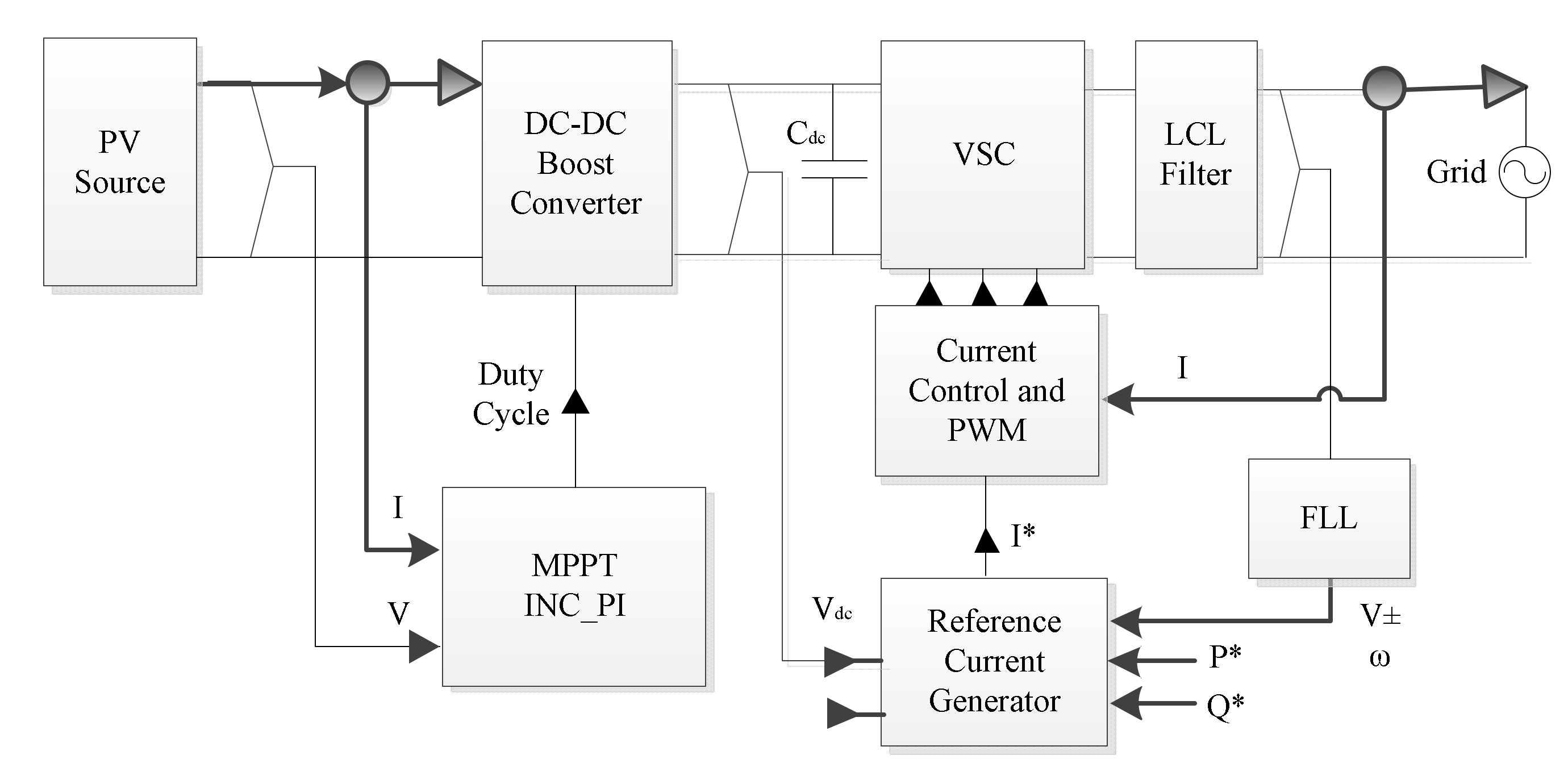
2. PV System Modeling
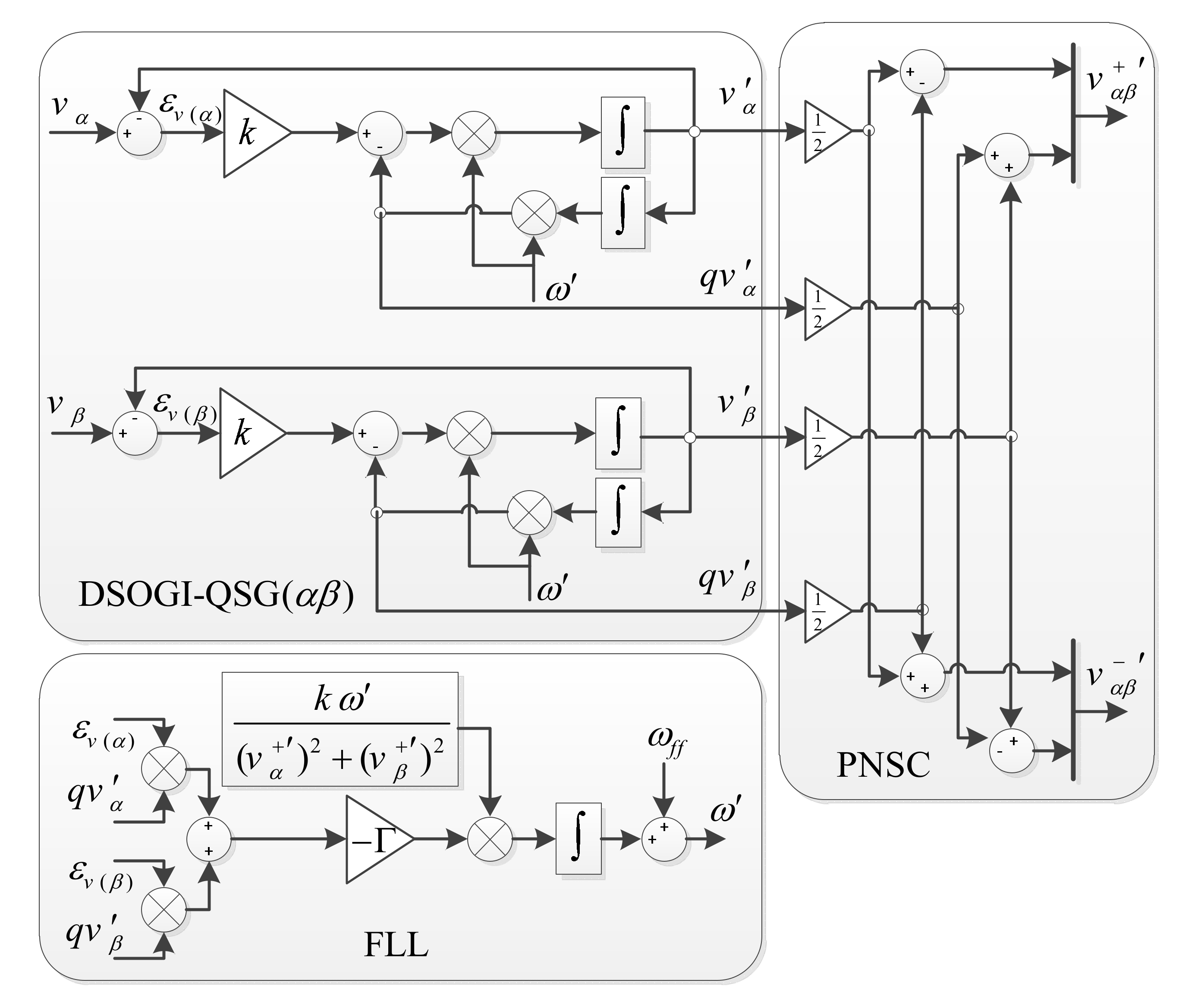
2.1. FLL Synchronization System
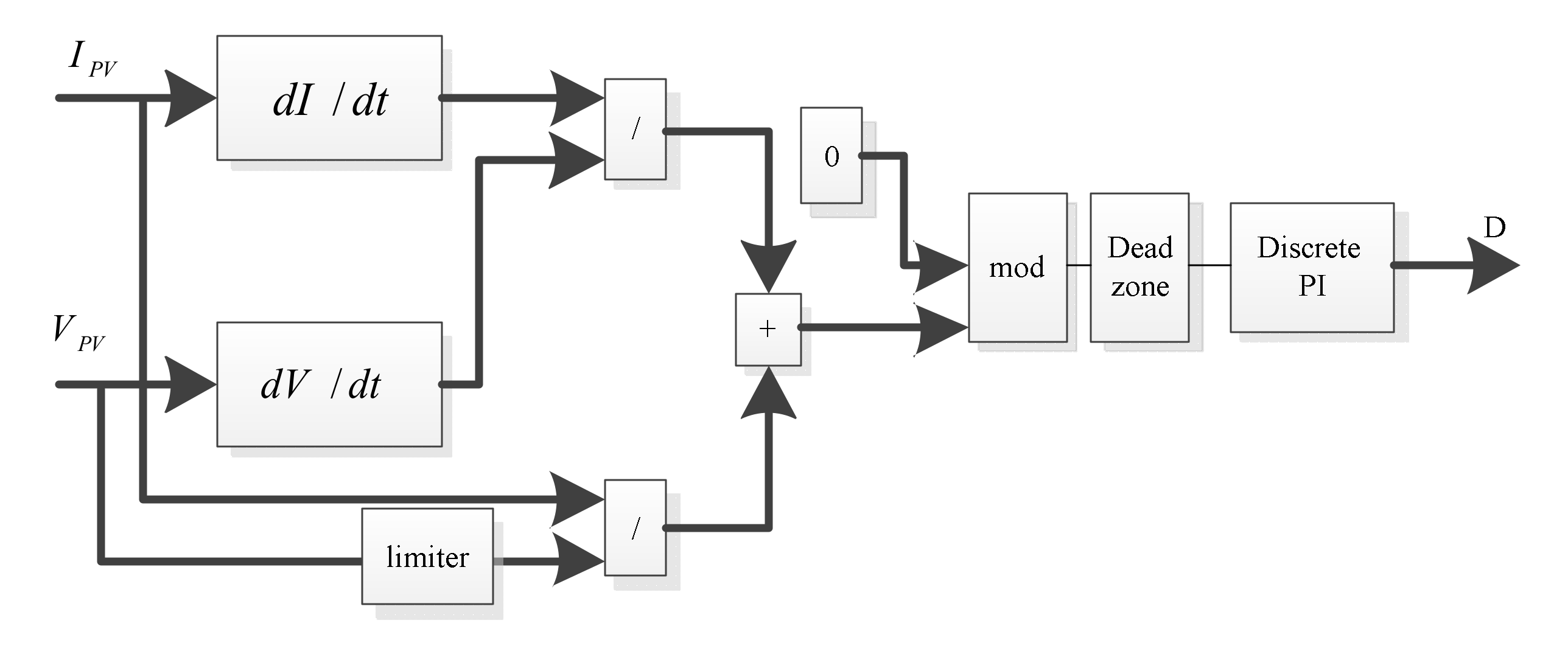
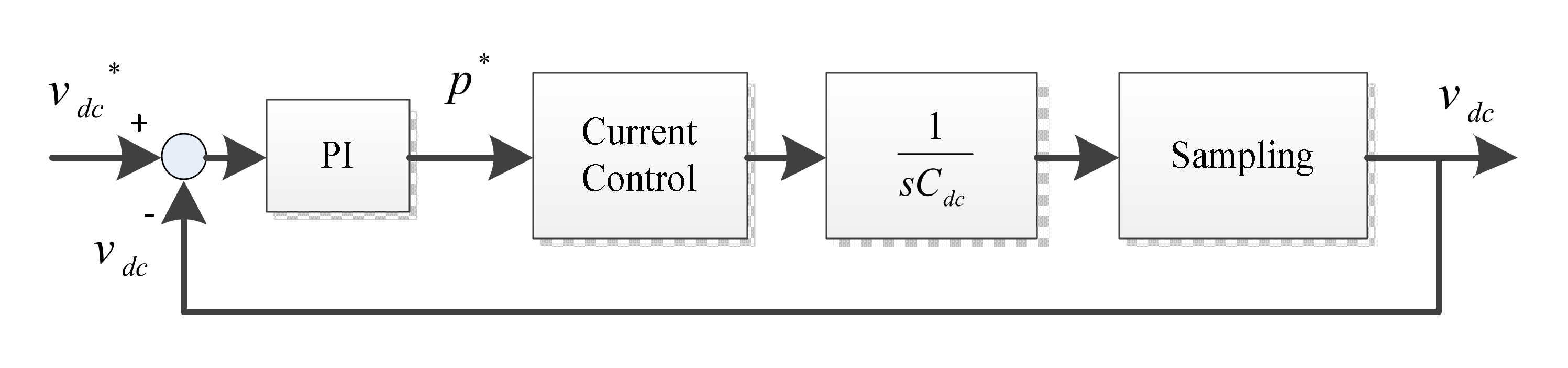
2.2. MPPT Method
2.3. Current Controller
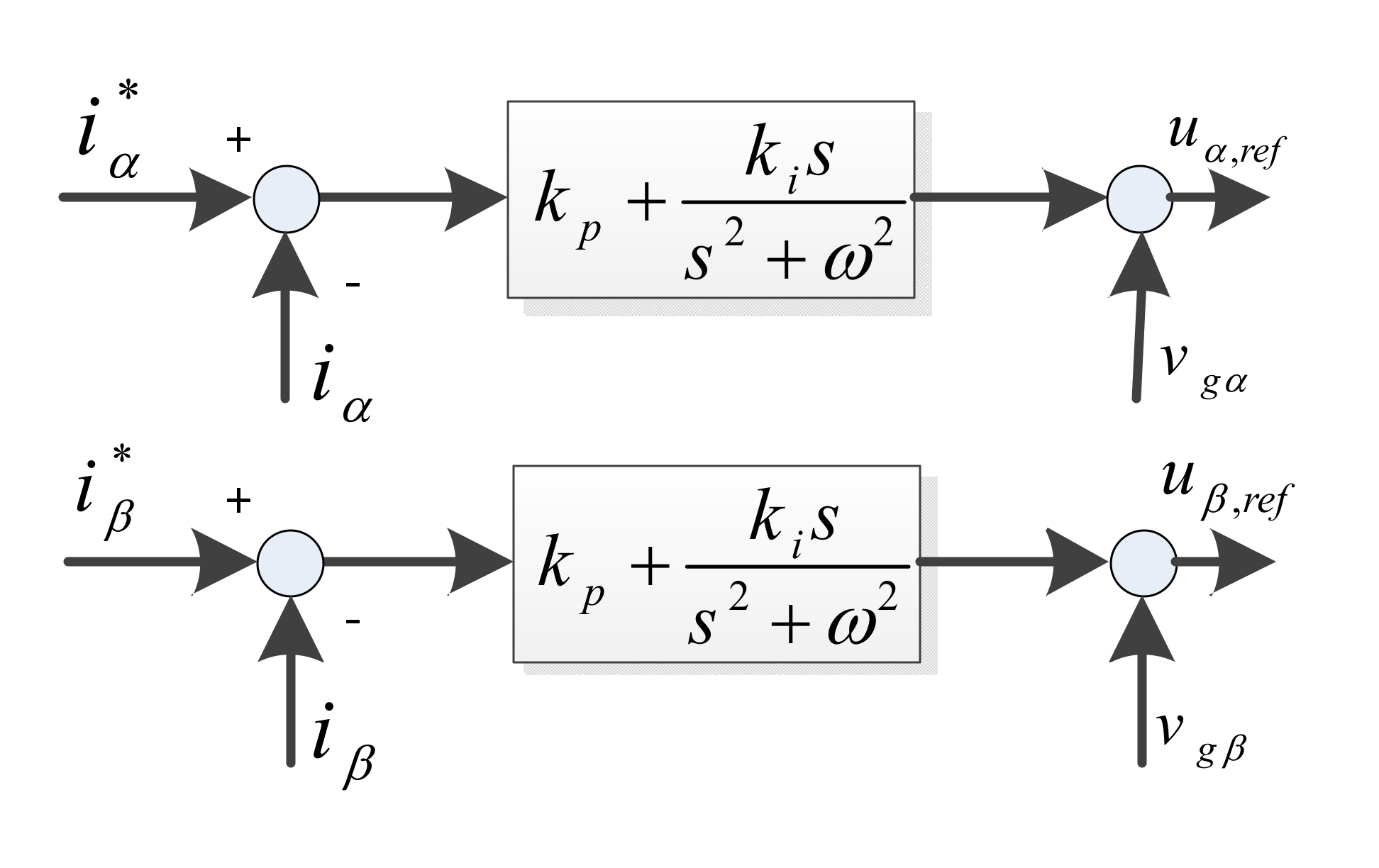
2.3.1. Type I: Ideal PR Controller
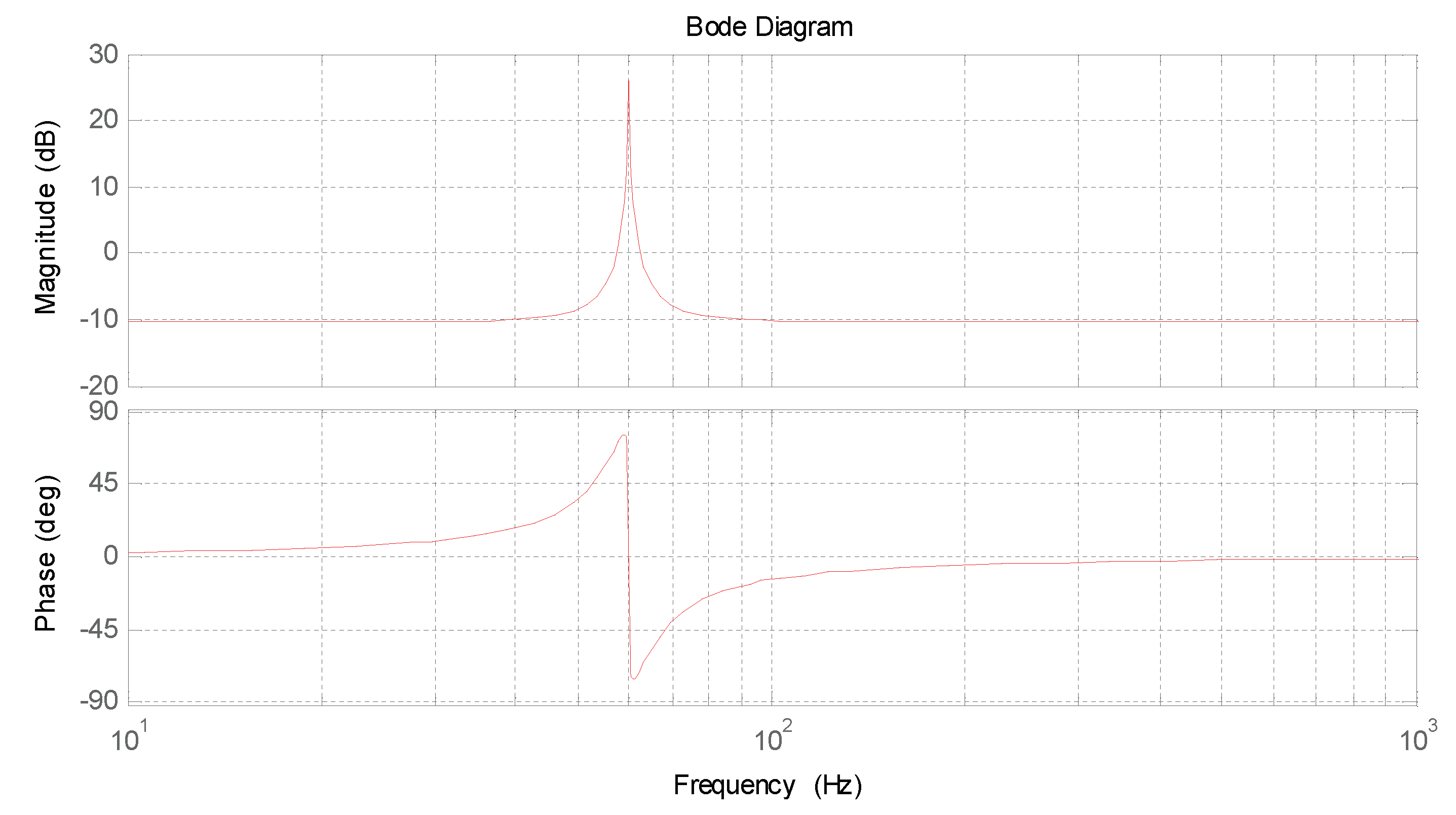
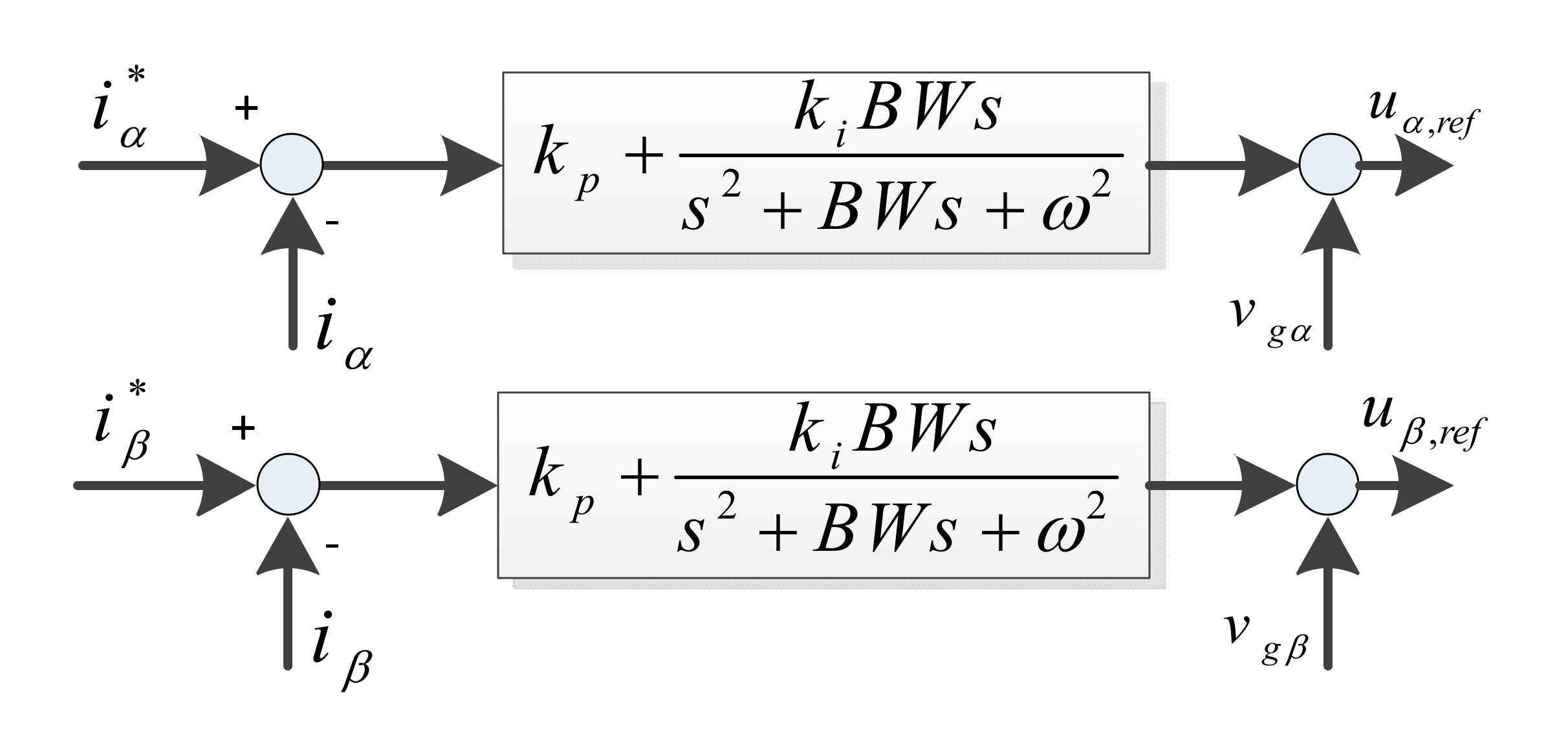
2.3.2. Type II: Non-Ideal PR Controller
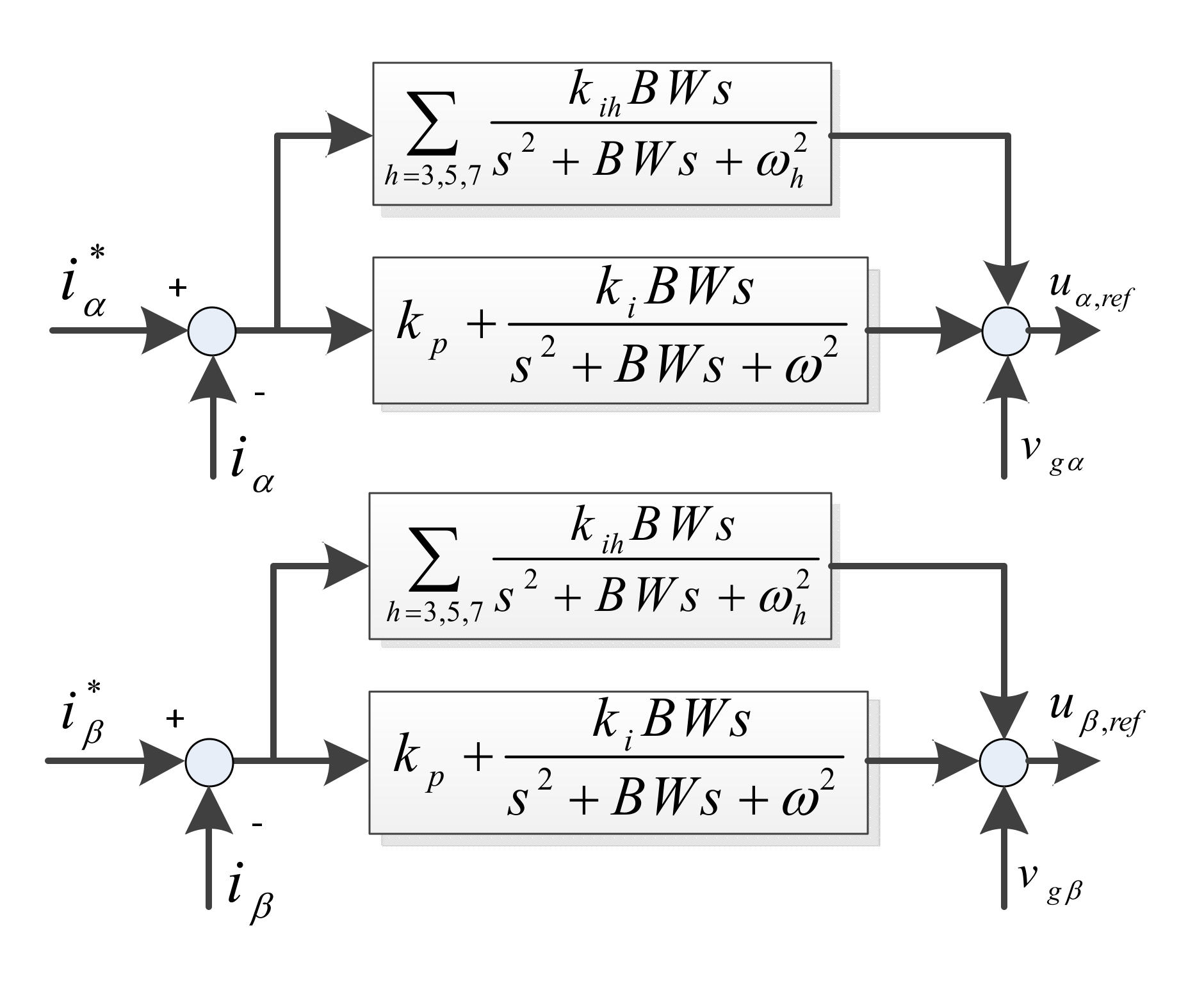
2.3.3. Type III: Non-Ideal PR Controller with a Harmonic Compensators
3. Proposed Power Control Method
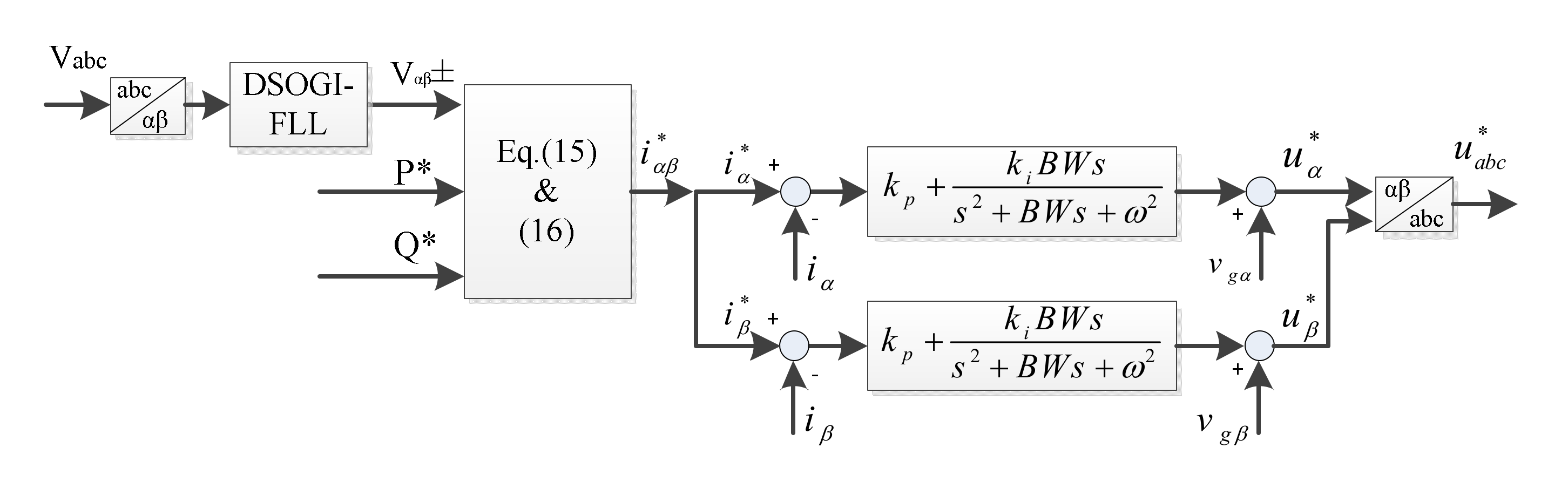
3.1. PNSC
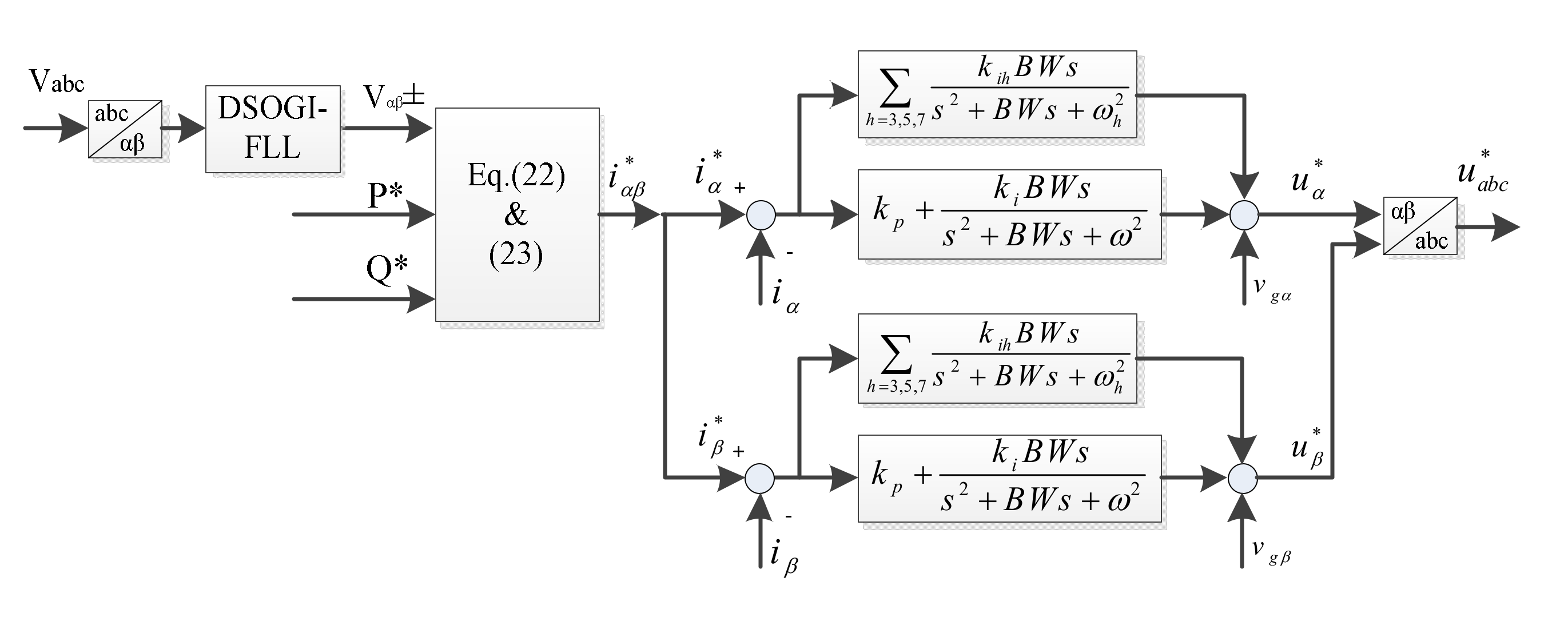
3.2. IARC
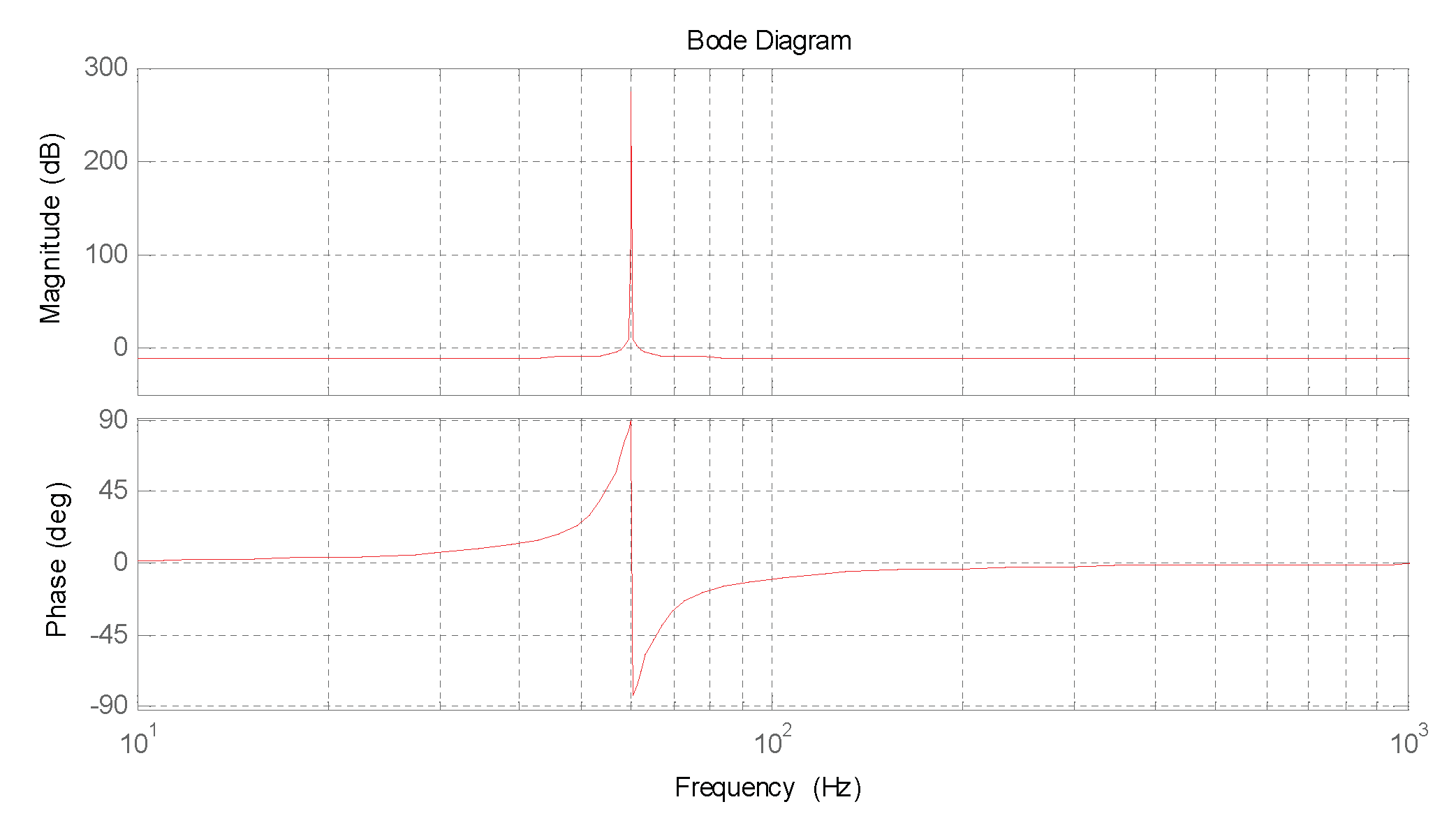
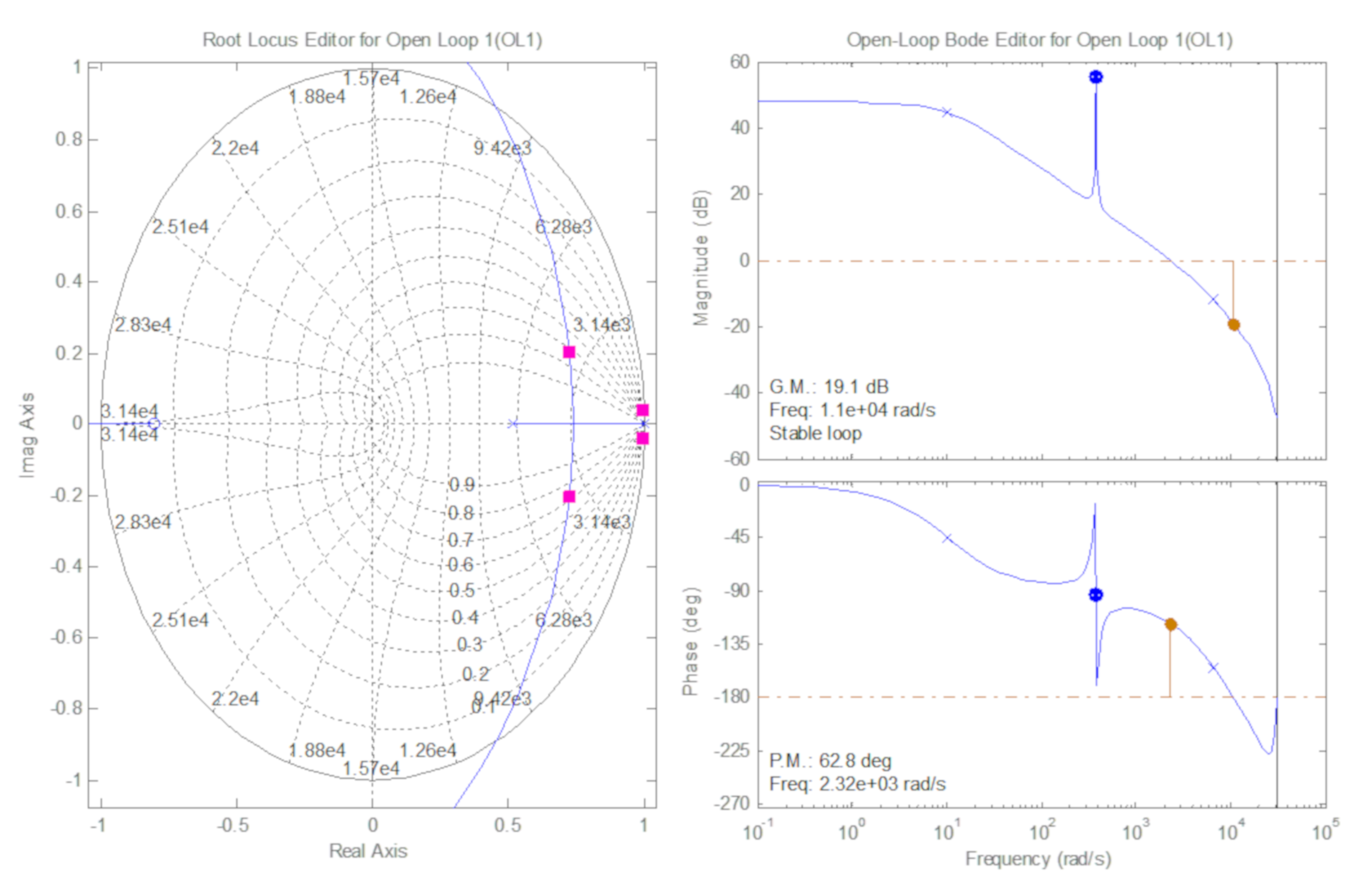
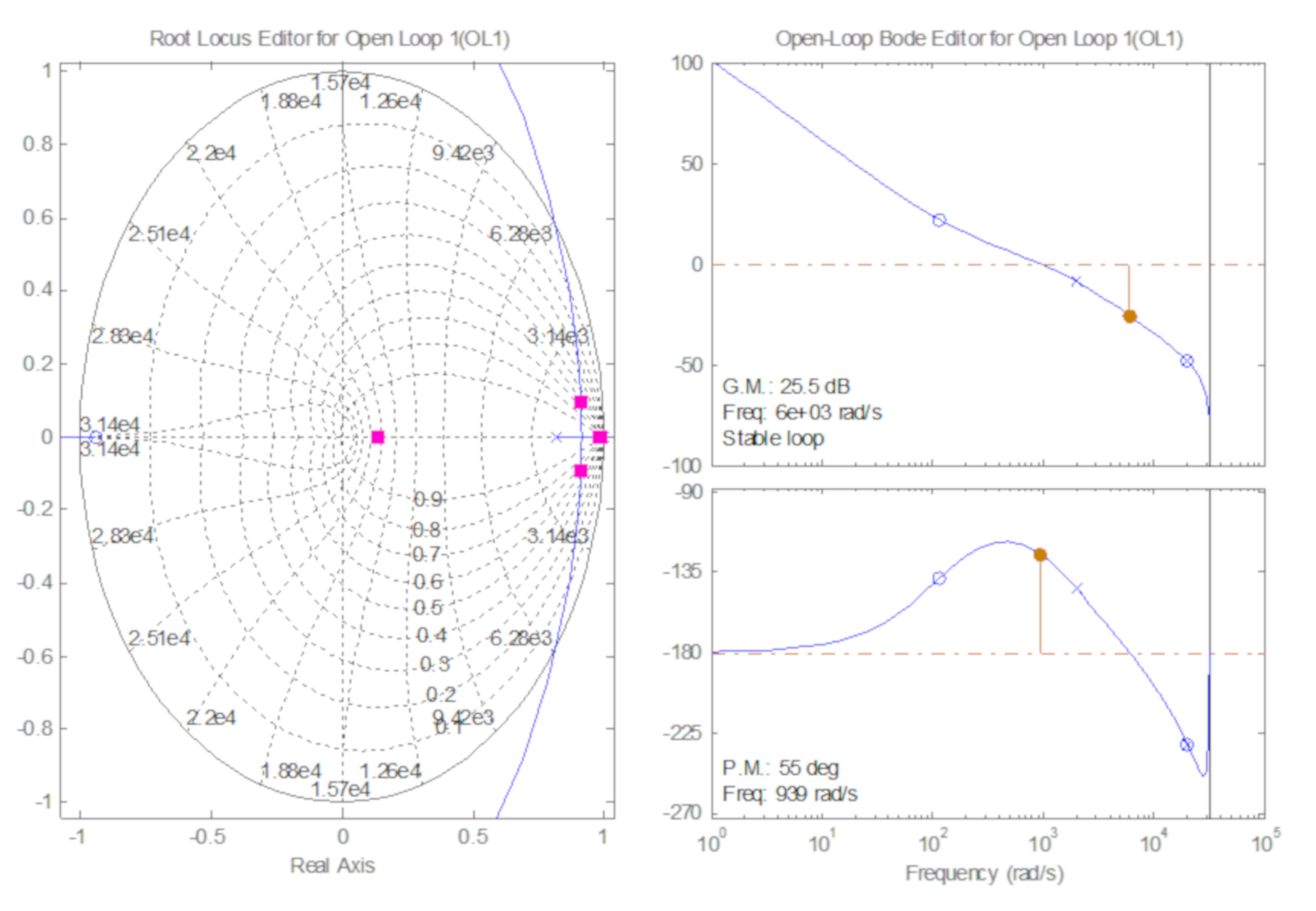
3.3. Controller Design Using Bode Frequency Analysis
4. Simulation Results
4.1. Conventional Current Control Method
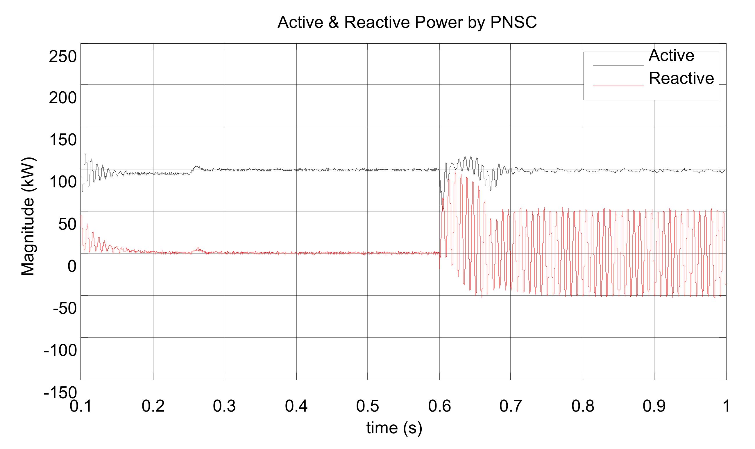
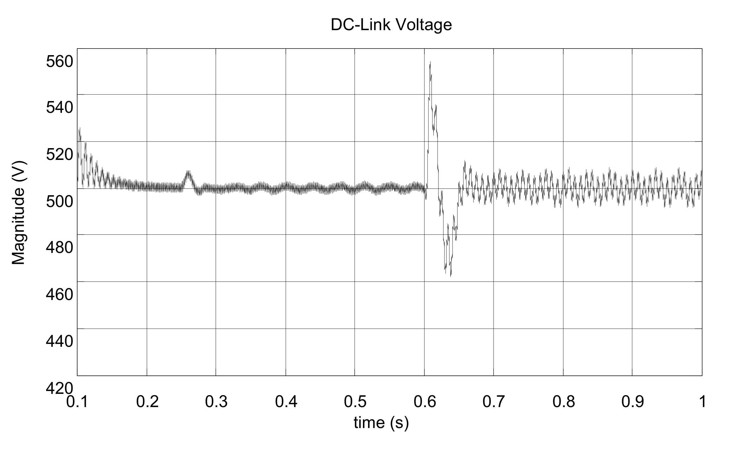
4.2. PNSC Method Performance Using the Type II PR Controller
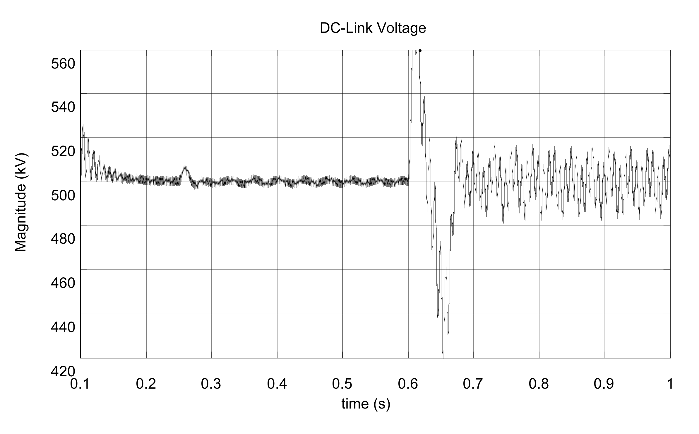
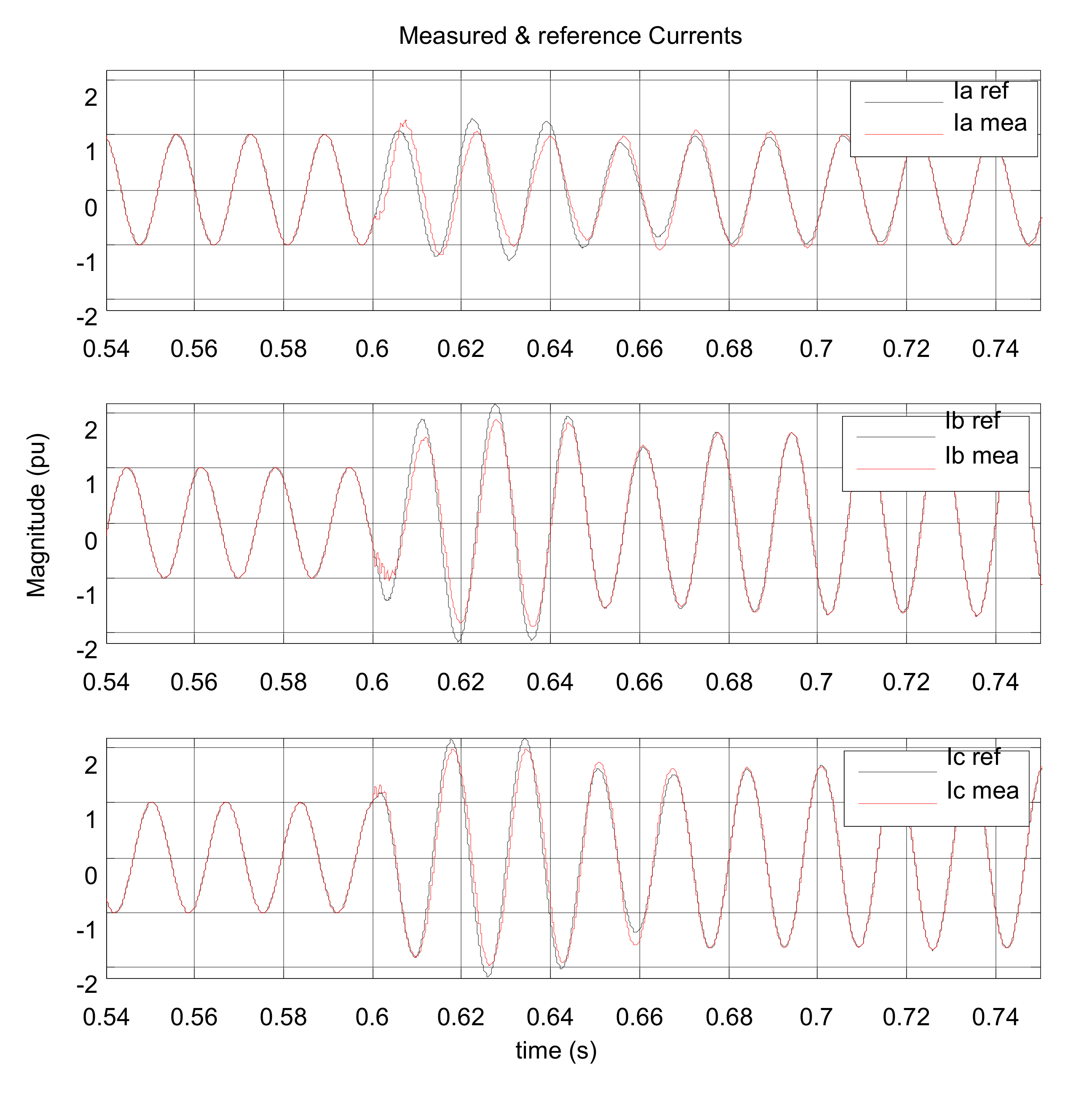
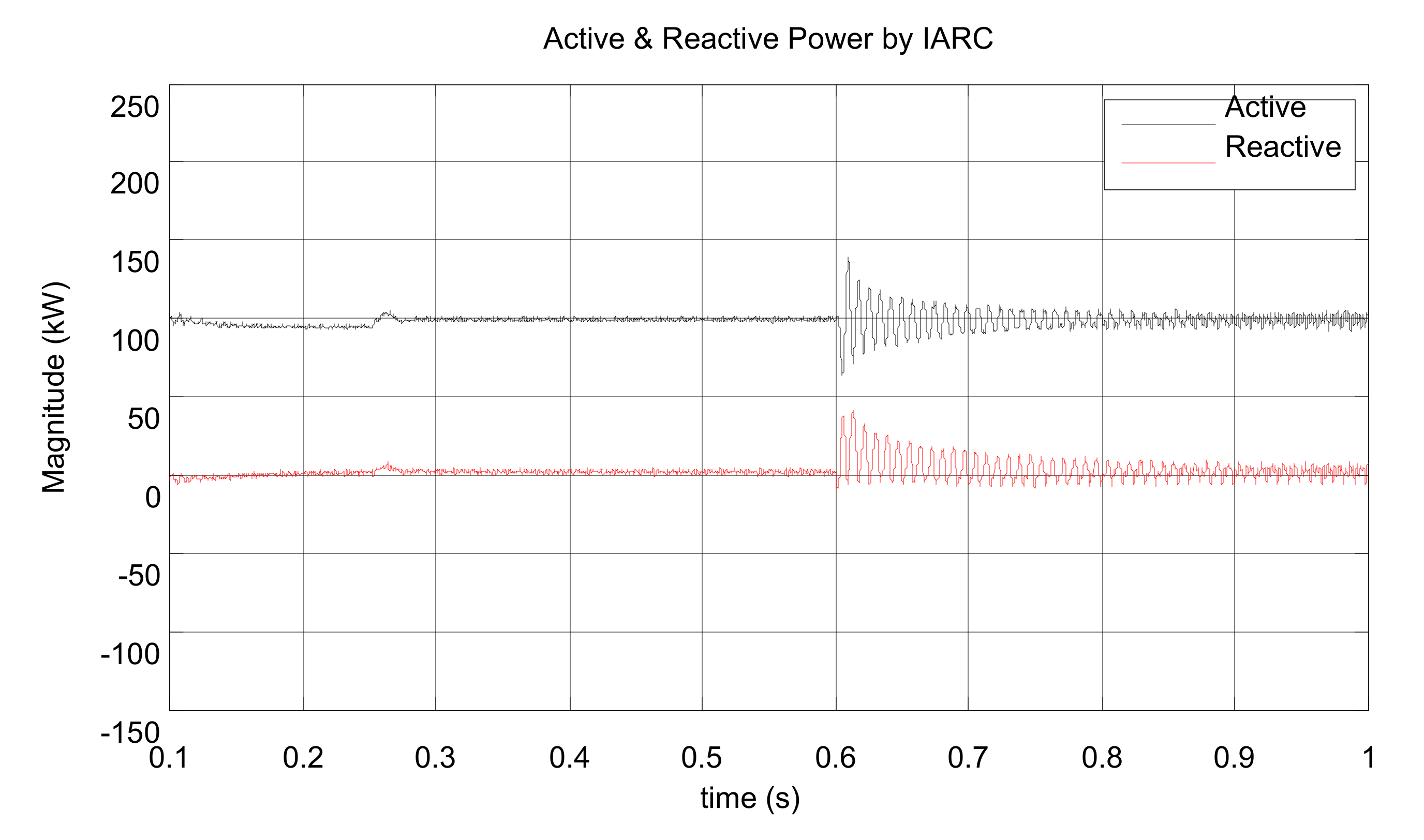
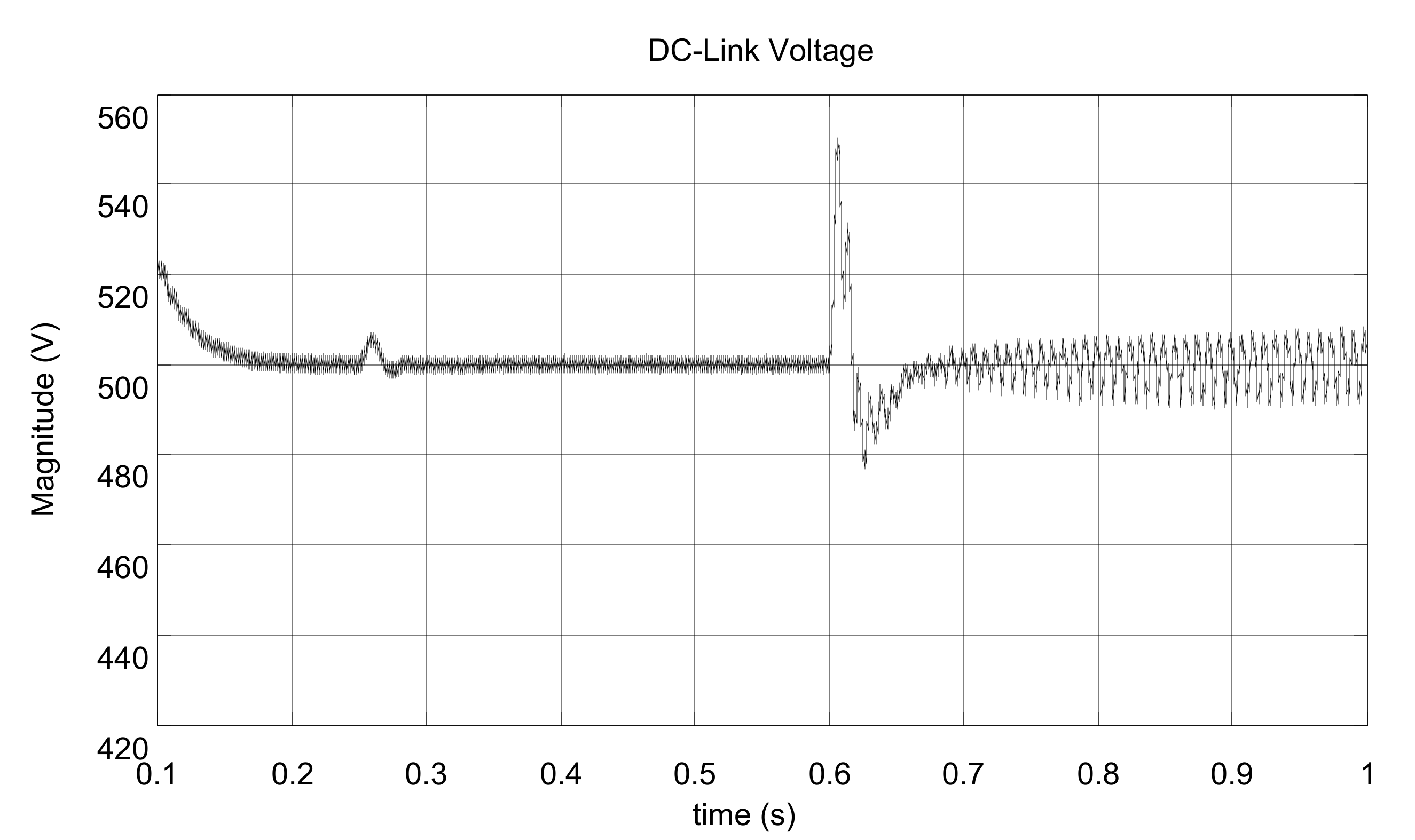
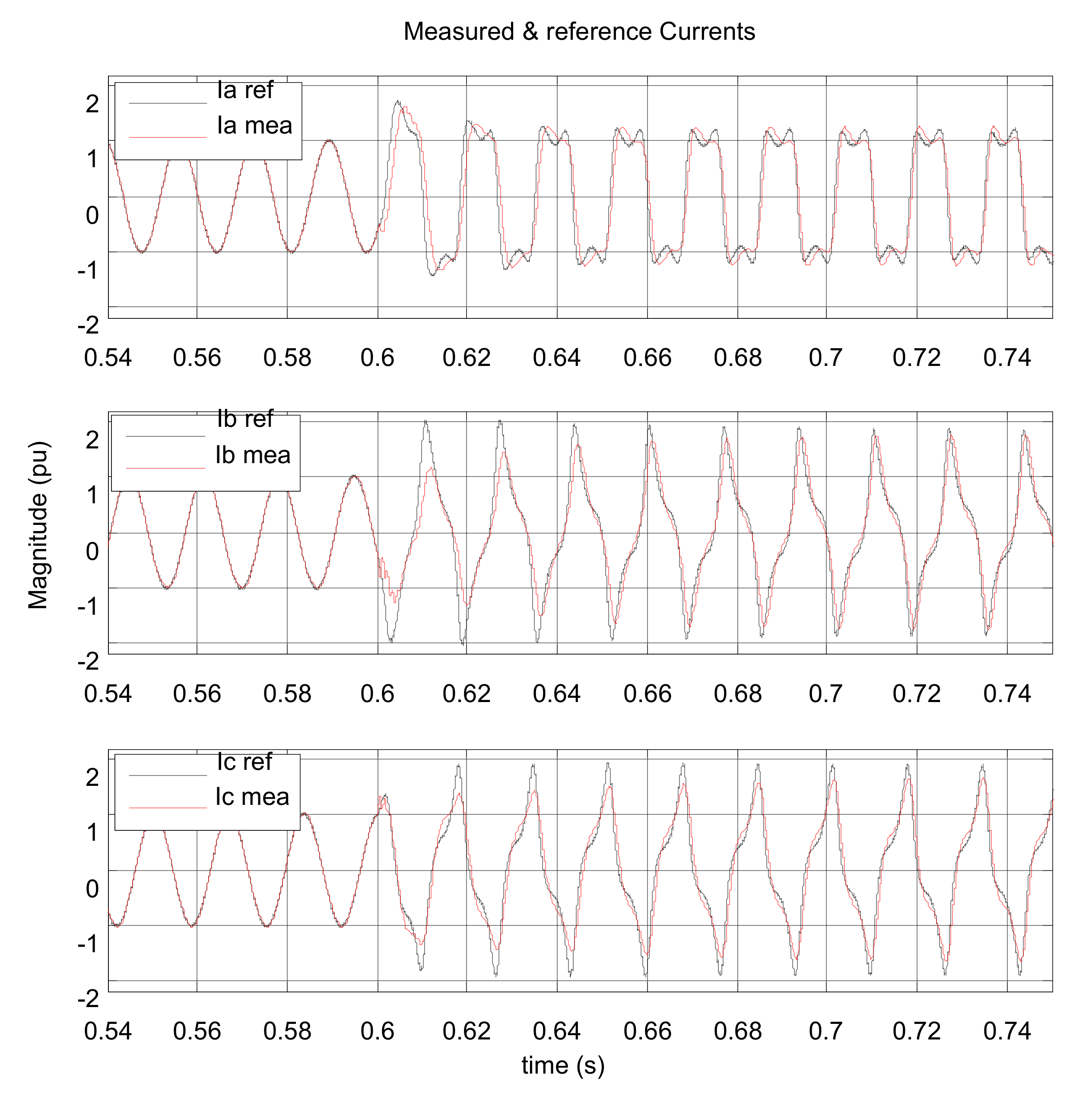
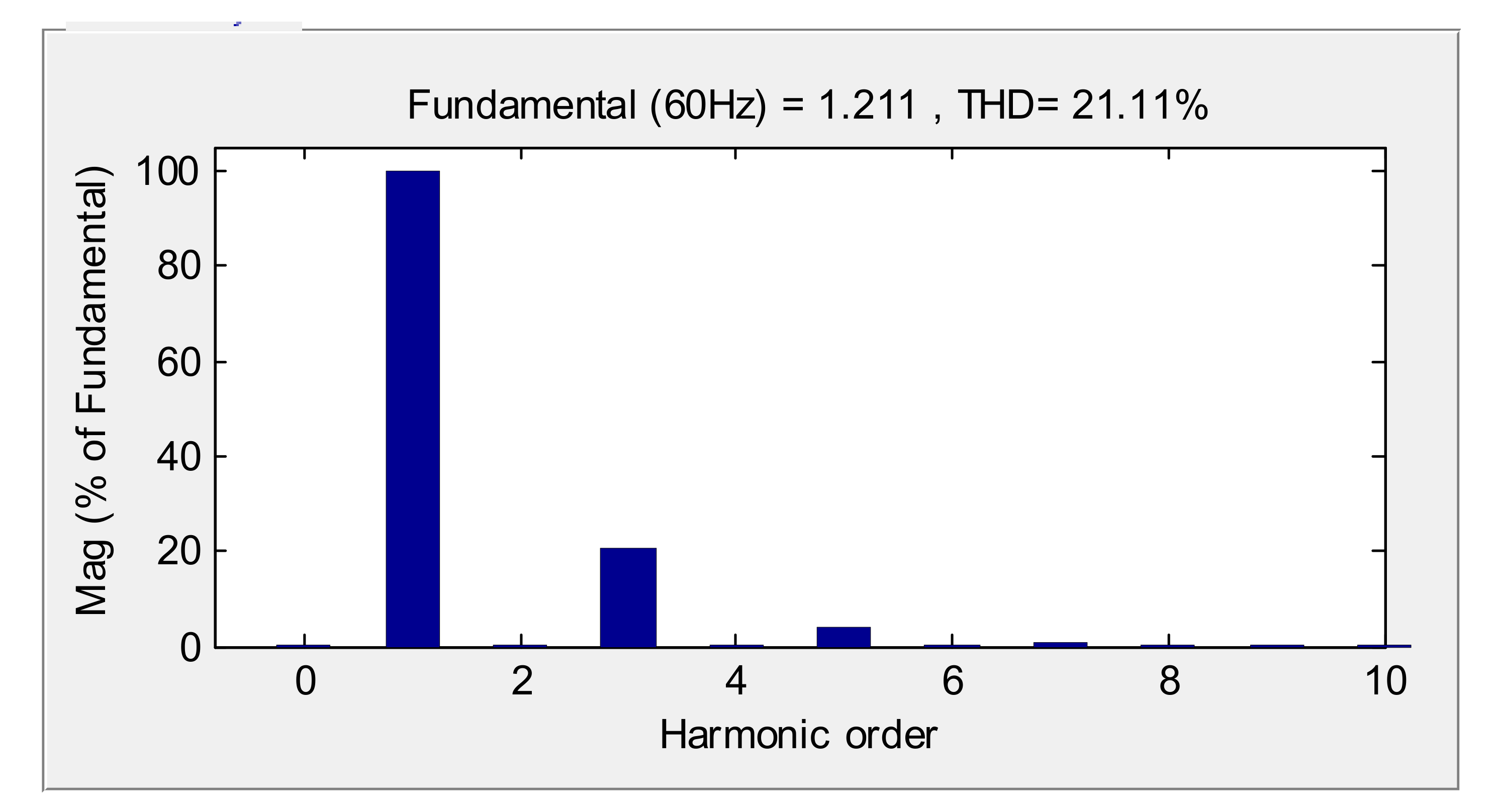
4.3. IARC Method Performance Using the Type III PR Controller
5. Conclusions
Author Contributions
Funding
Conflicts of Interest
Abbreviations
| transfer function of ideal PR controller | |
| proportional gain | |
| integral gain | |
| grid frequency | |
| transfer function of non-ideal PR controller | |
| bandwidth of controller | |
| damping factor | |
| transfer function of non-ideal PR controller with harmonic compensators | |
| orthogonal voltage | |
| constant components of active and reactive power | |
| oscillatory components of active and reactive power | |
| reference current | |
| norm of the grid voltage vector signal | |
| instantaneous conductance | |
| instantaneous susceptance | |
| DC-link capacitance | |
| criteria value of proportional gain | |
| criteria value of integral gain | |
| d component of continuous switching vector | |
| sampling frequency | |
| switching frequency | |
| transfer function of current control loop |
References
- Miveh, M.R.; Mohd, F.G.; Ali, M.M. Control techniques for three-phase four-leg voltage source inverters in autonomous microgrids: A review. Renew. Sustain. Energy Rev. 2016, 54, 1592–1610. [Google Scholar] [CrossRef]
- Shojaei, A.H.; Ghadimi, A.A.; Miveh, M.R.; Mohammadi, F.; Jurado, F. Multi-Objective Optimal Reactive Power Planning under Load Demand and Wind Power Generation Uncertainties Using ε-Constraint Method. Appl. Sci. 2020, 10, 2859. [Google Scholar] [CrossRef]
- Ghadimi, A.A.; Daryani, A.M.; Rastegar, H. Detailed Modeling and analysis of a full bridge PWM DC-DC converter. In Proceedings of the Australasian Universities Power Engineering Conference (AUPEC06), Melbourne, Sydney, Australia, 10–13 December 2006. [Google Scholar]
- Jenniches, S.; Worrell, E. Regional economic and environmental impacts of renewable energy developments: Solar PV in the Aachen Region. Energy Sustain. Dev. 2019, 48, 11–24. [Google Scholar] [CrossRef]
- Mahdavi, M.S.; Gharehpetian, G.B.; Ranjbaran, P.; Azizi, H. Frequency Regulation of AUT Microgrid Using Modified Fuzzy PI Controller for Flywheel Energy Storage System. AUT J. Electr. Eng. 2018, 51, 31–38. [Google Scholar]
- Yilmaz, U.; Kircay, A.; Borekci, S. PV system fuzzy logic MPPT method and PI control as a charge controller. Renew. Sustain. Energy Rev. 2018, 81, 994–1001. [Google Scholar] [CrossRef]
- Tafti, H.D.; Maswood, A.I.; Lim, Z.; Gabriel, O.; Pinkymol, H. A review of active/reactive power control strategies for PV power plants under unbalanced grid faults. In Proceedings of the Innovative Smart Grid Technologies-Asia (ISGT ASIA), Bangkok, Thailand, 4–6 November 2015. [Google Scholar]
- Miveh, M.R.; Mohd, F.G.; Ali, M.M. Power quality improvement in autonomous microgrids using multi-functional voltage source inverters: A comprehensive review. J. Power Electron. 2015, 15, 1054–1065. [Google Scholar] [CrossRef] [Green Version]
- Rezvani, A.; Gandomkar, M. Modeling and control of grid connected intelligent hybrid photovoltaic system using new hybrid fuzzy-neural method. Sol. Energy 2016, 127, 1–18. [Google Scholar] [CrossRef]
- Yang, Y.; Blaabjerg, F.; Wang, H. Low-voltage ride-through of single-phase transformerless photovoltaic inverters. IEEE Trans. Ind. Appl. 2014, 50, 1942–1952. [Google Scholar] [CrossRef] [Green Version]
- Afshari, E.; Moradi, G.R.; Yang, Y.; Farhangi, B.; Farhangi, S. A review on current reference calculation of three-phase grid-connected PV converters under grid faults. In Proceedings of the Power and Energy Conference at Illinois (PECI), Champaign, IL, USA, 23–24 February 2017. [Google Scholar]
- Mirhosseini, M.; Pou, J.; Karanayil, B.; Agelidis, V.G. Positive and negative-sequence control of grid-connected photovoltaic systems under unbalanced voltage conditions. In Proceedings of the Power Engineering Conference (AUPEC), Australasian Universities, Hobart, Australia, 29 September–3 October 2013. [Google Scholar]
- Castilla, M.; Miret, J.; Camacho, A.; Matas, J.; de Vicuña, L.G. Reduction of Current Harmonic Distortion in Three-Phase Grid-Connected Photovoltaic Inverters via Resonant Current Control. IEEE Trans. Ind. Electron. 2013, 60, 1464–1472. [Google Scholar] [CrossRef]
- Dash, A.R.; Babu, B.C.; Mohanty, K.B.; Dubey, R. Analysis of PI and PR Controllers for Distributed Power Generation System under Unbalanced Grid Faults. In Proceedings of the International Conference on Power and Energy Systems (ICPS), Chennai, India,, 22–24 December 2011. [Google Scholar]
- Vidal, A.; Freijedo, F.D.; Yepes, A.G.; Fernandez-Comesana, P.; Malvar, J.; López, Ó.; Doval-Gandoy, J. Assessment and Optimization of the Transient Response of Proportional-Resonant Current Controllers for Distributed Power Generation Systems. IEEE Trans. Ind. Electron. 2013, 60, 1367–1383. [Google Scholar] [CrossRef]
- Teodorescu, R.; Blaabjerg, F.; Liserre, M.; Loh, P.C. Loh Proportional-Resonant Controllers and Filters for Grid-Connected Voltage-Source Converters. IEE Proc. Electr. Power Appl. 2006, 153, 750–762. [Google Scholar] [CrossRef] [Green Version]
- Jiabing, H.; Yikang, H. Modeling and Control of Grid-Connected Voltage-Sourced Converters Under Generalized Unbalanced Operation Conditions. IEEE Trans. Energy Convers. 2008, 23, 903–913. [Google Scholar] [CrossRef]
- Teodorescu, R.; Marco, L.; Pedro, R. Grid Converters for Photovoltaic and Wind Power Systems; John Wiley & Sons: Hoboken, NJ, USA, 2011. [Google Scholar]
- Shao, Z.; Xing, Z.; Fusheng, W.; Renxian, C.; Hua, W. Analysis and control of neutral-point voltage for transformerless three-level PV inverter in LVRT operation. EEE Trans. Power Electron. 2017, 32, 2347–2359. [Google Scholar] [CrossRef]
- Wang, Z.; Bin, W.; Dewei, X.; Ming, C.; Liang, X. Dc-link current ripple mitigation for current-source grid-connected converters under unbalanced grid conditions. IEEE Trans. Ind. Electron. 2016, 63, 4967–4977. [Google Scholar] [CrossRef]
- Guo, X.; Liu, W.; Lu, Z. Flexible power regulation and current-limited control of the grid-connected inverter under unbalanced grid voltage faults. IEEE Trans. Ind. Electron. 2017, 64, 7425–7432. [Google Scholar] [CrossRef]
- Messo, T.; Jokipii, J.; Puukko, J.; Suntio, T. Determining the Value of DC-Link Capacitance to Ensure Stable Operation of a Three-Phase Photovoltaic Inverter. IEEE Trans. Power Electron. 2014, 29, 665–673. [Google Scholar] [CrossRef]
- Yazdani, A.; Dash, P.P. A Control Methodology and Characterization of Dynamics for a Photovoltaic (PV) System Interfaced With a Distribution Network. IEEE Trans. Power Deliv. 2009, 24, 1538–1551. [Google Scholar] [CrossRef]
- Figueres, E.; Garcerá, G.; Sandia, J.; Gonzalez-Espin, F.; Rubio, J.C. Sensitivity Study of the Dynamics of Three-Phase Photovoltaic Inverters With an LCL Grid Filter. IEEE Trans. Ind. Electron. 2009, 56, 706–717. [Google Scholar] [CrossRef] [Green Version]
- Taul, M.G.; Wang, X.; Davari, P.; Blaabjerg, F. An overview of assessment methods for synchronization stability of grid-connected converters under severe symmetrical grid faults. IEEE Trans. Power Electron. 2019, 34, 9655–9670. [Google Scholar] [CrossRef] [Green Version]
- Rodriguez, P.; Luna, A.; Candela, I.; Teodorescu, R.; Blaabjerg, F. Grid synchronization of power converters using multiple second order generalized integrators. In Proceedings of the 34th Annual Conference of IEEE, Orlando, FL, USA, 10–13 November 2008. [Google Scholar]
- Rodriguez, P.; Luna, A.; Etxeberría, I.; Hermoso, J.R.; Teodorescu, R. Multiple Second Order Generalized Integrators for Harmonic Synchronization of Power Converters. In Proceedings of the 2009 Energy Conversion Congress and Exposition ECCE, IEEE, San Jose, CA, USA, 20–24 September 2009. [Google Scholar]
- Wang, Z.; Fan, S.; Zou, Z.; Zheng, Y.; Cheng, M. Operation of interleaved voltage-source-converter fed wind energy systems with asymmetrical faults in grid. In Proceedings of the 7th International Power Electronics and Motion Control Conference (IPEMC), Harbin, China, 2–5 June 2012. [Google Scholar]
- Camacho, A.; Castilla, M.; Miret, J.; Vasquez, J.C.; Alarcón-Gallo, E. Flexible Voltage Support Control for Three-Phase Distributed Generation Inverters Under Grid Fault. IEEE Trans. Ind. Electron. 2013, 60, 1429–1441. [Google Scholar] [CrossRef]
- Rodriguez, P.; Luna, A.; Ciobotaru, M.; Teodorescu, R.; Blaabjerg, F. Advanced Grid Synchronization System for Power Converters under Unbalanced and Distorted Operating Conditions. In Proceedings of the 32nd Annual Conference on IEEE Industrial Electronics, Paris, France, 7–10 November 2006. [Google Scholar]
- Enslin, J.H.R. Maximum power point tracking: A cost saving necessity in solar energy systems. In Proceedings of the 16th Annual Conference of IEEE Industrial Electronics Society, California, CA, USA, 27–30 November 1990. [Google Scholar]
- Esram, T.; Chapman, P.L. Comparison of Photovoltaic Array Maximum Power Point Tr acking Techniques. IEEE Trans. Energy Convers. 2007, 22, 439–449. [Google Scholar] [CrossRef] [Green Version]
- De Brito, M.A.G.; Galotto, L.; Sampaio, L.P.; e Melo, G.D.A.; Canesin, C.A. Evaluation of the Main MPPT Techniques for Photovoltaic Applications. IEEE Trans. Ind. Electron. 2013, 60, 1156–1167. [Google Scholar] [CrossRef]
- Zmood, D.N.; Holmes, D.G. Stationary frame current regulation of PWM inverters with zero steady state error. In Proceedings of the 30th Annual IEEE Power Electronics Specialists Conference, Charleston, SC, USA, 1 July 1999. [Google Scholar]
- Cha, H.; Vu, T.K.; Kim, J.E. Design and control of Proportional-Resonant controller based Photovoltaic power conditioning system. In Proceedings of the Energy Conversion Congress and Exposition, California, CA, USA, 20–24 September 2009. [Google Scholar]
- Monfared, M.; Golestan, S. Control strategies for single-phase grid integration of small-scale renewable energy sources: A review. Renew. Sustain. Energy Rev. 2012, 16, 4982–4993. [Google Scholar] [CrossRef]
- Julean, A.M. Active Damping of LCL Filter Resonance in Grid Connected Applications. Master’s Thesis, Aalborg University, Aalborg, Denmark, 2009. [Google Scholar]
- Liserre, M.; Dell’Aquila, A.; Blaabjerg, F. Design and control of a three-phase active rectifier under non-ideal operating conditions. In Proceedings of the 37th IAS Annual Meeting Industry Applications Conference, Pittsburgh, PA, USA, 13–18 October 2002. [Google Scholar]
- Liserre, M.; Blaabjerg, F.; Hansen, S. Design and control of an LCL-filter-based three-phase active rectifier. IEEE Trans. Ind. Appl. 2005, 41, 1281–1291. [Google Scholar] [CrossRef]


| Symbol | Quantity | Nominal Value |
|---|---|---|
| QSG gain | ||
| proportional gain of DC-link controller | ||
| integral gain of DC-link controller | ||
| proportional gain of current control | ||
| integral gain of current control | ||
| integral gain of current control 3th harmonic compensator | ||
| integral gain of current control 5th harmonic compensator | ||
| integral gain of current control 7th harmonic compensator | ||
| Damping factor of PR controller |
| Quantity | Nominal Value |
|---|---|
| Maximum output power | 100 kW |
| Switching frequency | 3 kHz |
| Maximum power PV output voltage | 500 V |
| DC-link capacitor | 9 μF |
| Inverter side inductance | 250 μH |
| Inverter side parasitic resistance | 2 mΩ |
| Filter capacitor | 45 μF |
| Filter damping resistance | 0.6 Ω |
| Grid side inductance | 220 μH |
| Grid side parasitic resistance | 2.7 mΩ |
| Grid interfaced transformer voltage | 260 V/25 kV |
| Grid frequency | 60 Hz |
| Sampling frequency | 10 kHz |
| Q reference | 0 VAr |
| Harmonic Orders | Values Based on a Percentage of the Fundamental Frequency |
|---|---|
© 2020 by the authors. Licensee MDPI, Basel, Switzerland. This article is an open access article distributed under the terms and conditions of the Creative Commons Attribution (CC BY) license (http://creativecommons.org/licenses/by/4.0/).
Share and Cite
Abbasi, S.; Ghadimi, A.A.; Abolmasoumi, A.H.; Reza Miveh, M.; Jurado, F. Enhanced Control Scheme for a Three-Phase Grid-Connected PV Inverter under Unbalanced Fault Conditions. Electronics 2020, 9, 1247. https://doi.org/10.3390/electronics9081247
Abbasi S, Ghadimi AA, Abolmasoumi AH, Reza Miveh M, Jurado F. Enhanced Control Scheme for a Three-Phase Grid-Connected PV Inverter under Unbalanced Fault Conditions. Electronics. 2020; 9(8):1247. https://doi.org/10.3390/electronics9081247
Chicago/Turabian StyleAbbasi, Saeid, Ali Asghar Ghadimi, Amir Hossein Abolmasoumi, Mohammad Reza Miveh, and Francisco Jurado. 2020. "Enhanced Control Scheme for a Three-Phase Grid-Connected PV Inverter under Unbalanced Fault Conditions" Electronics 9, no. 8: 1247. https://doi.org/10.3390/electronics9081247