Atmospheric Responses to Mesoscale Oceanic Eddies in the Winter and Summer North Pacific Subtropical Countercurrent Region


1
Physical Oceanography Laboratory/CIMST and Ocean-Atmosphere Interaction and Climate Laboratory, Ocean University of China and Qingdao National Laboratory for Marine Science and Technology, Qingdao 266100, China
2
Department of Atmospheric Sciences, Texas A&M University, College Station, TX 77840, USA
*
Author to whom correspondence should be addressed.
Atmosphere 2020, 11(8), 816; https://doi.org/10.3390/atmos11080816
Submission received: 17 July 2020
/
Revised: 31 July 2020
/
Accepted: 1 August 2020
/
Published: 3 August 2020
(This article belongs to the Section Meteorology)
Abstract
:In the winter and summer North Pacific Subtropical Countercurrent region, the atmospheric responses to 20,000+ mesoscale oceanic eddies (MOEs) are examined using satellite and reanalysis data from 1999 to 2013. The composite results indicate that surface wind speed, cloud, and precipitation anomalies are positively correlated with sea surface temperature anomalies in both seasons. The surface wind speed anomalies and convective precipitation anomalies show dipolar structures centering on MOEs in winter and on unipolar structures in summer. In both seasons, the vertical mixing mechanism plays an obvious role in the atmospheric responses to MOEs. In addition, the distributions of sea level pressure anomalies in winter reflects the effects of the pressure adjustment mechanism. Due to the seasonal variations in the atmospheric background state and the MOEs, the sensitivities of surface wind speeds, clouds, and precipitation responses to MOEs in summer are over 30% higher than those in winter.
1. Introduction
Mesoscale oceanic eddies (MOEs) with lifetimes of 4~52 weeks and diameters of 50~400 km, which play an important role in ocean circulations as well as heat and mass transports, constitute a crucial part of the mesoscale characteristics of oceans [1,2,3]. The horizontal and vertical movement of sea water in MOEs can cause sea surface temperature anomalies (SSTAs), and the mesoscale air–sea interactions associated with MOEs are rooted in the SSTAs caused by MOEs [4].
Two mechanisms have been proposed to explain the influences of mesoscale SSTAs caused by MOEs on the atmosphere. The pressure adjustment mechanism [5] suggests that warm (cold) water could increase (decrease) sea level pressure. The second one is the vertical mixing mechanism [6,7,8,9], wherein static stability is weakened (enhanced) over warm (cold) water, resulting in intensifying (weakening) of turbulence mixing within the marine atmospheric boundary layer (MABL). Consequently, the increased (decreased) downward momentum transport accelerates (decelerates) the surface wind over warm (cold) water, which accounts for 13–15% of the atmospheric variability in the Southern Ocean [10,11]. Under strong background wind conditions, the vertical mixing mechanism plays a more dominate role in changing the wind speed, while weaker background wind is more favorable for the pressure adjustment mechanism [11,12].
The SSTAs caused by MOEs can also affect cloud cover and local precipitation [4]. Ma et al. (2015) [13] examined atmospheric responses to 35,000+ MOEs in the Kuroshio Extension (KE) region by using satellite and reanalysis data. The results indicated that the MOEs-induced cloud and precipitation anomalies were 3.6% and 7.5% of the background values, respectively. In addition, field observations and numerical experiments showed that MOEs affect the development of clouds over them [14,15,16]. The vertical mixing and pressure adjustment mechanisms generate wind divergence anomalies, modifying the vertical motion and thus influencing the clouds and precipitation. When the dynamic mechanism dominate, the cloud and precipitation anomalies correspond to the large value regions of sea surface temperature (SST) gradients. A second mechanism is the thermal effect attributed to changes in heat and moisture transportation caused by the SSTAs, and the cloud, precipitation and SST anomalies are in-phase. The second mechanism is more apparent in the existing research results [10,13].
The MOEs in the North Pacific, characterized by strong eddy kinetic energy (EKE) [17], are prevalent in the KE region and subtropical countercurrent (STCC) region (Figure 1a). Through previous analyses of satellite data, reanalysis data, observation data and numerical simulation results, the existing literature has elucidated the atmospheric responses to the MOEs in the KE region [12,13,14,15,18,19]. In the STCC region, by analyzing satellite data, Chow and Liu (2013) [20] found that there were phase differences between the centers of SSTAs and the centers of MOEs in the spring, while the surface wind speed anomalies (SWSAs) pattern bears a discernable resemblance to the SSTAs pattern. The SWSAs induced by SSTAs had a corresponding distribution. Xu et al. (2018) [21] explored the coupling between MOEs and the atmosphere when SSTAs and SWSAs are in negative phase in the STCC region in summer. The deeper mixed layers in warm eddies restrict the cooling in the tropical cyclone centers in the STCC region, which contribute to the maintenance and development of tropical cyclones [22,23,24,25]. Since there are few studies on the atmospheric responses to the MOEs in the STCC region (particularly compared to the KE region), significant gaps in our knowledge remain regarding the extent and seasonal variations of atmospheric responses.
There are obvious seasonal variations in the oceanic and atmospheric background conditions in the STCC region, casting doubt on whether the different background states can have an impact on the MOEs modulating the atmosphere. Therefore, the objectives of this study are: first, to examine the influences of MOEs on the atmosphere in different seasons; second, to investigate the underlying physical mechanisms. To explore the aforementioned problems, we examine the atmospheric responses to 20,000+ MOEs in the winter and summer STCC regions using satellite and reanalysis data. Composite analyses and filtering are used to quantify the effects of the MOEs.
2. Data and Methods
2.1. Data
The location and amplitude data of MOEs in this study are from the MOEs database established through MOE detection using sea surface height data [2]. The scopes of MOEs are determined using the sea surface height anomaly (SSHA) data provided by archiving, validation and interpretation of satellite oceanographic data (AVISO) with a horizontal resolution of 0.25° × 0.25° [26]. The edge of an MOE is the isoline whose sea surface height difference from the center of the MOE is the amplitude of the MOE.
We also use the SST and cross calibrated multi-platform (CCMP) 10-m wind field data provided by remote sensing systems (REMSS). The SST, wind field, column-integrated cloud liquid water content and precipitation data were obtained from the tropical rainfall measuring mission’s (TRMM) microwave imager (TMI) [27], and the sea surface flux data are from the Japanese ocean flux with use of remote sensing observations (J-OFURO) version 3 dataset [28]. The horizontal resolution of the above data is 0.25° × 0.25°.
In addition to satellite data, the climate forecast system reanalysis (CFSR) and climate forecast system version 2 (CFSv2) 6-hourly reanalysis data were also employed in this study. The horizontal resolution of sea surface data is 0.313° × 0.313°, and the resolution of pressure level data with 37 layers is 0.5° × 0.5° [29].
2.2. Methods
Due to the different available periods and resolutions of the selected data, we selected the period of 1999–2013 in which all data are available for composite analyses, and can be interpolated to 0.25° × 0.25° and daily data. We use the Student’s t test to evaluate the statistical significance of the composite analyses.
MOEs with a diameter smaller than 50 km in the study area are eliminated, on account of the relatively coarse data resolution. At the same time, in order to ensure the statistical significance of the results, only the MOEs with amplitude in the upper 50th percentile are included in the composite analyses. Each eligible MOE in the area studied in each day is treated as an independent eddy. Then, we collocate oceanic and atmospheric variables with the composite area of a box of 6° latitude by 6° longitude centered relative to each eddy center. A total of 4205 cyclonic eddies (CEs) and 3934 anticyclonic eddies (AEs) were selected in winter, and 6164 CEs and 6378 AEs were selected in summer. More MOEs occur in summer with larger EKE. To obtain the anomalies of each variable potentially influenced by MOEs, each variable is zonally high-pass filtered using a cut-off wavelength of 1000 km [1,30,31]. This zonal high-pass filter effectively removes seasonal cycles and other variations with scales larger than 1000 km [19].
3. Results
3.1. Oceanic and Atmospheric Background Conditions
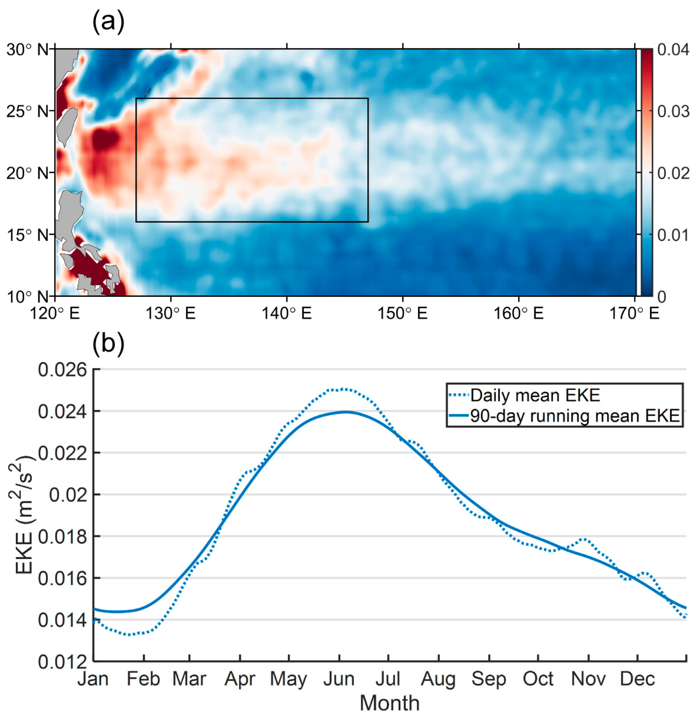
The area studied in this paper is located in the area of higher EKE in the western portion of the STCC region (black box in Figure 1a, 16°~26° N, 127°~147° E, which is away from land as required by the filtering method). The mean EKE in the study area was 0.014 m2 s−2 in winter (November to January) and 0.022 m2 s−2 in summer (June to August) (Figure 1b). The summertime increase in mean EKE agrees with the findings of Qiu et al. (2014) [16]. However, the SST gradients in winter were notably larger (Figure 2). In terms of atmospheric background fields, the stronger (weaker) sea level pressure (SLP) gradients in winter (summer) led to prevailing northeast (southeast) winds of 6 m s−1 (2 m s−1).
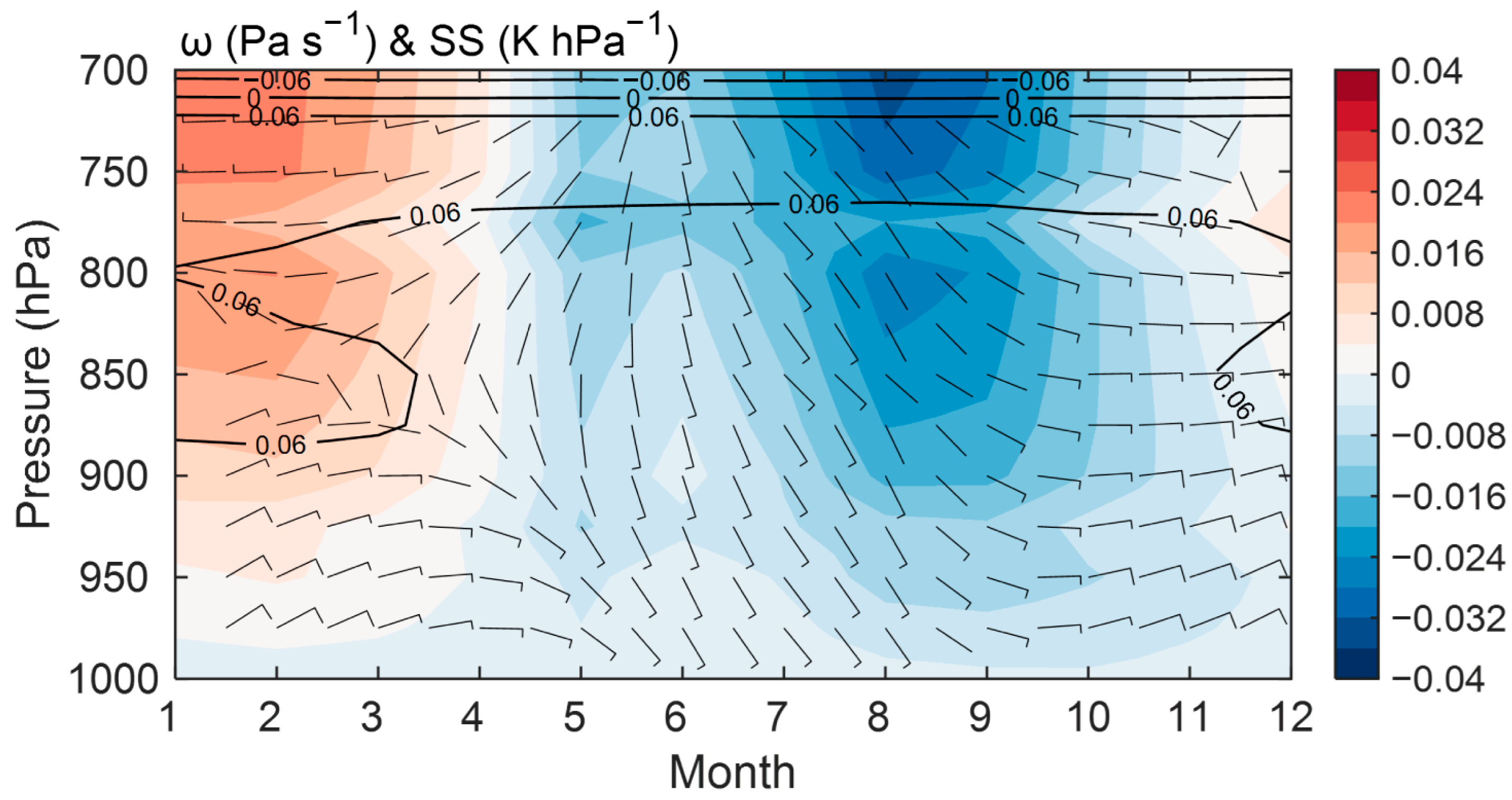
The vertical gradient of potential temperature (i.e., static stability) shows that the average depth of the MABL in the study area was about 850 hPa in winter and 750 hPa in summer (Figure 3). In winter (summer), the mean wind speed was about 4 m s−1 (2 m s−1) in the MABL, accompanied with downward (upward) motion. Wood et al. (2006) [32] proposed that the stability of the MABL can be measured by the estimated inversion strength (EIS). The mean EIS in winter (7.77 K) was greater than that in summer (4.96 K), so the MABL in winter was more stable than in summer. Considering the distinct seasonal variations in the oceanic and atmospheric background state, we supposed that such variations may cause different atmospheric responses to MOEs in winter and summer. Therefore, the data in winter and summer were selected for separate composite analyses to explore the seasonal variations in atmospheric responses to MOEs in the following study.
3.2. Atmospheric Responses to MOEs in Winter and Summer
3.2.1. Surface Wind Speed
Figure 4 shows the distributions of SSTAs near MOEs and the scope of MOEs composited by satellite data. The mean amplitude of CEs (AEs) was 13.9 cm (12.9 cm) in winter and 14.9 cm (15.4 cm) in summer. In the summer with larger EKE, MOEs were more active and their mean amplitude was slightly larger. However, the SSTAs caused by MOEs in winter were about 2.7 times those in summer. The phase differences between the minimum (maximum) of SSTAs and the CEs (AEs) centers in winter (CEs: 49.1°; AEs: 55.4°) were larger than in summer (CEs: 36.0°; AEs: 32.7°). SSTAs were shifted west from SSHAs, which is consistent with eddies in the South Indian Ocean, South Pacific Ocean, South China Sea and STCC region [1,19,33,34].
The impacts of MOEs on SSTAs were mainly driven by two processes: the horizontal thermal advection caused by MOE circulation and the vertical thermal advection attributed to the rise and fall associated with MOEs [33,35]. Due to the larger background meridional SST gradient in winter, the horizontal thermal advection by counterclockwise (clockwise) circulations of CEs (AEs) was amplified, more likely producing SSTAs on both sides of MOEs. This is consistent with the aforementioned greater phase differences in winter than in summer.
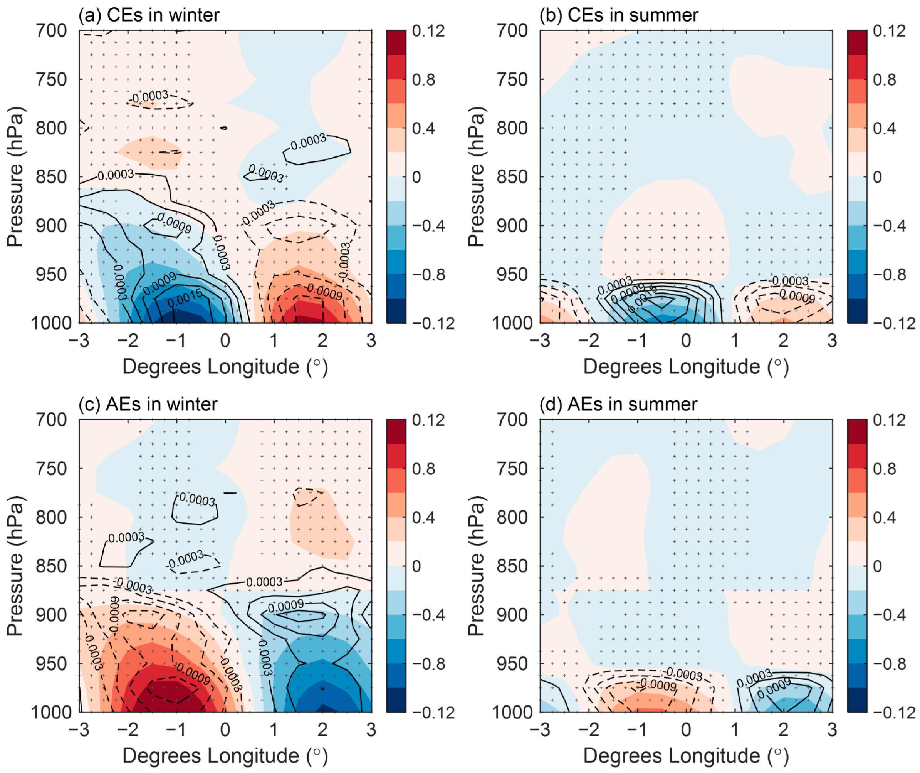
SSTAs associated with MOEs affect the lower atmosphere by changing the near-surface turbulent heat fluxes [36,37,38]. Under the background condition of SST with higher than surface air temperatures, when the SSTA is negative (positive), the turbulent heat flux anomaly is downward (upward), and less (more) heat is transferred to the atmosphere from the sea. The spatial distributions of turbulent heat flux anomalies correspond well with the spatial distributions of SSTAs, which reflects the instantaneous response of turbulent heat fluxes [10] and the effects of SSTAs on air–sea energy exchanges (Figure 5 and Figure 6). In addition, the air temperature over MOEs changes under the influence of such energy exchanges. When the SST is abnormally low (high), the air temperature is abnormally low (high), and the MABL becomes more stable (unstable) (Figure 7). In winter, the static stability anomalies extend higher (Figure 7a,c), reaching 850 hPa, while they are below 950 hPa in summer (Figure 7b,d), and the intensities of two seasons are similar.
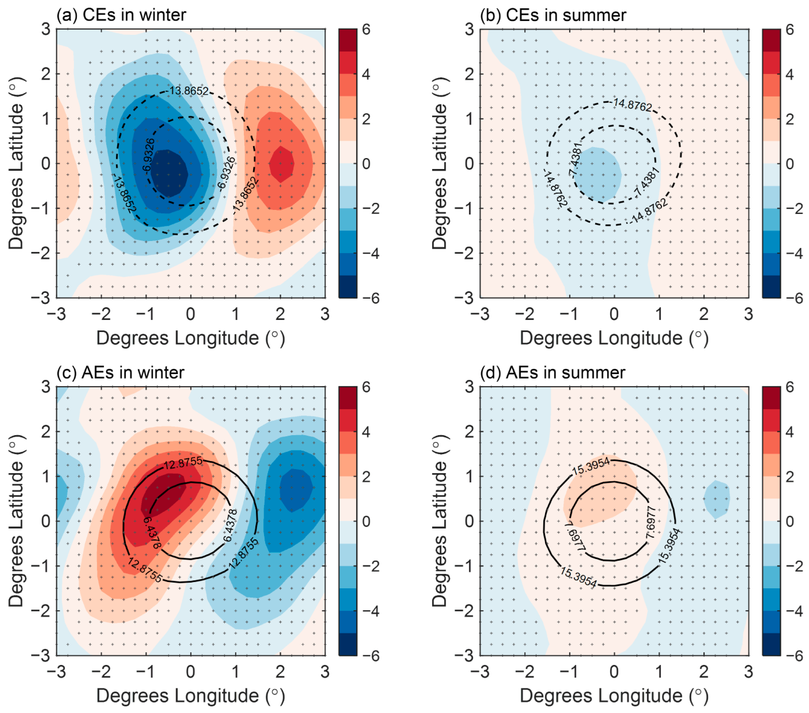
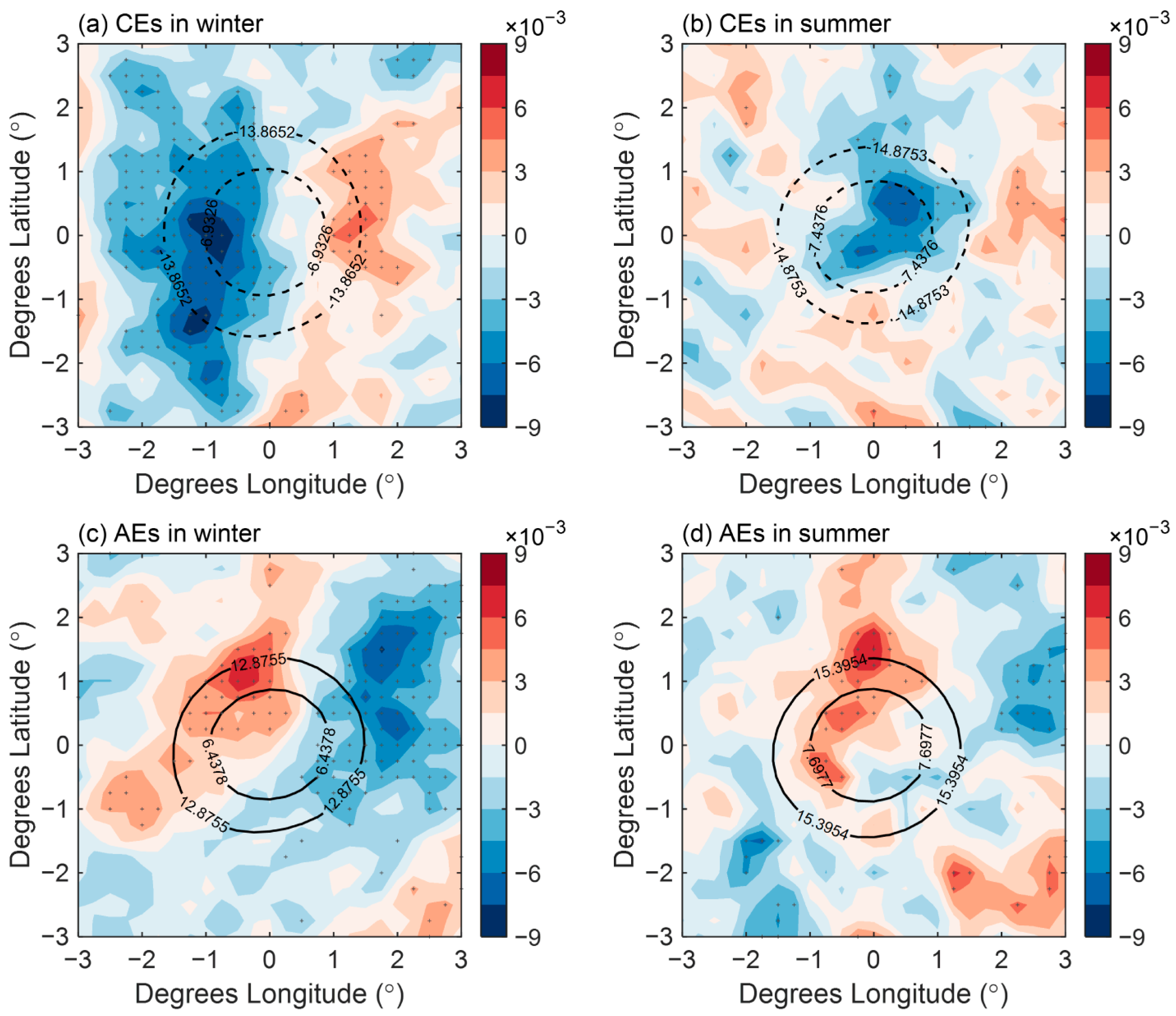
According to previous studies, changes in atmospheric stability over the MOEs are supposed to modulate the turbulent mixing and related downward momentum transport, thus leading to modifications of surface wind speeds. The wind response process is completed within about an hour [9]. As depicted in Figure 8, the distributions of SWSAs are analogous to the distributions of SSTAs. Where the SST is abnormally low (high), the MABL becomes more stable (unstable), the turbulence mixing is weakened (intensified), and the surface wind magnitude decreases (increases), which we ascribe to the vertical mixing mechanism [5,6,7]. In winter, the phase differences between SWSAs’ and MOEs’ centers are large (CEs: 54.0°; AEs: 69.2°), and the distributions of SWSAs are nearly a dipole relative to MOEs’ center, whereas in summer, the phase differences are small (CEs: −13.9°; AEs: −16.4°), and the SWSAs display a clear unipolar pattern (Figure 8). The intensities of the SWSAs are similar in winter and summer, corresponding to 1.9% and 2.6% of the background surface wind speed, respectively.
The vertical mixing mechanism is expressed as a linear correlation between the wind divergence perturbation to the downwind SST gradient [17,39]. We examined the linear relationship between them by binning the wind divergence perturbations to downwind SST gradients and averaged thereafter [9,34]. The bin sizes are of 5 × 10⁻⁴ °C km−1 and the spacing for SST gradients was smaller and larger than |5 × 10⁻³ °C km−1|. The results showed that the vertical mixing mechanism played an important role in the atmospheric responses to MOEs, both in winter (correlation coefficient: 0.988) and in summer (correlation coefficient: 0.984).
3.2.2. Sea Level Pressure
MOEs can not only affect the surface wind speed through the vertical mixing mechanism, but also influence the SLP via the pressure adjustment mechanism [3,7,40]. In winter, the SLP anomalies showed a dipolar structure centering on the MOEs with an amplitude of 2 Pa (Figure 9a,c). Conversely, the summer SLP anomalies’ distributions were not very clear, and the anomalies were below 0.8 Pa (Figure 9b,d). The pressure adjustment mechanism is expressed as a linear correlation between wind divergence to the Laplacian of the SST field [39]. Their correlation coefficient was 0.945 in winter and 0.108 in summer. This discrepancy indicates that the pressure adjustment mechanism plays a relatively large role in the atmospheric response to MOEs in winter, but not in summer.
3.2.3. Clouds and Precipitation
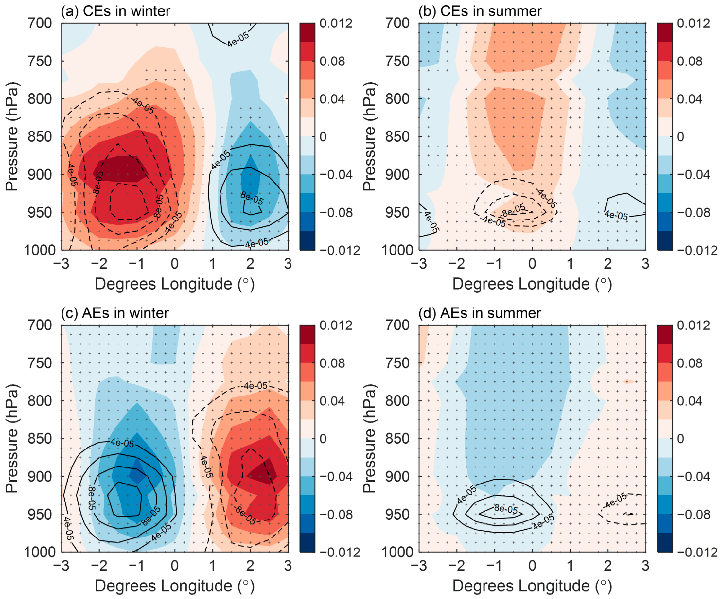
The MOE-caused SSTAs and associated latent heat flux anomalies described above lead to changes in moisture in the MABL. Figure 10 shows that the specific humidity in the MABL clearly responds to SSTAs. The cold (warm) SSTAs decreased (increased) moisture, with slightly greater responses in winter. In addition, the ω anomalies over the cold (warm) sea surface were downward (upward), which shows the effects of MOEs on the air vertical motion (Figure 10). Although the SSTAs were weak in summer, the ω anomalies could reach higher (over 700 hPa). However, in winter, the lower MABL height and higher background static stability limited the upward propagations of atmospheric vertical motion anomalies.
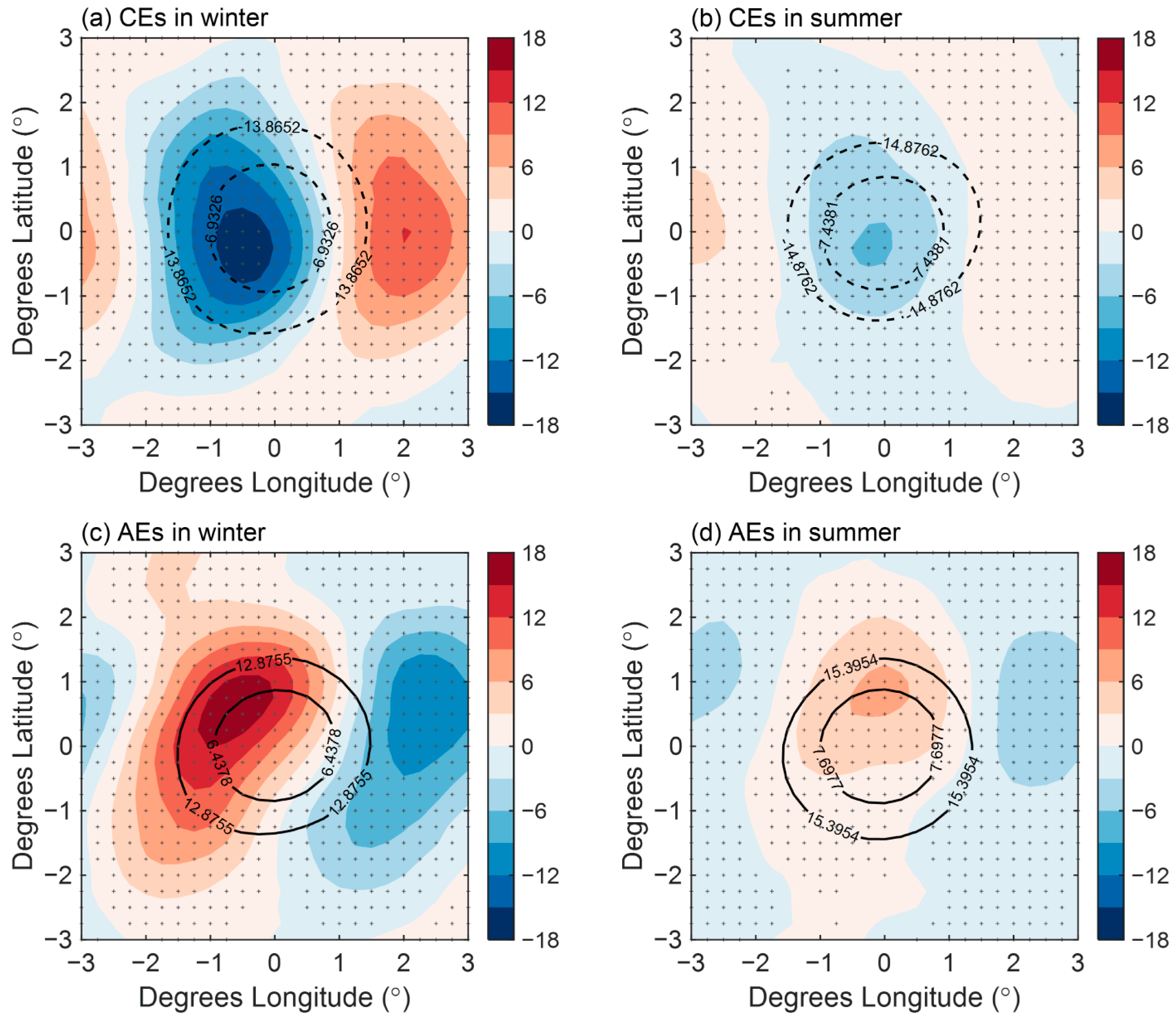
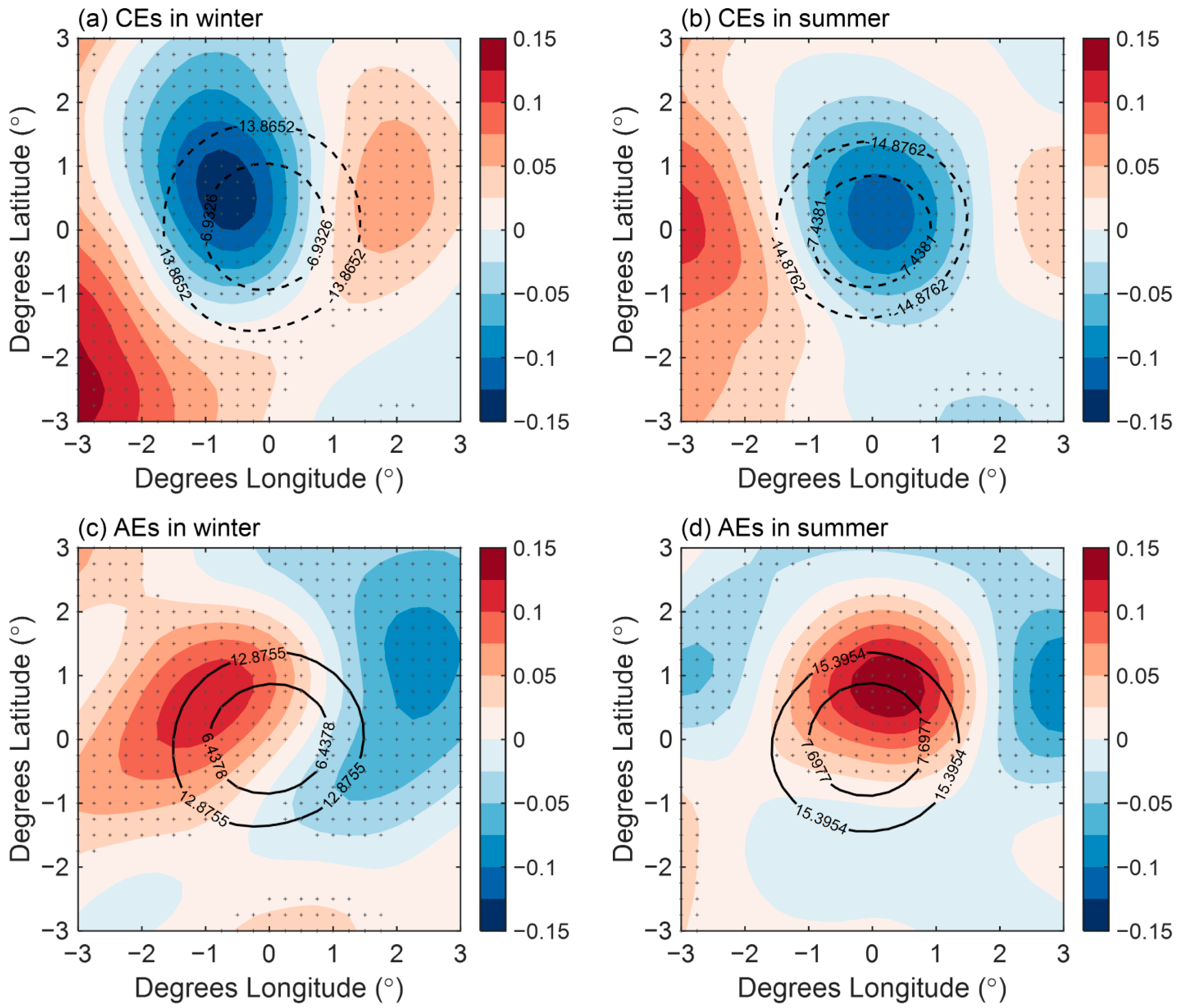
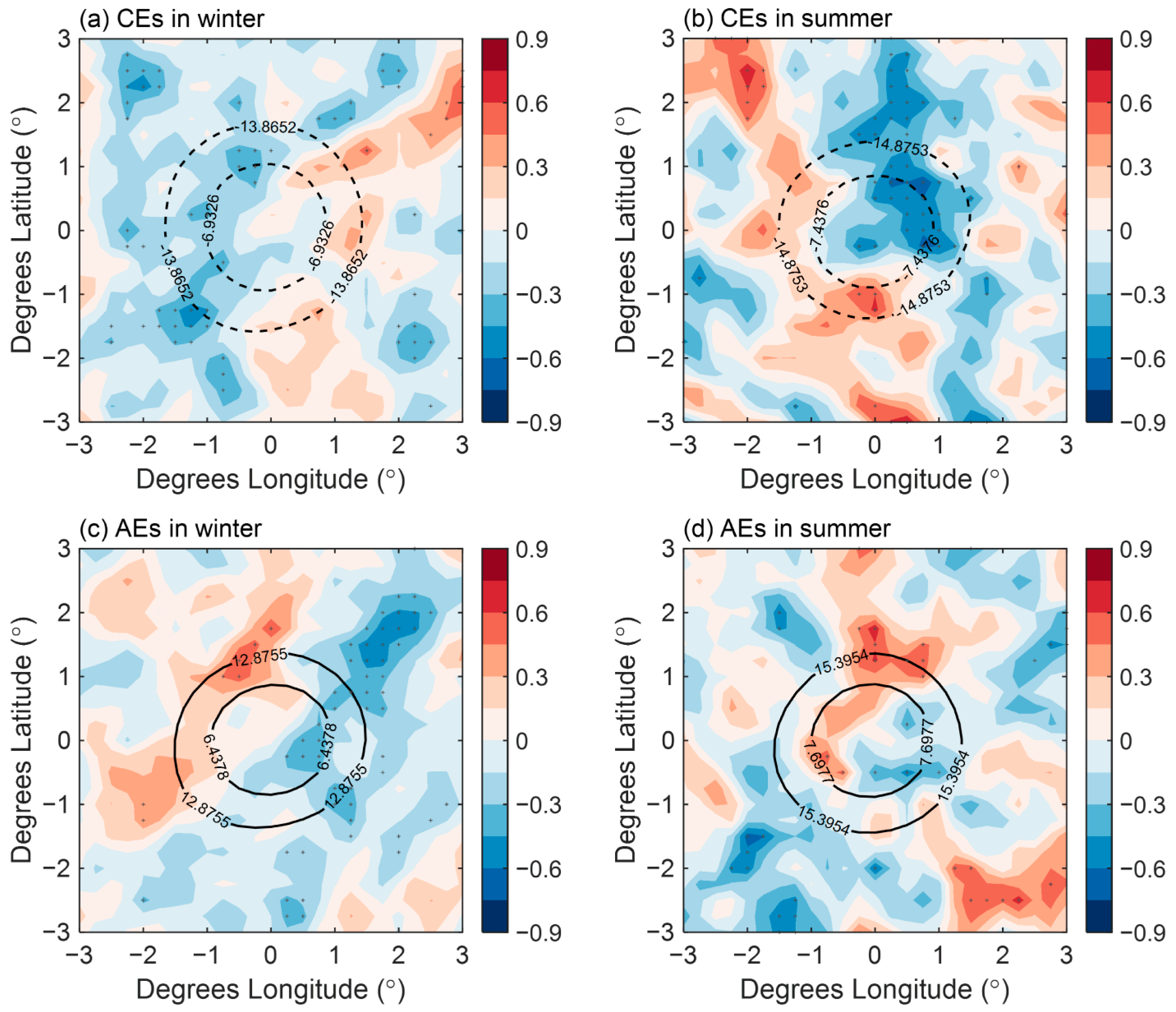
As shown above, MOEs can influence the moisture and vertical motion of the lower atmosphere, and consequently clouds and precipitation also respond to MOEs [9,12]. In winter, the anomalies of cloud liquid water (Figure 11a,c) and total precipitation (Figure 12a,c) were distributed on both sides of the MOEs, and their intensities were 9.0% and 20.8% of the background values, respectively. In summer, the anomalies were relatively concentrated in the MOEs’ center (Figure 11b,d and Figure 12b,d), and their intensities were 7.8% and 17.3% of the background values. The cloud and precipitation anomalies corresponded to the heat fluxes anomalies, indicating that the thermal mechanism plays an important role.
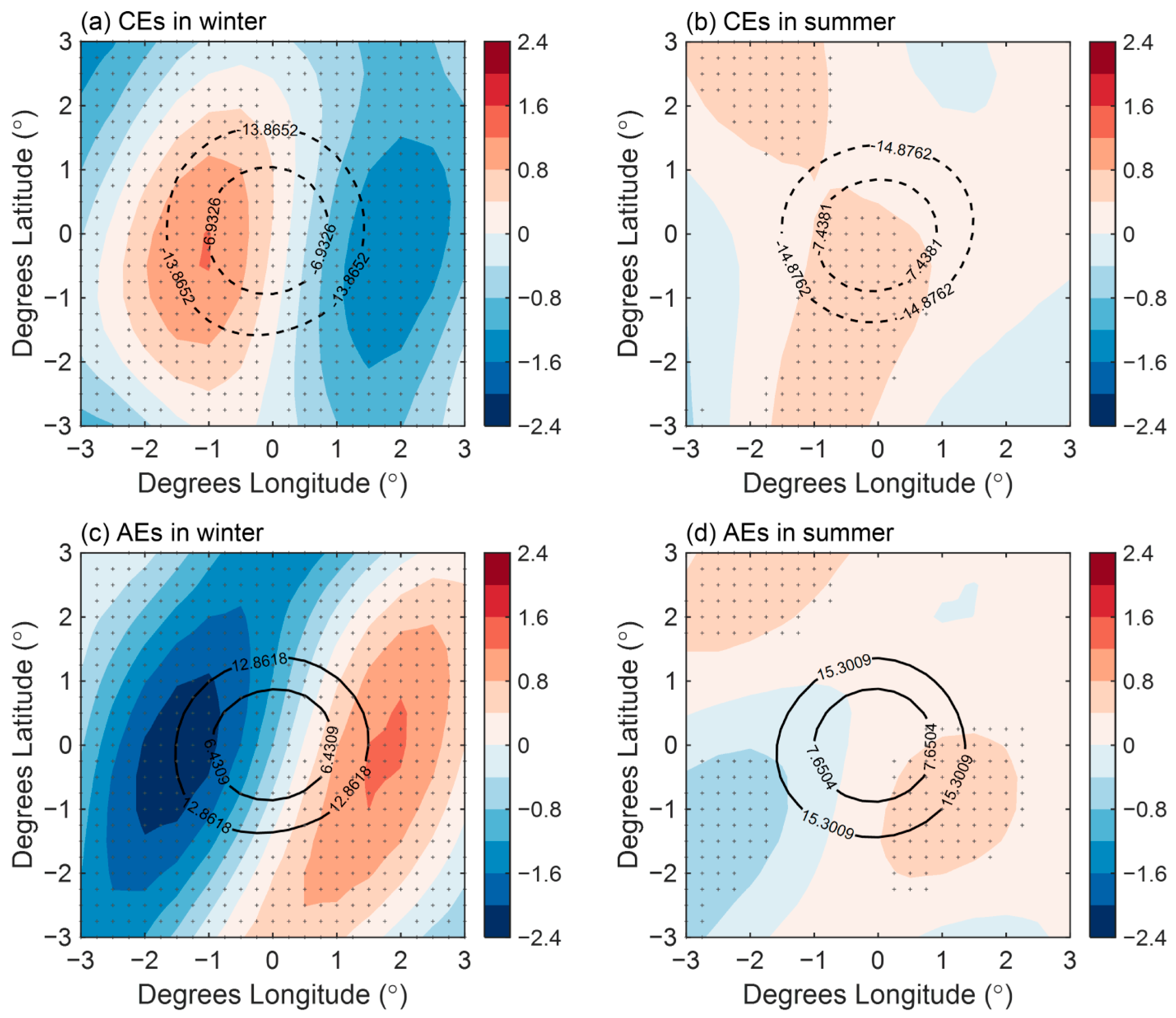
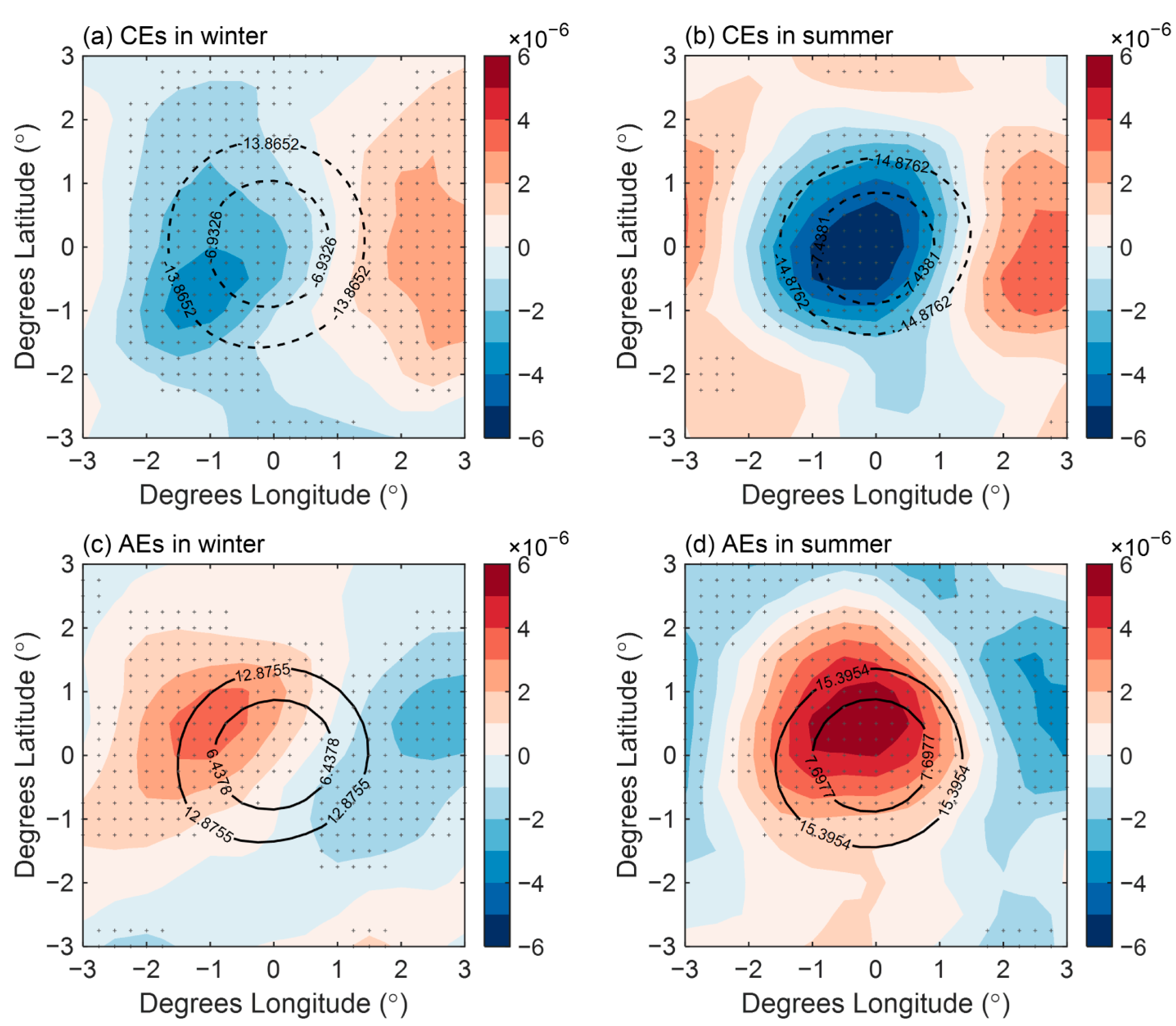
We also analyzed convective precipitation anomalies, which are closely related to local moisture and vertical motion. As shown in Figure 13, convective precipitation anomalies were more significant and the intensities of the anomalies were stronger in summer, about 1.7 times those in winter. By contrast, large-scale precipitation had no significant anomalies (figure omitted).
3.2.4. Sensitivities of Atmospheric Responses
Through composite analyses, we found that the MOEs-associated SSTAs in winter were about 2.7 times those in summer, but the wind speed anomalies induced by MOEs in winter and summer were similar (Figure 8), and the convective precipitation anomalies in summer were even greater than those in winter (Figure 13). We also composited CFSR data and TMI data, and found that the results were consistent with the composite results above.
To give quantitative estimates of the atmospheric imprints induced by MOEs, linear fits were made to SST-q anomaly scatterplots, where q is another variable [12,34]. The significance of the fits was assessed using the t test. We still used the binning here. The bin sizes were of 0.05 °C spacing for SST gradients smaller and larger than |0.5 °C|. The slopes of linear fits to SSTAs for all the variables are summarized in Table 1. The slopes of SSTAs and turbulent heat flux were larger in winter than in summer, which may be related to the larger surface wind speeds in winter. However, the slopes of SSTAs and SWSAs were 40% more in summer than in winter. In the STCC region, the MABL was more unstable in summer than in winter, and the unstable MABL could promote stronger responses of wind speed to the MOEs [34,41]. In addition, through the analysis of the relationship between sea surface wind divergence and SST, we found that both the vertical mixing mechanism and pressure adjustment mechanism played a role in the process of atmospheric response in winter. Therefore, the circulation anomalies brought by the adjusted air pressure anomalies will also have an impact on the wind fields, which may also lead to the weakening of the slope of SSTAs and SWSAs in winter.
The responses of clouds and precipitations to the MOEs were also more sensitive in summer. The slopes of SSTAs and cloud liquid water anomalies were about 30% more in summer than in winter. The slope of SSTAs and total precipitation anomalies was 10% more in summer in TMI data, but the slope in summer was more than three times the slope in winter in CFSR data. This may be due to the strong responses of convective precipitations in summer in CFSR data. In the study area, there was more moisture in the MABL, and the MABL was more unstable and dominated by ascending motion, with better conditions for convective precipitation in summer. Under this background, the increase (decrease) of moisture in the atmospheric boundary layer induced by MOEs and the upward (downward) vertical movement anomalies are more likely to trigger (inhibit) convective precipitation.
4. Discussion and Conclusions
In this study, we focused on the atmospheric responses to MOEs in the STCC region in summer and winter and compared the discrepancies between them. We used composite analyses and filtering to investigate the responses of several atmospheric variables and the underlying mechanisms. Based on the results of composite analyses, we found that the response sensitivities of surface wind speeds, clouds and precipitations in summer were over 30% higher than those in winter. Specific conclusions are:
- (1)
- The MOEs in the STCC region can affect the atmosphere, particularly surface wind speed, MABL stability, clouds and precipitation. In the investigated period, the phase differences between the SSTA maximum/minimum and MOEs’ centers in winter were greater than those in summer, which led to similar distributions of turbulent flux anomalies, MABL stability anomalies, specific humidity anomalies and ω anomalies. Furthermore, the SWSAs and convective precipitation anomalies near the MOEs displayed dipolar distributions on both sides of the MOEs in winter and unipolar distributions in the center of MOEs in summer.
- (2)
- In winter, both the vertical mixing mechanism and the pressure adjustment mechanism play a role in the atmospheric responses to MOEs, and the SLP anomalies intensities induced by the MOEs can reach up to 2 Pa. In summer, the vertical mixing mechanism is dominant, and the role of the pressure adjustment mechanism is not large.
- (3)
- Due to the more unstable MABL and the weak influences of the pressure adjustment mechanism in summer, the response sensitivities of surface wind speeds to MOEs are over 40% higher than those in winter. There is more abundant moisture in the MABL, which mainly has ascending motion and more unstable stratification in summer. Therefore, the MABL has better conditions for clouds and convective precipitation. Thus, the responses of clouds and convective precipitations to MOEs are more sensitive.
We also found that chlorophyll concentration anomalies appeared on both sides of the MOEs in winter, which resembles the distributions of SSTAs. This is consistent with Chelton et al. (2011) [42]. In addition to the role of the ocean, the cloud and precipitation anomalies also affect the chlorophyll concentration. However, it is still unclear how much they can affect.
As the MOE intensities in the STCC region are weaker than those in the KE region [12,41], the SSTA intensities are also weaker. Consequently, compared with the atmospheric responses to MOEs in the KE region, the atmospheric responses to MOEs in the SSTC region are not as prominent as those in the KE region. However, by comparing the slopes of the SSTAs and meteorological variables in the two regions, it can be found that the slopes in the two regions are of the same order (Table 1). This indicates that the sensitivities of the atmospheric responses to the MOEs in the two regions are similar. The sensitivities of turbulent heat flux responses in winter are greater than those in summer in both regions. However, the stability of the MABL in the KE region in winter is lower [41], which is contrary to those in the STCC region. Moreover, the responses of latent heat flux and cloud liquid water in the STCC region are more sensitive, which may be related to the additional moisture in the MABL in STCC region.
In this study, we only concentrated on the atmospheric responses to MOEs in winter and summer. To understand the seasonal variations of the responses more accurately, we need to study the responses in spring and autumn. The diurnal variations of atmospheric responses to MOEs are also worth studying with higher temporal resolution data. In addition, the atmospheric responses will also have a feedback effect on the MOEs, especially when typhoons pass by. The interactions between the MOEs and the atmosphere are difficult to explore only through satellite and reanalysis data, and more field observation data and a coupled ocean–atmosphere model are needed to study the interactions.
Author Contributions
Conceptualization, S.Z. and J.S.; methodology, S.Z. and J.S.; software, J.S.; formal analysis, J.S.; writing—original draft preparation, J.S.; writing—review and editing, S.Z., C.J.N., and Y.J.; funding acquisition, S.Z. All authors have read and agreed to the published version of the manuscript.
Funding
This research was funded by the National Natural Science Foundation of China (NFSC), grant number 41876130/41975024, and the National Key Research and Development Program of China, grant number 2019YFC1510102.
Acknowledgments
We thank the two anonymous reviewers for valuable comments and detailed suggestions to improve the manuscript. We thank Qinyu Liu and Xiangyu Tian of the Ocean University of China and Qian Wang of the Qingdao Meteorological Bureau for their expert advice.
Conflicts of Interest
The authors declare no conflict of interest.
References
- Qiu, B.; Chen, S. Eddy-induced heat transport in the subtropical North Pacific from Argo, TMI, and altimetry measurements. J. Phys. Oceanogr. 2005, 35, 458–473. [Google Scholar] [CrossRef]
- Chelton, D.B.; Schlax, M.G.; Samelson, R.M. Global observations of nonlinear mesoscale eddies. Prog. Oceanogr. 2011, 91, 167–216. [Google Scholar] [CrossRef]
- Dufour, C.O.; Griffies, S.M.; de Souza, G.F.; Frenger, I.; Morrison, A.K.; Palter, J.B.; Sarmiento, J.L.; Galbraith, E.D.; Dunne, J.P.; Anderson, W.G. Role of mesoscale eddies in cross-frontal transport of heat and biogeochemical tracers in the Southern Ocean. J. Phys. Oceanogr. 2015, 45, 3057–3081. [Google Scholar] [CrossRef] [Green Version]
- Small, R.D.; de Szoeke, S.P.; Xie, S.; O’neill, L.; Seo, H.; Song, Q.; Cornillon, P.; Spall, M.; Minobe, S. Air–sea interaction over ocean fronts and eddies. Dyn. Atmos. Ocean. 2008, 45, 274–319. [Google Scholar] [CrossRef]
- Lindzen, R.S.; Nigam, S. On the role of sea surface temperature gradients in forcing low-level winds and convergence in the tropics. J. Atmos. Sci. 1987, 44, 2418–2436. [Google Scholar] [CrossRef] [Green Version]
- Wallace, J.M.; Mitchell, T.; Deser, C. The influence of sea-surface temperature on surface wind in the eastern equatorial Pacific: Seasonal and interannual variability. J. Clim. 1989, 2, 1492–1499. [Google Scholar] [CrossRef]
- O’Neill, L.W.; Chelton, D.B.; Esbensen, S.K. Observations of SST-induced perturbations of the wind stress field over the Southern Ocean on seasonal timescales. J. Clim. 2003, 16, 2340–2354. [Google Scholar] [CrossRef] [Green Version]
- Chelton, D.B.; Schlax, M.G.; Freilich, M.H.; Milliff, R.F. Satellite measurements reveal persistent small-scale features in ocean winds. Science 2004, 303, 978–983. [Google Scholar] [CrossRef] [Green Version]
- Park, K.A.; Cornillon, P.; Codiga, D.L. Modification of surface winds near ocean fronts: Effects of Gulf Stream rings on scatterometer (QuikSCAT, NSCAT) wind observations. J. Geophys. Res. Ocean. 2006, 111. [Google Scholar] [CrossRef] [Green Version]
- Frenger, I.; Gruber, N.; Knutti, R.; Münnich, M. Imprint of Southern Ocean eddies on winds, clouds and rainfall. Nat. Geosci. 2013, 6, 608–612. [Google Scholar] [CrossRef]
- Byrne, D.; Papritz, L.; Frenger, I.; Münnich, M.; Gruber, N. Atmospheric response to mesoscale sea surface temperature anomalies: Assessment of mechanisms and coupling strength in a high-resolution coupled model over the South Atlantic. J. Atmos. Sci. 2015, 72, 1872–1890. [Google Scholar] [CrossRef] [Green Version]
- Chen, L.; Jia, Y.; Liu, Q. Oceanic eddy-driven atmospheric secondary circulation in the winter Kuroshio Extension region. J. Oceanogr. 2017, 73, 295–307. [Google Scholar] [CrossRef]
- Ma, J.; Xu, H.; Dong, C.; Lin, P.; Liu, Y. Atmospheric responses to oceanic eddies in the Kuroshio Extension region. J. Geophys. Res. Atmos. 2015, 120, 6313–6330. [Google Scholar] [CrossRef]
- Jiang, Y.; Zhang, S.; Xie, S.P.; Chen, Y.; Liu, H. Effects of a Cold Ocean Eddy on Local Atmospheric Boundary Layer Near the Kuroshio Extension: In Situ Observations and Model Experiments. J. Geophys. Res. Atmos. 2019, 124, 5779–5790. [Google Scholar] [CrossRef]
- Wang, Q.; Zhang, S.-P.; Xie, S.-P.; Norris, J.R.; Sun, J.-X.; Jiang, Y.-X. Observed Variations of the Atmospheric Boundary Layer and Stratocumulus over a Warm Eddy in the Kuroshio Extension. Mon. Weather. Rev. 2019, 147, 1581–1591. [Google Scholar] [CrossRef]
- Shan, H.; Dong, C. Atmospheric responses to oceanic mesoscale eddies based on an idealized model. Int. J. Climatol. 2019, 39, 1665–1683. [Google Scholar] [CrossRef]
- Qiu, B.; Chen, S.; Klein, P.; Sasaki, H.; Sasai, Y. Seasonal mesoscale and submesoscale eddy variability along the North Pacific Subtropical Countercurrent. J. Phys. Oceanogr. 2014, 44, 3079–3098. [Google Scholar] [CrossRef] [Green Version]
- Chelton, D.B.; Xie, S.-P. Coupled ocean-atmosphere interaction at oceanic mesoscales. Oceanography 2010, 23, 52–69. [Google Scholar] [CrossRef]
- Xu, H.; Xu, M.; Xie, S.-P.; Wang, Y. Deep atmospheric response to the spring Kuroshio over the East China Sea. J. Clim. 2011, 24, 4959–4972. [Google Scholar] [CrossRef]
- Chow, C.H.; Liu, Q. Eddy-advective effects on the temperature and wind speed of the sea surface in the Northwest Pacific Subtropical Countercurrent area from satellite observations. Int. J. Remote. Sens. 2013, 34, 600–612. [Google Scholar] [CrossRef]
- Xu, Q.; Xu, H.; Ma, J. Air–sea relationship associated with mesoscale oceanic eddies over the subtropical North Pacific in summer. Chin. J. Atmos. Sci. 2018, 42, 1191–1207. (In Chinese) [Google Scholar] [CrossRef]
- Lin, I.; Wu, C.-C.; Emanuel, K.A.; Lee, I.-H.; Wu, C.-R.; Pun, I.-F. The interaction of Supertyphoon Maemi (2003) with a warm ocean eddy. Mon. Weather. Rev. 2005, 133, 2635–2649. [Google Scholar] [CrossRef]
- Wu, C.-C.; Lee, C.-Y.; Lin, I. The effect of the ocean eddy on tropical cyclone intensity. J. Atmos. Sci. 2007, 64, 3562–3578. [Google Scholar] [CrossRef]
- Lin, I.; Chou, M.-D.; Wu, C.-C. The impact of a warm ocean eddy on Typhoon Morakot (2009): A preliminary study from satellite observations and numerical modelling. TAO Terr. Atmos. Ocean. Sci. 2011, 22, 6. [Google Scholar] [CrossRef] [Green Version]
- D’Asaro, E.; Black, P.; Centurioni, L.; Chang, Y.-T.; Chen, S.; Foster, R.; Graber, H.; Harr, P.; Hormann, V.; Lien, R.-C. Impact of typhoons on the ocean in the Pacific. Bull. Am. Meteorol. Soc. 2014, 95, 1405–1418. [Google Scholar] [CrossRef]
- Ducet, N.; Le Traon, P.-Y.; Reverdin, G. Global high-resolution mapping of ocean circulation from TOPEX/Poseidon and ERS-1 and-2. J. Geophys. Res. Ocean. 2000, 105, 19477–19498. [Google Scholar] [CrossRef]
- Wentz, F.J.; Gentemann, C.; Smith, D.; Chelton, D. Satellite measurements of sea surface temperature through clouds. Science 2000, 288, 847–850. [Google Scholar] [CrossRef] [Green Version]
- Tomita, H.; Hihara, T.; Kako, S.I.; Kubota, M.; Kutsuwada, K. An introduction to J-OFURO3, a third-generation Japanese ocean flux data set using remote-sensing observations. J. Oceanogr. 2019, 75, 171–194. [Google Scholar] [CrossRef] [Green Version]
- Saha, S.; Moorthi, S.; Pan, H.-L.; Wu, X.; Wang, J.; Nadiga, S.; Tripp, P.; Kistler, R.; Woollen, J.; Behringer, D. The NCEP climate forecast system reanalysis. Bull. Am. Meteorol. Soc. 2010, 91, 1015–1058. [Google Scholar] [CrossRef]
- Nonaka, M.; Xie, S.-P. Covariations of sea surface temperature and wind over the Kuroshio and its extension: Evidence for ocean-to-atmosphere feedback. J. Clim. 2003, 16, 1404–1413. [Google Scholar] [CrossRef]
- Small, R.J.; Xie, S.P.; Hafner, J. Satellite observations of mesoscale ocean features and copropagating atmospheric surface fields in the tropical belt. J. Geophys. Res. Ocean. 2005, 110. [Google Scholar] [CrossRef]
- Wood, R.; Bretherton, C.S. On the relationship between stratiform low cloud cover and lower-tropospheric stability. J. Clim. 2006, 19, 6425–6432. [Google Scholar] [CrossRef]
- Gaube, P.; Chelton, D.B.; Samelson, R.M.; Schlax, M.G.; O’Neill, L.W. Satellite observations of mesoscale eddy-induced Ekman pumping. J. Phys. Oceanogr. 2015, 45, 104–132. [Google Scholar] [CrossRef]
- Sun, S.; Fang, Y.; Liu, B. Coupling between SST and wind speed over mesoscale eddies in the South China Sea. Ocean. Dyn. 2016, 66, 1467–1474. [Google Scholar] [CrossRef]
- Sabu, P.; George, J.V.; Anilkumar, N.; Chacko, R.; Valsala, V.; Achuthankutty, C. Observations of watermass modification by mesoscale eddies in the subtropical frontal region of the Indian Ocean sector of Southern Ocean. Deep Sea Res. Part II Top. Stud. Oceanogr. 2015, 118, 152–161. [Google Scholar] [CrossRef]
- Xie, S.-P. Satellite observations of cool ocean–atmosphere interaction. Bull. Am. Meteorol. Soc. 2004, 85, 195–208. [Google Scholar] [CrossRef] [Green Version]
- Zhai, X.; Greatbatch, R.J. Surface eddy diffusivity for heat in a model of the northwest Atlantic Ocean. Geophys. Res. Lett. 2006, 33. [Google Scholar] [CrossRef] [Green Version]
- Leyba, I.M.; Saraceno, M.; Solman, S.A. Air-sea heat fluxes associated to mesoscale eddies in the Southwestern Atlantic Ocean and their dependence on different regional conditions. Clim. Dyn. 2017, 49, 2491–2501. [Google Scholar] [CrossRef]
- Lambaerts, J.; Lapeyre, G.; Plougonven, R.; Klein, P. Atmospheric response to sea surface temperature mesoscale structures. J. Geophys. Res. Atmos. 2013, 118, 9611–9621. [Google Scholar] [CrossRef] [Green Version]
- Small, R.J.; Xie, S.-P.; Wang, Y. Numerical simulation of atmospheric response to Pacific tropical instability waves. J. Clim. 2003, 16, 3723–3741. [Google Scholar] [CrossRef] [Green Version]
- Ma, J.; Xu, H.; Dong, C. Seasonal variations in atmospheric responses to oceanic eddies in the Kuroshio Extension. Tellus A Dyn. Meteorol. Oceanogr. 2016, 68, 31563. [Google Scholar] [CrossRef] [Green Version]
- Chelton, D.B.; Gaube, P.; Schlax, M.G.; Early, J.J.; Samelson, R.M. The influence of nonlinear mesoscale eddies on near-surface oceanic chlorophyll. Science 2011, 334, 328–332. [Google Scholar] [CrossRef] [PubMed]
Figure 1.
(a) Long-term mean (1999–2013) eddy kinetic energy (EKE) (unit: m2 s−2) in the North Pacific. The rectangle area represents the study area in the subtropical countercurrent (STCC) region. (b) Daily mean EKE and 90-day running mean EKE in study area (1999–2013) are denoted by dotted and solid lines, respectively.

Figure 2.
Remote sensing systems (RESMM) sea surface temperature (shaded, unit: °C), climate forecast system reanalysis (CFSR) sea level pressure (contours, unit: hPa) and cross calibrated multi-platform (CCMP) surface wind (wind barb, half-barb for 5 knots) in the STCC region in winter (a) and summer (b). The rectangle area represents the study area in the STCC region.

Figure 3.
Monthly variations of regional mean ω (shaded), static stability (SS, contour) and horizontal wind of the layer (wind barb, wind speed: half-barb for 5 knots, direction: as in Figure 2, winds are from the south when the barbs are upward) from 1999 to 2013 in the marine atmospheric boundary layer.

Figure 4.
Composites of REMSS sea surface temperature anomalies (shaded, unit: °C) and scopes of MOEs (contour, the figures: sea surface height differences between the edge and center of MOEs, unit: cm) for cyclonic eddies (CEs) (a) and anticyclonic eddies (AEs) (c) in winter and CEs (b) and AEs (d) in summer. All values shown with a cross are significantly different from zero at the 95% confidence level based on t testing.

Figure 5.
Composites of sensible heat flux anomalies (shaded, unit: W m−2) in Japanese ocean flux with use of remote sensing observations (J-OFURO) data for CEs (a) and AEs (c) in winter and CEs (b) and AEs (d) in summer. All values shown with a cross are significantly different from zero at the 95% confidence level based on t testing.

Figure 6.
Composites of latent heat flux anomalies (shaded, unit: W m−2) in J-OFURO data for CEs (a) and AEs (c) in winter and CEs (b) and AEs (d) in summer. All values shown with a cross are significantly different from zero at the 95% confidence level based on t testing.
Figure 6.
Composites of latent heat flux anomalies (shaded, unit: W m−2) in J-OFURO data for CEs (a) and AEs (c) in winter and CEs (b) and AEs (d) in summer. All values shown with a cross are significantly different from zero at the 95% confidence level based on t testing.

Figure 7.
Composite patterns of vertical profiles of air temperature anomalies (shaded, unit: °C) and static stability anomalies (contour, unit: K hPa−1) over CEs (a) and AEs (c) in winter and CEs (b) and AEs (d) in summer. All values shown with a cross are significantly different from zero at the 95% confidence level based on t testing.

Figure 8.
Composites of surface wind speed anomalies (shaded, m s−1) in CCMP data for CEs (a) and AEs (c) in winter and CEs (b) and AEs (d) in summer. All values shown with a cross are significantly different from zero at the 95% confidence level based on t testing.
Figure 8.
Composites of surface wind speed anomalies (shaded, m s−1) in CCMP data for CEs (a) and AEs (c) in winter and CEs (b) and AEs (d) in summer. All values shown with a cross are significantly different from zero at the 95% confidence level based on t testing.

Figure 9.
Composites of SLP anomalies (shaded, unit: Pa) in CFSR data for CEs (a) and AEs (c) in winter and CEs (b) and AEs (d) in summer. All values shown with a cross are significantly different from zero at the 95% confidence level based on t testing.
Figure 9.
Composites of SLP anomalies (shaded, unit: Pa) in CFSR data for CEs (a) and AEs (c) in winter and CEs (b) and AEs (d) in summer. All values shown with a cross are significantly different from zero at the 95% confidence level based on t testing.

Figure 10.
Composite patterns of vertical profiles of ω anomalies (shaded, unit: Pa s−1) and specific humidity anomalies (contour, unit: kg kg−1) over CEs (a) and AEs (c) in winter and CEs (b) and AEs (d) in summer. All values shown with a cross are significantly different from zero at the 95% confidence level based on t testing.

Figure 11.
Composites of cloud liquid water anomalies (shaded, unit: mm) in tropical rainfall measuring mission’s (TRMM) microwave imager (TMI) data for CEs (a) and AEs (c) in winter and CEs (b) and AEs (d) in summer. All values shown with a cross are significantly different from zero at the 95% confidence level based on t testing.

Figure 12.
Composites of total precipitation anomalies (shaded, unit: mm day−1) in TMI data for CEs (a) and AEs (c) in winter and CEs (b) and AEs (d) in summer. All values shown with a cross are significantly different from zero at the 95% confidence level based on t testing.
Figure 12.
Composites of total precipitation anomalies (shaded, unit: mm day−1) in TMI data for CEs (a) and AEs (c) in winter and CEs (b) and AEs (d) in summer. All values shown with a cross are significantly different from zero at the 95% confidence level based on t testing.

Figure 13.
Composites of convective precipitation anomalies (shaded, unit: kg m−2 s−1) in CFSR data for CEs (a) and AEs (c) in winter and CEs (b) and AEs (d) in summer. All values shown with a cross are significantly different from zero at the 95% confidence level based on t testing.
Figure 13.
Composites of convective precipitation anomalies (shaded, unit: kg m−2 s−1) in CFSR data for CEs (a) and AEs (c) in winter and CEs (b) and AEs (d) in summer. All values shown with a cross are significantly different from zero at the 95% confidence level based on t testing.


Table 1.
Slopes of linear fits of some variables’ anomalies to sea surface temperature anomalies.
| Variables | STCC | KE | ||
|---|---|---|---|---|
| Winter | Summer | Winter | Summer | |
| J-OFURO SHFAs (W m−2 °C−1) | 10.77 | 6.35 | 15.48 | 5.86 |
| CFSR SHFAs (W m−2 °C−1) | 8.62 | 4.37 | 16.70 | 5.59 |
| J-OFURO LHFAs (W m−2 °C−1) | 32.99 | 27.78 | 22.76 | 13.68 |
| CFSR LHFAs (W m−2 °C−1) | 39.87 | 36.34 | 41.74 | 26.68 |
| CCMP SWSAs (m s−1 °C−1) | 0.20 | 0.32 | / | |
| NOAA/NCDC SWSAs (m s−1 °C−1) | / | 0.31 | 0.21 | |
| CFSR SWSAs (m s−1 °C−1) | 0.17 | 0.24 | 0.22 | 0.13 |
| TMI SWSAs (m s−1 °C−1) | 0.30 | 0.54 | 0.38 (annual mean) | |
| TMI CLWAs (mm °C−1) | 1.02 × 10⁻² | 1.38 × 10⁻² | 0.73 × 10⁻² (annual mean) | |
| CFSR CLWAs (1 × 10⁻⁶ mm °C−1) | 5.29 | 6.75 | / | |
| TMI TPAs (mm day−1 °C−1) | 0.44 | 0.50 | 0.68 (annual mean) | |
| CFSR TPAs (1 × 10⁻⁶ kg m−2 s−1 °C−1) | 6.90 | 24.75 | / | |
| CFSR CPAs (1 × 10⁻⁶ kg m−2 s−1 °C−1) | 6.25 | 30.39 | / | |
| CFSR SLPAs (Pa °C−1) | −3.72 | -0.82 | / | |
Variables: Japanese ocean flux with use of remote sensing observations (J-OFURO) and climate forecast system reanalysis (CFSR) sensible heat flux anomalies (SHFAs)and latent heat flux anomalies (LHFAs), cross calibrated multi-platform (CCMP), National Oceanic and Atmospheric Administration (NOAA) National Climatic Data Center (NCDC), CFSR and tropical rainfall measuring mission’s microwave imager (TMI) surface wind speed anomalies (SWSA), TMI and CFSR cloud liquid water anomalies (CLWAs)and total precipitation anomalies (TPAs), CFSR convective precipitation anomalies (CPAs) and CFSR SLP anomalies (SLPAs).
© 2020 by the authors. Licensee MDPI, Basel, Switzerland. This article is an open access article distributed under the terms and conditions of the Creative Commons Attribution (CC BY) license (http://creativecommons.org/licenses/by/4.0/).
Share and Cite
MDPI and ACS Style
Sun, J.; Zhang, S.; Nowotarski, C.J.; Jiang, Y. Atmospheric Responses to Mesoscale Oceanic Eddies in the Winter and Summer North Pacific Subtropical Countercurrent Region. Atmosphere 2020, 11, 816. https://doi.org/10.3390/atmos11080816
AMA Style
Sun J, Zhang S, Nowotarski CJ, Jiang Y. Atmospheric Responses to Mesoscale Oceanic Eddies in the Winter and Summer North Pacific Subtropical Countercurrent Region. Atmosphere. 2020; 11(8):816. https://doi.org/10.3390/atmos11080816
Chicago/Turabian StyleSun, Jianxiang, Suping Zhang, Christopher J. Nowotarski, and Yuxi Jiang. 2020. "Atmospheric Responses to Mesoscale Oceanic Eddies in the Winter and Summer North Pacific Subtropical Countercurrent Region" Atmosphere 11, no. 8: 816. https://doi.org/10.3390/atmos11080816
Note that from the first issue of 2016, this journal uses article numbers instead of page numbers. See further details here.