Evaluating Multiple WRF Configurations and Forcing over the Northern Patagonian Icecap (NPI) and Baker River Basin


1
Butamallin Research Center for Global Change, Universidad de La Frontera, Av. Francisco Salazar 01145, Temuco 4780000, Chile
2
Department of Forest Sciences, Faculty of Agriculture and Forest Sciences, Universidad de La Frontera, Av. Francisco Salazar 01145, Temuco 4780000, Chile
*
Author to whom correspondence should be addressed.
Atmosphere 2020, 11(8), 815; https://doi.org/10.3390/atmos11080815
Submission received: 1 June 2020
/
Revised: 14 July 2020
/
Accepted: 29 July 2020
/
Published: 3 August 2020
(This article belongs to the Special Issue Climatological and Hydrological Processes in Mountain Regions)
Abstract
:The use of numerical weather prediction (NWP) model to dynamically downscale coarse climate reanalysis data allows for the capture of processes that are influenced by land cover and topographic features. Climate reanalysis downscaling is useful for hydrology modeling, where catchment processes happen on a spatial scale that is not represented in reanalysis models. Selecting proper parameterization in the NWP for downscaling is crucial to downscale the climate variables of interest. In this work, we are interested in identifying at least one combination of physics in the Weather Research Forecast (WRF) model that performs well in our area of study that covers the Baker River Basin and the Northern Patagonian Icecap (NPI) in the south of Chile. We used ERA-Interim reanalysis data to run WRF in twenty-four different combinations of physics for three years in a nested domain of 22.5 and 4.5 km with 34 vertical levels. From more to less confident, we found that, for the planetary boundary layer (PBL), the best option is to use YSU; for the land surface model (LSM), the best option is the five-Layer Thermal, RRTM for longwave, Dudhia for short wave radiation, and Thompson for the microphysics. In general, the model did well for temperature (average, minimum, maximum) for most of the observation points and configurations. Precipitation was good, but just a few configurations stood out (i.e., conf-9 and conf-10). Surface pressure and Relative Humidity results were not good or bad, and it depends on the statistics with which we evaluate the time series (i.e., KGE or NSE). The results for wind speed were inferior; there was a warm bias in all of the stations. Once we identify the best configuration in our experiment, we run WRF for one year using ERA5 and FNL0832 climate reanalysis. Our results indicate that Era-interim provided better results for precipitation. In the case of temperature, FNL0832 gave better results; however, all of the models’ performances were good. Therefore, working with ERA-Interim seems the best option in this region with the physics selected. We did not experiment with changes in resolution, which may have improved results with ERA5 that has a better spatial and temporal resolution.
1. Introduction
In Patagonia, as many places in South America, access to well-distributed climate observations is a major challenge when working with physical hydrological models [1]. The few stations that are generally available are interpolated to cover areas with no data. The result of this process is that the data is averaged out, smoothed over details, and is ultimately unable to capture spatial variability. Additionally, point observations are located in places of easier access (airport, roads, bridges, etc.), which have different characteristics than areas where the topography may have a larger impact. On the other hand, several datasets provide reanalysis data in coarse resolutions worldwide (i.e., GFS, NCEP-NCAR atmospheric reanalysis, ERA-interim, to name a few). However, they cannot be used directly in watershed hydrology, since the resolution is not adequate. They can not resolve convective precipitation that occurs at smaller scales (around 4 km or less) [2,3]. To provide a higher resolution, we need to downscale the reanalysis data to a resolution that satisfies our needs. There are two main techniques to do this; one is statistical downscaling, and the second is dynamic downscaling. Statistical downscaling is popular among hydrologists, because it is computationally inexpensive; thus, it is possible to downscale multiple datasets in a single personal machine. One of the most popular methods is Bias Correction and Statistical Downscaling (BCSD) [4,5], but there are several methods that are available with similar principles. In Northern Patagonia Ice Cap (NPI), statistical downscaling was used by [6]. However, these methodologies rely on good and abundant observation points to establish relationships, which are not the case for most parts in the world and not the case in the Chilean Patagonia. Dynamic downscaling, on the other hand, is a more involved process. It refers to the production of high-resolution data using a numerical weather prediction (NWP) model, which is expensive computationally. Still, it allows having a physically-based approximation of the climate at a smaller scale [5,7]. During the last decade, several projects have arisen to dynamically downscaled climate projections, such us NARCCAP [8,9] in the United States and, lately CORDEX that covers South America. Besides, there are different studies in the area that dynamically downscale reanalysis data to study specific events or processes in higher resolution. Examples of the dynamic downscaling process from coarse global to high resolution (<15 km) regional climate using NWP in South America are [10] that downscaled Global Forecast System (GFS) analysis data for most of South America, Villarroel et al. [11] which was also used in [6] (4 km). Yáñez-Morroni et al. [12] used NWP for forecasting precipitation in complex topography in the “Quebrada San Ramón” near Santiago in central Chile. Although there are some examples of dynamic downscaling in Chilean Patagonia, there has not been implemented numerical experimentation that allows comparing different parameterizations with observations before producing a long time series. It is critical to learn how sensitive the model is to the physic selection and select appropriate parameters that allow generating ensemble downscaled dataset [13]. In this work, we are interested in the generation of climate forcing for hydro-glaciological models. Therefore, we generated an ensemble of results using 24 different combinations of parameters within WRF for three years and compared them with the weather stations available in the region to select the best set of parameters within our WRF experiment for further long-term studies.
2. Materials and Methods
2.1. Study Area
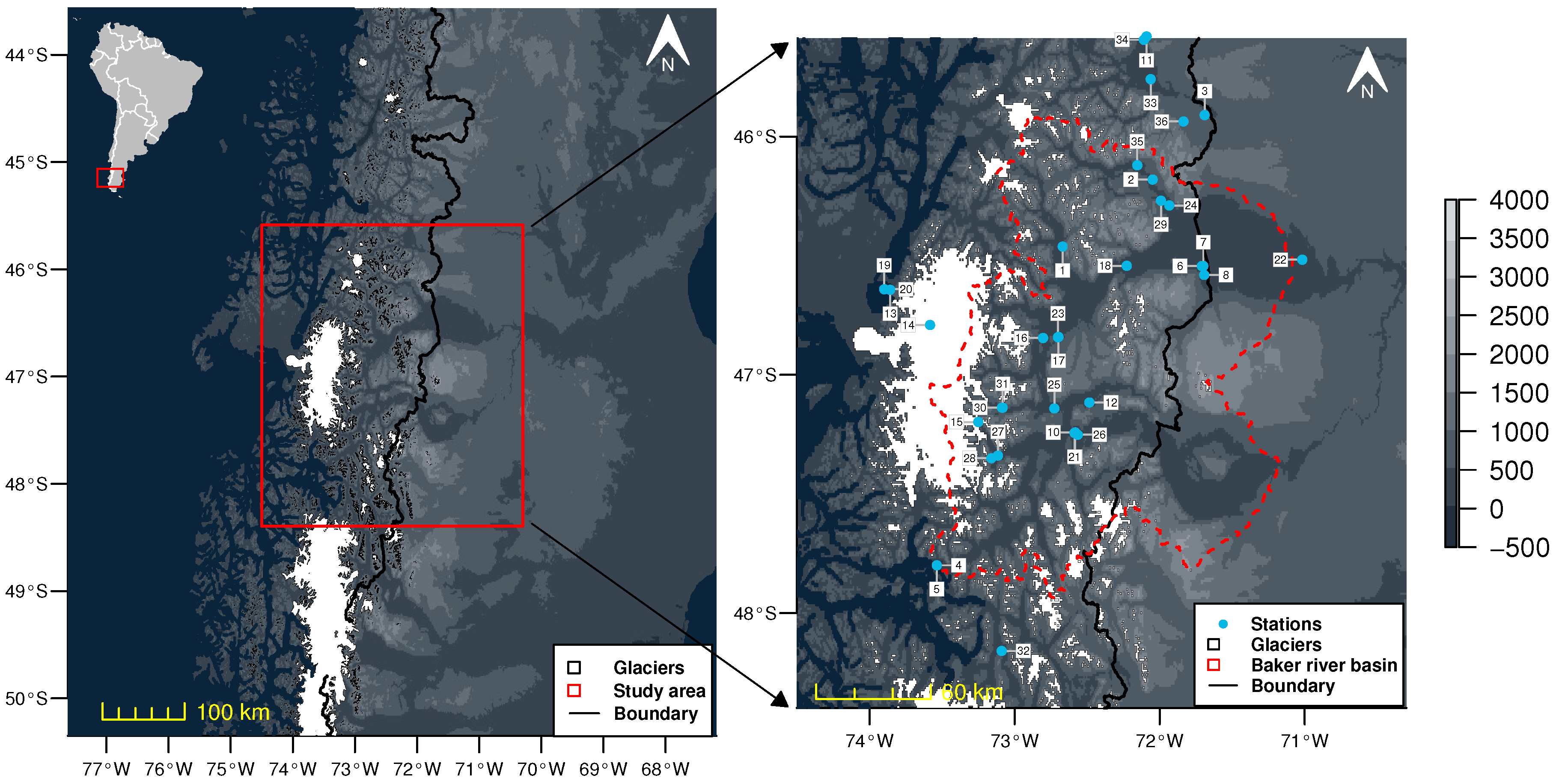
The region of interest corresponds to the Baker River basin, and the Northern Patagonia Ice Cap (NPI) (Figure 1) located in the Western (Chilean) Patagonia. In this region, the austral Andes perturbs the barometric waves that result in one of the most dramatic precipitation gradients on earth [14]. In western Patagonia, precipitation decreases abruptly to the east. The western side has a hyper humid climate with large precipitation at a synoptic scale that is magnified by the orographic effect. Frontal systems moving from the west are forced upward immediately after they cross over land, releasing most of the water content, and little moisture is left for the east side of Patagonia [15]. Precipitation is uniformly distributed around the year [16] with an increase during the winter months (see Aysen and Balmaceda stations, Figure 2 in [17]). This enables the formation of dense forests, large rivers, and glaciers, such as the NPI [14]. Zonal winds, on the other hand, influence seasonal air temperatures with a difference in mean temperature between summer and winter of 5 C at the ice caps to 15 C on the east side of west Patagonia [14]. The Baker River basin has an area of approximately 27,000 km; this basin produces the largest streamflow in Chile (>1000 m·s) with significant contributions from glacier melting from the east side of the NPI. The Baker River Basin is one of the most diverse systems and data-sparse regions in the world, with precipitation ranging from 220 to 1707 mm per year and elevations changes of more than 3000 m in less than 60 km of distance [1]. Storage from glaciers and lakes regulate streamflow in most of the rivers in the Baker Basin [1,18,19].
2.2. Meteorological Observations
We were able to access data for 36 weather stations in the area of study (Table 1) maintained by public institutions in Chile: Dirección General de Aguas (DGA) and glaciology (GDGA), Instituto de Investigaciones Agropecuarias (INIA), Dirección Metereológica de Chile (DMC), Centro de Datos Oceanográficos y Meteorológicos (CDOM), and Global Historical Climatology Network (GHCN). The parameters available are relative humidity (nine stations), precipitation (27 stations), pressure (six stations), wind speed (eight stations), daily mean air temperature (22 stations), and daily max and min air temperature (23 stations). From all the stations, we used 30 stations. We identify with yes the stations that we used and no the ones we did not use. They are stations measuring the same meteorological variables in a location but are maintained by different institutions, so we just kept one of them (i.e., Precipitation in Chile Chico see Table 1). Additionally, there are cases in which none of the configurations could obtain a result (i.e., Precipitation in Glaciar San Rafael), so, following [11], we ignored them to compare configuration performance. For that, we kept the stations with the Nash Sutcliffe Efficiency (NSE) score of above 0. More details are provided in the discussion section.
2.3. Climate Reanalysis Downscaling
Global datasets that are available for this region have resolutions that are not suitable for high-resolution studies and cannot capture processes that occur in small scales [19]. We will use the Weather Research Forecast (WRF) V4 [23] model to dynamically downscaled reanalysis data for the Baker River Basin and NPI. WRF is a NWP and atmospheric system designed for both research and operational applications [23]. WRF is used in operational forecasts in at least ten countries and hundreds of institutions for research purposes. In our study, we will use three different boundary conditions. First, ERA-interim atmospheric reanalysis, which is a dataset that goes from 1979 to 2018, the resolution is approximately 80 km with six hours of temporal resolution [24]. ERA5 is the latest reanalysis produced by the European Center for Medium-range Weather Forecast (ECMWF). ERA5 is an hourly product that ranges with a 0.25 × 0.25 degrees resolution [25,26]. And FNL0832 Operational Model Global Tropospheric Analyses (ds083.2) that goes every 6-hours from 1999-07-30 to present [27]. The calibration of NWP is impractical due to the thousands of parameters that would need to be adjusted. Therefore, the attention will be put on the physics options that the namelist provides. We follow a similar approach than [28,29,30].
For the model, we used two nested grids at 22.5 and 4.5 km (1:5 ratio) with 34 vertical levels (Figure 1). For the physics, we combined the options from [11,13]. Ruiz et al. [13] determined that for the convective parameterization the BMJ model (cu physics 2 in the namelist) produces better results, so we used it for the coarser domain at 22.5 km.
We used two micro-physics options, the simpler implementation WSM3 [31] and the Thompson implementation [32]. For the radiation, we used two combinations of physics to represent longwave and short wave radiation. The first pair spectral-band longwave and shortwave schemes used in the NCAR Community Atmosphere Model (CAM 3.0) for climate simulations [33]. The second pair is the Rapid Radiative Transfer Model (RRTM) Longwave [34] and the Dudhia [35] scheme, which has a simple downward integration of solar flux, accounting for tunable clear-air scattering, as well as water vapor absorption, and cloud albedo and absorption [23].
We used three Planetary Boundary Layer (PBL), the Yonsei University (YSU), which is the state of the art PBL for Medium-Range Forecast models. The Mellor-Yamada-Janjic (MYJ) PBL, a local implementation of the Mellor–Yamada 2.5 scheme [23]. Additionally, the Quasi-Normal Scale Elimination (QNSE) scheme with EDMF [36]. For the Land Surface Model (LSM), we used five-layer thermal diffusion with soil temperature only scheme and the Noah-MP (multi-physics) Land Surface Model [37,38]. We generated 24 combinations with these options using the main namelist’s options described below.
2.4. WRF Variables
The extraction of the data from WRF is straightforward. We used the WRF output variables PSFC [Pa] (surface pressure), T2 [K] (surface temperature), U10 and V10 [m s] (surface wind speed), RAIN+RAINNC [mm] (accumulated total precipitation), for relative humidity using Clausius–Clapeyron [39] (Equation (1)), we also need Q2 [kg kg] (mass mixing ratio).
where:
- T = temperature [K]
- p = pressure [Pa]
- q = specific humidity or the mass mixing ratio of water vapor to total air (dimensionless)
- = reference temperature (typically 273.16 K) [K]
2.5. Evaluation
In the evaluation process, we compared the model results with the meteorological observations (Table 1). There are multiple indicators to evaluate the quality of the results, depending on the application [40]. In this work, we use: Nash Sutcliffe Efficiency (NSE) (Equation (2)), correlation (Equation (3)), and percentage bias (PBIAS) (Equation (4)) that measure the average tendency of the simulated data. The ratio of the root means square error to the standard deviation of measured data (RSR) (Equation (5)) that standardizes Root Medium Square Error (RMSE) using the observations standard deviation (STDEV).
Additionally, we used a more recent indicator, the Kling-–Gupta efficiency (KGE) [41] (Equation (6)), that seeks to reduce the errors of NSE by decreasing the distance of the three-component of NSE (correlation, mean squared error, and variability) [41]. KGE is often used for calibration.
where:
and
where: r = correlation coefficient, = mean value of simulation/observation, = standard deviation of simulation/observation.
2.6. Selection of the Best Configuration
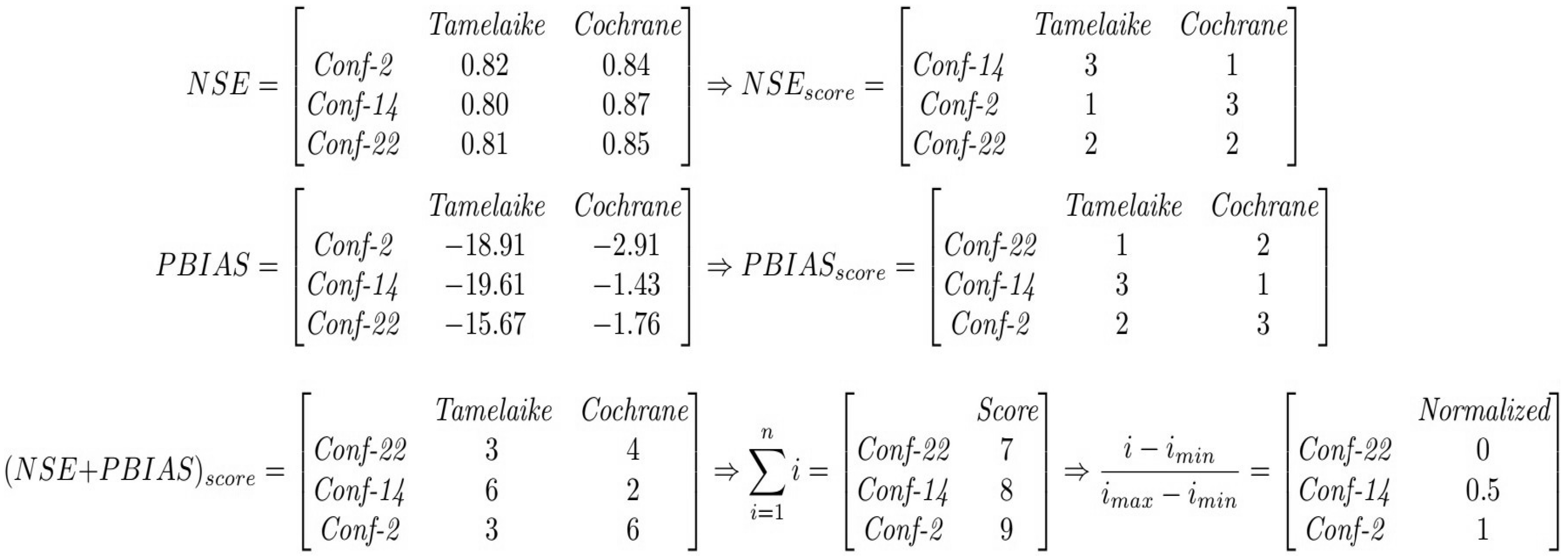
We identified the best configuration through a scoring procedure [42]. For this, in a station, we select a variable (i.e., precipitation) and a statistic (i.e., NSE), we sorted the performance of the configuration from better to worse (Figure 2, NSE). A value of 1 is assigned to the best-performing configuration and add a unit to the next. This process is repeated for each statistic in all of the stations (i.e., Figure 2, PBIAS). Subsequently, the scores obtained for each configuration are added (Figure 2, NSE+PBIAS). The configuration with the lower value is the one that performs better for the variable. Then we normalized the scores so we can compare variables with a different number of observations points. In Figure 2, we provided an example with three configurations and two stations for mean temperature. In the example provided in Figure 2, the best configuration is Conf-22 and the worse is Conf-2.
3. Results
3.1. Configuration Performance
Table 4 shows the ranking for the performance of the 24 WRF configurations used in this work. The best five settings for precipitation were 9, 10, 13, 11, and 1. For relative humidity, the best were 2, 13, 14, 9, and 1. For mean temperature, the best performance was obtained with 14, 2, 22, 10, and 19. For maximum temperature, 14, 20, 22, 2, and 10 perform better. For the minimum temperature, the best settings were 2, 10, 6, 7, and 22. Finally, when considering all of the variables, the best parameterizations were 10, 14, 2, 9, and 22.
3.2. Spatial Distribution of the Result
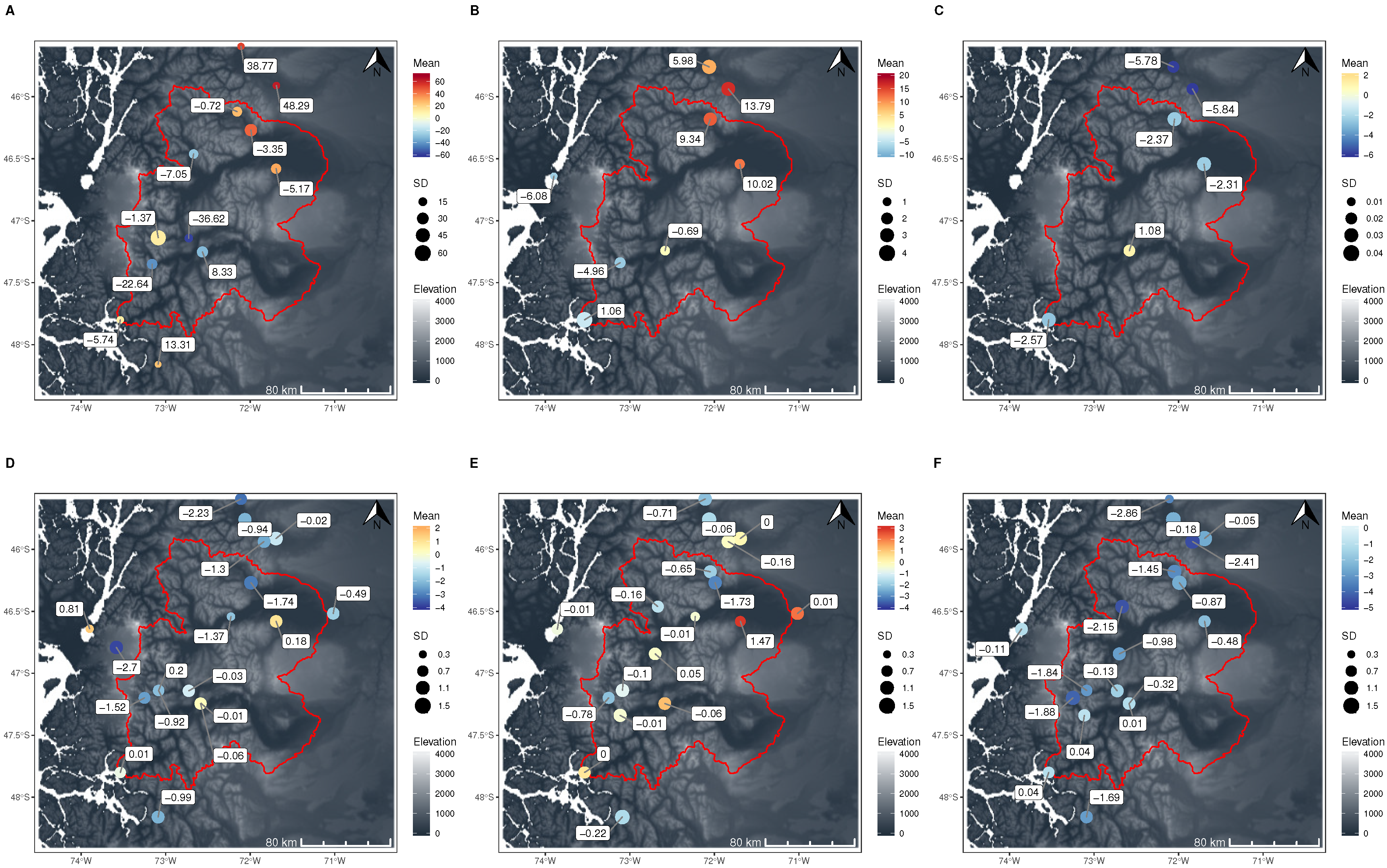
Figure 3 shows the spatial distribution of the percentage bias for precipitation, relative humidity, and surface pressure, and bias for mean, minimum, and maximum temperatures for the best five configurations according to Table 4. From all of the variables evaluated in this work, precipitation was the variable with more bias among configurations and spatial distribution. The temperature, on the other hand, was the variable with better results.
3.2.1. Precipitation
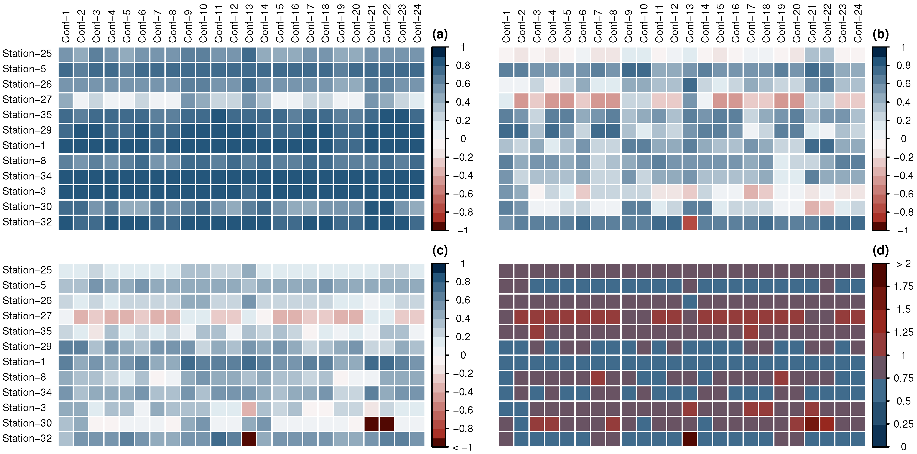
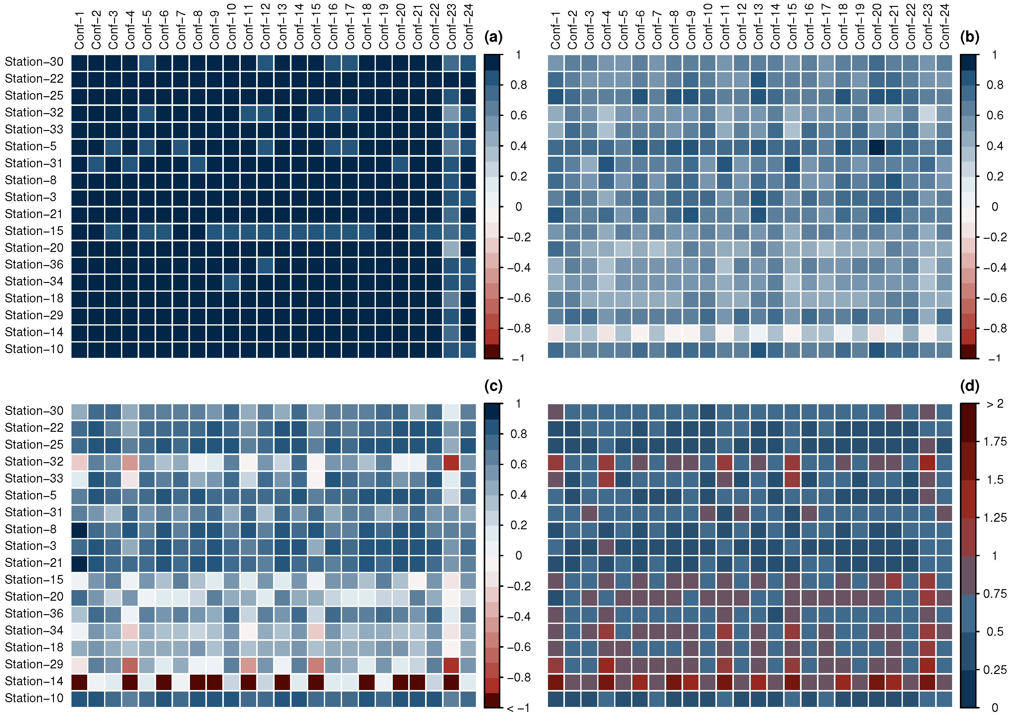
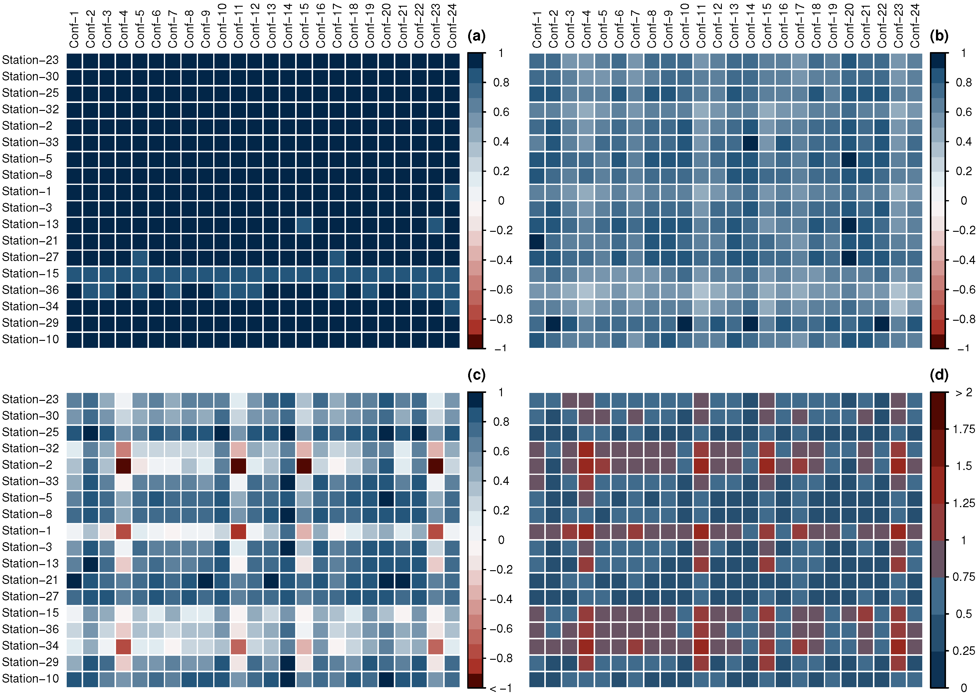
Most of the configurations, on average, can do a decent or good job with average correlations above 0.66 and RSRs lower than 0.88. However, they do not have a homogenous performance for the entire domain. Correlation for conf-5, 7, and 8, for example, range from 0 to 0.85. Conf-9 and 10 that use the same parameterization except for the land surface model have the best performance on average. Conf-9 and 10 have a mean correlation of 0.75, with a minimum of 0.53 and 0.43, respectively. Additionally, Conf- 9 and 10 are the only stations that have NSE above 0.05 for all of the stations with an average of 0.43 (Figure 3A and Figure 4).
3.2.2. Temperature
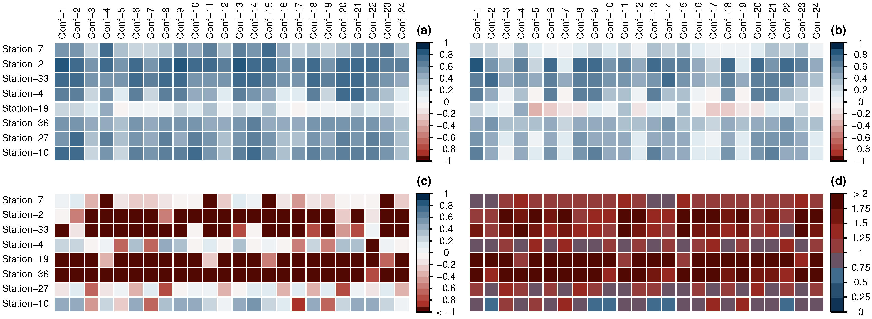
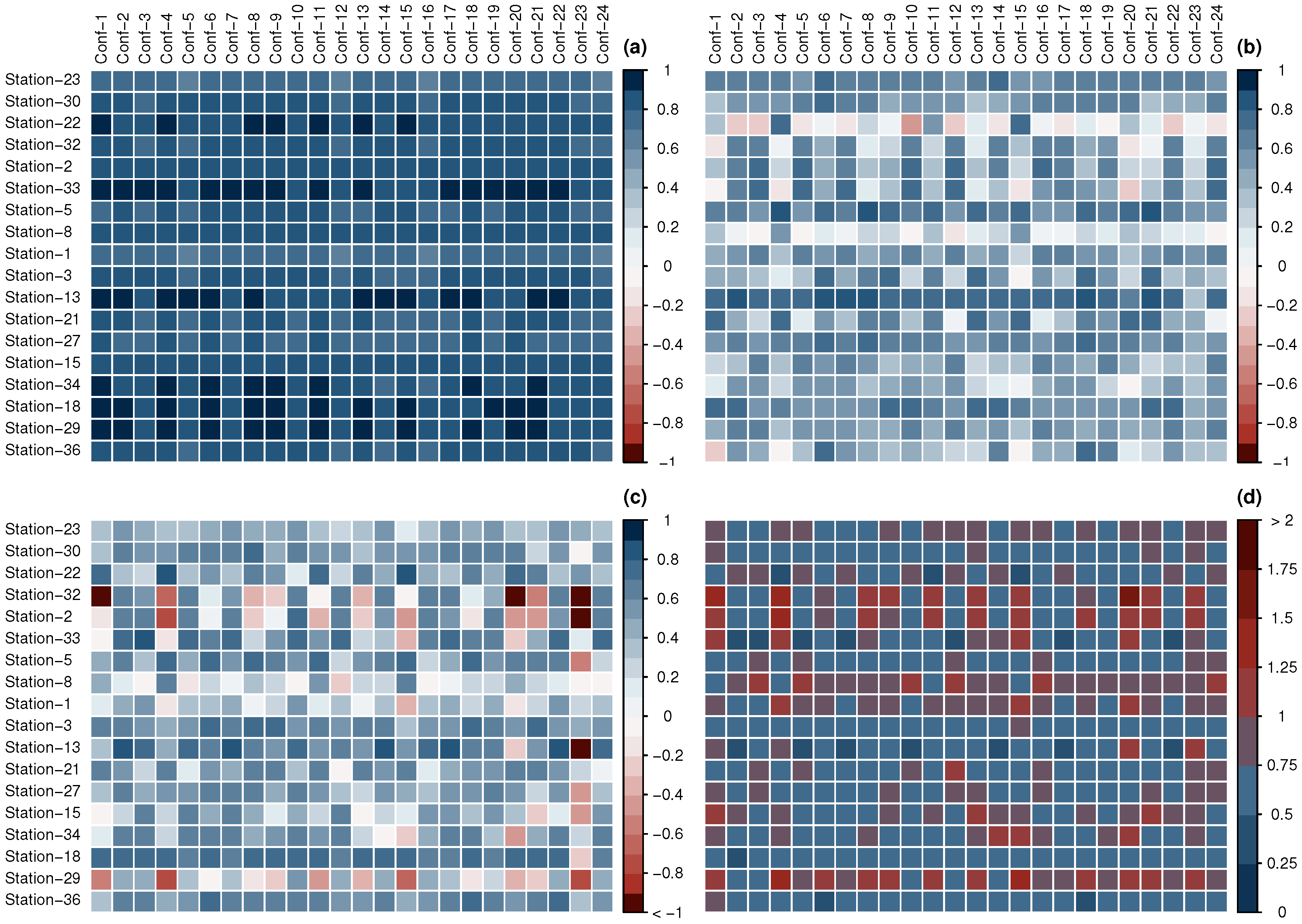
Temperature in its three versions: mean (Figure 5), maximum (Figure A1) and minimum (Figure A2), has better results than the other variables. All of the models have a correlation above 0.87 for all the stations with an average maximum bias of 2.7 degrees Celsius. As a consequence, NSE and KGE, in general, are above 0.5 and RSR lower than 1. All of the estimation results are excellent, except for HNG San Rafael on the west side of NPI, where they are not great but acceptable, which may be a consequence of the extreme conditions on the ice cap.
3.2.3. Relative Humidity and Surface Pressure
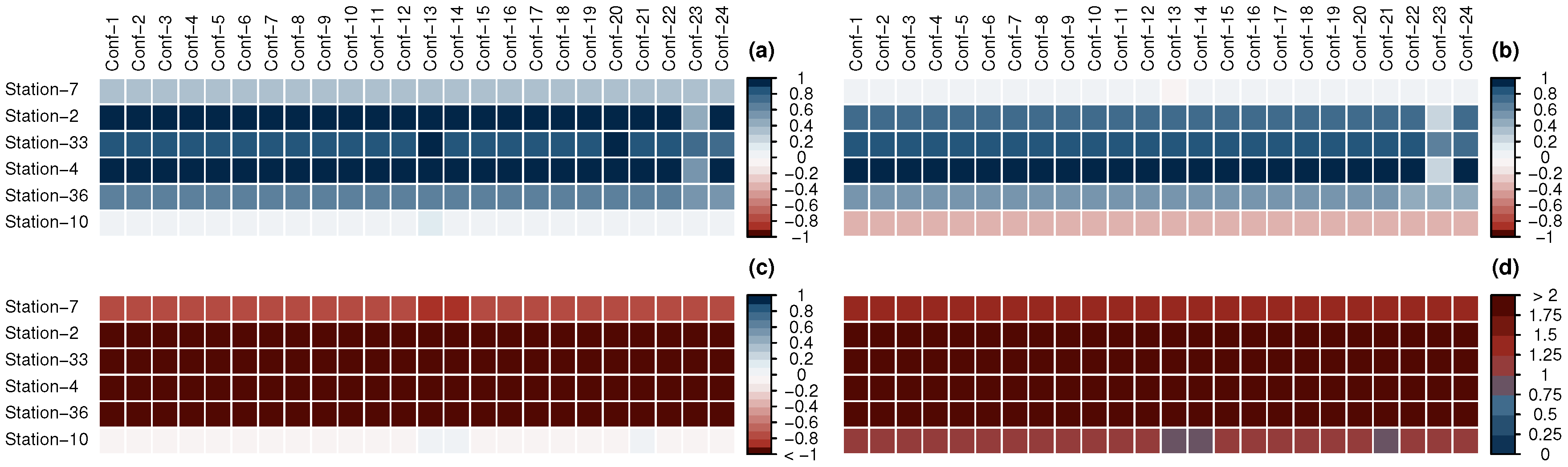
In general, the results for relative humidity have problems with RSR that affect NSE scores (Figure 6). All of the configurations have mean RSR above 1, which indicated a large bias in the data. As a result, none of the configurations have average NSE above 0. Therefore, if we use NSE, all of the results for relative humidity are inadequate. The same is found in surface pressure (Figure A3), where the model for all configurations does a very poor job with RSR and, consequently, NSE. On the other hand, percentage bias results are good (lower than 15%), and correlations are acceptable (above 0.5 for most of the stations), which ends up in acceptable KGEs, above 0.42, for 15 out 24 configurations. Therefore, the errors may be related to the poor performance of the surface pressure calculation more than the mixing ratio, given that the relative humidity calculation depends on the results of surface pressure (Equation (1)). Therefore, the performance of the models for relative humidity and surface pressure, in particular, the ones with better scores in Table 4, is not good, although that is not conclusive. It depends on which statistic is considered to evaluate the results.
3.2.4. Wind Speed
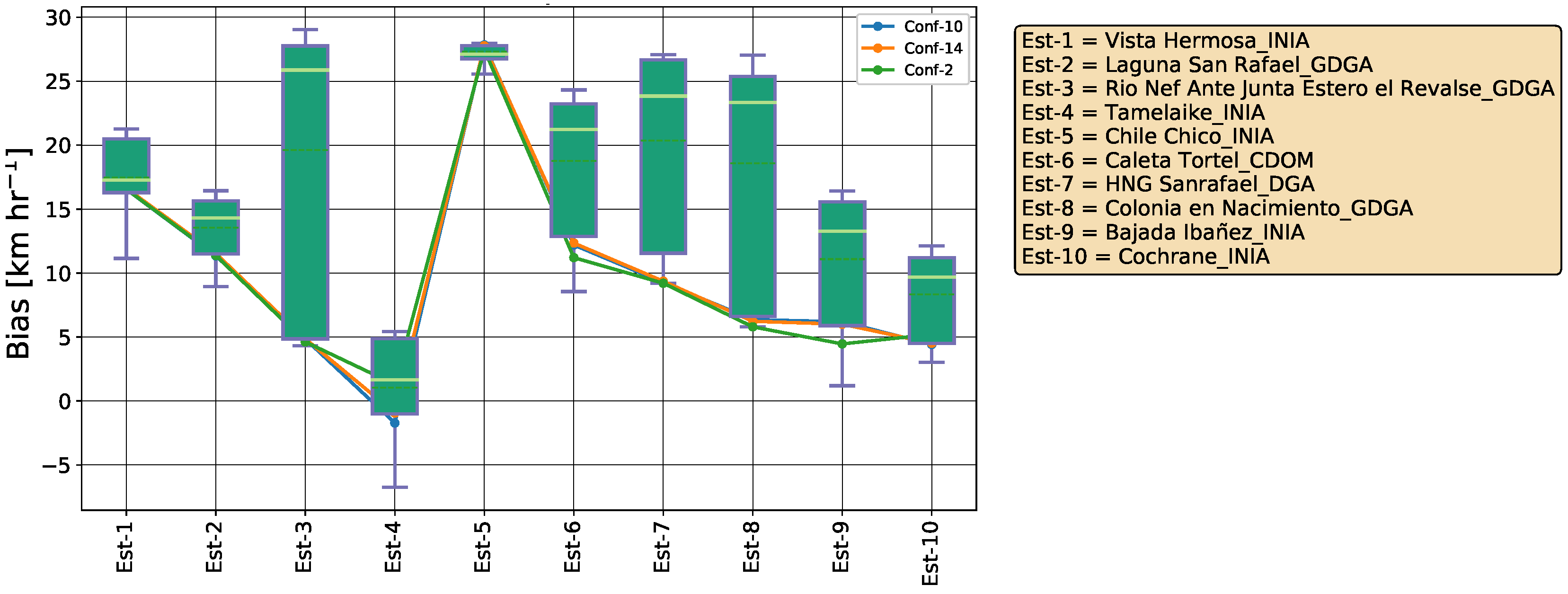
From all of the variables, wind speed has the worst results. In all of the stations, it performs poorly in daily correlation and bias; therefore, all the other statistics are weak. In Figure 7, we can see the bias for ten stations wherein most of them the bias is very high. The reason why the wind speed’s results are not good is probably because of a poor representation of the topography that can affect the wind speed at scales of meters in particular in mountain areas. The model has a resolution of 4.5 km, which makes it impossible to capture local features. A secondary source of error maybe the fact that the stations that measure wind speed are not always at 10 m following the WMO standard [43]. In Figure 7, we show the performance of all the configurations in a box plot for ten stations. We also include lines for the three best configurations (lower bias) in wind speed that have acceptable results [44] in the stations around the Baker River (stations 3, 4, 8, 9, 10).
3.3. Multiple Forcing
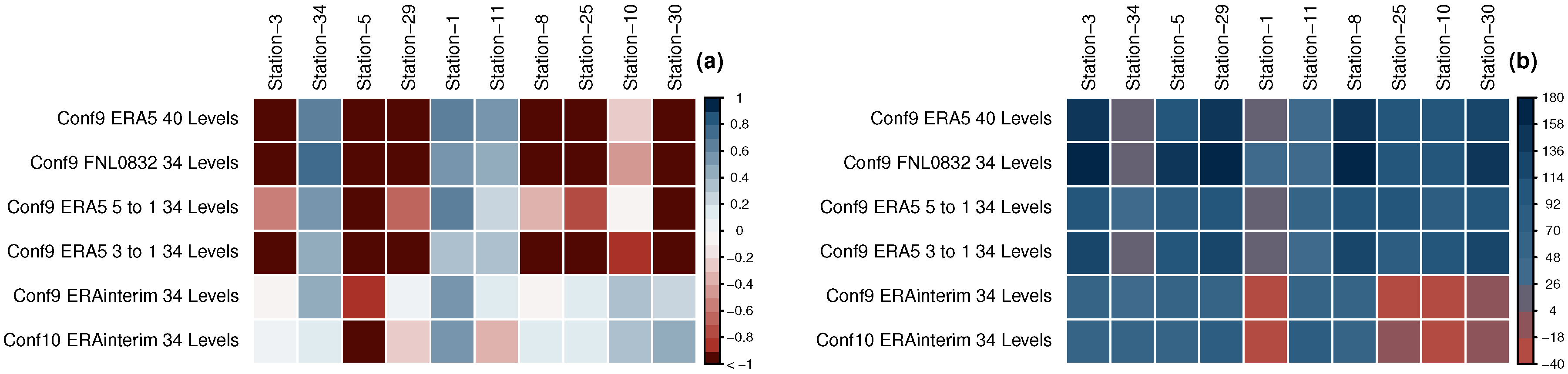
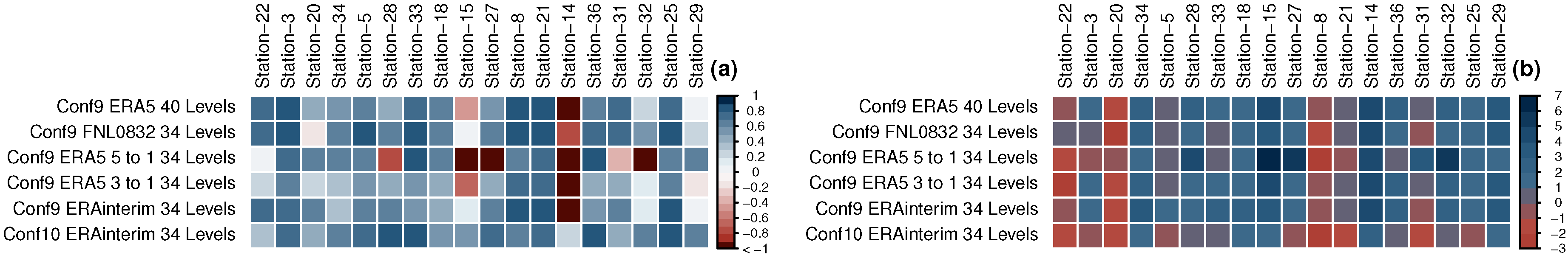
Configuration 9 gives the best results for precipitation (Table 4). We used configuration 9 with two other datasets (Era5 and FNL0832) in 2017 to compare different forcing performances. Additionally, we changed the number of vertical levels from 34 to 40 in one of the models with ERA5. Then considering that ERA5 has better resolution, we added another simulation in which we maintain the finer resolution at 4.5 km and the outer domain as a resolution of 13.5 km; therefore, the ratio between the nested domains is 3 to 1. For the precipitation, the model that used ERA-interim performs better than ERA5 and FNL0832; the average NSE is higher than 0.2, while all the other forcing have average NSE lower than 0. The percentage bias is lower than 40%, while the other forcings have a percentage bias above 76% (Figure 8). On the other hand, for average temperature, the model that used FNL0832 forcing, outperformed all ERA-interim and ERA5 reanalysis. The average bias is 1.5 C and NSE 0.55. However, configuration 10 that was run with ERA-interim, which is the best configuration according to Table 4, provides better results with an average absolute bias of 1.18 C and an NSE of 0.63 (Figure 9).
4. Discussion
4.1. Observation Network Quality
There are almost 40 official weather stations in the study area. Given the latitude and difficulties, it seems that the region is well instrumented. However, we found several limitations and deficiencies with the observation network. The first limitation we faced is related to discontinuities. The datasets are generally incomplete, with several windows with no data, which makes it harder to rely on all of the stations. The discontinuities may be generated, because it is difficult and expensive to maintain instruments in Patagonia; access is difficult, and the government’s presence is unfrequent. This situation had improved in the last decade, particularly after 2017, when several stations started to operate. Even other meteorological variables are being observed now, such as solar radiation (not used here) and relative humidity.
There is duplication in the observations. Different institutions are observing the same variables almost in the same place. In Table 1, we can see that there are several places where DGA, INIA, DCM are measuring the same meteorological variables. For example, in Chile Chico, there are three stations measuring precipitation, minimum and maximum temperature. The same situation is found in Cochrane. This shows a lack of coordination among public institutions. If there was better communication, the repeated weather stations could be moved to other areas to increase the points with observations.
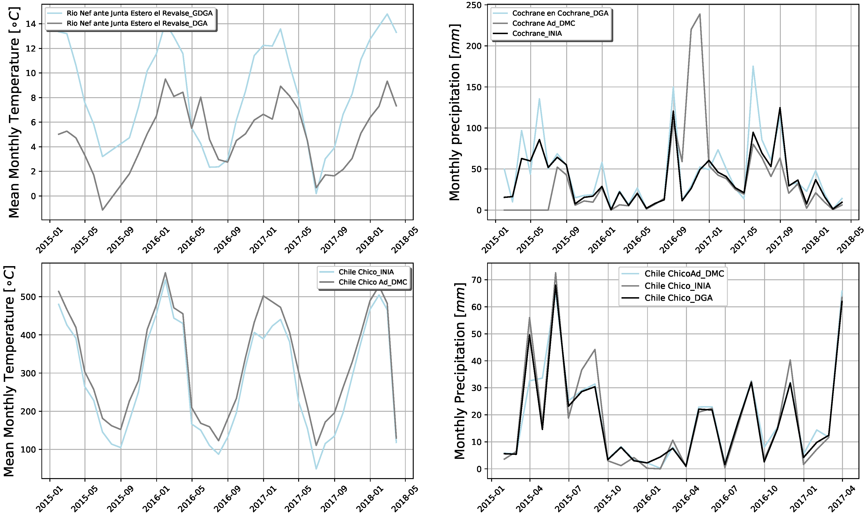
The quality of the observations is not guaranteed. Dussaillant J. et al. [1] mentioned that, in this region, data quality is a limitation. This assertion is corroborated in Figure 10, where we compared observations in the same location from different institutions, and we can see that the values not always matched. We also compared observations from the same institution but published in two different places (DGA, GDGA). DGA provided the data aggregated daily, GDGA provided the data hourly. However, when we aggregated the values from GDGA, they did not match with the data from DGA (Figure 10, top left panel). Then, we also have the situation, where data collected for different institutions in the same location do not match up (Figure 10).
4.2. Model Selection
Microphysics selection affects the non-convective precipitation at grid scales [45]. The complexity of the microphysics increases as the resolution reaches convection-permitting levels where microphysics with graupel size representation in the scheme is essential to the precipitation production [46]. The PBL plays a critical role in the transportation of energy (including momentum, heat, and moisture) into the upper layers of the atmosphere. It acts as a feedback mechanism in wind circulation [47]. PBL parameterization schemes are essential for the better simulations of wind components and turbulence in the lower part of the atmosphere [48]. LSMs usually compute heat and moisture fluxes over land and sea-ice points and provide them to the considered PBL schemes [49], which may affect the performance of WRF [50]. The radiation scheme seeks to estimate total radiative flux [51].
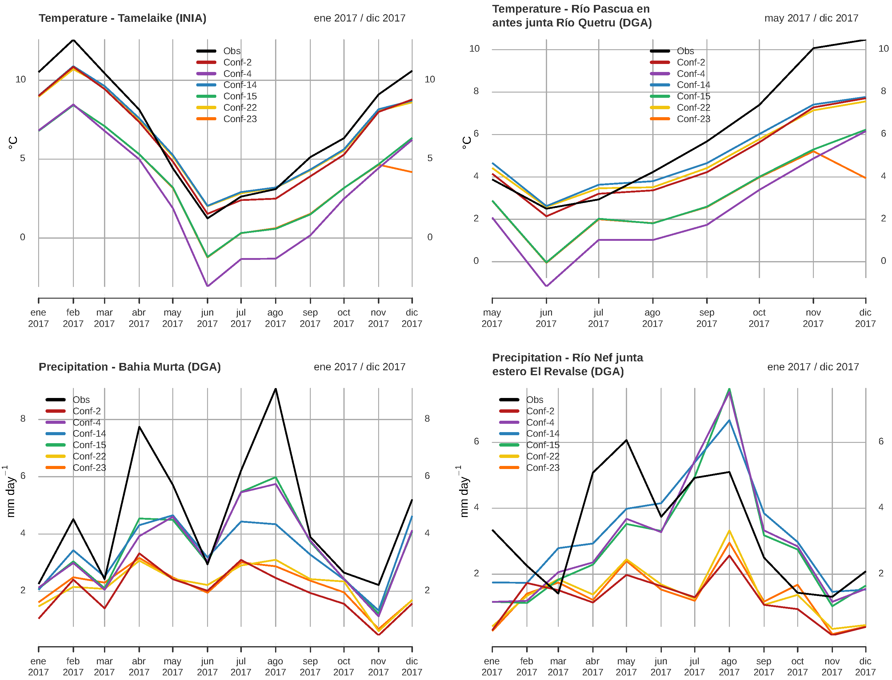
The best five combinations of physics for precipitation have in common that four out of five used RRTM for longwave radiation, Dudhia for short wave radiation, YSU for PBL, and NoahMP for the land surface model. The top three used Thompson for microphysics, and none of them use QNSE for PBL. For mean temperature, four out of the five best configurations use YSU for PBL, and five out of five used the five-Layer Thermal for the LSM. For the other options, WSM3 performs better than Thompson for the microphysics, and for the long and short radiation, CAM models rank better. For the maximum and minimum temperature, the models’ performance is similar to mean temperature, except that only three out of five configurations used YSU for PBL, and two used QNSE. And four out of the five best configurations used the 5-Layer Thermal for the LSM. Finally, for RH, all the best five configurations used YSU for PBL, four out of the five used WSM3 for microphysics, and three out of five used RRTM for longwave, and Dudhia for short wave radiation. In Figure 11, we provide examples of different configuration in particular stations that have large differences in performance.
4.3. Multiple Forcing and General Remarks
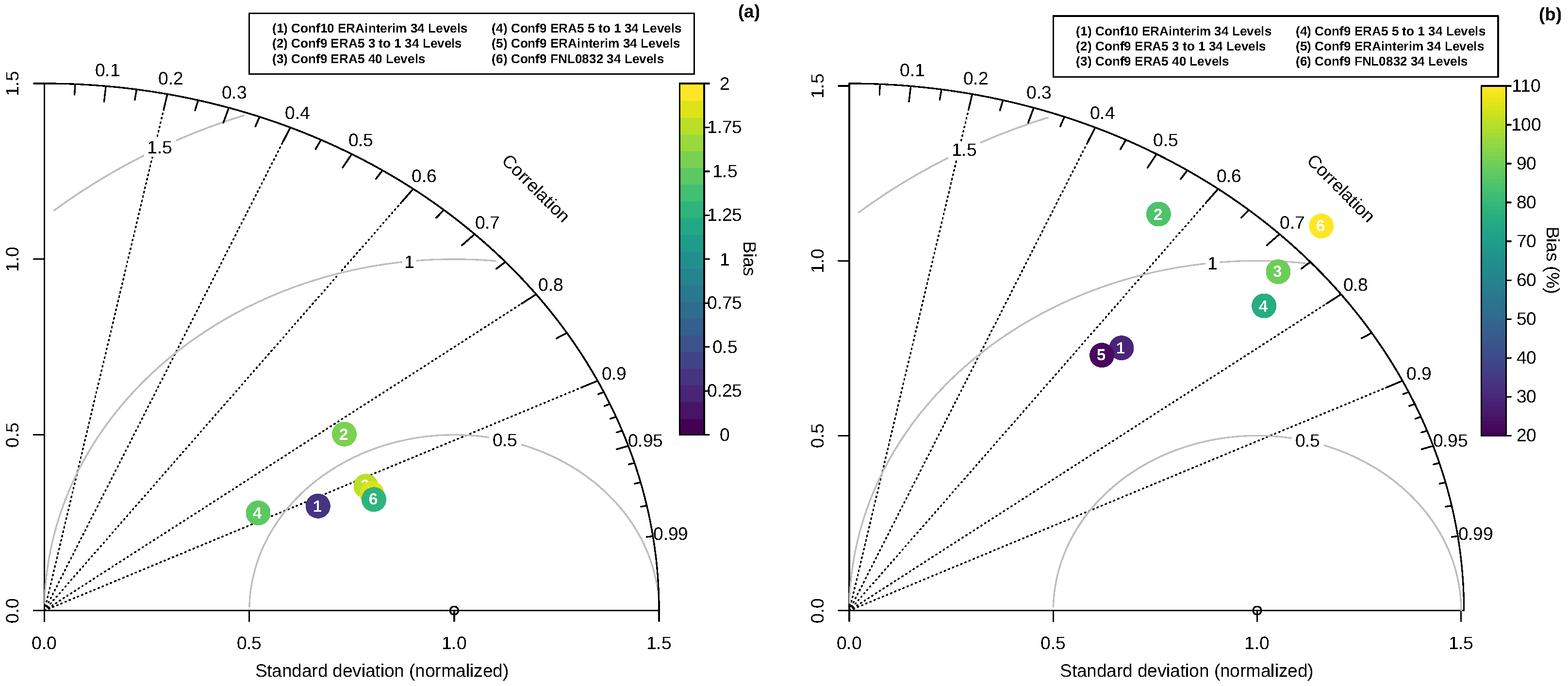
In our experiment, Era-interim provided a better result, by a long-distance, than ERA-5 and FNL0832 for precipitation. ERA 5 has similar results in average for the root mean square than ERA-Interim, as it can be seen in the Taylor diagram (Figure 12) for temperature and precipitation. It also has a better mean correlation. However, for precipitation, the mean for the standard deviation for ERA5 is very high when compared to ERA-Interim, which explains that it ended up with a more inferior score in our selection procedure.
FNL0832 gave better results in the case of temperature; however, the performance of all the models was good. Therefore, working with ERA-Interim from 1978 to 2018 seems to be the best option in this region. We did not experiment with changes in resolution, which may have improved results with ERA-5 that has better spatial and temporal resolution.
In general, the model did well for temperature (mean, minimum and maximum) for most of the stations. Precipitation was good, but just a few configurations stood out (conf-9 and conf-10). Surface pressure was not good or bad; the results were okay if we used KGE, but they were not okay if we used NSE. There is a systematic low RSR for all the stations and configurations. We think that there may be a couple of reasons why this happens. The first is the resolution, which is 4.5 km, so the details of the terrain are smoothed, and the second is that the model surface level may not be well represented, so it needs to be evaluated in more detail. The errors for relative humidity are similar to the errors in surface pressure. Large errors in RH were also found by [49] in India. However, Cohen et al. [48] obtained good results for specific humidity using YSU and MYJ for the PBL in the southeastern U.S. Therefore, we think that the pressure is the primary source of error since we used it along to calculate RH (Equation (1)). And Finally, none of the models could capture wind speed; in general, the bias was high. This could be because the model provides wind velocity at 10 m from the ground. The stations are not higher than 2–4 m in general, or because the terrain representation and station location are not well represented. Therefore, this is something that needs to be explored in more detail.
In summary, from more to less certain. We found that for PBL, the best option is to use YSU, which also gives good results in central Southamerica by [13,47], Korea [48] and Antarctic [52]. For the LSM, the best option is the 5-Layer Thermal. WRF is sensitive to the selection of LSM [49,50]. In Ethiopia, Teklay et al. [50] found that the five-Layer Thermal model had a low cold bias for maximum and minimum temperature. However, for precipitation, Noah has better results, which is similar to our results. RRTM performs well for longwave; it also performs well in the Antarctic Winter [52]. Dudhia does better than CAM for short wave radiation. Zempila et al. [53] found that Dudhia provides better results than more sophisticated schemes in a study in Greece, particularly for clear skies. For the microphysics, Thompson does better work. However, Jeworrek et al. [46] indicates that the microphysics does not have a significant impact when working at the spatial resolution of this study. For the LSM, we did not explore the multiple options that the NoahMP model provides and used the default settings, so there may be NoahMP configurations that can do better, so we left that open for future research. For the PBL in general, QNSE is the one that had the lower performance. Summarizing, the best set of physics in our numerical experiment is YSU for PBL, for the LSM, five-Layer Thermal for the LSM, RRTM for longwave, Dudhia for short wave radiation, and Thompson for the microphysics.
Author Contributions
Conceptualization, M.S.-V.; methodology, M.S.-V; validation, M.S.-V.; formal analysis, M.S.-V. and F.M.-C; writing–original draft preparation, M.S.-V. and F.M.-C. All authors have read and agreed to the published version of the manuscript.
Funding
This research was funded by the Agencia Nacional de Investigacion y Desarrollo (ANID) Chile Fondecyt Iniciacion N 11170609.
Conflicts of Interest
The authors declare no conflict of interest.
Appendix A. Comparison Result for Maximum and Minimum Temperature, and Surface Pressures
Appendix A.1. Maximum and Minimum Temperature Results
Figure A1.
Matrix of statistics for maximum temperature: (a) correlation, (b) KGE, (c) NSE, (d) RSR.
Figure A1.
Matrix of statistics for maximum temperature: (a) correlation, (b) KGE, (c) NSE, (d) RSR.

Figure A2.
Matrix of statistics for minimum temperature: (a) correlation, (b) KGE, (c) NSE, (d) RSR.
Figure A2.
Matrix of statistics for minimum temperature: (a) correlation, (b) KGE, (c) NSE, (d) RSR.

Appendix A.2. Surface Pressure Results
Figure A3.
Matrix of statistics for surface pressure: (a) correlation, (b) KGE, (c) NSE, (d) RSR.

References
- Dussaillant, J.A.; Buytaert, W.; Meier, C.; Espinoza, F. Hydrological regime of remote catchments with extreme gradients under accelerated change: The Baker basin in Patagonia. Hydrol. Sci. J. 2012, 57, 1530–1542. [Google Scholar] [CrossRef]
- Fosser, G.; Khodayar, S.; Berg, P. Benefit of convection permitting climate model simulations in the representation of convective precipitation. Clim. Dyn. 2014, 44, 45–60. [Google Scholar] [CrossRef] [Green Version]
- Pal, S.; Chang, H.I.; Castro, C.L.; Dominguez, F. Credibility of convection-permitting modeling to improve seasonal precipitation forecasting in the southwestern United States. Front. Earth Sci. 2019, 7, 1–15. [Google Scholar] [CrossRef] [Green Version]
- Maurer, E.P.; Wood, A.W.; Adam, J.C.; Lettenmaier, D.P.; Nijssen, B. A Long-Term Hydrologically Based Dataset of Land Surface Fluxes and States for the Conterminous United States*. J. Clim. 2002, 15, 3237–3251. [Google Scholar] [CrossRef] [Green Version]
- Mearns, L.; Bukovsky, M.; Pryor, S.; Magana, V. Climate Change in North America; Regional Climate Studies; Springer International Publishing: Cham, Switzerland, 2014; pp. 201–250. ISBN 978-3-319-03768-4. [Google Scholar]
- Schaefer, M.; Machguth, H.; Falvey, M.; Casassa, G. Modeling past and future surface mass balance of the Northern Patagonia Icefield. J. Geophys. Res. Earth Surf. 2013, 118, 571–588. [Google Scholar] [CrossRef] [Green Version]
- Mearns, L.O.; Sain, S.; Leung, L.R.; Bukovsky, M.S.; McGinnis, S.; Biner, S.; Caya, D.; Arritt, R.W.; Gutowski, W.; Takle, E.; et al. Climate change projections of the North American Regional Climate Change Assessment Program (NARCCAP). Clim. Chang. 2013, 120, 965–975. [Google Scholar] [CrossRef] [Green Version]
- Mearns, L.O.; Gutowski, W.; Jones, R.; Leung, R.; McGinnis, S.; Nunes, A.; Qian, Y. A Regional Climate Change Assessment Program for North America. Eos Trans. Am. Geophys. Union 2009, 90, 311. [Google Scholar] [CrossRef]
- Mearns, L.O.; Gutowski, W.J.; Jones, R.; Leung, L.Y.; McGinnis, S.; Nunes, A.M.B.; Qian, Y. The North American Regional Climate Change Assessment Program Dataset; National Center for Atmospheric Research Earth System Grid Data Portal: Boulder, CO, USA, 2007; Available online: http://www.earthsystemgrid (accessed on 3 May 2016).
- Müller, O.V.; Lovino, M.A.; Berbery, E.H. Evaluation of WRF Model Forecasts and Their Use for Hydroclimate Monitoring over Southern South America. Weather Forecast. 2016, 31, 1001–1017. [Google Scholar] [CrossRef] [Green Version]
- Villarroel, C.; Carrasco, J.F.; Casassa, G.; Falvey, M. Modeling Near-Surface Air Temperature and Precipitation Using WRF with 5-km Resolution in the Northern Patagonia Icefield: A Pilot Simulation. Int. J. Geosci. 2013, 4, 1193–1199. [Google Scholar] [CrossRef] [Green Version]
- Yáñez-Morroni, G.; Gironás, J.; Caneo, M.; Delgado, R.; Garreaud, R. Using the Weather Research and Forecasting (WRF) model for precipitation forecasting in an Andean region with complex topography. Atmosphere 2018, 9, 304. [Google Scholar] [CrossRef] [Green Version]
- Ruiz, J.J.; Saulo, C.; Nogués-Paegle, J. WRF Model Sensitivity to Choice of Parameterization over South America: Validation against Surface Variables. Mon. Weather Rev. 2010, 138, 3342–3355. [Google Scholar] [CrossRef]
- Garreaud, R.; Lopez, P.; Minvielle, M.; Rojas, M. Large-scale control on the Patagonian climate. J. Clim. 2013, 26, 215–230. [Google Scholar] [CrossRef]
- Garreaud, R.D. The Andes climate and weather. Adv. Geosci. 2009, 22, 3–11. [Google Scholar] [CrossRef] [Green Version]
- Masiokas, M.H.; Rabatel, A.; Rivera, A.; Ruiz, L.; Pitte, P.; Ceballos, J.L.; Barcaza, G.; Soruco, A.; Bown, F.; Berthier, E.; et al. A Review of the Current State and Recent Changes of the Andean Cryosphere. Front. Earth Sci. 2020, 8, 1–27. [Google Scholar] [CrossRef]
- Aravena, J.C.; Luckman, B.H. Spatio-temporal rainfall patterns in Southern South America. Int. J. Climatol. 2009, 29, 2106–2120. [Google Scholar] [CrossRef]
- Bury, J.T.; Mark, B.G.; McKenzie, J.M.; French, A.; Baraer, M.; Huh, K.I.; Zapata Luyo, M.A.; Gómez López, R.J. Glacier recession and human vulnerability in the Yanamarey watershed of the Cordillera Blanca, Peru. Clim. Chang. 2010, 105, 179–206. [Google Scholar] [CrossRef] [Green Version]
- Krogh, S.A.; Pomeroy, J.W.; McPhee, J. Physically Based Mountain Hydrological Modeling Using Reanalysis Data in Patagonia. J. Hydrometeorol. 2015, 16, 172–193. [Google Scholar] [CrossRef] [Green Version]
- Farr, T.G.; Rosen, P.A.; Caro, E.; Crippen, R.; Duren, R.; Hensley, S.; Kobrick, M.; Paller, M.; Rodriguez, E.; Roth, L.; et al. The Shuttle Radar Topography Mission. Rev. Geophys. 2007, 45, RG2004. [Google Scholar] [CrossRef] [Green Version]
- Davies, B. GLIMS Glacier Database; The National Snow and Ice Data Center: Boulder, CO, USA, 2012; Available online: http://www.glims.org/maps/glims (accessed on 21 May 2020). [CrossRef]
- GLIMS and NSIDC. Global Land Ice Measurements from Space Glacier Database; The International GLIMS Community and The National Snow and Ice Data Center: Boulder CO, USA, 2005; updated 2020. [Google Scholar] [CrossRef]
- Skamarock, W.C.; Klemp, J.B.; Dudhia, J.; Gill, D.O.; Liu, Z.; Berner, J.; Wang, W.; Powers, J.G.; Duda, M.D.; Barker, D.M.; et al. A Description of the Advanced Research WRF Version 4. NCAR Tech. Note NCAR/TN-556+STR; Technical Report; NCAR: Boulder, CO, USA, 2019. [Google Scholar] [CrossRef]
- Dee, D.P.; Uppala, S.M.; Simmons, A.J.; Berrisford, P.; Poli, P.; Kobayashi, S.; Andrae, U.; Balmaseda, M.A.; Balsamo, G.; Bauer, P.; et al. The ERA-Interim reanalysis: Configuration and performance of the data assimilation system. Q. J. R. Meteorol. Soc. 2011, 137, 553–597. [Google Scholar] [CrossRef]
- Copernicus Climate Change Service (C3S). ERA5: Fifth Generation of ECMWF Atmospheric Reanalyses of the Global Climate. Copernicus Climate Change Service Climate Data Store (CDS). 2017. Available online: https://cds.climate.copernicus.eu/cdsapp#!/home (accessed on 4 November 2019).
- Hersbach, H.; Bell, B.; Berrisford, P.; Horányi, A.; Muñoz-Sabater, J.; Nicola, J.; Radu, R.; Schepers, D.; Simmons, A.; Soci, C.; et al. Global reanalysis: Goodbye ERA-Interim, hello ERA5. In Meteorology Section of ECMWF Newsletter No. 159; European Centre for Medium-Range Weather Forecasts: Reading, UK, 2019; pp. 17–24. [Google Scholar] [CrossRef]
- NCAR. NCEP FNL Operational Model Global Tropospheric Analyses, Continuing from July 1999; Research Data Archive at the National Center for Atmospheric Research, Computational and Information Systems Laboratory: Boulder, CO, USA, 2000. [Google Scholar] [CrossRef]
- Ikeda, K.; Rasmussen, R.; Liu, C.; Gochis, D.; Yates, D.; Chen, F.; Tewari, M.; Barlage, M.; Dudhia, J.; Miller, K.; et al. Simulation of seasonal snowfall over Colorado. Atmos. Res. 2010, 97, 462–477. [Google Scholar] [CrossRef]
- Rasmussen, R.; Liu, C.; Ikeda, K.; Gochis, D.; Yates, D.; Chen, F.; Tewari, M.; Barlage, M.; Dudhia, J.; Yu, W.; et al. High-resolution coupled climate runoff simulations of seasonal snowfall over Colorado: A process study of current and warmer climate. J. Clim. 2011, 24, 3015–3048. [Google Scholar] [CrossRef] [Green Version]
- Liu, C.; Ikeda, K.; Rasmussen, R.; Barlage, M.; Newman, A.J.; Prein, A.F.; Chen, F.; Chen, L.; Clark, M.; Dai, A.; et al. Continental-scale convection-permitting modeling of the current and future climate of North America. Clim. Dyn. 2016, 1–25. [Google Scholar] [CrossRef]
- Hong, S.Y.; Dudhia, J.; Chen, S.H. A revised approach to ice microphysical processes for the bulk parameterization of clouds and precipitation. Mon. Weather Rev. 2004, 132, 103–120. [Google Scholar] [CrossRef]
- Thompson, G.; Field, P.R.; Rasmussen, R.M.; Hall, W.D. Explicit forecasts of winter precipitation using an improved bulk microphysics scheme. Part II: Implementation of a new snow parameterization. Mon. Weather Rev. 2008, 136, 5095–5115. [Google Scholar] [CrossRef]
- Collins, W.D.; Rasch, P.J.; Boville, B.A.; Hack, J.J.; McCaa, J.R.; Williamson, D.L.; Kiehl, J.T.; Briegleb, B. Description of the NCAR Community Atmosphere Model (CAM 3.0), NCAR Technical Note, NCAR/TN-464+STR; Technical Report; NCAR: Boulder, CO, USA, 2004. [Google Scholar]
- Mlawer, E.J.; Taubman, S.J.; Brown, P.D.; Iacono, M.J.; Clough, S.A. Radiative transfer for inhomogeneous atmospheres: RRTM, a validated correlated-k model for the longwave. J. Geophys. Res. Atmos. 1997, 102, 16663–16682. [Google Scholar] [CrossRef] [Green Version]
- Dudhia, J. Numerical Study of Convection Observed during the Winter Monsoon Experiment Using a Mesoscale Two-Dimensional Model. J. Atmos. Sci. 1989, 46, 3077–3107. [Google Scholar] [CrossRef]
- Sukoriansky, S.; Galperin, B.; Perov, V. Application of a New Spectral Theory of Stably Stratified Turbulence to the Atmospheric Boundary Layer over Sea Ice. Bound.-Layer Meteorol. 2005, 117, 231–257. [Google Scholar] [CrossRef]
- Niu, G.Y.; Yang, Z.L.; Mitchell, K.E.; Chen, F.; Ek, M.B.; Barlage, M.; Kumar, A.; Manning, K.; Niyogi, D.; Rosero, E.; et al. The community Noah land surface model with multiparameterization options (Noah-MP): 1. Model description and evaluation with local-scale measurements. J. Geophys. Res. 2011, 116, D12109. [Google Scholar] [CrossRef] [Green Version]
- Yang, Z.L.; Niu, G.Y.; Mitchell, K.E.; Chen, F.; Ek, M.B.; Barlage, M.; Longuevergne, L.; Manning, K.; Niyogi, D.; Tewari, M.; et al. The community Noah land surface model with multiparameterization options (Noah-MP): 2. Evaluation over global river basins. J. Geophys. Res. 2011, 116, D12110. [Google Scholar] [CrossRef]
- Iribarne, J.V.; Godson, W.L. Atmospheric Thermodynamics. In Geophysics and Astrophysics Monographs, 2nd ed.; McCormac, B.M., Ed.; Kluwer Academic Publishers: Boston, MA, USA, 1981; p. 259. [Google Scholar]
- Pushpalatha, R.; Perrin, C.; Moine, N.L.; Andréassian, V. A review of efficiency criteria suitable for evaluating low-flow simulations. J. Hydrol. 2012, 420–421, 171–182. [Google Scholar] [CrossRef]
- Gupta, H.V.; Kling, H.; Yilmaz, K.K.; Martinez, G.F. Decomposition of the mean squared error and NSE performance criteria: Implications for improving hydrological modelling. J. Hydrol. 2009, 377, 80–91. [Google Scholar] [CrossRef] [Green Version]
- Salas-Eljatib, C. Ajuste y validación de ecuaciones de volumen para un relicto del bosque de Roble-Laurel-Lingue. Bosque (Valdivia) 2002, 23. [Google Scholar] [CrossRef]
- WMO. Measurement of surface wind. In Part I. Measurement of Meteorological Variables; Chapter 5; World Meteorological Organization: Geneva, Switzerland, 2014. [Google Scholar]
- Chadee, X.T.; Seegobin, N.R.; Clarke, R.M. Optimizing the weather research and forecasting (WRF) model for mapping the near-surface wind resources over the southernmost caribbean islands of Trinidad and Tobago. Energies 2017, 10, 931. [Google Scholar] [CrossRef] [Green Version]
- Stergiou, I.; Tagaris, E.; Sotiropoulou, R.E.P. Sensitivity Assessment of WRF Parameterizations over Europe. Proceedings 2017, 1, 119. [Google Scholar] [CrossRef] [Green Version]
- Jeworrek, J.; West, G.; Stull, R. Evaluation of cumulus and microphysics parameterizations in WRF across the convective gray zone. Weather Forecast. 2019, 34, 1097–1115. [Google Scholar] [CrossRef]
- Boadh, R.; Satyanarayana, A.N.; Rama Krishna, T.V.; Madala, S. Sensitivity of PBL schemes of the WRF-ARW model in simulating the boundary layer flow parameters for their application to air pollution dispersion modeling over a tropical station. Atmosfera 2016, 29, 61–81. [Google Scholar] [CrossRef] [Green Version]
- Cohen, A.E.; Cavallo, S.M.; Coniglio, M.C.; Brooks, H.E. A review of planetary boundary layer parameterization schemes and their sensitivity in simulating southeastern U.S. cold season severe weather environments. Weather Forecast. 2015, 30, 591–612. [Google Scholar] [CrossRef]
- Jain, S.; Panda, J.; Rath, S.S.; Devara, P. Evaluating Land Surface Models in WRF Simulations over DMIC Region. Indian J. Sci. Technol. 2017, 10, 1–24. [Google Scholar] [CrossRef]
- Teklay, A.; Dile, Y.T.; Asfaw, D.H.; Bayabil, H.K.; Sisay, K. Impacts of land surface model and land use data on WRF model simulations of rainfall and temperature over Lake Tana Basin, Ethiopia. Heliyon 2019, 5, 1–14. [Google Scholar] [CrossRef]
- CHEN, W.D.; CUI, F.; ZHOU, H.; DING, H.; LI, D.X. Impacts of different radiation schemes on the prediction of solar radiation and photovoltaic power. Atmos. Ocean. Sci. Lett. 2017, 10, 446–451. [Google Scholar] [CrossRef] [Green Version]
- Tastula, E.M.; Vihma, T. WRF model experiments on the Antarctic atmosphere in winter. Mon. Weather Rev. 2011, 139, 1279–1291. [Google Scholar] [CrossRef]
- Zempila, M.M.; Giannaros, T.M.; Bais, A.; Melas, D.; Kazantzidis, A. Evaluation of WRF shortwave radiation parameterizations in predicting Global Horizontal Irradiance in Greece. Renew. Energy 2016, 86, 831–840. [Google Scholar] [CrossRef]
Figure 1.
WRF domains: The full extension of the left figure corresponds to the coarser domain at a resolution of 22.5km. The inner domain at 4.5 km resolution corresponds to the rectangle in red. The right figure extension corresponds to the 4.5 km domain over the NPI and Baker river basin in the Chilean Patagonia. Source: Own elaboration with the covers from [20,21,22].

Figure 2.
Example about scoring procedure, where n corresponds to the number of stations and i is the score of the configuration.
Figure 2.
Example about scoring procedure, where n corresponds to the number of stations and i is the score of the configuration.

Figure 3.
The maps show the average bias of the five best-ranked configurations for each variable. The color of each circle indicates the average bias; the size of the circle indicates the standard deviation, and the label shows bias for the best configuration for the variable. The variables are (A), precipitation (PBIAS); (B), relative humidity (PBIAS); (C), surface pressure (PBIAS); (D), mean temperature (BIAS); (E), minimum temperature (BIAS); and, (F), maximum temperature (BIAS). Wind speed is not included, since its performance is not good. WGS84 coordinate system.

Figure 4.
Matrix of statistics for precipitation: (a) correlation, (b) Kling-–Gupta efficiency (KGE), (c) Nash Sutcliffe Efficiency (NSE), and (d) standard deviation of measured data (RSR).
Figure 4.
Matrix of statistics for precipitation: (a) correlation, (b) Kling-–Gupta efficiency (KGE), (c) Nash Sutcliffe Efficiency (NSE), and (d) standard deviation of measured data (RSR).

Figure 5.
Matrix of statistics for mean temperature: (a) correlation, (b) KGE, (c) NSE, and (d) RSR.
Figure 5.
Matrix of statistics for mean temperature: (a) correlation, (b) KGE, (c) NSE, and (d) RSR.

Figure 6.
Matrix of statistics for relative humidity: (a) correlation, (b) KGE, (c) NSE, (d) RSR.

Figure 7.
Wind speed model bias for all of the configurations.

Figure 8.
Matrix of statistics for precipitation for different forcing data: (a) NSE, and (b) PBIAS.
Figure 8.
Matrix of statistics for precipitation for different forcing data: (a) NSE, and (b) PBIAS.

Figure 9.
Matrix of statistics for mean temperature for different forcing data: (a) NSE, and (b) PBIAS.
Figure 9.
Matrix of statistics for mean temperature for different forcing data: (a) NSE, and (b) PBIAS.

Figure 10.
Repeated stations observing the same variable in the same location in the study.

Figure 11.
Top: examples of monthly mean Temperature time series between observed values (obs) and best ranked configurations (14, 2 and 22) and worsts (15, 4, and 23). Bottom: examples of monthly precipitation time series between observed values (obs) and three best ranked configurations (9, 10, and 13) and worsts (8, 19, and 20).

Figure 12.
Taylor diagram and bias for different forcing products: (a) temperature and (b) precipitation.
Figure 12.
Taylor diagram and bias for different forcing products: (a) temperature and (b) precipitation.


Table 1.
Meteorological stations available in the study area from public institutions. A distinction was made between used (Yes) and unused (No) stations, and variables not measured (-) by the station. The variables are precipitation (PP), relative humidity (RH), surface pressure (SP), mean air temperature (T2), maximum temperature (Tmax), minimum temperature (Tmin), and wind speed (WS).
| Station | Institution | Lat | Lon | PP | RH | SP | T2 | Tmax | Tmin | WS | |
|---|---|---|---|---|---|---|---|---|---|---|---|
| 1 | Bahia Murta | DGA | −46.46 | −72.67 | Yes | - | - | - | Yes | Yes | − |
| 2 | Bajada Ibanez | INIA | −46.18 | −72.05 | No | Yes | Yes | No | Yes | Yes | Yes |
| 3 | Balmaceda Ad | DMC | −45.91 | −71.69 | Yes | - | - | Yes | Yes | Yes | − |
| 4 | Caleta Tortel | CDOM | −47.80 | −73.54 | - | Yes | Yes | - | - | - | Yes |
| 5 | Caleta Tortel | DGA | −47.80 | −73.54 | Yes | - | - | Yes | Yes | Yes | − |
| 6 | Chile Chico | DGA | −46.54 | −71.71 | No | - | - | - | No | No | − |
| 7 | Chile Chico | INIA | −46.54 | −71.70 | No | Yes | Yes | No | No | No | Yes |
| 8 | Chile Chico Ad | DMC | −46.58 | −71.69 | Yes | - | - | Yes | Yes | Yes | − |
| 9 | Cochrane | DGA | −47.24 | −72.58 | No | - | - | - | No | No | − |
| 10 | Cochrane | INIA | −47.24 | −72.58 | Yes | Yes | Yes | Yes | Yes | No | Yes |
| 11 | El Claro | INIA | −45.58 | −72.09 | Yes | - | - | - | - | - | − |
| 12 | Estancia Valle Chacabuco | DGA | −47.12 | −72.48 | No | - | - | - | - | - | − |
| 13 | Glaciar San Rafael | DGA | −46.64 | −73.86 | No | - | - | - | Yes | Yes | − |
| 14 | HNG San Rafael | DGA | −46.79 | −73.58 | - | - | - | Yes | - | - | Yes |
| 15 | Lago Cachet 2 En Glaciar Colonia | DGA | −47.20 | −73.25 | No | - | - | Yes | Yes | Yes | − |
| 16 | Lago General Carrera en Desague | DGA | −46.85 | −72.80 | No | - | - | - | - | - | − |
| 17 | Lago General Carrera En Puerto Guadal | DGA | −46.84 | −72.70 | No | - | - | - | - | - | − |
| 18 | Lago General Carrera Fachinal | DGA | −46.54 | −72.23 | No | - | - | Yes | No | Yes | − |
| 19 | Laguna San Rafael | DGA | −46.64 | −73.90 | - | Yes | - | - | - | - | − |
| 20 | Laguna San Rafael | GDGA | −46.64 | −73.90 | - | - | - | Yes | - | - | Yes |
| 21 | Lord Cochrane Ad | DMC | −47.24 | −72.59 | No | - | - | Yes | Yes | Yes | − |
| 22 | Perito Moreno | GHCN | −46.52 | −71.02 | - | - | - | Yes | - | Yes | − |
| 23 | Puerto Guadal | DGA | −46.84 | −72.70 | No | - | - | - | Yes | Yes | − |
| 24 | Puerto Ibanez | DGA | −46.29 | −71.93 | No | - | - | - | No | No | − |
| 25 | Rio Baker en Angostura Chacabuco | DGA | −47.14 | −72.73 | Yes | - | - | Yes | Yes | - | − |
| 26 | Rio Cochrane en Cochrane | DGA | −47.25 | −72.56 | Yes | - | - | No | No | No | − |
| 27 | Rio Colonia en Nacimiento | DGA | −47.34 | −73.11 | Yes | Yes | - | Yes | Yes | Yes | − |
| 28 | Rio Colonia en Nacimiento | GDGA | −47.35 | −73.16 | - | - | - | Yes | - | - | Yes |
| 29 | Rio Ibanez en Desembocadura | DGA | −46.27 | −71.99 | Yes | - | - | Yes | Yes | Yes | − |
| 30 | Rio Nef Antes Junta Estero El Revalse | DGA | −47.14 | −73.09 | Yes | No | - | Yes | Yes | Yes | − |
| 31 | Rio Nef Antes Junta Estero El Revalse | GDGA | −47.14 | −73.08 | - | - | - | Yes | - | - | Yes |
| 32 | Rio Pascua Antes Junta Rio Quetru | DGA | −48.16 | −73.09 | Yes | - | - | Yes | Yes | Yes | − |
| 33 | Tamelaike | INIA | −45.76 | −72.06 | - | Yes | Yes | Yes | Yes | Yes | Yes |
| 34 | Teniente Vidal Coyhaique Ad | DMC | −45.59 | −72.11 | Yes | - | - | - | - | - | − |
| 35 | Villa Cerro Castillo | DGA | −46.12 | −72.15 | Yes | - | - | - | - | - | − |
| 36 | Vista Hermosa | INIA | −45.94 | −71.84 | - | Yes | Yes | Yes | Yes | Yes | Yes |
Table 2.
Weather Research Forecast (WRF) Namelist Input Physics Options.
| N | Microphysics | Long Wave | Shortwave | PBL | Soil Model |
|---|---|---|---|---|---|
| Mp Physics | ra lw Physics | ra sw Physics | bl pbl Physics | sf Surface Physics | |
| 1 | 3 = WSM3 | 1 = RRTM | 1 = Dudhia | 1 = YSU | 1 = 5 layer thermal |
| 2 | 8 = Thompson | 3 = CAM | 3 = CAM | 2 = MYJ | 4 = NoahMP |
| 3 | 4 = QNSE |
Table 3.
WRF Physics combinations.
| Configuration | Microphysics | Long Wave | Short Wave | PBL | LSM |
|---|---|---|---|---|---|
| 1 | WSM3 | RRTM | Dudhia | YSU | NoahMP |
| 2 | WSM3 | RRTM | Dudhia | YSU | 5 layer thermal |
| 3 | WSM3 | RRTM | Dudhia | MYJ | 5 layer thermal |
| 4 | WSM3 | RRTM | Dudhia | MYJ | NoahMP |
| 5 | Thompson | RRTM | Dudhia | QNSE | 5 layer thermal |
| 6 | Thompson | RRTM | Dudhia | QNSE | NoahMP |
| 7 | WSM3 | RRTM | Dudhia | QNSE | 5 layer thermal |
| 8 | WSM3 | RRTM | Dudhia | QNSE | NoahMP |
| 9 | Thompson | RRTM | Dudhia | YSU | NoahMP |
| 10 | Thompson | RRTM | Dudhia | YSU | 5 layer thermal |
| 11 | Thompson | RRTM | Dudhia | MYJ | NoahMP |
| 12 | Thompson | RRTM | Dudhia | MYJ | 5 layer thermal |
| 13 | WSM3 | CAM | CAM | YSU | NoahMP |
| 14 | WSM3 | CAM | CAM | YSU | 5 layer thermal |
| 15 | WSM3 | CAM | CAM | MYJ | NoahMP |
| 16 | WSM3 | CAM | CAM | MYJ | 5 layer thermal |
| 17 | Thompson | CAM | CAM | QNSE | 5 layer thermal |
| 18 | Thompson | CAM | CAM | QNSE | NoahMP |
| 19 | WSM3 | CAM | CAM | QNSE | 5 layer thermal |
| 20 | WSM3 | CAM | CAM | QNSE | NoahMP |
| 21 | Thompson | CAM | CAM | YSU | NoahMP |
| 22 | Thompson | CAM | CAM | YSU | 5 layer thermal |
| 23 | Thompson | CAM | CAM | MYJ | NoahMP |
| 24 | Thompson | CAM | CAM | MYJ | 5 layer thermal |
Table 4.
Scores obtained for each variable and the total. The lower the value, the better the performance of the configuration according to the NSE, PCBIAS, and RSR statistics.
Table 4.
Scores obtained for each variable and the total. The lower the value, the better the performance of the configuration according to the NSE, PCBIAS, and RSR statistics.
| Configuration | PP | RH | T2 | Tmax | Tmin | Combined Score | |
|---|---|---|---|---|---|---|---|
| 1 | Conf-10 | 0.12 | 0.28 | 0.11 | 0.13 | 0.07 | 0.17 |
| 2 | Conf-14 | 0.36 | 0.07 | 0.00 | 0.00 | 0.23 | 0.17 |
| 3 | Conf-2 | 0.64 | 0.00 | 0.01 | 0.09 | 0.00 | 0.22 |
| 4 | Conf-9 | 0.00 | 0.23 | 0.42 | 0.57 | 0.55 | 0.25 |
| 5 | Conf-22 | 0.44 | 0.24 | 0.07 | 0.07 | 0.16 | 0.26 |
| 6 | Conf-13 | 0.23 | 0.04 | 0.36 | 0.34 | 0.94 | 0.27 |
| 7 | Conf-18 | 0.41 | 0.50 | 0.34 | 0.43 | 0.20 | 0.41 |
| 8 | Conf-1 | 0.30 | 0.24 | 0.66 | 0.63 | 0.96 | 0.43 |
| 9 | Conf-6 | 0.42 | 0.54 | 0.39 | 0.59 | 0.10 | 0.44 |
| 10 | Conf-21 | 0.66 | 0.26 | 0.43 | 0.44 | 0.79 | 0.49 |
| 11 | Conf-16 | 0.64 | 0.60 | 0.26 | 0.25 | 0.56 | 0.53 |
| 12 | Conf-12 | 0.39 | 0.76 | 0.35 | 0.44 | 0.57 | 0.53 |
| 13 | Conf-11 | 0.23 | 0.73 | 0.76 | 0.97 | 0.45 | 0.56 |
| 14 | Conf-8 | 0.92 | 0.45 | 0.48 | 0.56 | 0.28 | 0.60 |
| 15 | Conf-20 | 1.00 | 0.40 | 0.32 | 0.06 | 0.86 | 0.60 |
| 16 | Conf-24 | 0.64 | 0.76 | 0.41 | 0.41 | 0.57 | 0.62 |
| 17 | Conf-3 | 0.67 | 0.82 | 0.33 | 0.51 | 0.31 | 0.62 |
| 18 | Conf-19 | 1.00 | 0.77 | 0.17 | 0.19 | 0.16 | 0.65 |
| 19 | Conf-23 | 0.33 | 0.64 | 1.00 | 0.95 | 0.97 | 0.65 |
| 20 | Conf-5 | 0.70 | 0.82 | 0.39 | 0.61 | 0.42 | 0.66 |
| 21 | Conf-17 | 0.66 | 1.00 | 0.47 | 0.68 | 0.17 | 0.70 |
| 22 | Conf-15 | 0.69 | 0.60 | 0.80 | 0.88 | 1.00 | 0.73 |
| 23 | Conf-7 | 0.89 | 0.95 | 0.40 | 0.70 | 0.10 | 0.75 |
| 24 | Conf-4 | 0.81 | 0.68 | 0.88 | 1.00 | 0.88 | 0.80 |
© 2020 by the authors. Licensee MDPI, Basel, Switzerland. This article is an open access article distributed under the terms and conditions of the Creative Commons Attribution (CC BY) license (http://creativecommons.org/licenses/by/4.0/).
Share and Cite
MDPI and ACS Style
Somos-Valenzuela, M.; Manquehual-Cheuque, F. Evaluating Multiple WRF Configurations and Forcing over the Northern Patagonian Icecap (NPI) and Baker River Basin. Atmosphere 2020, 11, 815. https://doi.org/10.3390/atmos11080815
AMA Style
Somos-Valenzuela M, Manquehual-Cheuque F. Evaluating Multiple WRF Configurations and Forcing over the Northern Patagonian Icecap (NPI) and Baker River Basin. Atmosphere. 2020; 11(8):815. https://doi.org/10.3390/atmos11080815
Chicago/Turabian StyleSomos-Valenzuela, Marcelo, and Francisco Manquehual-Cheuque. 2020. "Evaluating Multiple WRF Configurations and Forcing over the Northern Patagonian Icecap (NPI) and Baker River Basin" Atmosphere 11, no. 8: 815. https://doi.org/10.3390/atmos11080815
Note that from the first issue of 2016, this journal uses article numbers instead of page numbers. See further details here.