
Abstract
Underwater wireless sensor networks (UWSNs) have played an increasingly important role in the fields of ocean exploration, underwater environment monitoring, underwater navigation target tracking, terrain-assisted navigation, and so on. However, UWSNs are a dynamic network, which are unlike terrestrial wireless sensor networks, and the complexity of underwater environment poses many challenges for the positioning of sensor nodes. Aiming at the difficulty of location update, this paper proposes a UWSN positioning technology based on iterative optimization and data position correction (IO-DPC). Firstly, particle swarm optimization technology is used to perform the rough positioning stage of sensor nodes, and iterative optimization is performed for many times. Then, data position correction work is carried out, and a scheme is designed for correcting underwater sensor data position when base station receives the data packet. An underwater ocean current model is established, and IO-DPC technology is simulated in various underwater simulation environments. Experimental results show that IO-DPC technology has higher positioning accuracy than other traditional technologies.
1 Introduction
In recent years, with the development of marine engineering and underwater communication technology, underwater wireless sensor networks (UWSNs) have been widely used in marine environment monitoring, marine biological research, disaster forecasting, auxiliary navigation, resource exploration, and military purposes [1, 2], which have attracted the focus of researchers. In order to collect accurate data for these applications, UWSNs use a variety of sensors and mobile vehicles, such as unmanned underwater vehicles (UUV), autonomous underwater vehicles (AUV), surface beacons, and ships [3, 4]. However, UWSNs still face many challenges, including high transmission delay, limited available bandwidth, large propagation loss, the time-varying multipath effect is serious, and the energy of sensor nodes is limited [5, 6], etc., which makes underwater positioning more challenging.
Similar to terrestrial wireless sensor networks (TWSNs), UWSNs are composed of fixed nodes with known locations and ordinary nodes with unknown locations. Communication and collaboration between sensor nodes is the key to achieving self-localization of nodes [7]. However, UWSNs are a dynamic network, which are unlike TWSNs. In most UWSN positioning methods, positioning system communicates by considering the number and density of nodes deployed, the limited energy between nodes, the speed of water flow, and the presence of obstacles in the water [8, 9]. Due to the large number and density of UWSN nodes deployed, base station cannot accurately obtain the location information of all nodes. Therefore, the location information of sensor nodes needs to be obtained by accurate positioning technology. In order to provide accurate location information to system users, beacon nodes need to transmit their own location information and data information received from their neighbor nodes. In the process of communication, sensor nodes must determine their own position before transmitting data to their neighbors; therefore, these nodes must be self-locating. In underwater environment, the static network positioning scheme needs to run regularly so as to update locations of sensors in real time, which leads to high positioning system overhead and high sensor power loss [10, 11].
In view of the complex underwater positioning environment, we have carried out a lot of research and found that position coordinates are only useful at discrete time point in applications such as environmental monitoring. Therefore, the sensor will report its observation data to base station periodically, which has greatly reduced the cost of positioning system while maintaining the positioning accuracy [12, 13]. Based on the above problems, we designed a positioning technology based on iterative optimization and data position correction (IO-DPC) in underwater wireless sensor networks. Instead of relying on continuous self-positioning of sensors, the stage of base station correcting data position is added when the packets are received. The data period of IO-DPC can be expanded by multiples. On the basis of assuming clock synchronization between nodes, time of arrival (ToA) technology is used to send data packets containing transmission time information from one node to another to achieve point-to-point timing transmission. The positioning process of IO-DPC is divided into two parts: the rough positioning stage of sensor nodes and the position correction stage of observation data. The rough positioning stage is performed by the node itself, and the observation data position correction and positioning stage is performed by base station. Performance simulation shows that IO-DPC has higher positioning accuracy and lower communication cost than other schemes. The contributions made by this article are as follows.
-
1.
In view of the disadvantages of dynamic networks in underwater sensor networks, using position-aware data, an underwater positioning technology based on iterative optimization and data position correction (IO-DPC) is designed.
-
2.
IO-DPC is simulated in the established ocean current model; the performance analysis is carried out in positioning errors, positioning coverage, and other aspects and compared with other systems. Experimental results show that the proposed method has better improvement in positioning precision.
The rest of the article is organized as follows. Related works are introduced in Section 2. Section 3 introduces the network architecture and data model structure of IO-DPC. The positioning stage of IO-DPC is introduced in Section 4. Section 5 conducts experimental simulation and result analysis. Section 6 gives conclusions and future research work.
2 Related works
Each node deployed in the underwater sensor network has proper functions, such as wireless communication with neighbor nodes, data sensing, storage, and processing. At present, underwater sensor network positioning algorithms can be classified as follows [14, 15].
Centralized positioning and distributed positioning [16]. In centralized positioning, the central base station is used to calculate the location of unknown nodes, while in distributed positioning, sensor nodes need to perform self-positioning, and nodes will transmit information to each other to estimate their location. Zhou et al. [17] proposed an underwater positioning scheme based on node prediction. Buoys were arranged on the sea surface, and buoy coordinates were used for trilateration or the mobility prediction algorithm was run to estimate the position of anchor node. Zhu et al. [18] proposed a collaborative positioning scheme that used an anchorless node method. Node coordination can autonomously determine its position without using surface buoys or ships. Initially, all nodes were positioned by GPS, but the coverage and accuracy of positioning depends on trajectory of the node to be measured, which is not suitable for large-scale underwater wireless sensor positioning networks. Mirza et al. [19] used the relationship between data and location to implement the corresponding application program through central base station in post-processing stage. Sensor node collected the distance estimation data between itself and its neighbors, and then sent all data to central station for offline processing. Iterative algorithms were used to obtain the position information of nodes. But its positioning time was long and the receiver energy loss was large.
Range-based and range-free positioning technology [20]. Firstly, range-based positioning systems will use TDoA, ToA, AoA, or RSSI techniques to estimate the distance or angle from ordinary nodes to anchor nodes. Then, apply polygon method or triangulation method to convert the range to different coordinates. On the other hand, the range-free based positioning algorithm queries local topology and location estimates of sensor nodes, which are estimated from the positions of nearby anchor nodes and sensor nodes [21]. Biao et al. [22] proposed a TDoA estimation algorithm for underwater acoustic targets of micro-underwater positioning platforms. The core technology is to find acoustic target of sensor array in the sparse signal representation model. This solution can be applied to both narrowband and broadband underwater scenarios. Yan et al. [23] used distance estimation as a response variable so as to solve the closed-loop problem of underwater target positioning, which combined the high-noise physical characteristics of underwater field with the mobility of nodes. According to the control theory, a proportional integral calculator for sensor nodes was manufactured to obtain the distance information of nodes through indirect estimation. Lee et al. [24] proposed a mobile beacon-based range-free positioning scheme for UWAN, which used mobile beacons to compensate for the problem of low positioning accuracy, and used geometric feature estimation to determine the final position of candidate nodes.
Cheng et al. [25] proposed an underwater positioning scheme (UPS) based on robust quadrilateral constraints. This method used four BNs to locate one UN, which is suitable for static water environment. UPS used TDoA technology to solve the time synchronization problem, which can be seen as an expansion of three-dimensional underwater environment under the two-dimensional model. However, this method is not suitable for large underwater networks. Erol et al. [26] designed a Dive‘N’Rise beacon and proposed a DNR localization method. DNR is an underwater network positioning algorithm based on distributed location estimation, which has high positioning coverage and accuracy. However, due to the slow movement of sensor nodes, the nodes which near bottom have a long delay.
The existing UWSNs positioning techniques reviewed above combine centralized positioning with distributed positioning, based on range and range-free positioning. Based on the defects in the above positioning technology, this paper designs a positioning technology based on iterative optimization and data position correction (IO-DPC) in UWSNs. Based on the defects in the above positioning technology, IO-DPC adopts the range-based positioning scheme and uses a hybrid centralized and distributed method. The position of the sensor nodes in the rough positioning stage is calculated by themselves. Data position in the precise positioning stage is calibrated by base station to decrease the energy loss of nodes. The positioning accuracy is improved without increasing communication overhead and power consumption of sensor nodes.
3 Design of IO-DPC system structure
In view of the complexity of underwater environment, the problems of excessive positioning error, long positioning time, and large energy loss caused by underwater dynamic network, this paper proposes a UWSN positioning technology based on iterative optimization and data position correction (IO-DPC). In this section, the design scheme of IO-DPC system is described, which includes network architecture and data model structure.
3.1 Network architecture
The network architecture of IO-DPC system is composed of 4 parts, as shown in Fig. 1, which includes base station, water surface buoys, beacon nodes, and sensor nodes.

Network architecture of UWSNs
Base station is used to collect and correct packets transmitted through surface buoy. Water surface buoys are the nodes deployed on the sea surface, and their actual position can be obtained through GPS signals. Beacon nodes will communicate with water surface buoys through the GPS smart buoy system and obtain their locations [27, 28]. Therefore, it is assumed that the positions of buoys and beacons in this paper are absolutely precise. Their main function is to assist sensor node positioning and data transmission through sensor nodes. Sensor nodes are those that are unable to communicate directly with buoys due to constraints such as distance, but they can contact with beacon nodes to evaluate their own location. Some sensor nodes that have passed the message and obtained the calculated position can further help other unknown nodes to estimate their positions.
The presets of IO-DPC system are as follows. Firstly, all nodes are initially synchronized in time in IO-DPC system. Secondly, time synchronization is combined with node positioning on each node [29]. Initially, only water surface buoy and beacon nodes can use GPS system to fix their position. And all sensor nodes are functionally the same. In order to avoid data packet conflicts, all nodes are separately transmitted at the data packet transmission rate per second according to Poisson distribution. For a given number of n beacon nodes, the collision-resistant packet scheduling [30] is used to achieve the expected probability of successful self-location. At the same time, the number of data packets and the minimum positioning time can be determined. In order to avoid broadcast storms, the sensor node can only broadcast the data packets it observes. Then, the received data packet is forwarded to reference node, and the reference node is updated at intervals.
3.2 Data packet format and data structure
In IO-DPC system, base station depends on the position information stored in received data packet and the information of neighbor nodes to perform position correction. In order to get a better balance between the capacity of data packet and the amount of positioning information, we made changes to data packet format as shown in Fig. 2.
-
(a)
“Observing Nodes ID” stores the information of observed data of sensor nodes, and data packet will be broadcasted to base station.
Fig. 2 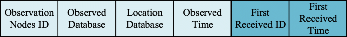
Improved format of data packet
-
(b)
“Observed Database” stores the data information observed by sensor nodes in each cycle. In the actual positioning process, we set sensors to observe the data periodically.
-
(c)
“Location Database” stores the locations of observation nodes.
-
(d)
“Observation Time” is defined as the time when the observation data is received. It is assumed that sensor will broadcast the data packet immediately after observing the data [31].
-
(e)
“First Received ID” is defined as the ID of the first node that received data packet among those neighbor nodes that stored in the packet.
-
(f)
“First Receive Time” stores the time when the “First Receive ID” received from data packet.

In all UWSN applications, the four fields, (a), (b), (c), and (d), are indispensable. This paper improves the existing data format. Two fields, (e) and (f), are added to correct the data position so as to obtain more accurate positioning results.
After several data transfers, the data will be grouped and sent to base station. Then, base station classifies the received data packets according to “Observation Time,” and these data packets with the same or close to the “Observation Time” will be classified into the same group.
As shown in Table 1, this example groups the received data packets whose “observation time” is the second moment, when the number of data packets reaches saturation or reaches a predetermined time of data transmission, base station will initiate the data position correction.
Figure 3 shows the structure of the packet grouping in Table 1. The data information of sensor nodes and beacon nodes is in the same data packet. The “data transmission node” and “data receiving node” in the packet are adjacent to each other. We represent them as node a and node b and use a set of undirected edges to represent their relationship in the data structure diagram of IO-DPC.

The packet structure diagram corresponding to Table 1
3.3 IO-DPC data initialization
Assuming that the nodes are clock synchronized, the ToA technology is used to send data packets between nodes and include the information of transmission time. The calculation of the transmission distance is shown in Eq. (1).
where v denotes the acoustic velocity in sea water, v=1500m/s, and ΔtToA represents arrival time. However, there is a transmission delay of sound waves in seawater and the transmission rate is constantly changing. The transmission delay makes the distance error larger measured by ToA. Equations (2) and (3) describe the relationship between the authentic distance and the distance measured by ToA.
where dreal represents the true distance between two sensor nodes, ξ represents the error between Gaussian distribution simulation and the distance measured by ToA, ρ indicates positional parameter, and σ indicates scale parameter.
Each node in IO-DPC data structure diagram is an entry in the packet grouping table. In the initial rough positioning stage, in each self-positioning period Pself, the position of node by self-positioning will be set as the position of data packet. The confidence of the position of the data packet in each data observation period Pdata is set to 1/(1+T), where T is the time of receiving observation data, and the range of T is 0 to Pself/(Pdata−1). With the increase in positioning time and energy consumption during data transmission, Pself will even be a multiple of Pdata, so the accuracy of positioning will decrease accordingly. The ID of the two neighbor nodes are respectively represented as aid and bid; dToA(aid,bid) represents the ToA distance between nodes and their neighbors. Its confidence coefficient c(aid,bid) is shown in Eq. (4).
where R indicates the communication radius of nodes. When measured distance is greater than R, the confidence coefficient of ToA distance is 0, because it is unreasonable that the measured distance greater than communication radius.
As shown in Eq. (5), the Euclidean distance dEuc(a,b) between neighboring nodes of “data transmission node” and “data reception node” is calculated according to the positions of the two nodes; dEuc(a,b) will be updated when the position of data package has been updated.
For example, B1, B2, and B3 are beacon nodes in Fig. 4, and their position coordinates are B1 (58.26, 28.86), B2 (54.36, 32.40), and B3 (52.36, 41.86). Their confidence is 1, because the position of the beacon node is known, so it is considered to be very accurate. The list of their neighbors is empty because they do not need other nodes to correct their positions. In this example, the data observation period Pdata is set to 1. Since the self-localization time of the last sensor is 0 and the observation time of data packet is the second time, the confidence of data packet position is 0.33. The neighbor nodes of node 9 include node 1, node 2, node 4, node 6, and node 8. Node 1 first received the data packet at time 2.0066. In this case, we set the communication radius to 13. Therefore, the ToA distance between node 1 and node 9 is 9.900, and the confidence coefficient of ToA distance is 0.238.

The shift vector is determined in two cases. adToA(Naux,refid)>dEuc(Naux,refid). bdToA(Naux,refid)<dEuc(Naux,refid)
4 Positioning phase of IO-DPC
IO-DPC positioning technology proposed in this paper includes two parts: rough positioning stage performed by the node itself and data position correction stage performed by base station.
4.1 Rough positioning of sensor nodes
4.1.1 Particle swarm optimization
Particle swarm optimization (PSO) algorithm [32] is a simulation of simplified swarm agent model. The algorithm can make particles fly to the solution space and land at the best position to get the optimal solution. PSO algorithm selects the number of initial random particles to be m, and each particle represents a solution. Each particle has position and velocity information and an adaptive value determined by objective function to judge the particle quality. It is supposed that the absolute position coordinate of the ith particle is Xi=[xi1,xi2,⋯,xim] and the velocity is vi=[vi1,vi2,⋯,vim]. In each iteration, particles update themselves by tracking the individual optimal solution Ibest and the global optimal value Gbest. When these two optimal values are found, particles update their speed and position according to Eqs. (6) (7) (8).
where ω denotes the inertial weight, and iter represents the number of iterations. φ1 represents learning factor, and γ1 is the random number between 0 and 1.
4.1.2 Iteration
The optimization starts from common nodes around the initial beacon node. If there are three or more optimized nodes or initial beacon nodes around a certain node, the optimization of positioning of this node can be achieved. When a node is located and optimized, it is converted into a localized beacon node to participate in the optimization of positioning of other nodes. This process is followed by iteration until all nodes have been optimized or the number of nodes that have not been optimized no longer increases. If there are not more than three beacon nodes around, it cannot be optimized. After all other nodes are located and optimized, redetect the number of optimized points around nodes that have not been optimized. If there are three or more, it will be located according to the above method, and less than three cannot be located.
4.2 Data packet position correction
4.2.1 Search for auxiliary nodes
When a node’s confidence coefficient is less than the specified threshold, the node will be considered as a correctable candidate node. As the number of candidate nodes increases, base station will select one of them to determine whether it is eligible to become an auxiliary node Naux. For example, in the example shown in Fig. 4, base station will first select node 9 because it has enough neighbors. Base station calculates the credibility of each neighbor of node 9. The credibility is calculated by Eq. (9), and the four most reliable neighbors can be quickly selected as the reference node refid.
In order to check whether these reference nodes are trusted enough to modify position of the data package, base station recalculates confidence coefficient of the corrected node 9 of the reference node according to Eqs. (10) and (11).
where α represents the adjustment parameter; it is the weight used to adjust the confidence coefficient of ToA distance. When the measured distance is more precise, the value of α is greater than 0.5. System uses the average confidence coefficient of three reference nodes as the confidence coefficient of Naux and calculates the position of Naux according to the three reference nodes.
If the value of cpos(Naux) is greater than cpos(refid), the node will be defined as an auxiliary Naux; the position will be calculated according to the scheme introduced in the following portion. If not, the base station will skip the node, re-select the other candidate for calculation, and use the recursive method to select auxiliary node. When there is no candidate node, the recursive selection of auxiliary nodes will be stopped. Table 2 shows the results of selecting auxiliary nodes.
4.2.2 Calculate the location of auxiliary node
IO-DPC uses Eq. (12) to calculate the displacement vector of auxiliary node.
where α represents the adjustment parameter, which has been given in Eq. (11). The determination of shift vector also requires the following two cases.
-
i.
When ToA distance between auxiliary node and reference node is greater than its Euclidean distance [33], that is, dToA(Naux,refid)>dEuc(Naux,refid). As Fig. 4a shows, under the circumstances, auxiliary node 9 will be shifted in the direction shown in the figure.
-
ii.
When ToA distance between auxiliary node and reference node is less than its Euclidean distance, that is, dToA(Naux,refid)<dEuc(Naux,refid). As Fig. 4b shows, on this occasion, auxiliary node 9 will be shifted to a position closer to its reference node (node 6).
According to the above method, each reference node around the auxiliary node will generate a shift vector. The position of the auxiliary node Naux after data correction is denoted as \(N^{\prime }_{{aux}}\). As shown in Fig. 5, also taking node 9 as an example, the position after data correction is determined by the total force of the three displacement vectors shown in Fig. 5. It is computed according to Eq. (13).

Results of data position correction of the auxiliary node
When there are no candidate nodes in positioning system, the average and variance of the confidence coefficient of all nodes will be calculated at this moment. When mean variance of cpos(aid) is less than the set threshold θc, the process of data position correction of IO-DPC has been completed. Table 3 shows the final results of data position correction.
4.3 Ocean current model
In UWSNs, sensor nodes will move with ocean currents, which affects the accuracy of positioning. Ocean currents have the characteristics of continuously changing movement speed and semi-periodic motion, and their motion characteristics are correlated in space and time [34], as shown in Fig. 6. Therefore, the ocean current model is used to describe the motion of nodes.

Relationship between coastal velocity and time. a East-west velocity. b North-south velocity
Considering that there are many factors that affect the movement of ocean currents in seawater and the positioning process is complicated, therefore, underwater motion model is difficult to establish. The ocean current motion model used in the literature [35] is adopted here. It is assumed that underwater acoustic nodes are only affected by jet and vortex flow, and they only move with the current in the same flat. The speed of node movement is continuously changing. The node motion model is shown by Eqs. (14) and (15).
where q indicates the number of jets per unit length, c indicates the angular velocity, D(t) represents the width of ocean current, E represents the average width, μ denotes the amplitude of modulation, and ϖ denotes the frequency of modulation.
5 Experimental and simulation analysis
5.1 Experimental deployment
The performance evaluation of IO-DPC system is carried out in this section. The experimental parameters are shown in Table 4. The area of the simulated experimental scene is 120m×120m×120m. The number of buoy nodes, beacon nodes, and sensor nodes deployed in the experimental area are 25, 50, and 425 respectively. The average data calculation time of 500 nodes is about 3 s, communication radius is 23 m, data observation period is set to 1 s, and the threshold is set to 0.001. It can be seen from the existing underwater ranging technology that the measured distance between nodes is subject to average value as actual distance. The normal distribution with a standard deviation of 2% of the actual distance is reasonable [36]. The result of the experimental simulation is the average value of 100 simulation experiments. The smart device used for the experiment is Lenovo G50-80, Intel (R) Core (TM) i5-5200U.
5.2 Experimental results and analysis
5.2.1 Positioning error
Figure 7 shows the experimental results of positioning errors varying with the modulation amplitude in ocean current model over 10 data observation periods. In the process of experimental simulation, the self-positioning period is set to 10 times of data correction period, so as to measure the cumulative results of positioning errors within 10 periods. For the parameters of ocean current model, we set the amplitude of modulation to 2, 3, 4, and 5 respectively. At this time, the corresponding ocean current velocities are 0.92 m/s, 1.68 m/s, 2.06 m/s, and 3.32 m/s respectively. It can be seen from the results that errors will accumulate with the increase of data observation period. And the meander width of ocean current model will increase as the modulation amplitude increases. The movement speed of sensor node will gradually increase, and the density of nodes will gradually decrease. Therefore, the positioning error becomes an increasing trend. However, in four cases, the errors within 10 cycles are controlled within the range of 0.85R. It indicates that the positioning performance of IO-DPC technology is relatively good.

Change of positioning error with current amplitude during 10 periods
5.2.2 Location coverage
Location coverage indicates the proportion of positioned nodes to all nodes, with ζ=npos/n×100%, where npos indicates the number of ordinary nodes that have been located, and n denotes the number of all ordinary nodes. Figure 8 shows the experimental results of location coverage varying with the modulation amplitude in ocean current model over 10 data observation periods. It can be seen that with the increase of meandering width of ocean current, the moving speed of sensor nodes gradually increases. The density of nodes gradually decreases, so the location coverage shows a decreasing trend. However, the location coverage of the nodes in the four cases is controlled above 98%. It shows that the stability of IO-DPC technology is high.

Change of location coverage with current amplitude during 10 periods
5.2.3 Proportion of beacon nodes
We compared the influence of proportion of beacon nodes on positioning error in 10 periods by taking the beacon nodes at initial experimental deployment as a reference. The simulation results are shown in Fig. 9. In ocean current model, the modulation amplitude is set to μ=5. It can be seen that the more beacon nodes, the smaller positioning error and the higher positioning accuracy. For example, when beacon nodes account for 10% of total nodes, the cumulative positioning error in 10 periods is about 0.9R, and when beacon nodes account for 20%, the cumulative positioning error is about 0.65R. It shows that in sparse underwater wireless sensor networks, we can increase positioning accuracy by increasing the proportion of beacon nodes. For all range-based underwater positioning technologies, positioning accuracy will increase as the proportion of beacon nodes increases. However, when the number of beacon nodes reaches saturation, adding too many beacon nodes will lead to the increase of communication cost.

Change of positioning error with the proportion of beacon nodes in 10 periods
5.2.4 Iteration
Four iterations are set for IO-DPC system. Figure 10 shows the position estimation results under different iteration times. (a) reflects the positioning result when the number of iteration is 1, (b) reflects the positioning result when the number of iteration is 4. The number of iterations can continue to increase, but it will lead to an increase in workload, so 4 iterations is optimal in this experiment. It is found that the average estimation error obtained is dynamic after four iterations, and the average positioning error is about 0.07R–0.15R. The positioning accuracy has been significantly improved after iterative optimization.

Position estimation results at different iteration times. a The number of iterations is 1. b The number of iterations is 4
5.2.5 Comparison with other systems
IO-DPC technology was compared with two other typical technologies: large underwater network localization scheme (LSLS) [37] and underwater layered localization scheme (LSHL) [38]. In the simulation experiment, the self-positioning period of the node is set to 2 times of data correction period. Figures 11 and 12 clearly show the impact of node migration on positioning performance and communication cost in underwater wireless sensor networks. The simulation results show that positioning errors of all schemes increase with the increase of node moving speed. IO-DPC corrects the position of data packets more accurately and reduces the communication cost. This is because the data position correction of IO-DPC is performed on base station. Therefore, the time for sending positioning information is extended, thereby reducing the communication cost.

Comparison of positioning error between IO-DPC and the other two technologies

Comparison of average communication cost between IO-DPC and the other two technologies
6 Conclusion
Aiming at the complex underwater dynamic positioning environment and the message propagation delay, excessive positioning error, and excessive positioning time caused by the mobility of sensor nodes, this paper proposed an underwater wireless sensor network localization method based on iterative optimization and data position correction (IO-DPC), which compensated for the deviation of distance estimation caused by the continuous self-positioning of nodes. Firstly, the particle swarm optimization algorithm was used to carry out self-positioning of nodes in the rough positioning stage, and multiple iteration optimization was performed. Then, ToA technology was used to achieve point-to-point timing transmission of data packets on the basis of assuming clock synchronization between nodes. Finally, after receiving the data packet containing position information of node’s self-positioning, the data position correction was performed by base station. In addition, an ocean current model was designed to test the performance of IO-DPC in different underwater simulation environments. Experimental results show that IO-DPC has higher positioning accuracy and lower communication cost than other schemes, which verifies the effectiveness of IO-DPC. Future research will consider simulation in an obstacle space with irregular underwater activities.
Abbreviations
- UWSNs:
-
Underwater wireless sensor networks
- IO-DPC:
-
Iterative optimization and data position correction
- UUV:
-
Unmanned underwater vehicles
- AUV:
-
Autonomous underwater vehicles
- TWSNs:
-
Terrestrial wireless sensor networks
- ToA:
-
Time of arrival
- PSO:
-
Particle swarm optimization
References
J. Heidemann, M. Stojanovic, M. Zorzi, Underwater sensor networks: applications, advances and challenges. Philos. Trans. R. Soc. A Math. Phys. Eng. Sci.370:, 158–175 (2012).
N. Mohamed, I. Jawhar, J. Al-Jaroodi, L. Zhang, Sensor network architectures for monitoring underwater pipelines. Sensors. 11(11), 10738–10764 (2011).
Q. Fengzhong, W. Shiyuan, W. Zhihui, L. Zubin, A survey of ranging algorithms and localization schemes in underwater acoustic sensor network. China Commun.13(3), 66–81 (2016).
G. Han, S. Shen, H. Song, T. Yang, W. Zhang, A stratification-based data collection scheme in underwater acoustic sensor networks. IEEE Trans. Veh. Technol.67(11), 10671–10682 (2018).
Y. Cao, N. Zhao, F. R. Yu, M. Jin, Y. Chen, J. Tang, V. C. Leung, Optimization or alignment: secure primary transmission assisted by secondary networks. IEEE J. Sel. Areas Commun.36(4), 905–917 (2018).
H. P. Tan, R. Diamant, W. K. G. Seah, M. Waldmeyer, A survey of techniques and challenges in underwater localization. Ocean Eng.38(14-15), 1663–1676 (2011).
M. Beniwal, R. Singh, Localization techniques and their challenges in underwater wireless sensor networks. Int. J. Comput. Sci. Inf. Technol.5:, 4706–4710 (2014).
P. Thulasiraman, K. A. White, Topology control of tactical wireless sensor networks using energy efficient zone routing. Digit. Commun. Netw.2(1), 1–14 (2016).
A. Pughat, V. Sharma, Performance analysis of an improved dynamic power management model in wireless sensor node. Digit. Commun. Netw.3:, 19–29 (2017).
X. Liu, M. Jia, X. Zhang, W. Lu, A novel multichannel Internet of things based on dynamic spectrum sharing in 5G communication. IEEE Internet Things J.6(4), 5962–5970 (2019).
X. Liu, X. Zhang, NOMA-based resource allocation for cluster-based cognitive industrial Internet of Things. IEEE Trans. Ind. Inform.16(8), 5379–5388 (2019).
J. T. Zhou, H. Zhao, X. Peng, M. Fang, Z. Qin, R. S. M. Goh, Transfer hashing: From shallow to deep. IEEE Trans. Neural Netw. Learn. Syst.29(12), 6191–6201 (2018).
Y. Zhang, J. Liang, S. Jiang, W. Chen, A localization method for underwater wireless sensor networks based on mobility prediction and particle swarm optimization algorithms. Sensors. 16(2), 212 (2016).
V. Garg, M. Jhamb, A review of wireless sensor network on localization techniques. Int. J. Eng. Trends Technol.4:, 1049–1053 (2013).
T. J. S. Chowdhury, C. Elkin, V. Devabhaktuni, D. B. Rawat, J. Oluoch, Advances on localization techniques for wireless sensor networks: A survey. Comput. Netw.110:, 284–305 (2016).
G. Han, H. Xu, T. Q. Duong, J. Jiang, T. Hara, Localization algorithms of wireless sensor networks: a survey. Telecommun. Syst.52:, 2419–2436 (2013).
Z. Zhou, Z. Peng, J. H. Cui, Z. Shi, A. Bagtzoglou, Scalable localization with mobility prediction for underwater sensor networks. IEEE Trans. Mob. Comput.10(3), 335–348 (2011).
G. Zhu, R. Jiang, L. Xie, Y. Chen, in 26th Chinese Control and Decision Conference (2014 CCDC). A distributed localization scheme based on mobility prediction for underwater wireless sensor networks (IEEE, 2014), pp. 4863–4867.
D. Mirza, C. Schurgers, in Proceedings of the OCEANS. Collaborative localization for fleets of underwater drifters (IEEEVancouver, Canada, 2007), pp. 1–6.
Y. Zhou, K. Chen, J. He, J. Chen, A. Liang, in 2009 11th IEEE International Conference on High Performance Computing and Communications. A hierarchical localization scheme for large scale underwater wireless sensor networks (IEEE, 2009), pp. 470–475.
X. Cheng, H. S. H. Shu, Q. Liang, in International Conference on Wireless Algorithms, Systems and Applications (WASA 2007). A range-difference based self-positioning scheme for underwater acoustic sensor networks (IEEE, 2007), pp. 38–43.
W. Biao, L. Chao, Z. Zhi, Z. Qingjun, DOA estimation based on compressive sensing method in micro underwater location platform. Appl. Math. Inf. Sci. 9(3), 1557 (2015).
J. Yan, Z. Xu, X. Luo, C. Chen, X. Guan, Feedback-based target localization in underwater sensor networks: a multisensor fusion approach. IEEE Trans. Signal Inf. Process. Netw.5(1), 168–180 (2019).
S. Lee, K. Kim, Localization with a mobile beacon in underwater acoustic sensor networks. Sensors. 12(5), 5486–5501 (2012).
X. Cheng, H. Shu, Q. Liang, D. H. -C. Du, Silent positioning in underwater acoustic sensor networks. IEEE Trans. Veh. Technol.57(3), 1756–1766 (2008).
M. Erol, L. F. M. Vieira, M. Gerla, in Proceedings of the Second ACM International Workshop on Underwater Networks. Localization with Dive’N’Rise (DNR) beacons for underwater acoustic sensor networks (ACMNew York, 2007), pp. 97–100.
C. Bechaz, H. Thomas, in Proceedings of the 5th Europe Conference on Underwater Acoustics. GIB system: the underwater GPS solution, (2000).
T. C. Austin, R. P. Stokey, K. M. Sharp, in OCEANS 2000 MTS/IEEE Conference and Exhibition. Conference Proceedings (Cat. No. 00CH37158). PARADIGM: a buoy-based system for AUV navigation and tracking (IEEE, 2000), pp. 935–938.
J. Liu, Z. Wang, J. H. Cui, S. Zhou, B. Yang, A joint time synchronization and localization design for mobile underwater sensor networks. IEEE Trans. Mob. Comput.15(3), 530–543 (2015).
J. Liu, Z. Zhou, Z. Peng, J. -H. Cui, M. Zuba, L. Fiondella, Mobi-sync: efficient time synchronization for mobile underwater sensor networks. IEEE Trans. Parallel Distrib. Syst.24(2), 406–416 (2013).
D. Mirza, C. Schurgers, in Proceedings of the 3rd ACM International Workshop on Underwater Networks. Motion-aware self-localization for underwater networks, (2008), pp. 51–58.
S. Yu, C. Eberhart, in Proceedings of the 7th International Conference on Evolutionary Programming VII. Parameter selection in particle swarm optimization (Springer-VerlagBerlin Heidelberg, 1998), pp. 591–600.
D. Niculescu, B. Nath, in Proceedings of the 22nd Annual Joint Conference on the IEEE Computer and Communications Societies (INFOCOM’03). Ad hoc positioning system (APS) using AOA (San Francisco, Calif, USA, 2003), pp. 1734–1743.
S. P. Beerens, H. Ridderinkhof, J. T. F. Zimmerman, An analytical study of chaotic stirring in tidal areas. Chaos, Solitons Fractals. 4(6), 1011–1029 (1994).
A. Caruso, F. Paparella, L. F. M. Vieira, Luiz F. M., M. Erol, M. Gerla, in Proceedings of the 27th IEEE Communications Society Conference on Computer Communications (INFOCOM’08). The meandering current mobility model and its impact on underwater mobile sensor networks (IEEEPhoenix, Ariz, USA, 2008), pp. 221–225.
L. Xin, Z. Xiangping, L. Weidang, C. Wu, QoS-guarantee resource allocation for multibeam satellite industrial Internet of Things with NOMA. IEEE Trans. Ind. Inform., 1–10 (2019).
Z. Zhou, J. H. Cui, S. Zhou, Efficient localization for large-scale underwater sensor networks. Ad Hoc Netw.8(3), 267–279 (2010).
G. Han, A. Qian, C. Zhang, Y. Wang, J. J. P. C. Rodrigues, Localization algorithms in large-scale underwater acoustic sensor networks: a quantitative comparison. Int. J. Distrib. Sensor Netw.10(3), 379382 (2014).
Acknowledgements
The work was supported by the National Natural Science Foundation of China (61771186), Postdoctoral Research of Heilongjiang Province (LBH-Q15121), Undergraduate University Project of Young Scientist Creative Talent of Heilongjiang Province (UNPYSCT-2017125), and Postgraduate Innovative Research Project of Heilongjiang University (YJSCX2020-164HLJU).
Publisher’s Note
Springer Nature remains neutral with regard to jurisdictional claims in published maps and institutional affiliations.
Authors’ contributions
DyQ and XxW conceptualized the idea and designed the experiments. XxW contributed in writing and draft preparation and DyQ supervised the research. All authors read and approved the final manuscript.
Funding
The funding was supported by the National Natural Science Foundation of China (61771186), Postdoctoral Research of Heilongjiang Province (LBH-Q15121), Undergraduate University Project of Young Scientist Creative Talent of Heilongjiang Province (UNPYSCT-2017125), and Postgraduate Innovative Research Project of Heilongjiang University (YJSCX2020-164HLJU).
Availability of data and materials
Not applicable.
Competing interests
The authors declare that they have no competing interests.
Author information
Authors and Affiliations
Corresponding author
Rights and permissions
Open Access This article is licensed under a Creative Commons Attribution 4.0 International License, which permits use, sharing, adaptation, distribution and reproduction in any medium or format, as long as you give appropriate credit to the original author(s) and the source, provide a link to the Creative Commons licence, and indicate if changes were made. The images or other third party material in this article are included in the article’s Creative Commons licence, unless indicated otherwise in a credit line to the material. If material is not included in the article’s Creative Commons licence and your intended use is not permitted by statutory regulation or exceeds the permitted use, you will need to obtain permission directly from the copyright holder. To view a copy of this licence, visit http://creativecommons.org/licenses/by/4.0/.
About this article

Cite this article
Wang, X., Qin, D., Zhao, M. et al. UWSNs positioning technology based on iterative optimization and data position correction. J Wireless Com Network 2020, 158 (2020). https://doi.org/10.1186/s13638-020-01771-9
Received:
Accepted:
Published:
DOI: https://doi.org/10.1186/s13638-020-01771-9