Oscillatory-Precessional Motion of a Rydberg Electron Around a Polar Molecule

Physics Department, 380 Duncan Drive, Auburn University, Auburn, AL 36849, USA
Symmetry 2020, 12(8), 1275; https://doi.org/10.3390/sym12081275
Submission received: 3 July 2020
/
Revised: 10 July 2020
/
Accepted: 10 July 2020
/
Published: 2 August 2020
(This article belongs to the Special Issue Atomic Processes in Plasmas and Gases: Symmetries and Beyond)
Abstract
:We provide a detailed classical description of the oscillatory-precessional motion of an electron in the field of an electric dipole. Specifically, we demonstrate that in the general case of the oscillatory-precessional motion of the electron (the oscillations being in the meridional direction (θ-direction) and the precession being along parallels of latitude (φ-direction)), both the θ-oscillations and the φ-precessions can actually occur on the same time scale—contrary to the statement from the work by another author. We obtain the dependence of φ on θ, the time evolution of the dynamical variable θ, the period Tθ of the θ-oscillations, and the change of the angular variable φ during one half-period of the θ-motion—all in the forms of one-fold integrals in the general case and illustrated it pictorially. We also produce the corresponding explicit analytical expressions for relatively small values of the projection pφ of the angular momentum on the axis of the electric dipole. We also derive a general condition for this conditionally-periodic motion to become periodic (the trajectory of the electron would become a closed curve) and then provide examples of the values of pφ for this to happen. Besides, for the particular case of pφ = 0 we produce an explicit analytical result for the dependence of the time t on θ. For the opposite particular case, where pφ is equal to its maximum possible value (consistent with the bound motion), we derive an explicit analytical result for the period of the revolution of the electron along the parallel of latitude.
1. Introduction
An electron in the field of an electric dipole is the second most fundamental problem in atomic/molecular physics after the hydrogen atom—especially if the distance of the electron from the dipole is much larger than the dimension of the dipole, so that the dipole can be considered point-like. Theoretical studies of this fundamental system started as early as in 1947, when Fermi and Teller [1] investigated this problem in relation to the situation where a muon is slowly moving through a hydrogen atom. In the intervening years, many works have been published on this subject—see, e.g., paper [2] and references therein.
As for the classical motion, which is appropriate for a Rydberg electron in the field of an electric dipole, there were the following two theoretical studies for the case of the finite electric dipole (to the best of our knowledge). In 1968, Turner and Fox [3] considered the problem analytically in the elliptical coordinates (ξ, η, φ). They showed that for any finite size of the dipole, the bound motion exists in some region (ξmin < ξ < ξmax, ηmin < η < ηmax). The motion occurs inside a torus created by the revolution (about the dipole axis) of the two limiting ellipses, corresponding to ξ = ξmin and ξ = ξmax, and of the two limiting parabolas, corresponding to η = ηmin and η = ηmax.
In 2013, Kryukov and Oks [4] started by analytically considering circular orbits of a negative charge in the field of a finite dipole, when the orbital plane was perpendicular to the dipole axis; they used the cylindrical coordinates. (We note that as the application, the authors of paper [4] chose the finite dipole to be made by stationary proton and electron, while the negative charge moving in the field of this dipole was a muon; however, their analytical results are totally applicable to the motion of an electron in the field of any finite dipole.) They showed that stable circular orbits exist if the size of the dipole is greater or equal to some finite value (this value turned out to be the same as in many quantal studies of this system—see, e.g., paper [2] and references therein). Further, the authors of paper [4] went beyond the circular orbits and presented analytically a stable conic-helical motion of the electron in the field of the finite dipole: the helical orbit is confined to the surface of a right frustum of a cone coaxial with the dipole.
It is worth mentioning that obtaining the analytical results in papers [3,4] was possible because the general problem of the motion of a charged particle in the field of two stationary Coulomb centers (the problem, of which the motion of a charge in the field of a finite dipole is a particular case) is characterized by higher than geometrical (i.e., algebraic) symmetry. The symmetry is manifested by the presence of an additional conserved quantity: the projection of the super-generalized Runge–Lenz vector on the axis connecting the stationary charges [5].
As for the classical motion of a charged particle in the field of a point-like electric dipole, there were the following three theoretical studies (to the best of our knowledge). In 1968, Fox [6] treated this problem analytically and showed that the bound motion is possible only for the energy E = 0 and it is confined to a sphere. The author of paper [6] obtained the results in the form of quadratures, i.e., expressed them in terms of integrals, but without performing the integration and without a qualitative description of the motion (some details from paper [6] are reproduced in the next section of the present paper).
In 1995, Jones [7] derived analytical results for a semicircular orbit along a meridian on a sphere, to which the motion is confined (confined according to Fox result [6]). He considered the moving particle to be positively charged and pointed out that its motion is identical to the motion of a pendulum: the potential of a simple pendulum is identical to the potential of the dipole at a constant radius.
In 1996, McDonald [8] focused at two types of circular (or semicircular) orbits. One type was the same as that presented by Jones [7]. Another type was a circular orbit along a certain parallel of latitude. For the general case, McDonald [8] reproduced some analytical results from Fox’s paper [6] (without referring to that paper) and then mentioned that in general the motion should consist of large oscillations with respect to the polar angle θ combined with a slow precession about the z-axis (the z-axis being the dipole axis).
In the present paper we start where Fox stopped in paper [6]. We provide a detailed classical description of the oscillatory-precessional motion of an electron in the field of an electric dipole. Specifically, we demonstrate that in the general case of the oscillatory-precessional motion of the electron (the oscillations being in the meridional direction (θ-direction) and the precession being along parallels of latitude (φ-direction)), both the θ-oscillations and the φ-precessions can actually occur on the same time scale, so the statement to the contrary from work [8] is incorrect.
We obtain the dependence of φ on θ in the form of a one-fold integral in the general case and illustrate it pictorially. We also derive an explicit analytical result for φ(θ) for relatively small values of the projection pφ of the angular momentum on the axis of the electric dipole.
For the particular case of pφ = 0 we produce an explicit analytical result for the dependence of the time t on θ. For the opposite particular case, where pφ is equal to its maximum possible value (consistent with the bound motion), we derive an explicit analytical result for the period of the revolution of the electron along the parallel of latitude.
We obtain the time evolution of the dynamical variable θ, the period Tθ of the θ-oscillations, and the change of the angular variable φ during one half-period of the θ-motion—all in the form of one-fold integrals in the general case and illustrate it pictorially. We also produce the corresponding explicit analytical expressions for relatively small values of the projection pφ of the angular momentum on the axis of the electric dipole.
Finally, we derive a general condition for this conditionally-periodic motion to become periodic (the trajectory of the electron would become a closed curve) and then provide examples of the values of K for this to happen.
2. Classical Non-Circular Orbits
Following Fox [6], we consider an electric dipole with the dipole moment D centered at the origin. The motion of an electron in the field of the dipole is analyzed in spherical polar coordinates (r, θ, φ) with the z-axis chosen along the dipole axis, such that the positive pole points to the upper hemisphere. In this reference frame the energy has the following form:
where m and e are the mass and the absolute value of the electron charge.
E = m[(dr/dt)2 + r2(dθ/dt)2 + r2sin2θ (dφ/dt)2]/2 − eDcosθ/r2,
Due to the axial symmetry, the z-projection of the electron angular momentum Mz is conserved, as manifested by the fact that the energy, while depending on dφ/dt, does not depend on φ. Fox [6] denoted Mz as pφ because it is the generalized momentum corresponding to the dynamical variable φ:
pφ = mr2sin2θ (dφ/dt) = const.
Due to the above symmetry, the θ-motion and the φ-motion can be separated.
Fox [6] showed that the bound motion is possible only for E = 0 and r = const. Thus, the bound motion is confined to a sphere and the dynamical variables are only θ and φ.
For the θ-motion, Fox [6] derived the following differential equation:
where
(dx/dt)2 = [2eD/(mr4)](− x3 + x − K),
x = cosθ, K = pφ2/(2meD).
The corresponding equation for the φ-motion follows from Equation (2):
dφ/dt = pφ/(mr2sin2θ) = pφ/[mr2(1 − x2)].
After finding x(t) from Equation (3), one can obtain φ(t) from Equation (5).
Fox [6] noted that for the bound motion to occur, the polynomial
in Equation (3) must be positive in some range of x within the interval from −1 to 1. This polynomial has a negative minimum equal to −K − 2/33/2 at x = − 1/31/2 and a maximum equal to −K + 2/33/2 at x = 1/31/2. Obviously, for the range of the bound motion to exist, the maximum should be positive, leading to the following requirement (Fox [6]):
or equivalently (see Equation (4))
y(x) = − x3 + x − K
K < 2/33/2 = Kmax
D > 33/2pφ2/(4me).
Under the condition (7) the motion with respect to the dynamical variable x can be confined between two positive turning points, so that the bound motion occurs in the upper hemisphere, as noted by Fox [6]. We note in passing that, according to Equation (8), classical bound states exist for any value of the dipole moment D—because the generalized momentum pφ in the right side of Equation (8) can be zero. The same is true for classical bound states for any finite size of the dipole, as shown in paper [3]. In contrast, the quantum bound states exist only if the dipole moment exceeds some critical value Dmin = 0.6393148771999813 (in atomic units). This value of Dmin with the accuracy of the first 16 digits was calculated in paper [2] of 2007 (paper [2] contains references to most of the previous calculations of Dmin). However, the existence of the critical dipole moment Dmin and its first three digits were calculated as early as in 1947 by Fermi and Teller [1].
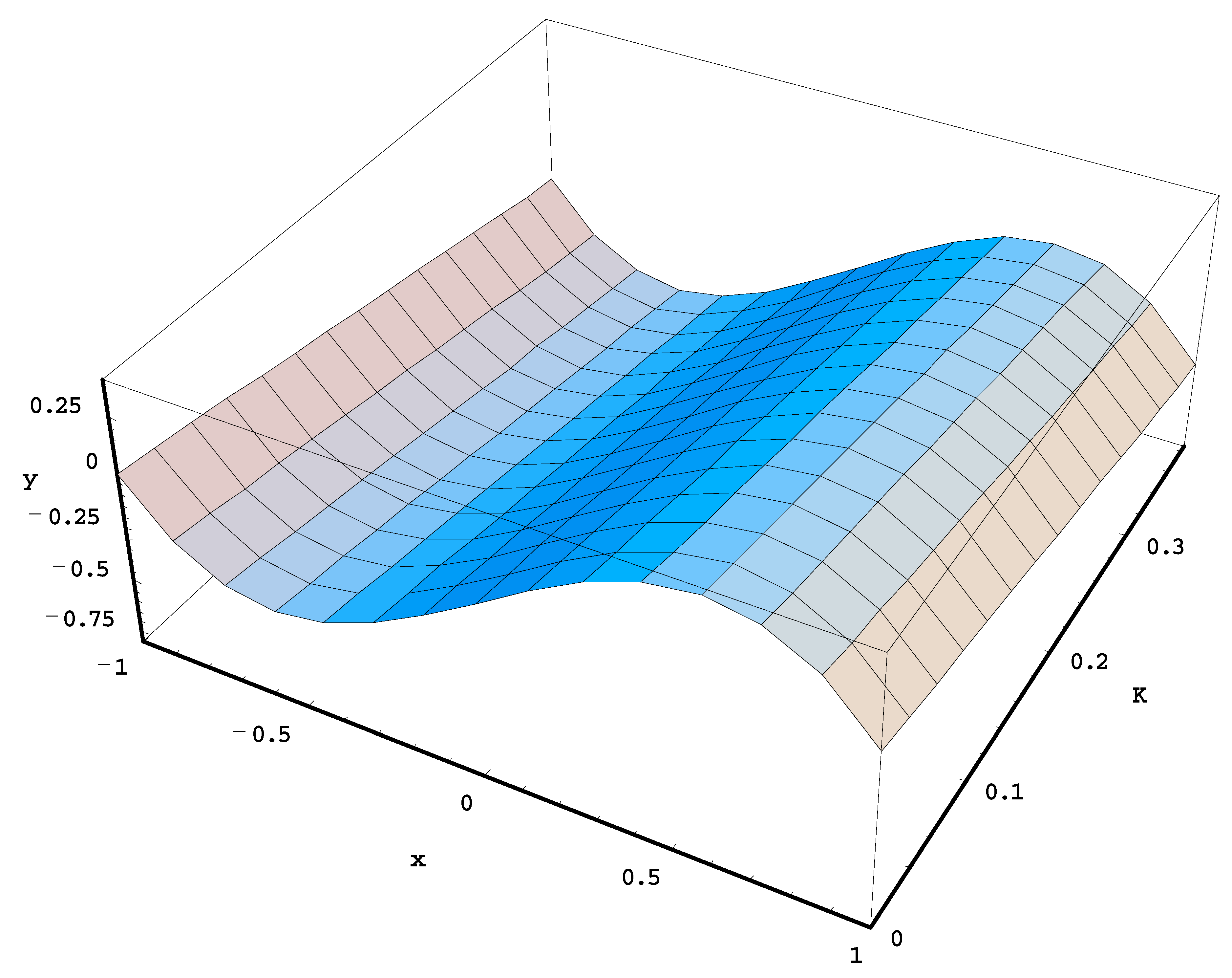
From this point on, we present new results. Figure 1 shows a three-dimensional plot of the polynomial y(x, K) as x varies from −1 to 1 and K varies from 0 to Kmax = 2/33/2. It is seen that in this range of K, the maximum value of y is positive, so that there is indeed a range of x that allows classical bound motion.
We denote positive turning points as x2 and x3 (x3 > x2. They are the real roots of the following cubic equation:
x3 − x + K = 0.
By solving Equation (9) we obtain the following explicit expressions for the turning points:
x2(K) = (−1)2/321/3/[(729K2 − 108)1/2 − 27K]1/3 − (−1)1/3[(729K2 − 108)1/2 − 27K]1/3/(21/33).
x3(K) = 21/3/[(729K2 − 108)1/2 − 27K]1/3 − [(729K2 − 108)1/2 − 27K]1/3/(21/33).
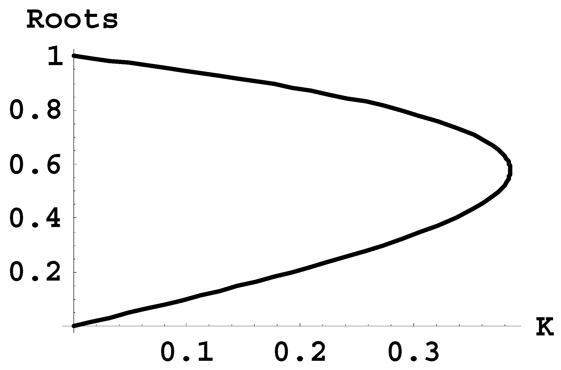
Figure 2 shows a plot of both x2(K) and x3(K), where x2(K) and x3(K) are the lower part and the upper part of the double-valued curve, respectively. The lower and upper parts intersect at K = Kmax = 2/33/2, where x2(2/33/2) and x3(2/33/2) = 1/31/2.
x2(K) and x3(K) are the lower part and the upper part of the double-valued curve, respectively.
We introduce a scaled dimensionless time τ as follows:
τ = t [2 eD/(mr4)]1/2.
Then Equation (3) can be represented in the form
dτ = ±dx/(− x3 + x − K)1/2.
(We note that Fox [6] chose only the minus sign in his Equation (12) analogous to our Equation (13); below we show that both signs should be considered.)
Now we study limiting cases. In the special case of K = Kmax = 2/33/2, there is no θ-motion: the electron follows a circular path along the parallel of latitude corresponding to cosθ = 1/31/2. The latter equation yields θ = 0.9553 rad = 54.74 degrees. (We note that McDonald [8] considered this circular motion for a positive charge, in which case cosθ = −1/31/2, so that θ = 2.1863 rad = 125.26 degrees.) From Equation (5) it follows that the electron rotates with the constant angular velocity
corresponding to the period
dφ/dt = 3pφ/(2mr2),
T = 4πmr2/(3pφ).
From Equation (4) it follows that pφ = (2KmeD)1/2, so that for K = Kmax = 2/33/2 we have pφ = 2(meD)1/2/33/4, so that Equations (14) and (15) can be rewritten as follows:
dφ/dt = 31/4[eD/(mr4] 1/2, T = (2π/31/4) [mr4/(eD)] 1/2.
In the opposite limit of K << 1, Equations (9) and (10) simplify to:
x2(K) ≈ K, x3(K) ≈ 1 − K/2.
In the special case of K = 0, i.e., pφ = 0, there is no φ-motion. The electron oscillates along a semicircle located in a meridional plane in the upper hemisphere. (This is analogous to the corresponding result by Jones [7], later reproduced by McDonald [8], for a positive charge: the only difference is that for the positive charge, the semicircular orbit is in the lower hemisphere.) Let us study this special case in more detail before proceeding to the general case.
For K = 0, Equation (13) can be integrated analytically to yield the following explicit dependence of the scaled time τ on x, i.e., the dependence of τ on cosθ:
where F(α, q) is the incomplete elliptic integral of the first kind. Despite the formal appearance of the imaginary unit i in Equation (18), the right side of Equation (18) is actually real for the range of x from 0 to 1 where the motion occurs. In particular, for x << 1, we obtain from Equation (18) the following:
τ = − {±2i F[arcsin(–x)1/2, −1]},
x ≈ ±τ/2.
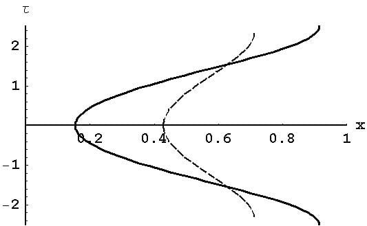
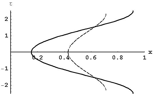
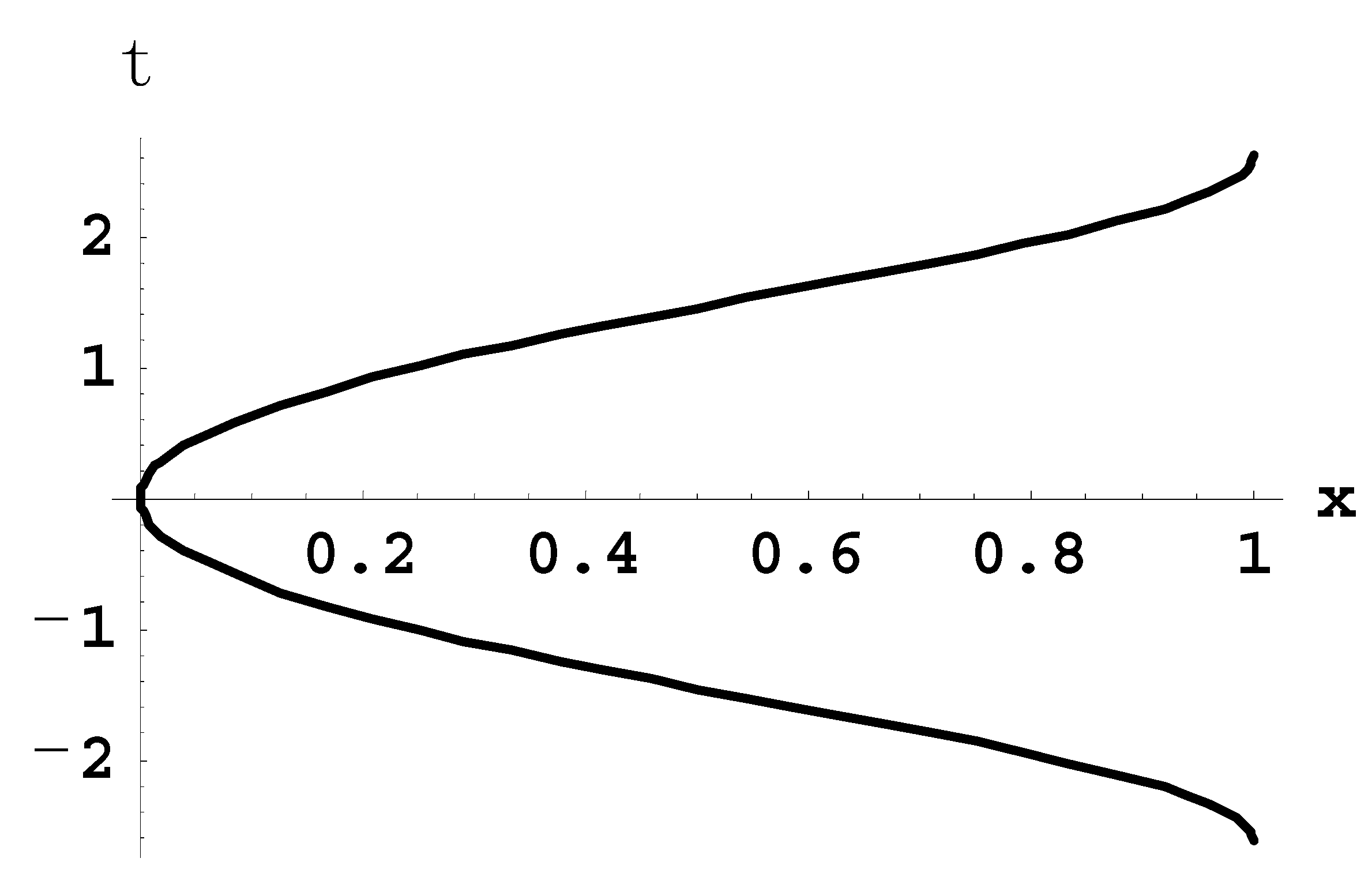
Figure 3 shows the plot of both branches of the dependence τ(x) from Equation (18): the upper and lower parts of the double-valued curve corresponds to the two different signs in the right side of Equation (18). The zero value of τ corresponds to x = 0, i.e., to θ = π/2, when the electron is at the equator of the upper hemisphere. We note that τ(±1) = ± 2.622. If we would start following the motion at τ(−1) = −2.622, i.e., when the electron is at the north pole, we would follow the lower branch of the double-valued curve in Figure 3 from x = 1 (the electron at the equator) to x = 0 at τ = 0 (the electron at the north pole), then switch to the upper branch and follow it from x = 0 to x = 1 at τ(1) = 2.622, when the electron is again at the equator. It should be emphasized that at x = 0, the geographical longitude of the electron in the upper hemisphere changes by 180 degrees.
The temporal and spatial evolutions of the electron depicted in Figure 3 obviously represent one half-cycle of its oscillations. The full period of oscillations is as follows (in terms of the scaled time):
τ0 = 4τ(1) = 10.488.
In the usual units this corresponds to the period
T = 10.488 [mr4/(2eD)]1/2.
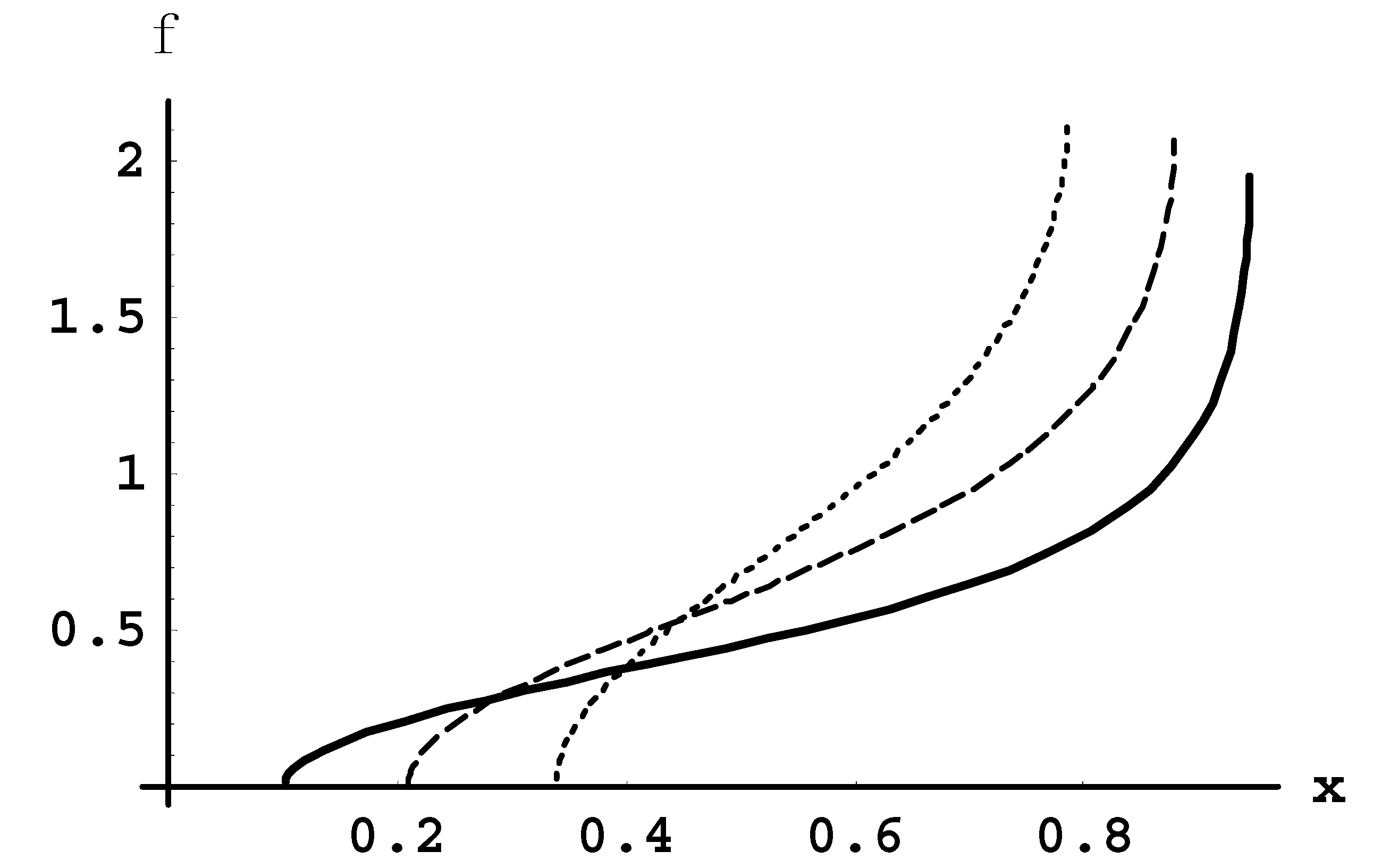
Now we come back to the general case of an arbitrary K from the interval (0, Kmax = 2/33/2). Based on Equation (13), the dependence of the scaled time τ on x (i.e., the dependence of τ on cosθ) in the general case:
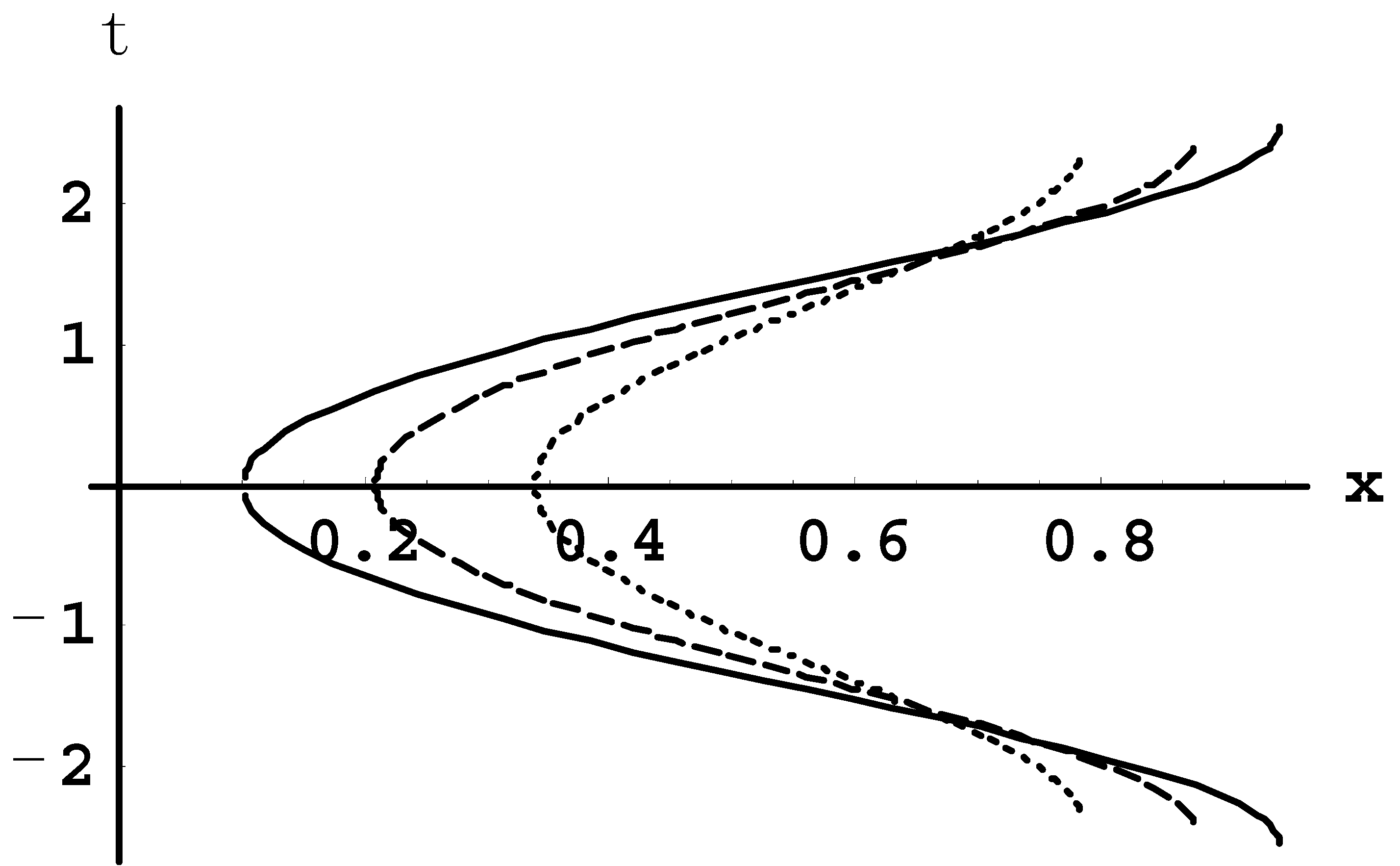
where the lower limit of the integration is the smaller of the two turning points. Figure 4 shows the evolution of the scaled time τ during one period of the θ-motion—i.e., as x varies from x2(K) to x3(K) and back to x2(K)—for K = 0.1 (solid line), K = 0.2 (dashed line), and K = 0.3 (dotted line).
For K << 1, the integral in Equation (22) can be calculated analytically. Namely, we expand this integral in Taylor series up to (including) the terms ~ K and then calculate the emerging integrals analytically to obtain the following:
τ(x, K) ≈ ±{f (x) − f [x2(K)] + Kg(x) − Kg[x2(K)]}.
Here
where 2F1(a, b, c, z) is the hypergeometric function.
f(x) = − 2i F[arcsin(–x)1/2, −1],
g(x) = [3x2− 2 − x2(1 − x2)1/2 2F1(3/4, 1/2, 7/4, x2)]/[2(x − x3)1/2]
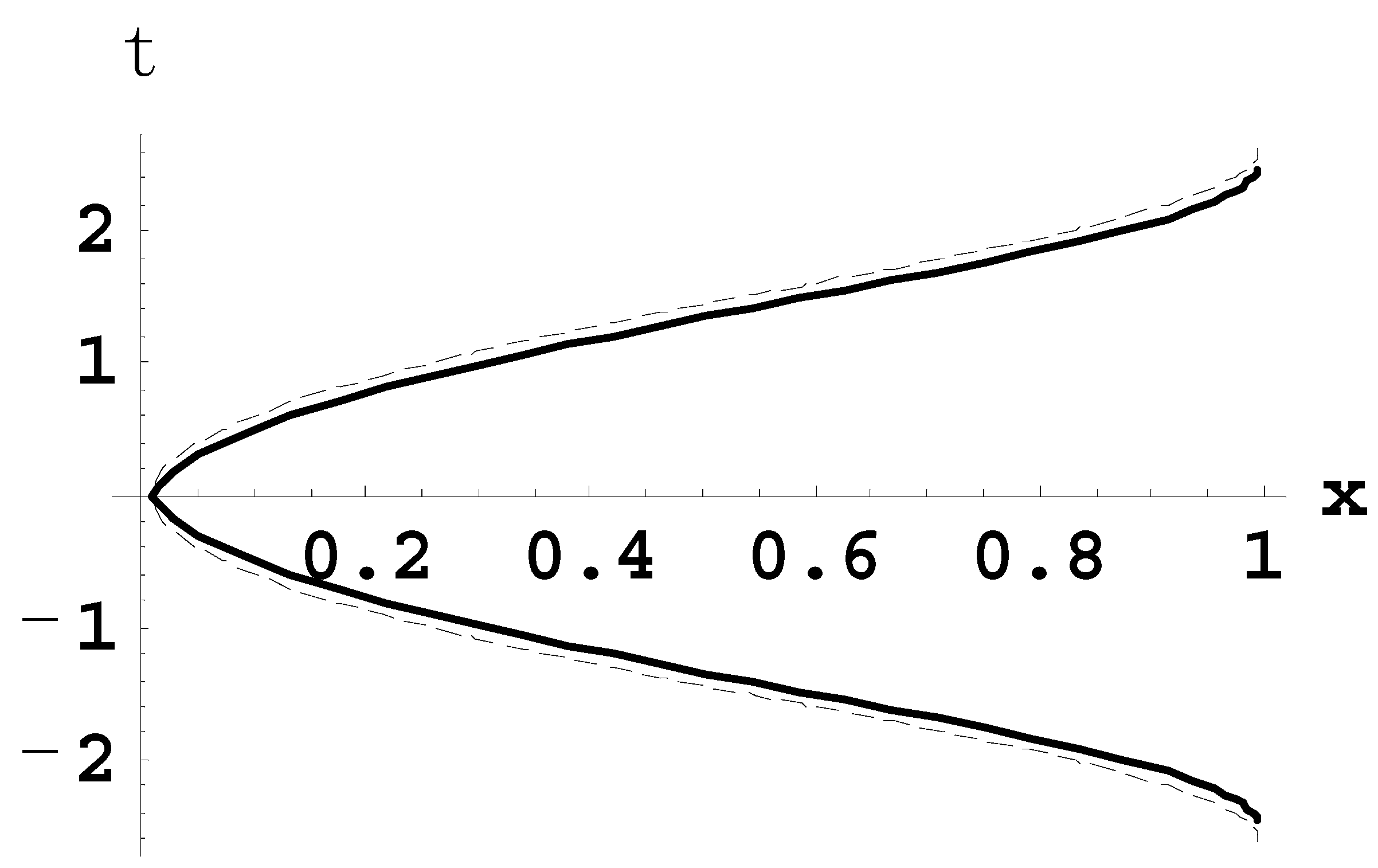
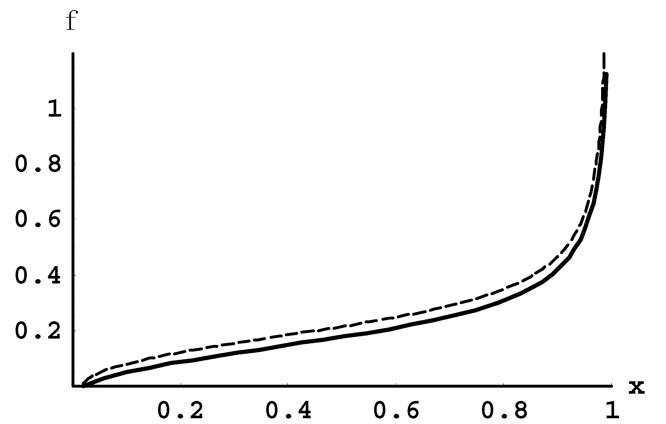
Figure 5 illustrates the accuracy of the approximate analytical result for τ(x, K) from Equation (23) for K = 0.01 (solid line) by the comparison with the corresponding exact result obtained by the numerical integration in Equation (22) (dashed line). It can be seen that the accuracy of the analytical result is very good.
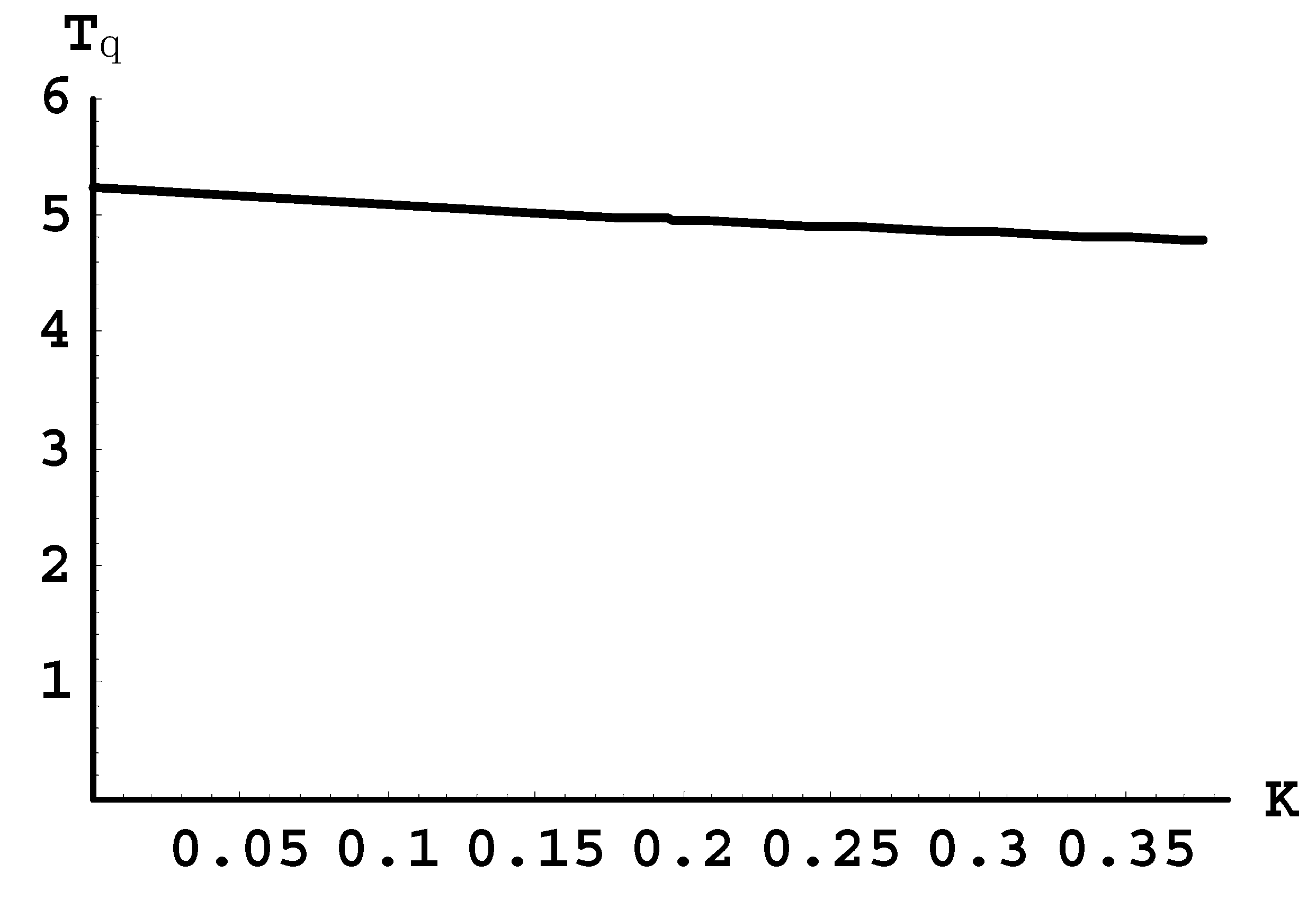
Now we calculate the scaled period Tθ of the θ-motion. It is calculated by the following formula (in units of mr4/(2eD)):
The dependence of the scaled period Tθ on K is shown in Figure 6.
For K << 1, an explicit analytical result for the scaled period of the θ-motion is as follows:
where functions f and g are defined by Equations (24) and (25), respectively.
Tθ(K) ≈ 2 {f (1 − K/2) − f (K) + Kg(1 − K/2) − Kg(K)},
Now we proceed to analyzing the φ-motion. Equation (5) can be rewritten in the form
dφ = pφdt/[mr2(1 − x2)].
Then by using the relation between dt and dx from Equation (3) and applying the integration with respect to x, we obtain the following dependence of the angular variable φ and the angular variable x = cosθ:
Figure 7 presents the dependence of φ on x during one half-period of the θ-motion (i.e., as x varies from x2(K) to x3(K)) for K = 0.1 (solid line), K = 0.2 (dashed line), and K = 0.3 (dotted line). It is seen that as the parameter K increases, the curve φ(x) becomes steeper and the change of φ over one half-period of the θ-motion slightly increases.
For K << 1, we obtain the following explicit analytical result for φ(K, x)
where
φ(K, x) ≈ K1/2[j(x) − j(K)]
j(x) = [x/(1 − x2)]1/2 {1 − (x − 1/x)1/2 F [arccsc(x1/2), −1]}
Here F(α, q) is the incomplete elliptic integral of the first kind. In Equation (30) we used the fact that x2(K) ≈ K for K << 1.
Figure 8 illustrates the accuracy of the approximate analytical result for φ(K, x) from Equation (30) for K = 0.02 (solid line) by the comparison with the corresponding exact result from Equation (29) (dashed line). It seen that the accuracy of the analytical result is very good.
The change of the angular variable φ during one half-period of the θ-motion is
For K close to zero, we have Δφ ≈ π/2, while for K close to Kmax = 2/33/2, we have Δφ ≈ π/21/2, so that
1/2 < Δφ/π < 1/21/2.
Between these two limits, Δφ monotonically increases as K grows.
The combination of the θ-motion and φ-motion exhibits the oscillatory-precessional behavior of the electron: the oscillations in the upper hemisphere in the meridional direction combined with the precession along parallels of latitude. Specifically, during one period Tθ(K) of the θ-oscillation (given by Equation (26) and presented in Figure 6 in units of mr4/(2eD)), the angle φ advances by Δφ(K) given by Equation (32). In general, Δφ(K) is not equal to nπ/m, where n and m are relatively small integers, so that the combined motion is conditionally-periodic: the trajectory generally is not a closed curve.
However, in some particular cases, where
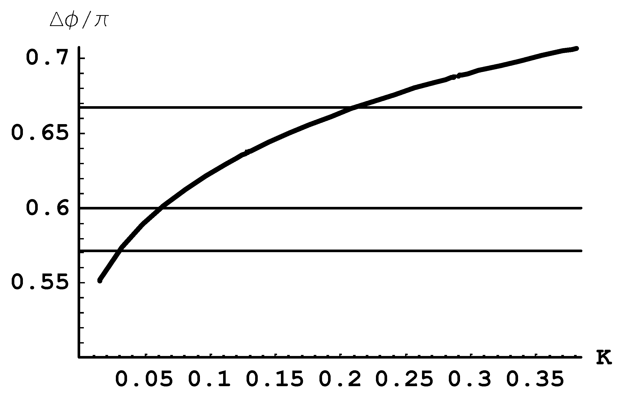
the trajectory becomes a close curve and the motion becomes periodic. Below we present three examples corresponding to the three lowest pairs of integers n and m in Equation (34): (n = 2, m = 3), (n = 3, m = 5), and (n = 4, m = 7). Figure 9 illustrates where (i.e., at which values of K) the curve Δφ(K)/π intersects n/m for the above three pairs.
Δφ(K) = nπ/m,
Here are the details for all three cases. In the case of n = 2, m = 3, during three periods of the θ-oscillations, the angle φ completes two full circles. This happens for K = 0.2103.
In the case of n = 3, m = 5, during five periods of the θ-oscillations, the angle φ completes three full circles. This happens for K = 0.0632.
In the case of n = 4, m = 7, during seven periods of the θ-oscillations, the angle φ completes four full circles. This happens for K = 0.0310.
These examples show, in particular, that the θ-oscillations can actually occur on the same time scale as the φ-precessions. The same is true in the general case of the conditionally-periodic orbits of the electron. Thus, the statement from work [8] that “in general the motion should consist of large oscillations with respect to the polar angle θ combined with a slow precession about the z-axis” is incorrect.
3. Conclusions
We considered the classical bound motion of a Rydberg electron around a polar molecule. We showed that in the general case, where the motion consists of the oscillations in the upper hemisphere in the meridional direction (θ-direction) combined with the precession along parallels of latitude (φ-direction), both the θ-oscillations and the φ-precessions can actually occur on the same time scale, so that the statement to the contrary from work [8] is incorrect. (We also corrected one of the equations in paper [6].)
We obtained the relation between the two dynamical variables, i.e., the dependence of φ on θ in the form of a one-fold integral in the general case and illustrated it pictorially. We also derived an explicit analytical result for φ(θ) in the case where the dimensionless parameter K = pφ2/(2meD) << 1, i.e., for relatively small values of the projection pφ of the angular momentum on the axis of the electric dipole.
For the particular case of K = 0, where the electron oscillates along a semicircle crossing the north pole, we derived an explicit analytical result for the dependence of time t on θ. For the opposite particular case, where K = Kmax = 2/33/2 and the electron follows a circular path along the parallel of latitude corresponding to θ = 0.9553 rad = 54.74 degrees, we obtained an explicit analytical result for the period of the revolution.
Further, we obtained the time evolution of the dynamical variable θ and the period Tθ of the θ-oscillations in the form of a one-fold integral in the general case and illustrated it pictorially. We also derived the corresponding explicit analytical expressions for the case of K << 1.
We also obtained the change of the angular variable φ during one half-period of the θ-motion in the form of a one-fold integral in the general case. We provided a pictorial illustration of this result.
Finally, we studied whether there are values of the parameter K, such that this conditionally-periodic motion would become truly periodic, so that the trajectory of the electron would become a closed curve. We derived a general condition for this to happen and then provided three examples of the values of K, enabling the motion to become periodic.
We believe that our classical results provide a physical insight into the complicated dynamics of a Rydberg electron around a polar molecule.
Funding
This research received no external funding.
Conflicts of Interest
The author declares no conflict of interest.
References
- Fermi, E.; Teller, E. The capture of negative mesotrons in matter. Phys. Rev. 1947, 72, 399–408. [Google Scholar] [CrossRef]
- Connolly, K.; Griffiths, D.J. Critical dipoles in one, two, and three dimensions. Am. J. Phys. 2007, 75, 524–531. [Google Scholar] [CrossRef]
- Turner, J.E.; Fox, K. Classical motion of an electron in an electric-dipole field. I. Finite dipole case. J. Phys. A 1968, 1, 118–123. [Google Scholar] [CrossRef]
- Kryukov, N.; Oks, E. Muonic–electronic negative hydrogen ion: Circular states. Can. J. Phys. 2013, 91, 715–721. [Google Scholar] [CrossRef]
- Kryukov, N.; Oks, E. Super-generalized Runge-Lenz vector in the problem of two Coulomb or Newton centers. Phys. Rev. A 2012, 85, 054503. [Google Scholar] [CrossRef]
- Fox, K. Classical motion of an electron in an electric-dipole field. II. Point dipole case. J. Phys. A (Proc. Phys. Soc.) 1968, 1, 124–127. [Google Scholar] [CrossRef]
- Jones, R.S. Circular motion of a charged particle in an electric dipole field. Am. J. Phys. 1995, 63, 1042–1043. [Google Scholar] [CrossRef]
- McDonald, K.T. Motion of a Point Charge near an Electric Dipole. 1996. Available online: http://www.hep.princeton.edu/~mcdonald/examples/dipole.pdf (accessed on 1 July 2020).
Figure 1.
Three-dimensional plot of the polynomial y(x, K) from Equation (6).

Figure 2.
Plot of both positive roots x2 and x3 of the cubic Equation (8) versus K = pφ2/(2meD).

Figure 3.
Dependence of the scaled time τ (defined in Equation (12)) on x = cosθ during one half-period of the electron oscillation along a semicircular path through the north pole of the upper hemisphere (K = 0).
Figure 3.
Dependence of the scaled time τ (defined in Equation (12)) on x = cosθ during one half-period of the electron oscillation along a semicircular path through the north pole of the upper hemisphere (K = 0).

Figure 4.
Evolution of the scaled time τ during one period of the θ-motion for K = 0.1 (solid line), K = 0.2 (dashed line), and K = 0.3 (dotted line).
Figure 4.
Evolution of the scaled time τ during one period of the θ-motion for K = 0.1 (solid line), K = 0.2 (dashed line), and K = 0.3 (dotted line).

Figure 5.
Comparison of the approximate analytical result for τ(x, K) from Equation (23) for K = 0.01 (solid line) with the corresponding exact result obtained by the numerical integration in Equation (22) (dashed line).
Figure 5.
Comparison of the approximate analytical result for τ(x, K) from Equation (23) for K = 0.01 (solid line) with the corresponding exact result obtained by the numerical integration in Equation (22) (dashed line).

Figure 6.
Dependence of the scaled period Tθ of the θ-motion on the parameter K = pφ2/(2meD). The period Tθ is in units of mr4/(2eD).
Figure 6.
Dependence of the scaled period Tθ of the θ-motion on the parameter K = pφ2/(2meD). The period Tθ is in units of mr4/(2eD).

Figure 7.
Dependence of φ on x = cosθ during one half-period of the θ-motion for K = 0.1 (solid line), K = 0.2 (dashed line), and K = 0.3 (dotted line).
Figure 7.
Dependence of φ on x = cosθ during one half-period of the θ-motion for K = 0.1 (solid line), K = 0.2 (dashed line), and K = 0.3 (dotted line).

Figure 8.
Comparison of the approximate analytical result for φ(K, x) from Equation (30) for K = 0.02 (solid line) with the corresponding exact result from Equation (29) (dashed line).
Figure 8.
Comparison of the approximate analytical result for φ(K, x) from Equation (30) for K = 0.02 (solid line) with the corresponding exact result from Equation (29) (dashed line).

Figure 9.
Intersections of the curve Δφ(K)/π (thick line) with the tree horizontal lines corresponding to 2/3 (the top thin line), 3/5 (the middle thin line), and 4/7 (the bottom thin line). For the values of K, corresponding to these intersections, the motion, which is generally conditionally-periodic, becomes truly periodic.

© 2020 by the author. Licensee MDPI, Basel, Switzerland. This article is an open access article distributed under the terms and conditions of the Creative Commons Attribution (CC BY) license (http://creativecommons.org/licenses/by/4.0/).
Share and Cite
MDPI and ACS Style
Oks, E. Oscillatory-Precessional Motion of a Rydberg Electron Around a Polar Molecule. Symmetry 2020, 12, 1275. https://doi.org/10.3390/sym12081275
AMA Style
Oks E. Oscillatory-Precessional Motion of a Rydberg Electron Around a Polar Molecule. Symmetry. 2020; 12(8):1275. https://doi.org/10.3390/sym12081275
Chicago/Turabian StyleOks, Eugene. 2020. "Oscillatory-Precessional Motion of a Rydberg Electron Around a Polar Molecule" Symmetry 12, no. 8: 1275. https://doi.org/10.3390/sym12081275
Note that from the first issue of 2016, this journal uses article numbers instead of page numbers. See further details here.