Bi-Directional Filter for the Removal of Lines and Cracks in Images


Faculty of Engineering and Information Technology, Al-Azhar University, Gaza 79715, Palestine
Symmetry 2020, 12(8), 1280; https://doi.org/10.3390/sym12081280
Submission received: 30 June 2020
/
Revised: 28 July 2020
/
Accepted: 29 July 2020
/
Published: 2 August 2020
(This article belongs to the Special Issue Symmetry in Engineering Sciences Ⅲ)
Abstract
:In this paper, a method for the removal of noisy lines and cracks corrupted by different noise types is explored, using a cascade of filtering cycles based on the principle of symmetry among neighboring pixels. Each filtering cycle includes a filter in two perpendicular directions, one horizontal and the other vertical. Any pixel, to be deemed original, should have a number of symmetric pixels within its neighboring pixels greater than the number specified by the condition set for each direction in all the filters. Since the conditions of each filter increase gradually from one cycle to the next, it becomes more difficult for a noisy pixel to satisfy the filter conditions in each filtering cycle, while an original pixel can easily satisfy the conditions in all the filtering cycles. The reason is that a noisy pixel has a random value and therefore faces difficulty in finding a sufficient number of symmetric pixels in each direction, while an original one has a value correlated with the values of its neighboring pixels. Extensive simulation experiments prove that the proposed method efficiently detects and restores different noisy lines and cracks of different shape and thickness. Also, it retains the image details and outperforms other well-known algorithms, both objectively and subjectively. More specifically, the proposed algorithm achieves restoration performance better than the other known methods by ≥0.81dB in all simulation experiments.

1. Introduction
Image denoising is one of the important processes that should be implemented before any advanced image processing method. The reason is that any advanced method will deliver unsatisfactory results if it is implemented on images contaminated with low or high rates of noise. As an example, you cannot exclusively select or detect edge pixels from noisy images. Thus, many algorithms are proposed in the literature to remove noise from images corrupted by salt-and-pepper noise, random-valued impulse noise, Gaussian noise, a mixture of two or more of them, or other types of noise. All the proposed methods utilize the prior information in the corrupted images to remove the noise in the corrupted images at a specific level. Various approaches are implemented for Gaussian noise removal, such as the bi-linear filter, [1] which utilizes internal prior information obtained due to the similarity attributes among the pixels in the local region to restore a corrupted pixel. Many others are applied for Gaussian noise removal that utilize internal prior information available among the pixels in non-local regions, such as the NLM algorithm [2,3]. External prior information may be extracted from other original images [4,5,6,7]. Other methods utilize internal prior information available in the corrupted images and external prior information available in the external clean images, such as those described in [8,9,10,11]. The authors in [12] map external prior information onto the corrupted image to generate a restored image. The advantage of this method is that it can be applied on a few training samples. One of the most effective methods in the literature used in the removal of Gaussian noise is Sparse 3-D Transform-Domain Collaborative Filtering, BM3D [13], in which a 3-D array is constructed from a group of similar blocks, then a 3-D transform is implemented on the 3-D array. The result is a highly sparse representation of the true signal, which helps in separating the noise by a shrinkage process. In [14], a new method for Gaussian noise removal is proposed through the development of the Blind Universal Image Fusion Denoiser, BUIFD, in which an optimal fusion denoising function is derived and integrated in a deep-learning architecture. For removing Gaussian noise, Izadi et al. [15] use external prior information, which is the mutual information from the spatial and temporal noise statistics, while Dong et al. [16] use the internal prior information attained from image nonlocal redundancy to better estimate the sparse coding coefficients of the original image.
Another type of noise that may degrade the image in real life is random-valued impulse noise, which is difficult to detect because it may take any value from the same range as the image pixels. In other words, random-valued impulse noise may take any value in the range from 0 to 255. For removal of random-valued impulse noise, many methods have been proposed to provide satisfactory results, as described in [17,18,19,20]. In [21], Chen et al. proposed the Tri State Median Filter, TSMF, which is a well-known method used for the removal of random-valued impulse noise, in which a threshold T is applied on the output of a center weight median filter and standard median filter, and as a result three possible state outputs are obtained. Namely, the pixel is original, noisy, or uncorrupted, with center weight wc > 1. In [22], Chen and Wu proposed the Adaptive Center Weight Median Filter, ACWMF, in which the differences between the current pixel in the sliding window and the outputs of center-weighted median filters are used for removing random-valued impulse noise. In [23], Crnojevic et al. proposed iterative Pixel-Wise modification of the Median of the Absolute Deviations from the median, PWMAD, for detecting random-valued impulse noise.
The third type of noise is salt-and-pepper impulse noise, which may take on two possible values, 0 (salt) and 255 (pepper). In recent years, many methods have been proposed for the removal of salt-and-pepper noise, for example those in [24,25]. In [26], Erkan et al. proposed the Adaptive Frequency Median Filter (AFMF), in which a median frequency function is used to restore the noisy pixels. The Noise Adaptive Fuzzy Switching Median Filter, NAFSMF [27], is another well-known method used for the removal of salt-and-pepper noise. It is a two-stage method. In the first stage, a histogram of the corrupted image is used for noise detection, and in the second stage fuzzy reasoning is used for restoration of the noisy pixels. The Adaptive Weighted Mean Filter, AWMF, proposed in [28], involves a sliding window which is gradually increased, and a tested pixel is considered as a noise candidate if it is equal to the detected maximum or minimum value. Image denoising methods based on deep learning have experienced rapid development. The Convolutional Neural Network, CNN [29,30,31], provides adequate denoising performance and can adaptively accomplish noise reduction in corrupted images. A new method, the Deep Convolutional Neural Network, DNCNN [32], has been proposed to obtain higher peak signal-to-noise ratio values than conventional methods. The Super-Resolution Convolutional Neural Network, SRCNN [33,34], model has been advanced for reconstructing images with more texture and detailed information. In [35], Xiu and Su proposed a new Composite Denoising Network, CDN, based on both an auto encoder to perform image denoising and a super-resolution reconstruction model to recover the texture and detailed information in the denoised image. In [36], Kunaraj et al. proposed a Machine Learning, ML, based classification algorithm which uses random decision forest classifiers and classical pixel-wise statistical parameters for better denoising of images corrupted by impulse noise. A hybrid filter which is an integration of the median filter and applied median is described in [37]. It mainly emphasizes the discarding of irrelevant noise.
One can observe that all of the previous methods depend mainly on internal prior information extracted from the pixels in the corrupted images, or they may use other external prior information to build a model or a filter for the removal of some specific types of noise. Thus, some of these methods face difficulties in obtaining enough prior information if different noise types contaminate the image or if the noise occurs in lines, cracks, or any other shape, and therefore corrupt a complete part or parts in the image. To address these shortcomings, a new method is proposed in this paper to detect and restore different types of noise, and to detect and restore lines and cracks that include only noisy pixels.
In this paper, an efficient method is proposed to remove noisy lines and cracks in images. All the pixels in the cracks and lines may be Gaussian noise, random-valued impulse noise, or salt-and-pepper impulse noise, or may be others. In the current study, it is assumed that there are two types of pixels in the image. The first type is noisy pixels, which form the noisy lines or cracks, and the other type is noise-free pixels, which represent the original parts of the image. Let x denote any pixel in the noisy lines or cracks in the corrupted image. The value of x represents one of the different types of noise in the dynamic range [a, b]. If x represents salt and pepper noise (SPN), then in this case a = 0 and b = 255, and x may be equal to 0 or 255 (equally likely). If x represents random-valued impulse noise (RVIN), then x is uniformly distributed and may take any value in the range [0,255]. If x represents Gaussian noise (GN), then x is normally distributed with mean m and standard deviation σ as:
where the symbol is used herein to denote the word distributed. Note that the range [a,b] in RVIN may be changed if one would like to generate values within specific limits, as in white and black lines. In other words, since the cracks usually have black or white color similar to the image background, or some shade of gray, values equal to a and b or the range between them should be selected to represent the color of the cracks or other lines corrupting some parts of the image.
The goal of this study is to detect and restore all the noisy pixels in the lines and cracks and at the same time leave the original values intact. It is clear that a horizontal crack or line has limited width in the vertical direction and significant length in the horizontal direction, and vice versa. Therefore, the noisy pixels may have enough similar pixels among their neighboring pixels in one direction but not in the other. As an example, each pixel in a vertical line at any particular point has some number of similar pixels in the horizontal direction, but an additional number of similar pixels in the vertical direction. However, it is difficult for a noisy pixel, in a line or crack of any direction, to have enough similar pixels in both directions to fulfill the similarity conditions. Therefore, they can be detected easily. Also, it is notable that the width or length of any line or crack is variable. Accordingly, we need a multi-cycle filter to handle different lengths and widths to efficiently detect the noisy pixels. To this end, the suggested algorithm consists of a cascade of filtering cycles, each of which includes a bi- directional filter. One of the directions is horizontal and the other is vertical, and each has a detection threshold. Any tested pixel is deemed original if it satisfies the set condition in each of the two directions of the proposed filter in all the filtering cycles. If the tested pixel fails to satisfy the conditions in any filtering cycle, it is considered a noisy pixel. Specifically, the pixel is deemed original in any cycle k if it has symmetric pixels with probability not less than the threshold probability in both directions. A pixel that does not satisfy the condition in any direction of any cycle is considered a noisy pixel and restored at the end of the filtering cycle. The noise from the image is removed gradually, in the sense that each filtering cycle is responsible for removing a specific amount of noise, because in each filtering cycle few of the pixels satisfy both conditions or have enough symmetric pixels in both directions.
One can expect that the pixels in thick lines or cracks may satisfy the conditions of both the horizontal and vertical directions in one or more filtering cycles. Consequently, as the thickness increases, more filtering cycles are needed to detect the noise. It should be noted that if the thickness of the noisy lines or cracks is increased to a certain degree, then after a specific number of filtering cycles, some of the image details may be lost. The reason is that the set conditions in the advanced cycles become difficult for the original pixels to satisfy, and as a result they will be considered noisy pixels. Thus, for noisy cracks or lines at a certain degree of thickness, removing the noise and keeping image details is a challenge.
2. Algorithm Description
The structure of the proposed filter is described in Figure 1. As shown in the figure, the filter consists of several cycles. In each cycle k there is a filter in two directions; one is vertical, which represents the height of the filter, and the other is horizontal, which represents the width of the filter, and both of the filter directions are involved in detecting the noisy pixels. The length of the filter in each cycle is measured in terms of the number of pixels in each direction. As an example, in the first cycle the filter length is five pixels, i.e., L1 = 5. That means that the height of the filter is five pixels and the width is five pixels, all centered at the tested pixel. The tested pixel is considered original if it has a number of similar or symmetric pixels among its four neighboring pixels, with probability not less than the threshold probability in each direction. The noisy pixels may fulfill the threshold probability in each direction in one or more cycles, but they cannot fulfill the set threshold probabilities in all the filtering cycles. The reason is that the noisy pixels take on random values, but the original pixels usually take values similar to those of their neighboring pixels. The proposed algorithm is described and formulated as follows.
1- We assume that any tested pixel x is symmetric to pixel y if the intensity difference between them is less than or equal to an accepted range of error, bounded from zero to ε, where ε is an integer representing the intensity difference between the two symmetric pixels as follows:
2- Each tested pixel x(i,j) in location i,j will pass through each cycle k, 1 ≤ k ≤ K, with K an integer, to be considered as an original pixel. In each cycle there is a filter in two directions, one vertical (Dv) and the other horizontal (Dh), each of length Lk pixels. For example, for an odd number Lk, the horizontal and vertical directions around the tested pixel x(i,j) will include the following pixels. Let a number N = (Lk − 1)/2, then Dh and Dv in the current cycle k will be expressed as:
As an example, for L1 = 5 and i = j = 0, then N = 2, = [ x(0,−2) x(0,−1) x(0,1) x(0,2)] and = [ x(−2,0) x(−1,0) x(1,0) x(2,0)]
3- In each filtering cycle k, a searching process is performed among the pixels in the vertical and horizontal directions to find any pixel y that is symmetric to the tested pixel x. Then, pixel y is saved in a set S as:
4- The probability of the tested pixel x in each direction at the current cycle k is calculated as:
is the number of the pixels y in the set S in the current direction at cycle k.
5- If the probability of the tested pixel x in the horizontal direction and the probability of x in the vertical direction are less than the threshold probability , then the tested pixel is considered noisy; otherwise, it is considered original, as:
x = xnoisy otherwise x = xoriginal.
6- if x is considered an original pixel in the current filtering cycle, it will pass to the next cycle to be tested in the second cycle. Any pixel that satisfies the threshold probability in all the filtering cycles is considered original. The suggested threshold probability and the filter length of each direction in the proposed algorithm is defined as and Lk = 3 + 2k for k = 1,2,3…K. As an example, the threshold probability in the first cycle will be . The number of cycles increases as the thickness of the noisy line or crack increases. The reason is that the noisy pixels in the thick line or crack can satisfy the threshold probabilities of the first few cycles, but they face difficulties in fulfilling the robust threshold probabilities of the last cycles.
7- At the end of each cycle, we restore the noisy pixels, and the quality of each output is objectively and subjectively evaluated to measure the strength of the proposed filter. In other words, the similarity between the restored pixels and the original pixels is measured in terms of peak signal-to-noise ratio, which approaches infinity as the Mean Square Error (MSE) between the intensity values of the original and restored versions approaches zero. Therefore, as the value of peak signal-to-noise ratio increases, the restored version becomes more similar to the original version and vice versa. Also, sometimes we may find that restored versions provide somewhat high peak signal-to-noise ratio values, but still contain residual noise. Accordingly, human visual perception as a subjective evaluation is essential. Therefore, image visual appearance should be evaluated based on human perception after each filtering cycle, which in turns consumes extra computational time. Also, a structural similarity parameter is used as well for evaluating the visual quality of the restored versions.
The restoration process is achieved by taking the median of the nearest 4, 8, or more pixels around the noisy pixel. If four neighboring pixels are considered, then the restoration process for is defined as:
The pixels in the vector Z are either original or previously restored pixels, and the number of the pixels in the vector Z increases as the thickness of the noisy line or crack increases or the number of the detected noisy pixels increases.
The block diagram shown below in Figure 2 describes the steps from 3–9 mentioned above in the current section. Note that the first cycle filters the noisy image. Then, if the restored image shows an acceptable visual quality, the algorithm is terminated; otherwise, the algorithm moves to the next cycle, in which the pixels that were detected as original in the previous filter are tested another time. At the end of second cycle, the noisy pixels are restored, and if the restored version has no residual noise and shows a pleasing appearance, then the algorithm is terminated. Otherwise, the algorithm is moved to the third cycle and so on. The algorithm may be run for several cycles and the user may select the version with the best visual quality among all the restored versions.
3. Simulation Results
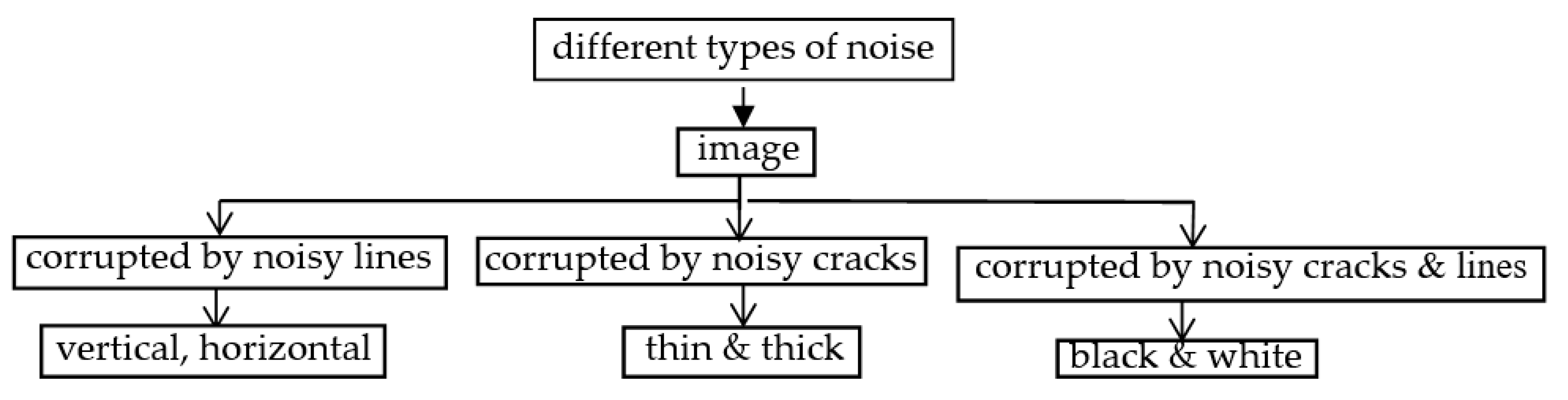
In this section, we evaluate the proposed algorithm objectively in terms of peak signal-to-noise ratio (PSNR) and Structural Similarity (SSIM) index, and subjectively in terms of human perception. To this end, different simulation experiments are implemented on different image structures to show the strength of the proposed method in removing the noisy lines and cracks in images. Noisy pixels in the lines or cracks may pass through one or more filtering cycles depending on the thickness of the lines or cracks, but they face difficulties in passing through all the filtering cycles of the proposed algorithm. The results of the proposed method are compared with other well-known methods used in the image denoising field, such as B3DM [13], TSMF [21], ACWMF [22], PWMAD [23], NAFSM [27], and AWMF [28]. One more advantage of the proposed technique is that the results are attained by tuning only one parameter, which is the accepted range of error ε, but the others remain intact. The original image is corrupted artificially with horizontal lines, vertical lines, and cracks all of different thickness. All the pixels in the lines or cracks are noisy pixels, which means that the lines and cracks are completely corrupted. The values of the noisy pixels in the range between [a, b] are generated to represent the color of the cracks and lines produced in the image due to environmental or any other external effects on the image. The color of the cracks and the lines may either be white or black, similar to the image background, or various gray-scale levels. For white lines, the values of a and b are very high and close to 255, for example a = 200 and b = 250, and the range [a, b] = [200, 255]. For black lines, the values of a and b are close to zero, for example a = 0 and b = 20. For lines corrupted with RVIN, a = 0 and b = 255 and the noisy pixel may take on any value in the range between 0 and 255. For lines corrupted with SPN, the noise takes values of either 0 or 255 with equal probability. In the simulation experiments, all the above noisy values, which represent RVIN, SPN, or any other range, are uniformly distributed and generated using the MATLAB rand function. For gray-level noise, the values of the noisy pixels are generated from a uniform or Gaussian distribution in the range between 0 and 255. Gaussian noise is characterized by the mean m and standard deviation σ, and can be generated using the MATLAB randn function. Cracks are created randomly on the original images using the pen in the Microsoft Paint program. In all the filtering cycles, the length Lk and the probability condition of each filter at cycle k are equal to Lk = 3 + 2k, k = 1, 2, 3…K, and , respectively. Figure 3 shows a summary of the types of the experiments implemented in this study to demonstrate the effectiveness of the proposed method. It is notable that different images corrupted by noisy lines, noisy cracks, or a combination are used in the simulation experiments. In addition, noisy lines and cracks containing different types of noise and of different thickness, shapes, and colors are restored efficiently by the proposed method.
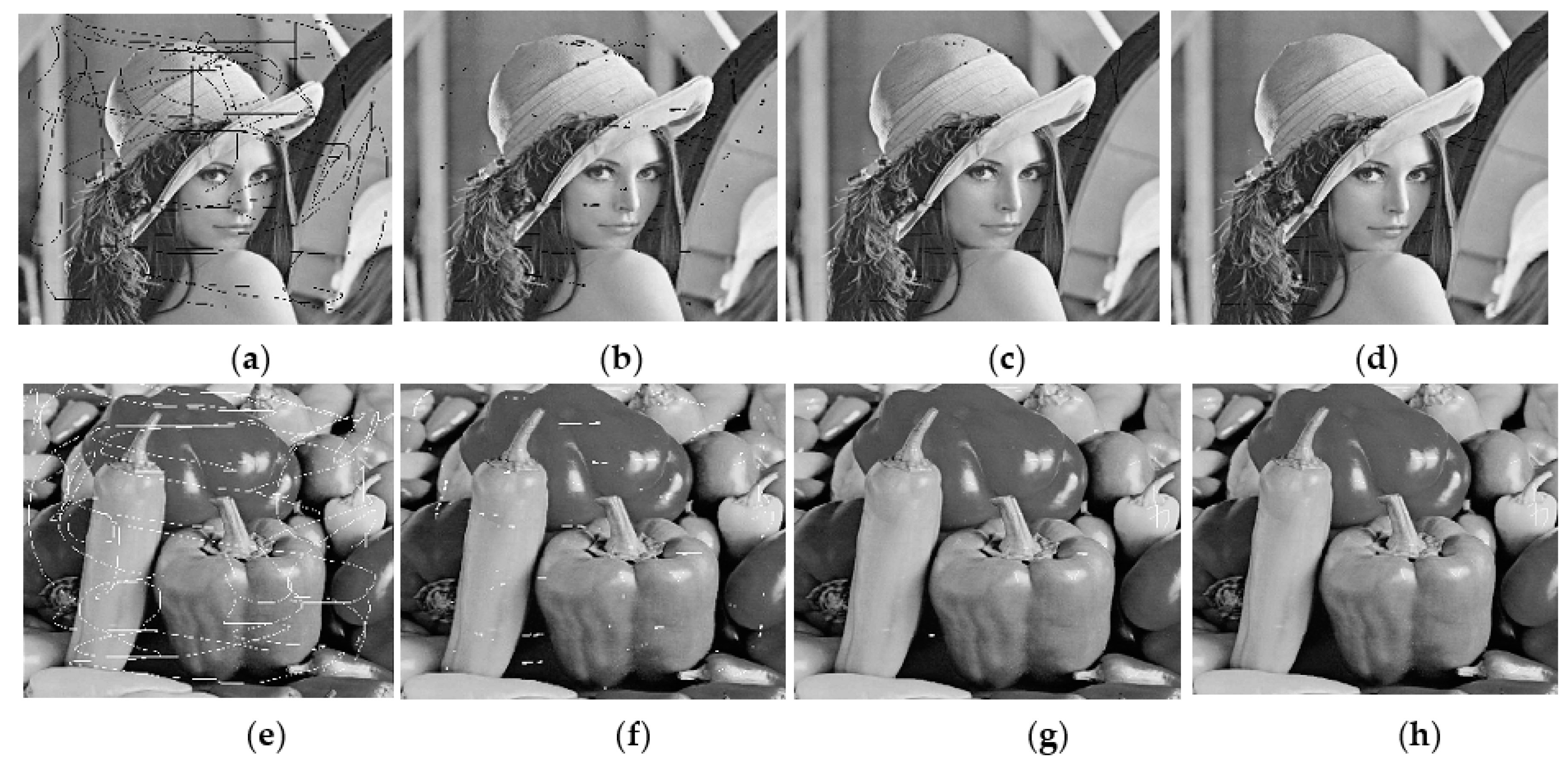
Figure 4 shows the output after each filtering cycle in restoring two corrupted versions, one for a Lena image and the other for a Pepper image at accepted range of error ε = 45. The corrupted version of the Lena image includes black lines and cracks, while the corrupted version of the Pepper image includes white lines and cracks. It is clear that the noise is removed through three filtering cycles, where each filtering cycle removes a specific amount of noise in the sense that a pixel that does not satisfy the condition in each cycle is considered noisy and restored after each cycle. In this experiment, the number of filtering cycles is k = 3, which means that the restored version attained from the third filtering cycle is visually pleasing. Figure 5 illustrates the restoration performance of different methods in restoring the cracks in the corrupted Lena image shown in Figure 4. It is clear that the proposed method delivers the best results, either in terms of PSNR in dB or visual quality of the image. Three phases are sufficient to eliminate the noisy cracks or lines from the corrupted image in this experiment with ε = 45.
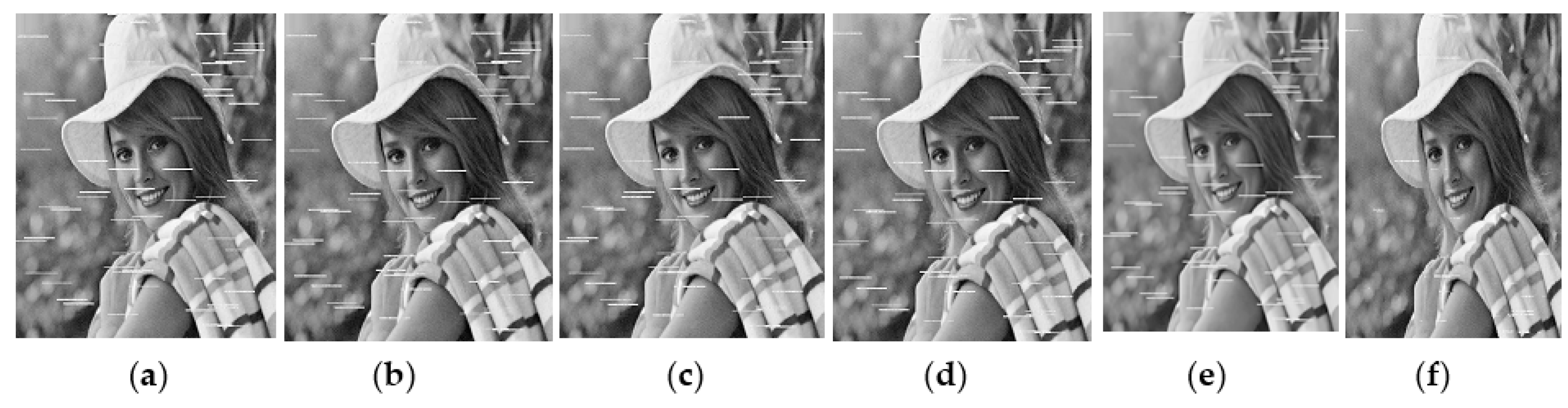
In Figure 6, Elaine image corrupted with 60 white lines is used to evaluate the performance of different methods. It is clear that the proposed method has the best performance, while the others still have almost the same amounts of noisy pixels after processing. Note that the accepted range of error used in this figure is equal to ε = 45 and number of cycles is equal to k = 4.
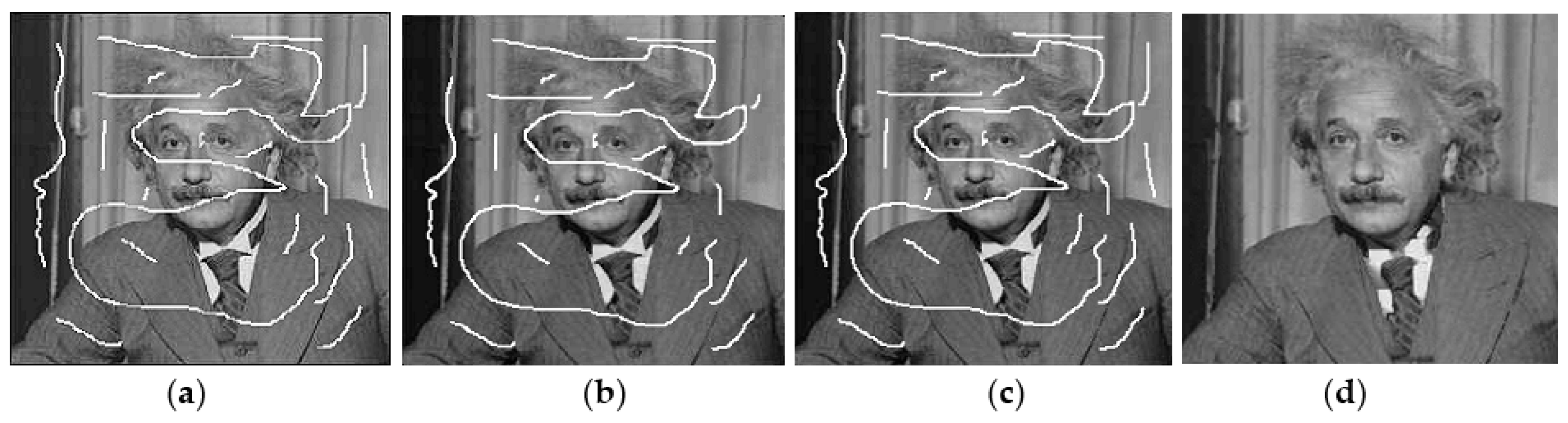
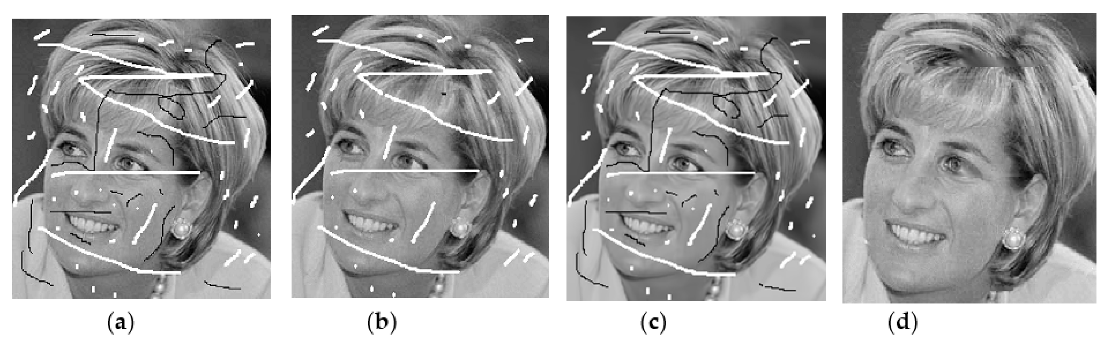
Figure 7 and Figure 8 show the restoration performance of different methods in restoring cracks that are much thicker than the ones appearing in the corrupted images mentioned in Figure 3. Also, Figure 8 includes black cracks in addition to white ones. It is clear that the proposed method still outperforms the other well-known methods.
Also, it is recommended that one increase the number of cycles and the accepted range of error as the thickness of the lines or cracks increases. Therefore, the acceptable range of error used in both figures is equal to ε = 66. The number of cycles is equal to k = 3 in Figure 7 and k = 8 in Figure 8.
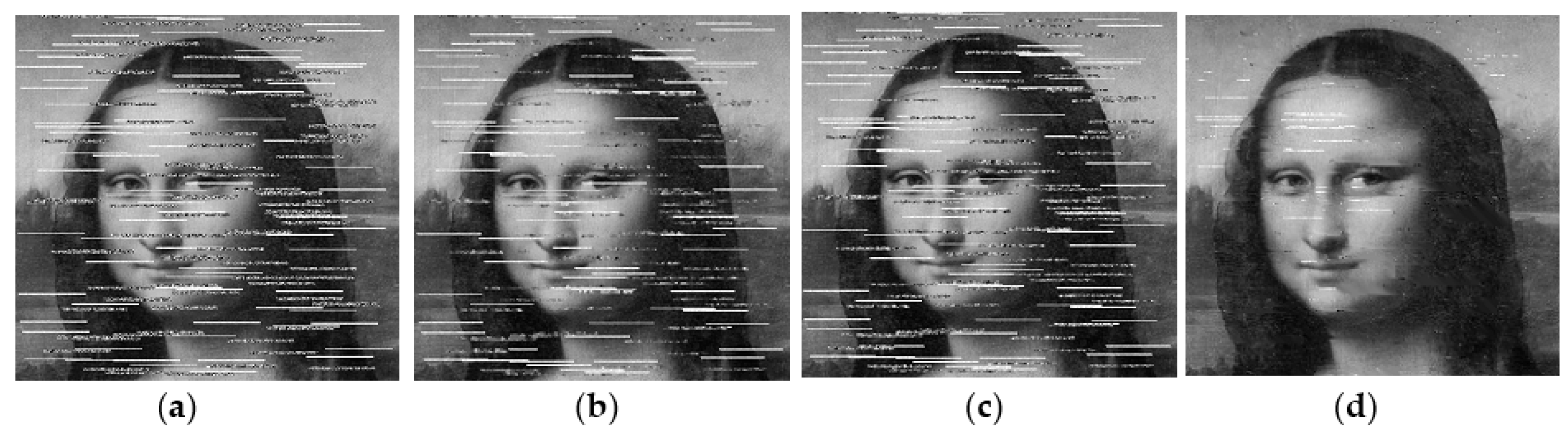
In Figure 9, 80 white lines and 80 gray-level lines corrupt the Mona Lisa image. Gray-level lines may take any value in the range of [0,255] at equal probability. It can be seen that the proposed method removes 160 lines from the corrupted image effectively either in terms of PSNR or human visual quality, while the other methods fail to restore this kind of highly corrupted image. In this experiment, the number of phases is k = 5 and the accepted range of error is ε = 60.
Figure 10 shows the outputs of three cycles in the proposed algorithm at acceptance range of error ε = 60, to illustrate the process of gradual restoration by the proposed algorithm. Besides, the results of the proposed algorithm are compared in this figure with the results of other methods. The input to the proposed filter in this experiment is a tulip flower image corrupted with 80 vertical lines of noisy values generated from a normal distribution with mean 200 and standard deviation σ = 1. It is apparent that the 5th filtering cycle fails to remove the residual lines in the image, but they are removed after the 6th filtering cycle at the expense of PSNR. Also, it is clear that the proposed method delivers the best restoration performance in terms of visual quality and PSNR. A small amount of residual noise may appear in the restored images attained from highly corrupted images, as in Figure 9, or from images corrupted by thick lines or cracks, as in Figure 8. Thus, one may use a simple thresholding method or any other method to remove any residual noise rather than using a new cycle.
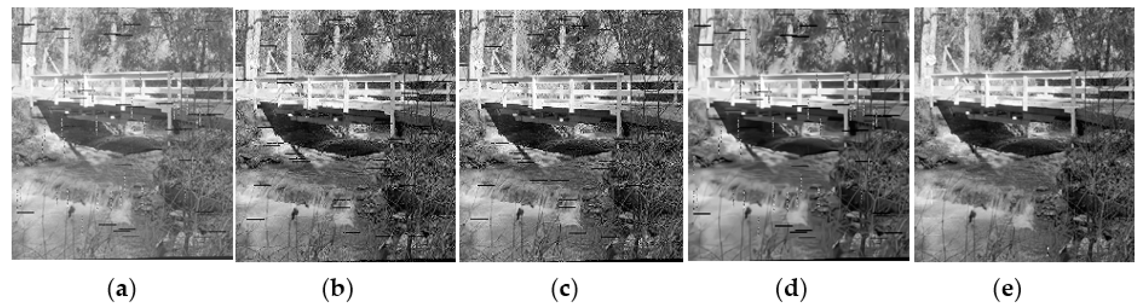
Figure 11 shows the performance for the different methods in restoring a Bridge image corrupted by 40 vertical lines and 40 horizontal lines. The noisy values of the vertical lines are salt-and-pepper noise, while the noisy values of the horizontal lines are Gaussian noise of mean zero and standard deviation σ = 20. It is clear that the methods in (b) and (c) effectively restore the vertical lines, but they fail to remove the horizontal lines because they mainly detect and restore only two values, salt = 255 and pepper = 0. BM3D fails even to restore the Gaussian noise in the horizontal lines; the reason is that the entire pixels in the lines and cracks have been replaced completely by Gaussian noise.
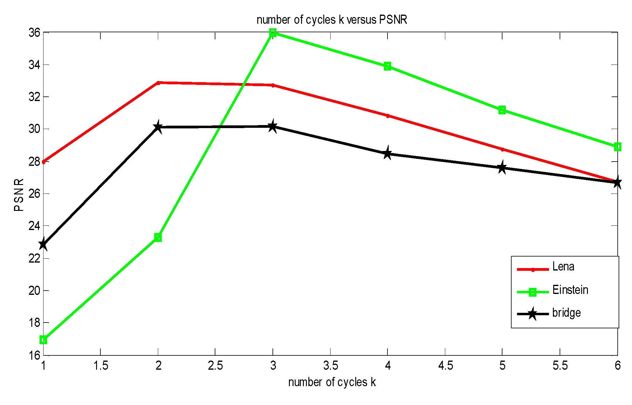
Therefore, there is not enough information on the original values. Also, it is obvious that the proposed method in (e) effectively restores both the vertical and the horizontal lines. Figure 12 shows the PSNR values of different restored versions attained after each filtering cycle in the proposed method. Three images are used in this experiment. The first one is the corrupted version of the Lena image mentioned in Figure 5, the second one is the corrupted version of the Einstein image mentioned in Figure 7, the last one is the corrupted version of the Bridge image mentioned in Figure 11. Six restored versions are attained for each image after each filtering cycle. It is clear that for each image there is at least one filtering cycle after which the result is acceptable. Figure 13 shows the effect of the accepted range of error ε on the restored versions attained after each filtering cycle in the proposed method. The corrupted Einstein image mentioned in Figure 7 is used in this experiment. It is clear that as the value of ε increases, the PSNR increases, but to a specific value. In other words, if ε is increased more and more to ε = 100, then a poor result is provided. The reason is that as ε increases, many noisy pixels will be similar to each other and satisfy the set conditions in each filtering cycle.
Table 1 and Table 2 show the restoration performance in terms of PSNR and SSIM, as well as the consumed time in seconds, for different methods in restoring the corrupted versions mentioned in Figure 11 for the Bridge image and Figure 7 for the Einstein image, respectively. Note that the size of the Einstein image is 256 × 256 and the size of the Bridge image is 512 × 512. These results are implemented in MATLAB on a computer with an HP ENVY TS 14 Sleekbook Intel Core [email protected] CPU. It is obvious that the proposed method objectively delivers the best results, besides providing computational complexity lower than other methods. In other words, one can conclude that the proposed method is very efficient and easy to implement, since the process in each filtering cycle involves simple mathematical equations. The strength of the proposed method is that whatever the structure of the image, any pixel that does not achieve the minimum requirements in each cycle is considered a noisy pixel. The minimum requirements in each cycle can be achieved easily by each original pixel in the image due to the redundancy of the original pixels in the local regions, but in most cases a noisy pixel does not have sufficient redundant pixels. However, the proposed algorithm provides good results for noisy lines and cracks to a certain degree of thickness. In recent years, deep-learning-based methods have achieved remarkable success in a number of research areas, such as image and voice recognition. Therefore, one can take advantage of deep learning in order to enhance the performance of the present study, particularly in restoring images corrupted with much thicker lines and cracks.
4. Conclusions
The current study explores the removal of noisy lines and cracks in images by using a cascade of cycles. Each cycle has a filter of two directions, one vertical and the other horizontal. Any pixel that satisfies the symmetric conditions in all the filtering cycles is considered original; otherwise, it is deemed noisy. A noisy pixel has a random value, and therefore it is difficult for any noisy pixel in a vertical or horizontal line or crack to satisfy the symmetry conditions in both directions in all the filtering cycles. As a result, the noisy pixels are detected gradually through the filtering cycles. The number of cycles should be increased as the thickness of the noisy lines or cracks is increased. All the simulated experiments implemented in this study indicate that the proposed algorithm delivers superior results compared to other well-known methods in preserving image details and removing different types of noise contaminating lines and cracks of different sizes. Since keeping image details while removing thicker lines or cracks is a challenge, this problem should be deeply investigated in future work.
Funding
This research received no external funding.
Conflicts of Interest
The author declares no conflict of interest.
References
- Tomasi, C.; Manduchi, R. Bilateral filtering for gray and color images. In Proceedings of the IEEE International Conference on Computer Vision (ICCV), Bombay, India, 7 January 1998; pp. 839–846. [Google Scholar]
- Buades, A.; Coll, B.; Morel, J.M. A non-local algorithm for image denoising. In Proceedings of the IEEE Conference on Computer Vision and Pattern Recognition (CVPR), San Diego, CA, USA, 20–25 June 2005; Volume 2, pp. 60–65. [Google Scholar]
- Lebrun, M.; Buades, A.; Morel, J.M. A nonlocal Bayesian image denoising algorithm. Siam J. Imaging Sci. 2013, 6, 1665–1688. [Google Scholar] [CrossRef]
- Zoran, D.; Weiss, Y. From learning models of natural image patches to whole image restoration. In Proceedings of the IEEE International Conference on Computer Vision (ICCV), Barcelona, Spain, 6–13 November 2011; pp. 479–486. [Google Scholar]
- Mosseri, I.; Zontak, M.; Irani, M. Combining the power of internal and external denoising. In Proceedings of the IEEE International Conference on Computer Vision, Cambridge, MA, USA, 19–21 April 2013; pp. 1–9. [Google Scholar]
- Chen, F.; Zhang, L.; Yu, H. External patch prior guided internal clustering for image denoising. In Proceedings of the IEEE International Conference on Computer Vision, Santiago, Chile, 7–13 December 2015; pp. 603–611. [Google Scholar]
- Luo, E.; Chan, S.H.; Nguyen, T.Q. Adaptive image denoising by targeted databases. IEEE Trans. Image Process. 2015, 24, 2167–2181. [Google Scholar] [CrossRef] [PubMed] [Green Version]
- Xie, J.; Xu, L.; Chen, E. Image denoising and inpainting with deep neural networks. Adv. Neural Inf. Process. Syst. 2012, 25, 341–349. [Google Scholar]
- Zhang, K.; Zuo, W.; Chen, Y.; Meng, D.; Zhang, L. Beyond a Gaussian denoiser: Residual learning of deep cnn for image denoising. IEEE Trans. Image Process. 2017, 26, 3142–3155. [Google Scholar] [CrossRef] [PubMed] [Green Version]
- Barbu, A. Training an active random field for real-time image denoising. IEEE Trans. Image Process. 2009, 18, 2451–2462. [Google Scholar] [CrossRef]
- Schmidt, U.; Roth, S. Shrinkage fields for effective image restoration. In Proceedings of the 2014 IEEE Conference on Computer Vision and Pattern Recognition, Columbus, OH, USA, 23 January 2014; pp. 2774–2781. [Google Scholar]
- Chan, S.; Luo, E.; Nguyen, T. Adaptive patch-based image denoising by EM-adaptation. In Proceedings of the IEEE Global Conference on Signal and Information Processing (GlobalSIP), Orlando, FL, USA, 14–16 December 2015. [Google Scholar]
- Dabov, K.; Foi, A.; Katkovnik, V.K.; Egiazarian, K. Image denoising by sparse 3-D transform-domain collaborative filtering. IEEE Trans. Image Process. 2007, 16, 2080–2095. [Google Scholar] [CrossRef]
- El, H.M.; Süsstrunk, S. Blind universal Bayesian image denoising with Gaussian noise level learning. IEEE Trans. Image Process. 2020, 29, 4885–4896. [Google Scholar]
- Izadi, M.; Birkbeck, N.; Balu, A.B. Mutual Noise Estimation Algorithm for Video Denoising. In Proceedings of the 2019 IEEE International Conference on Image Processing (ICIP), Taipei, Taiwan, 22–25 September 2019; pp. 2424–2428. [Google Scholar]
- Dong, W.; Zhang, L.; Shi, G.; Li, X. Nonlocally centralized sparse representation for image restoration. IEEE Trans. Image Process. 2013, 22, 1620–1630. [Google Scholar] [CrossRef] [Green Version]
- Roy, A.; Manam, L.; Laskar, R.H. Region adaptive fuzzy filter: An approach for removal of random-valued impulse noise. IEEE Trans. Ind. Electron. 2018, 65, 7268–7278. [Google Scholar] [CrossRef]
- Zhou, W.; Zhang, D. Progressive switching median filter for the removal of impulse noise from highly corrupted images. IEEE Trans. Circuits Syst. II Analog Digit. Signal Process 1999, 46, 78–80. [Google Scholar] [CrossRef] [Green Version]
- Dong, Y.; Xu, S. A new directional weighted median filter for removal of random-valued impulse noise. IEEE Signal Process. Lett. 2007, 14, 193–196. [Google Scholar] [CrossRef]
- Ko, S.-J.; Lee, Y.H. Center weighted median filters and their applications to image enhancement. IEEE Trans. Circuits Syst. 1991, 38, 984–993. [Google Scholar] [CrossRef]
- Chen, T.; Ma, K.; Chen, L. Tri-state median filter for image denoising. IEEE Trans. Image Process. 1999, 8, 1834–1838. [Google Scholar] [CrossRef] [PubMed] [Green Version]
- Chen, T.; Wu, H.R. Adaptive impulse detection using center-weighted median filters. IEEE Signal Process. Lett. 2001, 8, 1–3. [Google Scholar] [CrossRef]
- Crnojevic, V.; Senk, V.; Trpovski, Z. Advanced impulse detection based on pixel-wise MAD. IEEE Signal Process. Lett. 2004, 11, 589–592. [Google Scholar] [CrossRef]
- Fu, B.; Zhao, X.; Song, C.; Li, X.; Wang, X. A salt and pepper noise image denoising method based on the generative classification. Multimed. Tools Appl. 2019, 78, 12043–12053. [Google Scholar] [CrossRef] [Green Version]
- Fareed, S.B.S.; Khader, S.S. Fast adaptive and selective mean filter for the removal of high-density salt and pepper noise. IET Image Process. 2018, 12, 1378–1387. [Google Scholar] [CrossRef]
- Erkan, U.; Enginoğlu, S.; Thanh, D.N.H.; Hieu, L.M. Adaptive Frequency Median Filter for the salt- and pepper denoising problem. IET Image Process. 2019, 14, 1291–1302. [Google Scholar] [CrossRef]
- Toh, K.K.V.; Isa, N.A.M. Noise adaptive fuzzy switching median filter for salt-and-pepper noise reduction. IEEE Signal Process. Lett. 2010, 17, 281–284. [Google Scholar] [CrossRef] [Green Version]
- Zhang, P.; Fang, L. A new adaptive weighted mean filter for removing salt-and-pepper noise. IEEE Signal Process. Lett. 2014, 21, 1280–1283. [Google Scholar] [CrossRef]
- Li, J.; Li, G.; Fan, H. Image dehazing using residual-based deep CNN. IEEE Access 2018, 6, 26831–26842. [Google Scholar] [CrossRef]
- Min, C.; Wen, G.; Li, B.; Fan, F. Blind deblurring via a novel recursive deep CNN improved by wavelet transform. IEEE Access 2018, 6, 69242–69252. [Google Scholar] [CrossRef]
- Isogawa, K.; Ida, T.; Shiodera, T.; Takeguchi, T. Deep shrinkage convolutional neural network for adaptive noise reduction. IEEE Signal Process. Lett. 2018, 25, 224–228. [Google Scholar] [CrossRef]
- Yin, Z.; Wan, B.; Yuan, F.; Xia, X.; Shi, J. A deep normalization and convolutional neural network for image smoke detection. IEEE Access 2017, 5, 18429–18438. [Google Scholar] [CrossRef]
- Dong, C.; Chen, C.L.; Tang, X. Accelerating the super-resolution convolutional neural network. Eur. Conf. Comput. Vis. 2016, 9906, 391–407. [Google Scholar]
- Dong, C.; Loy, C.C.; He, K.; Tang, X. Image super-resolution using deep convolutional networks. IEEE Trans. Pattern Anal. Mach. Intell. 2016, 38, 295–307. [Google Scholar] [CrossRef] [Green Version]
- Xiu, C.; Su, X. Composite convolutional neural network for noise deduction. IEEE Access 2019, 7, 117814–117828. [Google Scholar] [CrossRef]
- Kunaraj, K.; Wenisch, S.M.; Balaji, S.; Bosco, F.M. Impulse Noise Classification Using Machine Learning Classifier and Robust Statistical Features. In Proceedings of the International Conference on Computational Vision and Bio Inspired Computing; Springer: Cham, Switzerland, 2020. [Google Scholar]
- Devakumari, D.; Punithavathi, V. Noise Removal in Breast Cancer Using Hybrid De-noising Filter for Mammogram Images. In Proceedings of the International Conference on Computational Vision and Bio Inspired Computing; Springer: Cham, Switzerland, 2020. [Google Scholar]
Figure 1.
The structure of the proposed filter: (a) A cascade of multiple filters, each having a bi-directional filter of different length Lk and probability condition . Each filter is implemented in a separate filtering cycle, (b) the 1st filter in the 1st cycle of L1 = 5 pixels in horizontal and vertical directions is applied to the original image, (c) the 2nd filter in the 2nd cycle of L1 = 7 pixels in the horizontal and vertical directions is applied on the pixels that are detected as original in the 1st cycle, and so on.

Figure 2.
Block diagram showing the cascading steps of the proposed algorithm.

Figure 3.
Summary of the types of the simulation experiments in this study.

Figure 4.
The output of each filtering cycle in the proposed algorithm for restoring the lines and cracks in noisy images: (a) Corrupted Lena image; (b) Output from 1st cycle, peak signal-to-noise ratio (PSNR) = 28; (c) Output from 2nd cycle, PSNR = 32.88; (d) Output from 3rd cycle, PSNR = 32.71; (e) Corrupted Pepper image; (f) Output from 1st cycle, PSNR = 28; (g) Output from 2nd cycle, PSNR = 34.86; (h) Output from 3rd cycle, PSNR = 33.84.

Figure 5.
Comparison between different methods in restoring the cracks in the corrupted Lena image shown in Figure 1: (a) Adaptive Center Weight Median Filter, ACWMF, PSNR = 31.9; (b) the Tri State Median Filter, TSMF, PSNR = 31.9; (c) Pixel-Wise modification of the Median of the Absolute Deviations from the median, PWMAD, PSNR = 27.3; (d) Sparse 3-D Transform-Domain Collaborative Filtering, BM3D, PSNR = 19.97; (e) proposed method, PSNR = 32.71.

Figure 6.
Comparison between different methods in restoring Elaine image corrupted by 60 white lines: (a) Corrupted image (b) ACWMF, PSNR = 25.2; (c) TSMF, PSNR = 23.19; (d) PWMAD, PSNR = 24.9; (e) BM3D, PSNR = 24; (f) proposed method, PSNR = 35.46.
Figure 6.
Comparison between different methods in restoring Elaine image corrupted by 60 white lines: (a) Corrupted image (b) ACWMF, PSNR = 25.2; (c) TSMF, PSNR = 23.19; (d) PWMAD, PSNR = 24.9; (e) BM3D, PSNR = 24; (f) proposed method, PSNR = 35.46.

Figure 7.
Comparison between different methods in restoring a corrupted Einstein image: (a) Corrupted image (b) ACWMF, PSNR = 17.7; (c) TSMF, PSNR = 16.7; (d) proposed method, PSNR = 35.98.
Figure 7.
Comparison between different methods in restoring a corrupted Einstein image: (a) Corrupted image (b) ACWMF, PSNR = 17.7; (c) TSMF, PSNR = 16.7; (d) proposed method, PSNR = 35.98.

Figure 8.
Comparison between different methods in restoring a corrupted Diana image: (a) Corrupted image (b) ACWMF, PSNR = 16; (c) BM3D, PSNR = 16.83; (d) proposed method, PSNR = 29.39.
Figure 8.
Comparison between different methods in restoring a corrupted Diana image: (a) Corrupted image (b) ACWMF, PSNR = 16; (c) BM3D, PSNR = 16.83; (d) proposed method, PSNR = 29.39.

Figure 9.
Comparison between different methods in restoring Mona Lisa image corrupted with 80 white lines and 80 gray-level lines: (a) Corrupted image (b) ACWMF, PSNR = 17.8; (c) TSMF, PSNR = 16.7; (d) proposed method, PSNR = 31.7.
Figure 9.
Comparison between different methods in restoring Mona Lisa image corrupted with 80 white lines and 80 gray-level lines: (a) Corrupted image (b) ACWMF, PSNR = 17.8; (c) TSMF, PSNR = 16.7; (d) proposed method, PSNR = 31.7.

Figure 10.
Comparison between different methods in restoring tulip flower image corrupted with 80 vertical lines: (a) Corrupted image; (b) TSMF, 20.08; (c) BM3D, PSNR = 20.1; (d) PWMAD, PSNR = 21.8; (e) AWCMF, 24.68; (f) proposed method, output of 3rd filtering cycle, PSNR = 28.1; (g) proposed, output of 5th filtering cycle, PSNR = 29.3; (h) proposed, output of 6th filtering cycle, 28.65.

Figure 11.
Comparison between different methods in restoring Bridge image corrupted with 40 vertical lines and 40 horizontal lines: (a) Corrupted image; (b) Adaptive Weighted Mean Filter, AWMF, PSNR = 24.35; (c) Noise Adaptive Fuzzy Switching Median Filter, NAFSMF, 24.94; (d) BM3D, 21.29; (e) proposed method, output of 2nd filtering cycle, PSNR = 30.68.

Figure 12.
The restoration performance of the proposed method at the end of six filtering cycles while restoring different images corrupted by noisy lines and cracks.
Figure 12.
The restoration performance of the proposed method at the end of six filtering cycles while restoring different images corrupted by noisy lines and cracks.

Figure 13.
The restoration performance of the proposed method at the end of six cycles while restoring Einstein images corrupted by noisy cracks with different ranges of error ε.
Figure 13.
The restoration performance of the proposed method at the end of six cycles while restoring Einstein images corrupted by noisy cracks with different ranges of error ε.


Table 1.
Comparison between different methods in restoring Bridge images (Figure 11).
Table 1.
Comparison between different methods in restoring Bridge images (Figure 11).
| Bridge | Proposed | ACWMF | TSMF | AWMF | NAFSM |
|---|---|---|---|---|---|
| PSNR | 30.83 | 23.85 | 19.08 | 24.35 | 24.94 |
| SSIM | 0.9694 | 0.8502 | 0.4459 | 0.0032 | 0.9519 |
| Time | 28.77 | 60.07 | 13.90 | 127.31 | 3.12 |
Table 2.
Comparison between different methods in restoring Einstein images (Figure 7).
Table 2.
Comparison between different methods in restoring Einstein images (Figure 7).
| Einstein | Proposed | ACWMF | TSMF | AWMF | NAFSM |
|---|---|---|---|---|---|
| PSNR | 35.98 | 17.70 | 16.72 | 17.10 | 17.13 |
| SSIM | 0.9727 | 0.7445 | 0.5105 | 0.0045 | 0.7394 |
| Time | 13.90 | 15.06 | 3.95 | 37.51 | 1.35 |
© 2020 by the author. Licensee MDPI, Basel, Switzerland. This article is an open access article distributed under the terms and conditions of the Creative Commons Attribution (CC BY) license (http://creativecommons.org/licenses/by/4.0/).
Share and Cite
MDPI and ACS Style
Awad, A.S. Bi-Directional Filter for the Removal of Lines and Cracks in Images. Symmetry 2020, 12, 1280. https://doi.org/10.3390/sym12081280
AMA Style
Awad AS. Bi-Directional Filter for the Removal of Lines and Cracks in Images. Symmetry. 2020; 12(8):1280. https://doi.org/10.3390/sym12081280
Chicago/Turabian StyleAwad, Ali Said. 2020. "Bi-Directional Filter for the Removal of Lines and Cracks in Images" Symmetry 12, no. 8: 1280. https://doi.org/10.3390/sym12081280
Note that from the first issue of 2016, this journal uses article numbers instead of page numbers. See further details here.