The Use of Surface Topography for the Identification of Discontinuous Displacements Due to Cracks


Multi-Beam Laboratory for Engineering Microscopy (MBLEM), Department of Engineering Science, University of Oxford, Oxford OX1 3PJ, UK
*
Author to whom correspondence should be addressed.
Metals 2020, 10(8), 1037; https://doi.org/10.3390/met10081037
Submission received: 9 July 2020
/
Revised: 20 July 2020
/
Accepted: 28 July 2020
/
Published: 2 August 2020
(This article belongs to the Special Issue Fracture, Fatigue, and Structural Integrity of Metallic Materials and Components Undergoing Random or Variable Amplitude Loadings)
Abstract
:The determination of three components of displacements at material surfaces is possible using surface topography information of undeformed (reference) and deformed states. The height digital image correlation (hDIC) technique was developed and demonstrated to achieve micro-level in-plane resolution and nanoscale out-of-plane precision. However, in the original formulation hDIC and other topography-based correlation techniques perform well in the determination of continuous displacements. In the present study of material deformation up to cracking and filan failure, the ability to identify discontinuous triaxial displacements at emerging discontinuities is important. For this purpose, a new method reported herein was developed based on the hDIC technique. The hDIC solution procedure comprises two stages, namely, integer-pixel level correlation and sub-pixel level correlation. In order to predict the displacement and height changes in discontinuous regions, a smoothing stage was inserted between the two main stages. The proposed method determines accurately the discontinuous edges, and the out-of-plane displacements become sharply resolved without any further intervention in the algorithm function. High computational demand required to determine discontinuous displacements using high density topography data was tackled by employing the graphics processing unit (GPU) parallel computing capability with the paging approach. The hDIC technique with GPU parallel computing implementation was applied for the identification of discontinuous edges in an aluminium alloy dog bone test specimen subjected to tensile testing up to failure.
1. Introduction
The use of the digital image correlation (DIC) technique for the determination of biaxial displacements dates back to the 1980s. After the introduction of this technique by Parks and Vincent [1] for measuring displacements using speckle photography, Chu et al. [2] applied digital speckle patterns in the context of experimental mechanics of solids. Today, this technique is widely used for monitoring biaxial displacements at the surface of samples with 2D or 3D geometries as presented in the studies of Hild and Roux [3] and Zhao et al. [4]. The missing information related to the third component of displacements (out-of-plane with respect to the sample surface tangent plane) was typically neglected, because digital imaging cameras were not capable of recording information about the out-of-plane displacements at the surface with micro-level in-plane resolution of the samples being investigated. Current topography based DIC techniques determine out-of-plane displacements with very high-resolution over small areas [5,6,7,8,9,10]. On the other hand, 3D DIC techniques provide depth information with very low resolution and low precision over large areas [11,12,13,14]. The height digital image correlation (hDIC) [15] which is a true full field method and based on focus stacking optical microscopy (FSOM), fills the gap between the two approaches. Beeck et al. [16] also used confocal microscopy for obtaining topography information to perform DIC, but this scanning method is intrinsically slow [8] and requires complex finite element calculations and, accordingly, it is far from being a full field method. However, all topography based DIC techniques, including the hDIC, have been optimised for determination of continuous displacements.
The displacement fields arising in engineering components can be investigated in situ using DIC. The low cost and high accuracy of the technique eliminate the need for expensive laboratory strain measurement equipment, such as strain gauges or extensometers. Sause [17] provided improvements in the resolution of digital image recording techniques that allowed capturing small defects and instances of failure, such as cracks not visible to the naked eye. Abanto-Bueno and Lambros [18] used DIC for the purpose of investigating crack growth, Mathieu [19] proposed a crack propagation law, Mokhtarishirazabad et al. [20] evaluated crack-tip fields, and Hamam et al. [21] and Mcneill et al. [22] estimated stress intensity factors, e.g., in the investigation of mode I crack propagation as it was presented by Tahreer et al. [23]. These studies performed correlation for continuous displacement fields but did not provide information regarding the discontinuous edges associated with the cracks. Chernyatin et al. [24] developed a mathematical and numerical correction method for displacements determined by DIC. The proposed model provides a theoretical description of the discontinuous displacement fields associated with material edges. However, this estimation process begins with the elimination of a rectangular area. Therefore, the interpretation is not based on real experimental measurements. Jandejsek et al. [25] performed standard fracture toughness tests to determine in-plane stress and strain distributions around a crack using DIC. However, the solutions include smoothing stages and do not capture the detail of discontinuous displacements at material edges within the crack. Hosdez et al. [26] studied crack growth in ductile cast iron using DIC and the potential drop method. The authors visually presented the displacement distribution associated with the crack at different resolutions, with the increasing resolution providing more details of the precise crack shape and deformation fields. The length of the crack was determined with good precision; however, the information about the displacements and strains around the crack was missing from the report. Bourdin et al. [27] presented the Heaviside-DIC technique for the measurement of plastic localisation in polycrystalline metallic materials. The proposed method focuses on the determination of discontinuous deformations formed by slip bands but requires additional treatment of the subsets. Cinar et al. [28] also used Heaviside-DIC technique, but correlation around the crack fails within a wide range and results in errors that need to be rectified by extrapolation. As a consequence, current DIC techniques for the determination of discontinuous deformations use pixel intensities with algorithms specified to the applied problem. These methods were not developed based on surface topography information and accordingly they are not able to determine out-of-plane displacements in and around deformed sections. Final representations of discontinuous edges are blurry images that need guiding lines.
In spite of the fact that conventional DIC techniques are able to determine the discontinuous displacements associated with material edges such as cracks, they are not able to determine the boundaries of discontinuous displacements. Thus, representations of discontinuous displacements do not include real boundaries, but rather visualise them as blurry (smeared out, or smoothed) images of fracture zones. In addition to the lack of details of discontinuous edges, the depth (out-of-plane displacements) components cannot be determined using conventional DIC techniques. The lack of information about the depth component of displacements prevents the calculation of the Mode III component of crack-related deformation fields.
The hDIC technique [15] was proposed recently for the correlation of optical profilometry data obtained using “infinite focus” microscopy. This allows the use of height data instead of the conventional grey scale colour intensity in typical digital images for the purpose of determination of triaxial surface displacements. The hDIC technique was developed as a two-stage process, comprising integer-pixel level and sub-pixel level correlation stages. The integer-pixel level stage determines the best matching pixels to determine large shifts, while the sub-pixel level correlation stage searches for the best matching displacement values using interpolation. In this two-stage process, the role of integer-pixel level cross-correlation is to determine the best matching pixel as a starting point for the minimisation process conducted during the sub-pixel level correlation. The determination of large scale displacements using this two-stage process was previously validated by investigating displacements during the tensile test by the present authors [15] and by comparing strains calculated using the hDIC displacement results with synchrotron diffraction measurements by Uzun et al. [29].
After the completion of integer-pixel level cross-correlation and sub-pixel level correlation stages of the hDIC technique, the results are presented and analysed following the smoothing that plays an important role in the digital image correlation algorithms serving the purpose of eliminating noise, as it was explained in the studies of Craven and Wahba [30] and Woltring [31]. As a consequence, only continuous displacement fields can be extracted as it was stated in the studies of Palanca [32] and Woltring [31]. Li et al. [33] stated that careful adjustment of the smoothing parameters is crucial, because the strain calculation is highly sensitive to displacement noise. In the case of discontinuous displacement fields, smoothing has a harmful effect on the determination of discontinuous edges. In order to prevent the removal of discontinuous edges by smoothing, several methods were developed in [25], and by Mathieu et al. [19] and Réthoré et al. [34] to guide the DIC algorithm in describing the displacement fields around cracks (but not across them). However, in a generic analytical approach, the determination of discontinuous displacements should be performed at any surface without additional guiding procedures. The current methods do not satisfy this demand.
In this study, topography data collected using the optical profilometry technique were used for the first time to determine defects and failures that create discontinuous displacements and height profile changes. For this purpose, the hDIC technique was modified as an automatically working algorithm that does not need additional guiding property around the discontinuous edges. A new three-stage correlation process is presented to determine the displacements accurately at discontinuous edges. After integer-pixel level cross-correlation stage, a smoothing function is fit with displacement results of the first stage to predict displacements in damaged spaces of the target topography data. The matching points predicted in the target topography are used as the centre point of the sub-pixel level correlation stage. The use of topography data allowed the determination of the height profile of damaged sections in the experiments conducted to correlate initial and after break states of a tensile test specimen.
The use of high-density topography data to achieve high resolution at discontinuous edges increases the computation power demand drastically. In order to deal with this problem, GPU implementation of the hDIC technique was developed based on the paging of subsets corresponding to the reference and target conditions. The gain in speed due to the GPU implementation is presented with benchmark tests.
2. The hDIC Technique with GPU Implementation
The hDIC technique was developed as a two-stage process for the determination of continuous displacement fields. Integer-pixel level cross-correlation and sub-pixel level correlation stages are followed by smoothing to eliminate displacement noise and strain calculations. In order to determine discontinuous displacements without modifying the main form of this correlation process, the smoothing stage was shifted to the middle of two main stages of the hDIC technique.
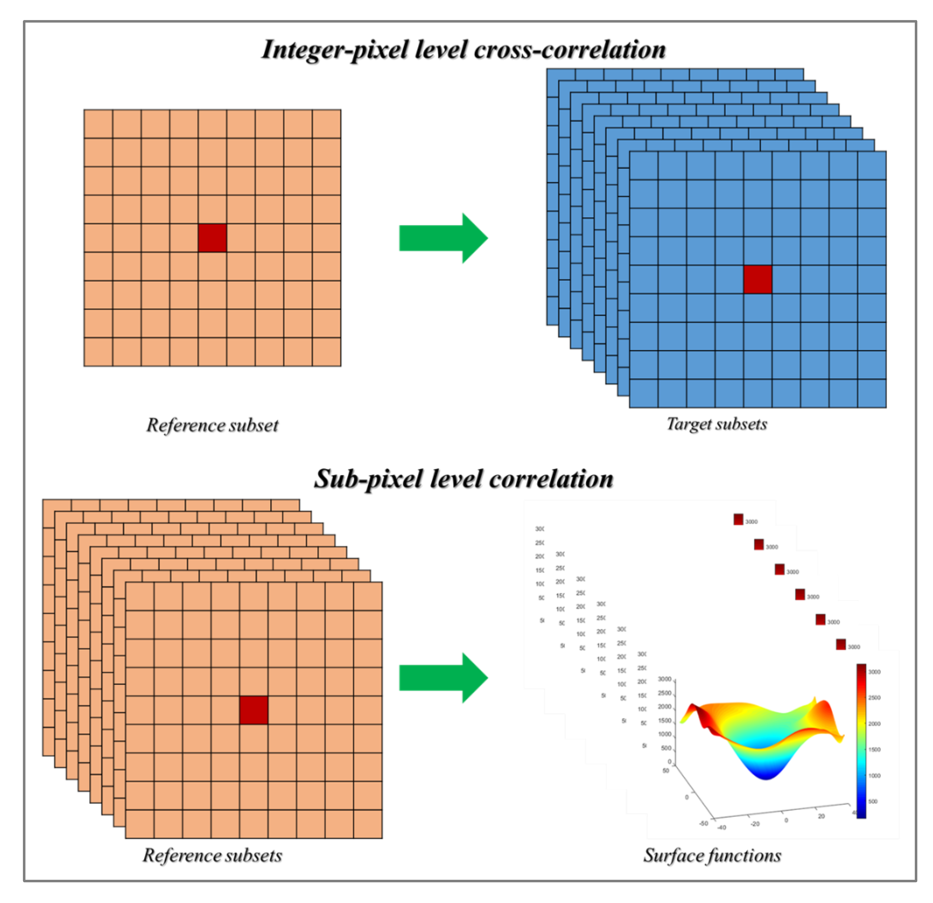
Resolution of the representation of discontinuous edges is improved by the use of high-density topography data, but this increases the solution time. For the purpose of dealing with this problem, GPU implementation of the hDIC technique was developed by defining subsets of reference and target conditions as pages of three-dimensional arrays as illustrated in Figure 1 for two stages of the hDIC technique.
Integer-pixel level cross-correlation stage aims to determine the best matching pixels between the topography data of reference and target conditions. Dimensions of subsets are formulated as where is an odd number in order to keep a single pixel in the centre of the subset. Cross-correlation is performed using the zero-mean normalised cross-correlation method which is formulated in Equation (1). In this equation, denotes the cross-correlation coefficient of subset, denotes the intensity of the pixel at coordinates in the reference subset, denotes the intensity of the pixel at coordinates in the target subset, denotes the mean intensity of the pixels in the reference subset and is the mean intensity of the pixels in the target subset. Three-dimensional array of target subsets is stored in the GPU memory to perform a parallel calculation of the zero-mean normalised cross-correlation coefficient of each reference subset with all target subsets.
Subsequent to the determination of the matching subsets, displacements are determined using the final coordinates of the matching pixels using Equation (2) where denotes the displacement in x-axis and denotes the displacement in y-axis.
After the integer-pixel level coarse-fine matching process, displacement noise for x- and y-components (in-plane) of displacements are removed by the bi-cubic B-form least-squares spline interpolation process. The interpolation scheme is employed using the spline function in terms of the weighed sum of B-splines as it is given in Equation (3) where is the and is the B-splines with a degree of in x- and y-axes, and are the number of control points in x- and y-axes and and are the coefficients in the dimensions of and . Smoothness of the spline function is determined by adjusting the number of control points. After the smoothing process, matching pixels in the target condition are updated with the coordinates calculated using the smoothed displacements.
In order to reduce the computation power demand, sub-pixel level correlation is accomplished around the matching pixels in the target condition. The search areas in the target condition are defined as separate cost functions using bi-cubic interpolation method which is given in Equation (4) where is the intensity at coordinates in the target and is the coefficient at the dimensions of and . The final equation, which has continuous derivatives [35], is distributed on a grid surface of unit squares.
Functions of the subsets of the target condition are reformulated as cost functions for sub-pixel level correlation process. The cost function of each target subset is determined using the interpolation function and the corresponding reference pixel, separately, using Equation (5) provided below.
The gradient descent minimisation process simultaneously updates the and coordinates in the surface, determined by the bi-cubic interpolation function, along the steepest descent direction using Equation (6) until the minimum is achieved. In this equation, represents the step size which is kept constant throughout the process. The GPU implementation of this process performs the creation of the cost functions and the gradient descent minimisation process for each reference subset, which are stored as a three-dimensional array in the GPU memory, in parallel.
3. Identification of Discontinuous Displacements
The hDIC technique was previously used to measure displacements on the aluminium tensile test specimen by the present authors [15]. The displacement measurements corresponding to the elastic region of the tensile test allowed calculation of Young’s modulus and Poisson’s ratio. Calculated elastic material properties and the linearity of the longitudinal component of the displacements validated the measurements of the hDIC technique. Smoothed displacement measurements in the plastic region were used to calculate strain distribution. However, that procedure of the hDIC did not provide any information about discontinuous displacements after the break. The GPU implementation of the hDIC technique with the new smoothing procedure was used for the identification of discontinuous displacements after the break of the same tensile test specimen. All calculations for the displacement calculations and benchmark tests were conducted with single precision.
3.1. Sample Preparation and Profilometry
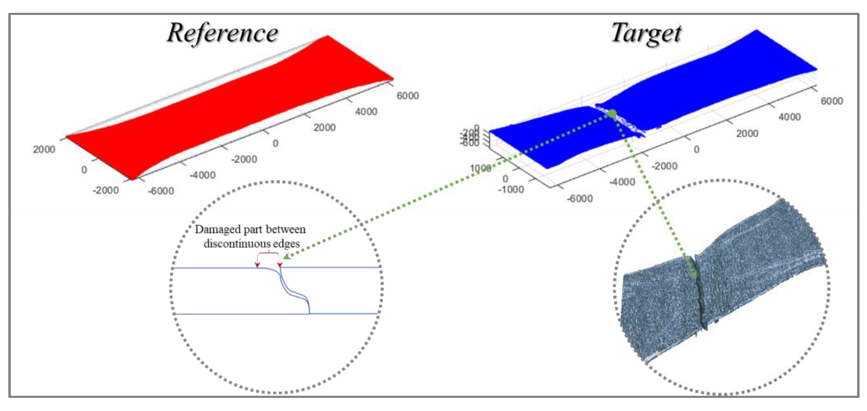
Tensile test specimen of aluminium alloy 6082/HE30 was prepared using the electric discharge machining technique which creates an electric arc that causes formation of pits with a depth of a few microns on the cut surface. Elastic modulus and Poisson’s ratio of HE 30 6082 aluminium are 70 GPa and 0.33, respectively. The tensile test specimen has a thickness of 2 mm and details of all dimensions can be found in the paper that presents the hDIC technique [15]. Tension load was applied using a 5kN tensile stage (Deben, Suffolk, UK) until the break and in situ surface profile scans were performed using an Infinite Focus 3D Profilometer instrument (Bruker Alicona, Graz, Austria). Vertical and lateral resolutions were kept as 200 nm and 8 µm, respectively, during the profilometry scans. Settings of the profilometer on the resolution was crucial, because it should be kept the same in order to satisfy repeatability. On the other hand, optical settings of the device were kept as default. Topography data corresponding to the reference and target conditions, as well as the information about the triaxial coordinates of the surface, are illustrated in Figure 2. The gap between the two sides after the break was minimised until the two edges got in touch, as illustrated in the circled images. The illustration in that figure shows that some parts of the broken edges are in touch. The top of the right side of the broken edge has a sharp jut along the top line while the symmetric line on the left side was buckled towards the centre of the material.
3.2. Determination of Optimum Subset Size and Smoothness
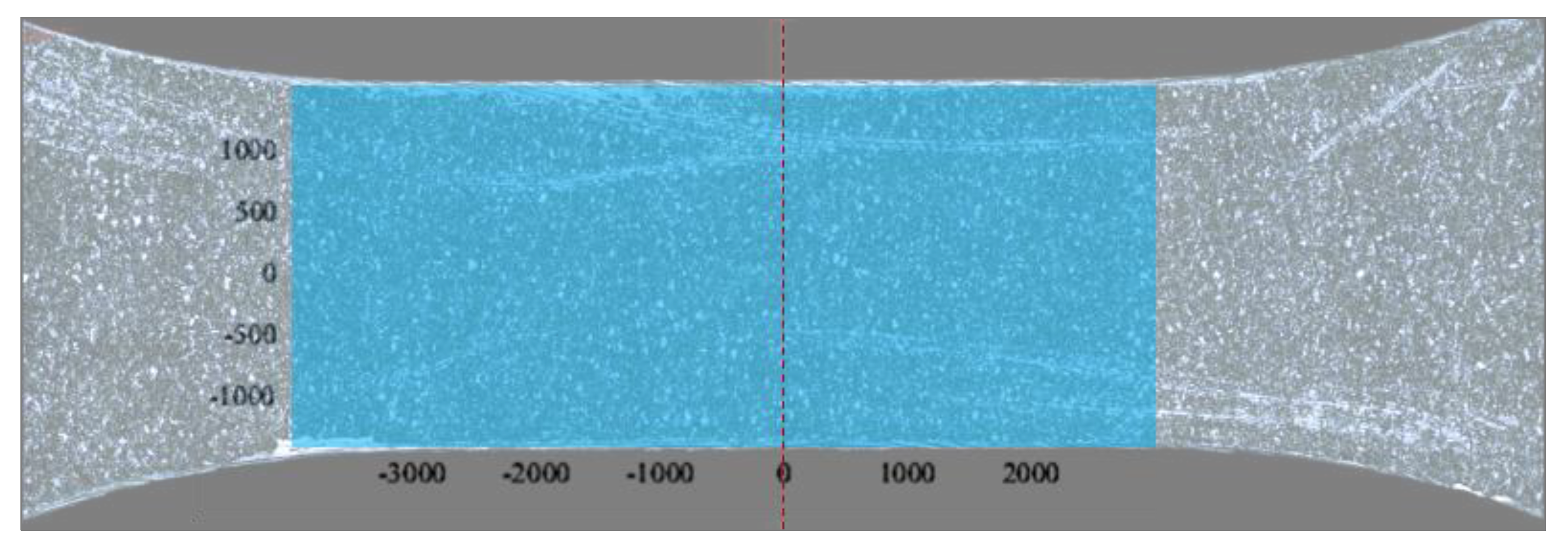
GPU implementation of the hDIC technique with the new smoothing procedure has two parameters that need to be determined carefully, which are smoothness and subset size. These parameters were investigated in terms of the coefficient of variation (CoV) of the error between the pixel intensities of the reference and the target condition. Optimum parameters are selected from the ones that provide the minimum CoV of the error. Tests were conducted by running both the integer-pixel and sub-pixel level correlation stages for each parameter using the same region of interest (ROI) which spreads from −4 mm to 3 mm along the longitudinal direction in the break zone with respect to the centre of the gauge, and covers the gauge width with a range of 3 mm, as illustrated in Figure 3.
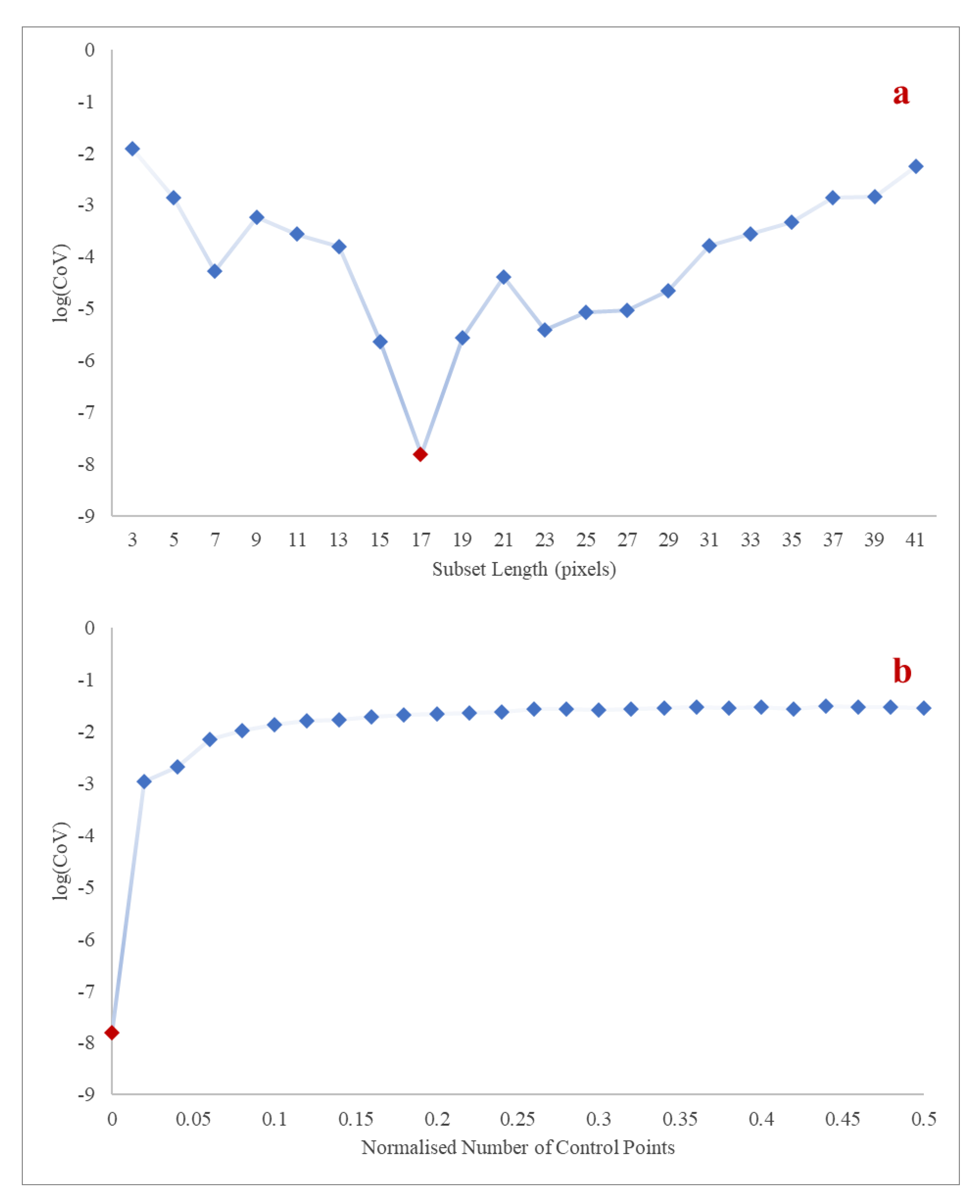
The first parameter is a subset size that should be determined carefully in order to calculate discontinuous displacements corresponding to the buckled and damaged sections of the break zone accurately, because the correlation on the damaged parts is expected to be accomplished by matching the pixels of the subset that belongs to the undamaged regions. The optimum subset size is determined by testing different subsets with a varying length of square, from 3 to 41 pixels, while keeping the smoothing parameter at maximum. Results of this analysis are given in Figure 4 in terms of the logarithm of the CoV. Minimum CoV is achieved when the subset length is 17 pixels, which corresponds to a subset of 289 pixels.
The second parameter is smoothness of the surface function that has crucial importance for cleaning the noisy displacement distribution and determination of the initial pixel for the iterations of sub-pixel level correlation stage. In this study, the purpose of the smoothing process is to create a function of smoothed results for the integer-pixel level correlation to predict coordinates of best matching pixels, but this smoothing process is not applied to the final results after the sub-pixel level correlation. The smoothness of the surface function created by the bi-cubic B-form least-squares spline interpolation [36] process is adjusted by the number of control points. Minimizing the number of control points increases the smoothness. In order to investigate the effect of smoothness on the CoV, smoothness is decreased to half, starting from the maximum smoothness while keeping the square subset length at 17 with 289 pixels. Results given in Figure 4 show that the minimum CoV is achieved when the smoothness is at maximum. However, this is achieved when the step size between subsets is one that means all pixels in the ROI were used in the correlation process.
3.3. Discontinuous Displacements after Break
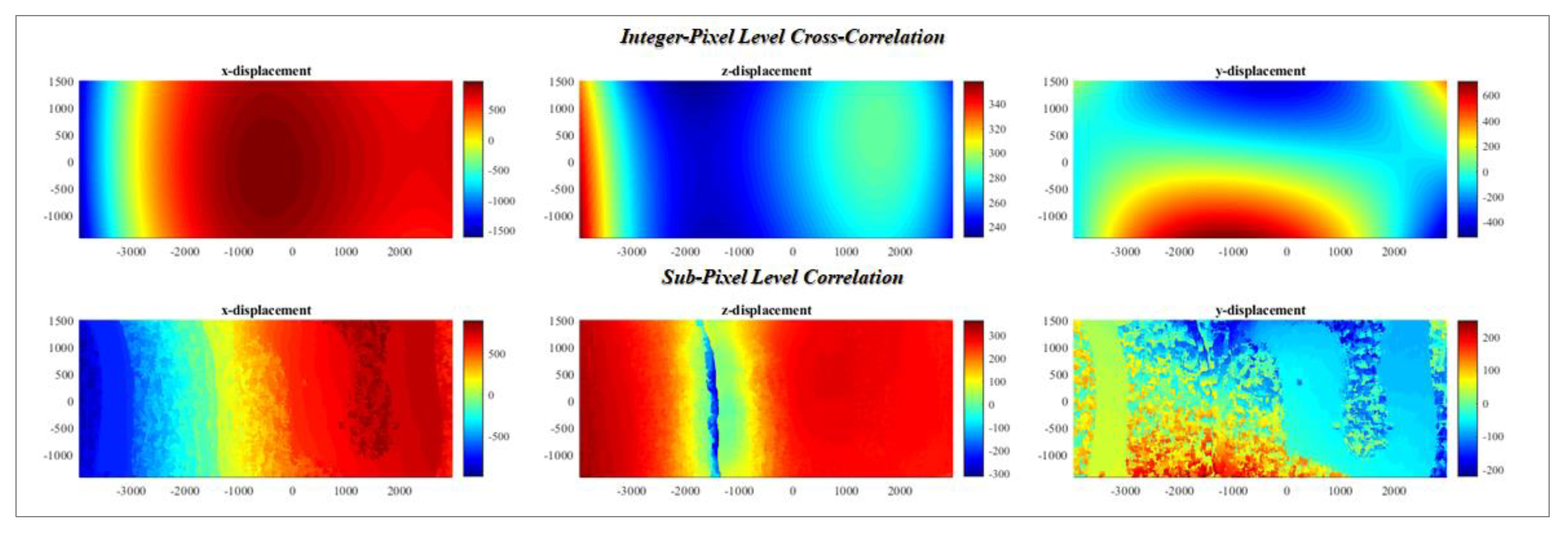
After the parameter analysis of GPU implementation of the hDIC technique with the new smoothing procedure, optimum subset length and smoothness were used to determine discontinuous displacements on the tensile test specimen after break. Figure 5 illustrates smoothed displacements determined after the integer-pixel level cross-correlation stage and the sub-pixel level correlation stage displacement calculations without smoothing on the undeformed shape of the ROI. Results show that the range between maximum and minimum values of displacement were changed, clusters of pixels that have similar displacements appeared and discontinuous edges were visible after the correlation. As expected, the path of the discontinuous edge on the right side of the break zone appeared in the illustrations of x- and z-displacements and the continuous increase in z-displacement, up to the path of the discontinuous edge, was observed on the left side of the break zone. The path of the discontinuous edge on the right side of the break zone is less visible in the illustration of y-displacement.
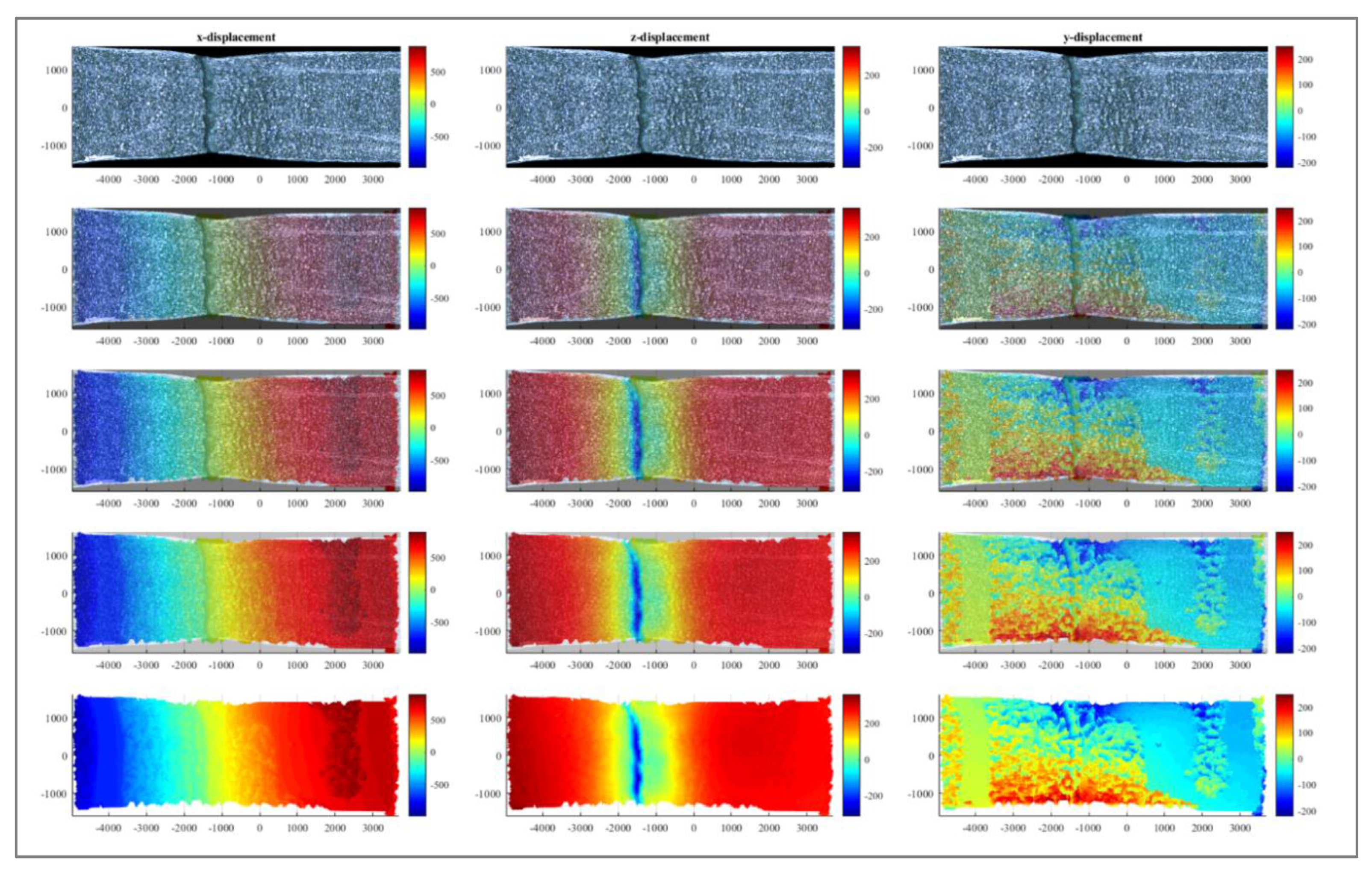
Displacements on the deformed shape of the ROI are illustrated as the transition from the microscopy image to the calculated displacements in Figure 6. This illustration shows the distribution of displacements on the deformed body calculated after the sub-pixel level correlation stage. Results of x- and z-displacements show a perfect match between the path of the discontinuous edge on the right side of the break zone in the microscopy image and the hDIC calculations. The discontinuous region becomes visible in the representation of all components of dispalcement but it becomes sharply visible in the z-displacement results seen in the middle column of Figure 6. This result shows the importance and benefits of using surface topography information for the purpose of the determination of discontinuous displacements.
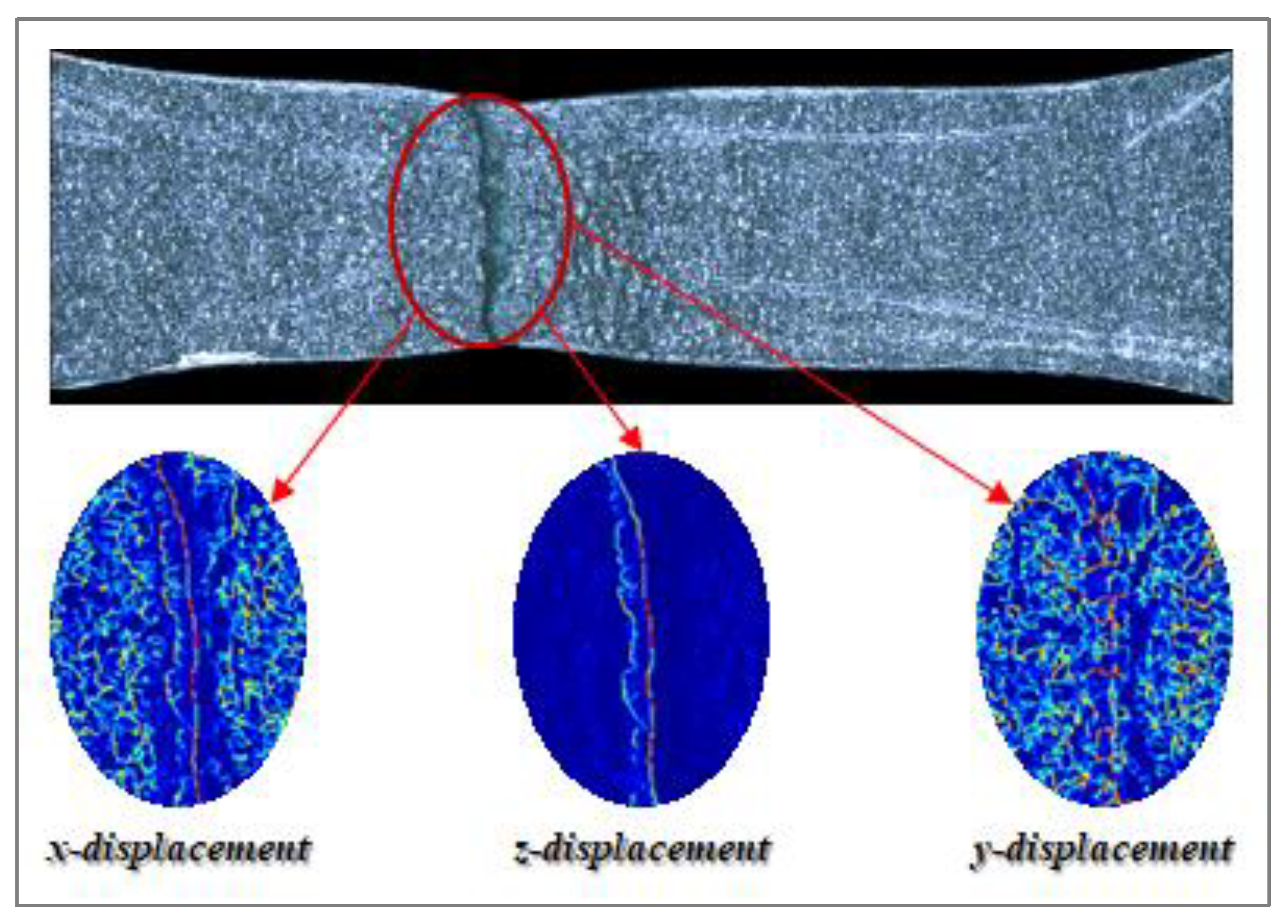
Local standard deviation around the break zone was calculated for better representation of discontinuous edges and illustrated in Figure 7. Coordinates on the microscopy image are the same with coordinates given in Figure 6 and in order to get a clear representation of the break zone, coordinates are not presented in this image. As expected, local standard deviations of x- and z-displacements provide a very clear view of the discontinuous edges on the right side of the break zone. The representation of local standard deviation of z-displacements also makes the beginning of the buckled field on the left side of the break zone visible, especially on the central parts of the gauge width, because in that region buckling is higher, but its distribution is not continuous.
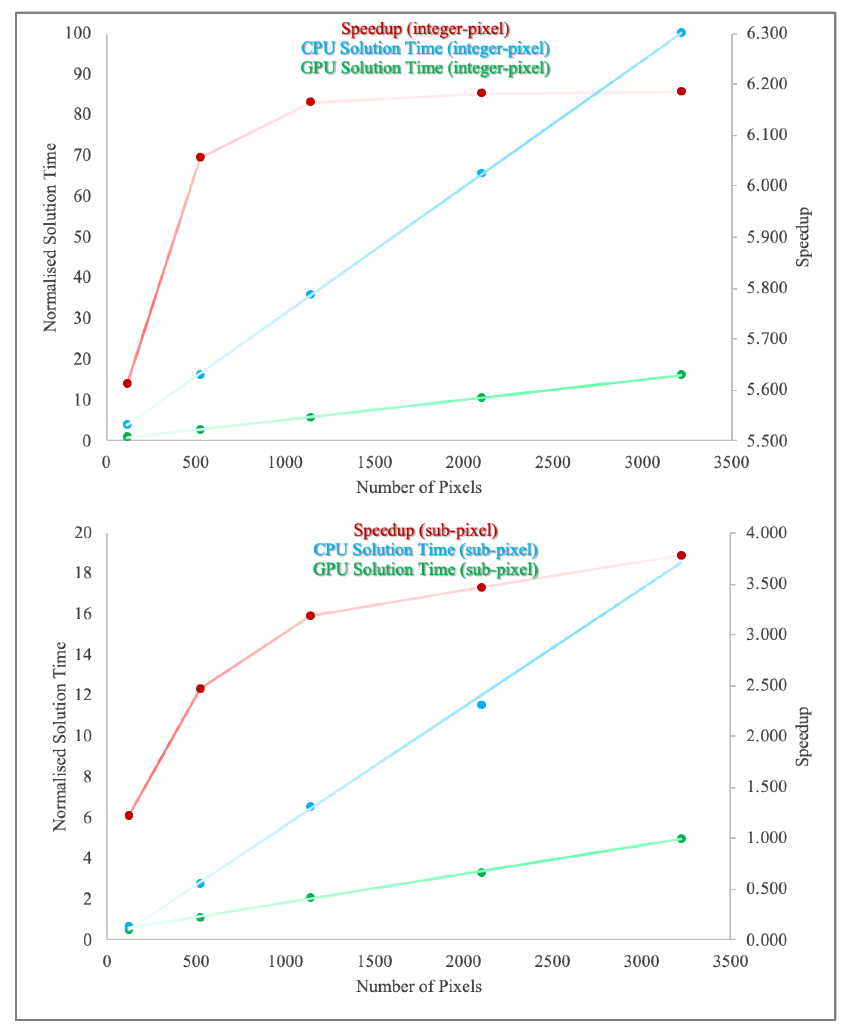
GPU parallel computing implementation of the hDIC technique was created based on Compute Unified Device Architecture (CUDA) parallel computing platform. In order to investigate the performance improvement gained by the GPU parallel computing, benchmark tests were conducted to compare serial calculations of Intel i7-8700 CPU (Intel, Santa Clara, CA, USA) and parallel calculations Nvidia Quadro P2000 GPU (Nvidia, Santa Clara, CA, USA). Tests were performed in ROIs with varying size and the results are illustrated in Figure 8. Normalised solution times show that the subpixel level correlation stage is completed five times faster in both CPU and GPU solutions which are linearly dependent on the number of pixels. The speedup gained by GPU parallel computing increases with the increasing number of pixels at each correlation stage. Maximum speedup is 6.2 times of the CPU calculations which was achieved when the ROI was created using the maximum number of pixels in the integer-pixel level cross-correlation stage.
Variation of the speedup in the sub-pixel level correlation stage shows that the increasing trend continues with increasing number of pixels, but the rate of the increase in the speedup decreases with increasing number of pixels. The speedup gained using this GPU has a potential to increase with increasing number of pixels in the sub-pixel level correlation stage, if the number of pixels is increased. The expectation for the maximum speed up in the sub-pixel level correlation stage is to reach a closer value obtained in the integer-pixel level correlation stage.
4. Conclusions
The hDIC technique was initially developed for the purpose of the determination of continuous displacement fields in three axes at the surface of a material using surface topography [15]. The proposed solution procedure of the hDIC technique and the use of the optimised subset size and smoothness allowed for the identification of discontinuous displacements involuntarily using surface topography information without any need for user interaction and guiding data. The new form of the hDIC technique correlates the surface topography information of reference and damaged states successfully in the regions where the material was buckled or broken. Boundaries of the discontinuous edges become sharply visible in the displacement results. The performance of the proposed method was improved by GPU implementation. The use of the paging method allowed us to speedup integer-pixel and sub-pixel level correlation stages. Visual representations of discontinuous edge on the right side of the break zone showed perfect agreement with the illustrations in microscopy image. Further improvements can be achieved by increasing the density of topography data.
Author Contributions
Conceptualization, F.U. and A.M.K; methodology, F.U. and A.M.K.; software, F.U.; validation, F.U. and A.M.K.; formal analysis, F.U.; writing-original draft preparation, F.U.; writing-review and editing, F.U. and A.M.K.; visualization, F.U.; supervision, A.M.K.; project administration, F.U.; funding acquisition, F.U. All authors have read and agreed to the published version of the manuscript.
Funding
This project has received funding from the European Union’s Horizon 2020 research and innovation programme under the Marie Skłodowska-Curie grant agreement No RESTREIG
Conflicts of Interest
The authors declare no conflict of interest.
Nomenclature
| coordinates in the target subset | |
| B-splines with a degree of | |
| B-splines with a degree of | |
| , | number of control points |
| denotes the mean intensity of the pixels in the reference subset | |
| mean intensity of the pixels in the target subset | |
| intensity of a pixel at coordinates | |
| coordinates in the reference subset | |
| , | coefficients of the spline function |
| coefficient at the dimensions of and | |
| , | dimensions of the spline function |
| an odd number to determine subset size | |
| intensity of a pixel at coordinates | |
| intensity of a pixel at coordinates | |
| displacement in x-axis | |
| displacement in y-axis | |
| step size of the gradient descent function |
References
- Parks, V.J. The range of speckle metrology. Exp. Mech. 1980, 20, 181–191. [Google Scholar] [CrossRef]
- Chu, T.C.; Ranson, W.F.; Sutton, M.A. Applications of digital-image-correlation techniques to experimental mechanics. Exp. Mech. 1985, 25, 232–244. [Google Scholar] [CrossRef]
- Hild, F.; Roux, S. Digital image correlation: From displacement measurement to identification of elastic properties—A review. Strain 2006, 42, 69–80. [Google Scholar] [CrossRef] [Green Version]
- Zhao, P.; Zsaki, A.M.; Nokken, M.R. Using digital image correlation to evaluate plastic shrinkage cracking in cement-based materials. Constr. Build. Mater. 2018, 182, 108–117. [Google Scholar] [CrossRef]
- Li, X.; Xu, W.; Sutton, M.A.; Mello, M. Nanoscale deformation and cracking studies of advanced metal evaporated magnetic tapes using atomic force microscopy and digital image correlation techniques. Mater. Sci. Technol. 2006, 22, 835–844. [Google Scholar] [CrossRef]
- Sun, Y.; Pang, J.H.L.; Fan, W. Nanoscale deformation measurement of microscale interconnection assemblies by a digital image correlation technique. Nanotechnology 2007, 18. [Google Scholar] [CrossRef]
- Xu, Z.H.; Sutton, M.A.; Li, X. Mapping nanoscale wear field by combined atomic force microscopy and digital image correlation techniques. Acta Mater. 2008, 56, 6304–6309. [Google Scholar] [CrossRef]
- Bruno, L. Full-field measurement with nanometric accuracy of 3D superficial displacements by digital profile correlation: A powerful tool for mechanics of materials. Mater. Des. 2018, 159, 170–185. [Google Scholar] [CrossRef]
- Vendroux, G.; Knauss, W.G. Submicron Deformation Field Measurements: Part 2. Improved Digital Image Correlation. Exp. Mech. 1998, 38, 86–92. [Google Scholar] [CrossRef]
- Bertin, M.; Du, C.; Hoefnagels, J.P.M.; Hild, F. Crystal plasticity parameter identification with 3D measurements and Integrated Digital Image Correlation. Acta Mater. 2016, 116, 321–331. [Google Scholar] [CrossRef] [Green Version]
- Wang, B.; Pan, B. Subset-based local vs. finite element-based global digital image correlation: A comparison study. Theor. Appl. Mech. Lett. 2016, 6, 200–208. [Google Scholar] [CrossRef] [Green Version]
- Hu, Z.; Xie, H.; Lu, J.; Hua, T.; Zhu, J. Study of the performance of different subpixel image correlation methods in 3D digital image correlation. Appl. Opt. 2010, 49, 4044–4051. [Google Scholar] [CrossRef] [PubMed]
- Pan, B.; Yu, L.P.; Zhang, Q.B. Review of single-camera stereo-digital image correlation techniques for full-field 3D shape and deformation measurement. Sci. China Technol. Sci. 2018, 61, 2–20. [Google Scholar] [CrossRef] [Green Version]
- Prakoonwit, S.; Benjamin, R. 3D surface reconstruction from multiview photographic images using 2D edge contours. 3D Res. 2012, 3, 1–12. [Google Scholar] [CrossRef]
- Uzun, F.; Korsunsky, A.M. The Height Digital Image Correlation (hDIC) Technique for the Identification of Triaxial Surface Deformations. Int. J. Mech. Sci. 2019, 159, 417–423. [Google Scholar] [CrossRef]
- van Beeck, J.; Neggers, J.; Schreurs, P.J.G.; Hoefnagels, J.P.M.; Geers, M.G.D. Quantification of Three-Dimensional Surface Deformation using Global Digital Image Correlation. Exp. Mech. 2014, 54, 557–570. [Google Scholar] [CrossRef] [Green Version]
- Sause, M.G.R. Digital image correlation. Springer Ser. Mater. Sci. 2016, 242, 57–129. [Google Scholar] [CrossRef]
- Abanto-Bueno, J.; Lambros, J. Investigation of crack growth in functionally graded materials using digital image correlation. Eng. Fract. Mech. 2002, 69, 1695–1711. [Google Scholar] [CrossRef]
- Mathieu, F.; Hild, F.; Roux, S. Identification of a crack propagation law by digital image correlation. Int. J. Fatigue 2012, 36, 146–154. [Google Scholar] [CrossRef] [Green Version]
- Mokhtarishirazabad, M.; Lopez-Crespo, P.; Moreno, B.; Lopez-Moreno, A.; Zanganeh, M. Evaluation of crack-tip fields from DIC data: A parametric study. Int. J. Fatigue 2015, 89, 11–19. [Google Scholar] [CrossRef]
- Hamam, R.; Hild, F.; Roux, S. Stress intensity factor gauging by digital image correlation: Application in cyclic fatigue. Strain 2007, 43, 181–192. [Google Scholar] [CrossRef]
- Mcneill, S.R.; Peters, W.H.; Sutton, M.A. Estimation of stress intensity factor by digital image coreelation. Eng. Fract. Mech. 1987, 28, 101–112. [Google Scholar] [CrossRef]
- Fayyad, T.M.; Lees, J.M. Application of Digital Image Correlation to Reinforced Concrete Fracture. Procedia Mater. Sci. 2014, 3, 1585–1590. [Google Scholar] [CrossRef] [Green Version]
- Chernyatin, A.S.; Matvienko, Y.G.; Lopez-Crespo, P. Mathematical and numerical correction of the DIC displacements for determination of stress field along crack front. Procedia Struct. Integr. 2016, 2, 2650–2658. [Google Scholar] [CrossRef] [Green Version]
- Jandejsek, I.; Gajdoš, L.; Šperl, M.; Vavřík, D. Analysis of standard fracture toughness test based on digital image correlation data. Eng. Fract. Mech. 2017, 182, 607–620. [Google Scholar] [CrossRef]
- Hosdez, J.; Witz, J.F.; Martel, C.; Limodin, N.; Najjar, D.; Charkaluk, E.; Osmond, P.; Szmytka, F. Fatigue crack growth law identification by Digital Image Correlation and electrical potential method for ductile cast iron. Eng. Fract. Mech. 2017, 182, 577–594. [Google Scholar] [CrossRef] [Green Version]
- Bourdin, F.; Stinville, J.C.; Echlin, M.P.; Callahan, P.G.; Lenthe, W.C.; Torbet, C.J.; Texier, D.; Bridier, F.; Cormier, J.; Villechaise, P.; et al. Measurements of plastic localization by heaviside-digital image correlation. Acta Mater. 2018, 157, 307–325. [Google Scholar] [CrossRef] [Green Version]
- Cinar, A.F.; Barhli, S.M.; Hollis, D.; Flansbjer, M.; Tomlinson, R.A.; Marrow, T.J.; Mostafavi, M. An autonomous surface discontinuity detection and quantification method by digital image correlation and phase congruency. Opt. Lasers Eng. 2017, 96, 94–106. [Google Scholar] [CrossRef]
- Uzun, F.; Salimon, A.I.; Statnik, E.S.; Besnard, C.; Chen, J.; Moxham, T.; Salvati, E.; Wang, Z.; Korsunsky, A.M. Polar transformation of 2D X-ray diffraction patterns and the experimental validation of the hDIC technique. Measurement 2019, 107193. [Google Scholar] [CrossRef]
- Craven, P.; Wahba, G. Smoothing noisy data with spline functions—Estimating the correct degree of smoothing by the method of generalized cross-validation. Numer. Math. 1978, 31, 377–403. [Google Scholar] [CrossRef]
- Woltring, H.J. On optimal smoothing and derivative estimation from noisy displacement data in biomechanics. Hum. Mov. Sci. 1985, 4, 229–245. [Google Scholar] [CrossRef]
- Palanca, M.; Tozzi, G.; Cristofolini, L. The use of digital image correlation in the biomechanical area: A review. Int. Biomech. 2016, 3, 1–21. [Google Scholar] [CrossRef]
- Li, X.; Zhao, J.; Shuai, J.; Zhang, Z.; Wu, X. Accurate Reconstruction of High-Gradient Strain Field in Digital Image Correlation: A Local Hermite Scheme. In Advancement of Optical Methods & Digital Image Correlation in Experimental Mechanics, Volume 3; Lamberti, L., Lin, M.-T., Furlong, C., Sciammarella, C., Reu, P.L., Sutton, M.A., Eds.; Springer International Publishing: Berlin/Heidelberg, Germany, 2019; pp. 173–175. [Google Scholar]
- Réthoré, J.; Gravouil, A.; Morestin, F.; Combescure, A. Estimation of mixed-mode stress intensity factors using digital image correlation and an interaction integral. Int. J. Fract. 2005, 132, 65–79. [Google Scholar] [CrossRef]
- Russell, W.S. Polynomial interpolation schemes for internal derivative distributions on structured grids. Appl. Numer. Math. 1995, 17, 129–171. [Google Scholar] [CrossRef]
- Amiri-Simkooei, A.R.; Hosseini-Asl, M.; Safari, A. Least squares 2D bi-cubic spline approximation: Theory and applications. Meas. J. Int. Meas. Confed. 2018, 127, 366–378. [Google Scholar] [CrossRef]
Figure 1.
GPU parallel computing implementation of two stages of the height digital image correlation (hDIC) technique.
Figure 1.
GPU parallel computing implementation of two stages of the height digital image correlation (hDIC) technique.

Figure 2.
Topography data of the reference and the target conditions with illustration of the buckled part on the left side of the break zone.
Figure 2.
Topography data of the reference and the target conditions with illustration of the buckled part on the left side of the break zone.

Figure 3.
Microscopy image of the reference condition of the tensile test specimen and illustration of position and dimensions of the region of interest (ROI) in units of micron, obtained using an Alicona Infinite Focus 3D Profilometer instrument.
Figure 3.
Microscopy image of the reference condition of the tensile test specimen and illustration of position and dimensions of the region of interest (ROI) in units of micron, obtained using an Alicona Infinite Focus 3D Profilometer instrument.

Figure 4.
Variation of logarithm of the coefficient of variation (CoV) with respect to subset length (a) and normalised number of control points (b). There is a connection between (a) and (b) parts of this figure. The analysis on normalised number of control points is performed using the best subset length obtained after the analysis on subset length.

Figure 5.
Results of the hDIC calculations after integer-pixel level cross-correlation and sub-pixel level correlation stages represented in the undeformed ROI in units of micron.
Figure 5.
Results of the hDIC calculations after integer-pixel level cross-correlation and sub-pixel level correlation stages represented in the undeformed ROI in units of micron.

Figure 6.
Illustration of the hDIC sub-pixel level displacement calculations in the deformed ROI and their transition from microscopy image of the deformed tensile test specimen in units of micron.
Figure 6.
Illustration of the hDIC sub-pixel level displacement calculations in the deformed ROI and their transition from microscopy image of the deformed tensile test specimen in units of micron.

Figure 7.
Illustration of local standard deviation of the hDIC displacement calculations around the break zone.
Figure 7.
Illustration of local standard deviation of the hDIC displacement calculations around the break zone.

Figure 8.
Results of the benchmark tests in terms of normalised solution times of serial CPU and parallel GPU computing.
Figure 8.
Results of the benchmark tests in terms of normalised solution times of serial CPU and parallel GPU computing.

© 2020 by the authors. Licensee MDPI, Basel, Switzerland. This article is an open access article distributed under the terms and conditions of the Creative Commons Attribution (CC BY) license (http://creativecommons.org/licenses/by/4.0/).
Share and Cite
MDPI and ACS Style
Uzun, F.; Korsunsky, A.M. The Use of Surface Topography for the Identification of Discontinuous Displacements Due to Cracks. Metals 2020, 10, 1037. https://doi.org/10.3390/met10081037
AMA Style
Uzun F, Korsunsky AM. The Use of Surface Topography for the Identification of Discontinuous Displacements Due to Cracks. Metals. 2020; 10(8):1037. https://doi.org/10.3390/met10081037
Chicago/Turabian StyleUzun, Fatih, and Alexander M. Korsunsky. 2020. "The Use of Surface Topography for the Identification of Discontinuous Displacements Due to Cracks" Metals 10, no. 8: 1037. https://doi.org/10.3390/met10081037
Note that from the first issue of 2016, this journal uses article numbers instead of page numbers. See further details here.