The Strong Resolving Graph and the Strong Metric Dimension of Cactus Graphs


Departamento de Estadística e Investigación Operativa, Universidad de Cádiz, 11003 Cádiz, Spain
Mathematics 2020, 8(8), 1266; https://doi.org/10.3390/math8081266
Submission received: 29 April 2020
/
Revised: 12 July 2020
/
Accepted: 21 July 2020
/
Published: 2 August 2020
(This article belongs to the Special Issue Distances and Domination in Graphs)
Abstract
:A vertex w of a connected graph G strongly resolves two distinct vertices , if there is a shortest path containing v, or a shortest path containing u. A set S of vertices of G is a strong resolving set for G if every two distinct vertices of G are strongly resolved by a vertex of S. The smallest cardinality of a strong resolving set for G is called the strong metric dimension of G. To study the strong metric dimension of graphs, a very important role is played by a structure of graphs called the strong resolving graph In this work, we obtain the strong metric dimension of some families of cactus graphs, and along the way, we give several structural properties of the strong resolving graphs of the studied families of cactus graphs.
Keywords:
strong resolving graph; strong metric dimension; strong resolving set; cactus graphs; unicyclic graphsMSC:
05C121. Introduction
Topics concerning metric dimension and related parameters in graphs are nowadays very common in the research community, probably based on its applicability to diverse practical problems of identification of nodes in networks. One can find in the literature a large number of works dealing with this topic, both from the applied and theoretical points of views. A popular research line in this subject concerns studying different variants of metric dimension in graphs, which have had their beginnings in the seminal standard metric dimension concept. Some of the most recent ones are probably the edge metric dimension [1], the mixed metric dimension [2], the k-metric antidimension [3], the strong partition dimension [4], and the multiset dimension [5,6], just to cite a few recent and remarkable cases. One other interesting version is the strong metric dimension [7], which is now relatively well studied, although a few open questions on this are still open. A fairly complete study on results and open questions concerning the strong metric dimension of graphs can be found in [8].
One significant reason for the interest of several researchers in the strong metric dimension of graphs concerns the closed relationship that exists between such parameter and the very well known vertex cover number of graphs (and thus with the independence number, based on the Gallai’s Theorem). To see this relationship, for a given graph G, the construction of a new related graph, called strong resolving graph, was required. This graph transformation clearly raised some other related questions on the transformation itself. That is for instance, given a graph G: can some properties of the strong resolving graph of G be deduced? or; can we realize every graph H as the strong resolving graph of another graph ? These ones and several other questions were dealt with in [9], which was the first work paying specific attention to the strong resolving graphs of graphs as a special graph transformation. See also [10], where an open problem from [9] was settled.
Clearly, and as we will further notice, a good knowledge of the strong resolving graph of a graph brings important contributions to studying the strong metric dimension of graphs. In this sense, this work is precisely aimed to study the strong resolving graphs and the strong metric dimension of cactus graphs, with some emphasis on different special structures of such cactus graphs. As one will also note through our exposition, strong resolving graphs are very challenging for those graphs having a large number of induced cycles. Thus, cactus graphs represent a significant example of such a situation. With this work, we also contribute to some open problems presented in [9].
The study of the strong metric dimension of some classes of cactus graphs was started in [11,12] where the authors presented some general results for the strong metric dimension of corona product graph and rooted product graphs, respectively. Clear definitions of these two graph products can be found in [8]. A corona product graph or a rooted product graph can have the structure of a cactus graph, depending on which are the graphs used as factors in the product. For instance, if G is a cycle and H is a graph whose components are only singleton vertices or complete graphs , then it happens that the corona product graph is a cactus graphs. To generate a rooted product graph that is a cactus graph, we may consider for example two graphs G and H which are paths or cycles.
On the other hand, we must mention that the strong metric dimension of unicyclic graphs (which is a cactus graph too) was studied in [13]. There, among other results, several relationships between the strong metric dimension of a unicyclic graph and that of its complement were given. A few other sporadic results can be found in some other articles dealing with related topics that could include examples of cactus graphs. However, we prefer to not include more references that are not essentially connected with this article.
We hence now begin to formalize all the required notations and terminologies that shall be used throughout the document. To this end, for the whole exposition, let G be a connected simple graph with vertex set . For two adjacent vertices , we use the notation . For a vertex x of G, denotes the set of neighbors that x has in G, i.e., . The set is called the open neighborhood of a vertex x in G and is called the closed neighborhood of a vertex x in G. The degree of the vertex x is . The diameter of G is defined as , where is the length of a shortest path between x and y (a shortest path). Two vertices are called diametral if . For a set , by we represent the subgraph induced by S in G.
1.1. Strong Metric Dimension of Graphs
For two distinct vertices , a vertex strongly resolves if there is a shortest path containing v, or a shortest path containing u. Note that it could happen . A set S of vertices of G is a strong resolving set for G, if every two vertices of G are strongly resolved by some vertex of S. The smallest cardinality among all strong resolving sets for G is called the strong metric dimension of G, and is denoted by . We say that a strong resolving set for G of cardinality is a strong metric basis of G. It next appears the value of the strong metric dimension of some basic graphs.
Observation 1.
Let G be a connected graph G of order .
- (a)
- if and only if .
- (b)
- If , then .
- (c)
- if and only if .
- (d)
- If , then .
- (e)
- If G is a tree with l leaves, .
It is said that a vertex u of G is maximally distant from v if for every , it happens . If u is maximally distant from v and v is maximally distant from u, then u and v are mutually maximally distant, and we write that are MMD in G. The set of MMD vertices of G is denoted by . Note that the set of MMD vertices of a graph G is also known as the boundary of G, as defined in [14,15]. An explanation on the equivalence of these two objects can be readily observed, but also found in [16]. From these definitions, the following remarks are straightforward to observe.
Remark 1.
Let G be a connected graph. Then every two vertices with degree 1 are MMD in G.
For any two mutually maximally distant vertices in G, there is no vertex of G that strongly resolves them, except themselves. This allows to claim the following.
Remark 2.
For every pair of mutually maximally distant vertices of a connected graph G, and for every strong metric basis S of G, it follows that or .
1.2. Strong Resolving Graph of a Graph
Given a connected graph G, the strong resolving graph of G, denoted by , has vertex set and two vertices are adjacent if and only if u and v are MMD in G. We must remark that the strong resolving graph of a graph G was defined in [7] as the graph with vertex set and two vertices are adjacent if and only if u and v are MMD in G. Observe that the difference between these two definitions is the existence of isolated vertices in the strong resolving graph from [7]. The main reason of using in this work the slightly different version is to have a simpler notation and more clarity while proving the results. Moreover, this fact does not influence on the computations we made.
For several basic families of graphs, describing their strong resolving graphs is a straightforward problem. We next recall some examples, which will maybe further useful, and to this end, we recall that a vertex v of a graph G is simplicial, if its closed neighborhood induces a complete graph, and also that a graph G is 2-antipodal if every vertex of G is diametral with exactly one other vertex of G.
Observation 2.
- (a)
- If equals the set of simplicial vertices of G, then . In particular, and for any tree T, .
- (b)
- For any 2-antipodal graph G of order n, . In particular, .
- (c)
- For odd cycles .
- (d)
- For any complete k-partite graph such that , , .
In [9], realization and characterization problems of the strong resolving graph of a graph as a graph transformation were firstly dealt with. That is, the following problems were studied.
- Realization Problem. Determine which graphs have a given graph as their strong resolving graphs.
- Characterization Problem. Characterize those graphs that are strong resolving graphs of some graphs.
For instance, in [9] was proved that complete graphs, paths and cycles of order larger than four are realizable as the strong resolving graph of other graphs. On the other hand, it was also proved in [9] that stars and cycles of order four are not realizable as strong resolving graphs. Based on these two facts, a conjecture concerning the not realization of complete bipartite graphs in general was pointed out. Such conjecture was recently shown in [10].
In connection with these comments, it would be desirable to continue obtaining some realization (and also characterization - although much more complicated) results for the strong resolving graphs of graphs. We are then aimed in this work to present some realization results which are involving cactus graphs.
1.3. Strong Metric Dimension of G versus Vertex Cover Number of
Oellermann and Peters-Fransen [7] showed that the problem of finding the strong metric dimension of graphs can be transformed into the well-known problem regarding the vertex cover of graphs. A set S of vertices of G is a vertex cover of G if every edge of G is incident with at least one vertex of S. The vertex cover number of G, denoted by , is the smallest cardinality of a vertex cover of G. We refer to a -set in a graph G as a vertex cover set of cardinality .
Theorem 1
Recall that the largest cardinality of a set of vertices of G, no two of which are adjacent, is called the independence number of G and is denoted by . We refer to an -set in a graph G as an independent set of cardinality . The following well-known and useful result, due to Gallai, states the relationship between the independence number and the vertex cover number of a graph.
Theorem 2
(Gallai’s theorem). For any graph G of order n,
Thus, by using Theorems 1 and 2 we immediately obtain the next result.
Corollary 1.
For any graph G,
2. Cactus Graphs: General Issues
A cactus graph (also called a cactus tree) is a connected graph in which any two simple cycles have at most one vertex in common. Equivalently, every edge of the graph belongs to at most one simple cycle. Next we study the strong metric dimension of cactus graphs, and we first give some necessary terminology. Note that a cycle of two vertices is precisely a path on two vertices. A vertex belonging to at least two simple cycles is a cut vertex. A cycle having only one cut vertex is called a terminal cycle. In a terminal cycle A, every vertex being diametral, in the subgraph induced by A, with respect to the cut vertex of A is a terminal vertex. From now on, denotes the set of terminal vertices of G. Also, denotes the set of vertices v, of degree two, belonging to a cycle of order larger than two, being MMD only with vertices of the same cycle which v belongs. Moreover, denotes the set of vertices u, of degree two, belonging to a cycle of order larger than two being MMD with at least one vertex of a different cycle which u belongs. The following remark can be easily observed.
Remark 3.
Let G be a cactus graph. Then, two vertices are MMD in G if and only if .
Corollary 2.
For any cactus graph G, .
Theorem 3.
Let G be a cactus graph. Then
Proof.
The lower bound follows from the following facts. Any two terminal vertices of G are MMD on G, and thus, they induce a complete graph of order . Also, vertices of induce at least a graph with independent edges that need to be covered in . Thus, one needs at least to strongly resolve all the vertices of G.
To see the upper bound, it is only necessary to observe that the set together with half of vertices of the set form a strong resolving set of G, and so, we are done. □
Despite the fact that the bounds above are easily proved, we might notice that the problem of describing the strong resolving graph, and similarly, of computing the strong metric dimension of cactus graphs seems to be very challenging based on the situation that we can not control things like the orders of the involved cycles, the number of terminal vertices and cut vertices, their adjacencies, etc. In this sense, it is desirable to introduce extra conditions on the cactus graphs to have more possibilities to give some practical results.
3. Strong Resolving Graphs
In this section we aim to describe the structure of the strong resolving graphs of several different families of cactus graphs. We specifically center our attention into unicyclic graphs, bouquet of cycles and chains of even cycles. With some of these results we contribute to the problem of realization of some graphs as strong resolving graphs, that is, to the problems previously presented.
3.1. Unicyclic Graphs
Given a unicyclic graph G different from a cycle, from now on we will denote by the subgraph induced by the unique cycle of G. A vertex of degree one is a terminal vertex of G, and is the set of terminal vertices of G. Note that the terminal vertices defined here represent a particular case of the terminal vertices defined for cactus graphs in general. If the vertex of has degree greater than two, then we say that is a terminal vertex of , if . The set of terminal vertices of a vertex is denoted by . We will denote by the set of vertices of the cycle having degree two. If , then we will say that .
Notice that if the unicyclic graph G is isomorphic to the cycle , then for n even and for n odd as already presented in Observation 2. Thus, we will study the cases that .
We begin with the following straightforward observations that are useful to describe the strong resolving graph of any unicyclic graph.
Remark 4.
Let G be a unicyclic graph. For every vertex there exists at least one vertex such that are MMD in G.
Remark 5.
Let G be a unicyclic graph. Then two vertices are MMD in G if and only if .
Corollary 3.
For any unicyclic graph G, .
Notice that every two vertices are MMD. Also, every vertex is MMD with every vertex w satisfying one of the following conditions.
- w is a terminal vertex of a vertex u of such that are diametral vertices in .
- w is a diametral vertex with v in and .
As a consequence of the above comments, we can deduce the structure of the strong resolving graph of any unicyclic graph G in the following way. First notice that, according to Corollary 3, has vertex set equal to , and to describe the adjacency of vertices in we consider two cases.
for r even.
- The set forms a clique in and each vertex of has at most one neighbor in .
- If are diametral vertices in , then is a connected component of isomorphic to .
- If are diametral vertices in , and , then forms a subgraph of isomorphic to and .
As a consequence of the description above, we can observe that .
for r odd.
- The set forms a clique in and each vertex of has at most two neighbors in .
- Let and let being diametral vertices with u in .
- –
- If , then is a subgraph of isomorphic to , and for every , .
- –
- If , then is a subgraph of isomorphic to , and for every , for (notice that if , then ).
- –
- If and , then the set form a subgraph (not induced) (Notice that the vertices are adjacent between them in .) of isomorphic to a star graph with central vertex u, , and for every , .
Similarly to the case when r is even, we can observe here that .
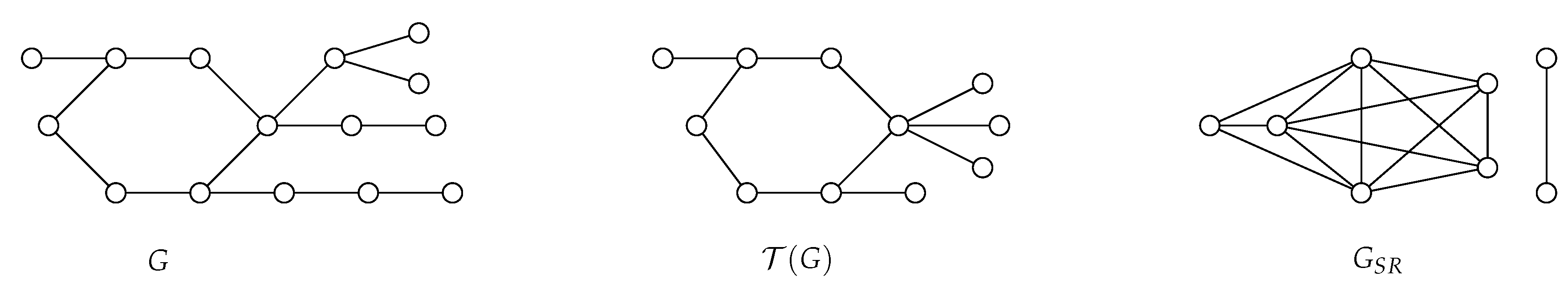
We define the branch restricted unicyclic graph associated to a unicyclic graph G in the following way. We begin with taking the cycle in G and removing the remaining vertices of G. Then we add pendant edges to every vertex in . Figure 1 shows an example of a unicyclic graph, its branch restricted unicyclic graph and its strong resolving graph.
Lemma 1.
Let G be a unicyclic graph and be its branch restricted unicyclic graph. Then is isomorphic to
Proof.
From Remarks 4 and 5, and by the definition of the branch restricted unicyclic graph, we deduce that is isomorphic to . □
Our next step is dedicated to present a realization result for some corona product graphs, where the solution precisely involves the use of unicyclic graphs. We first recall that the corona product graph is defined as the graph obtained from a graph G of order n and a graph H, by taking one copy of G and n copies of H, and then joining by an edge each vertex from the -copy of H with the -vertex of G.
Proposition 1.
For any integer , there exists a graph G such that .
Proof.
We consider the unicyclic graph G with a cycle such that the vertices , , …, form the set and the remaining ones from the cycle have exactly one terminal vertex. Since is an even number according to the Description of it clearly follows that is isomorphic to where each vertex of has exactly one neighbor in . □
3.2. Bouquet of Cycles
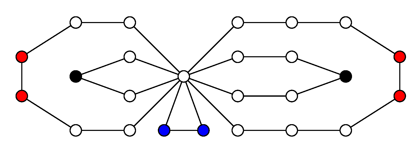
Let be a family of graphs obtained in the following way. Each graph is a bouquet of cycles where a of them are even cycles (of order at least four), b are odd cycles of order larger than three, c are cycles of order three, , and . All cycles of have the common vertex w. One example of a bouquet of cycles is given in Figure 2. Let be the even cycles of order at least four in and be the odd cycles of order larger than three in .
In [17], the authors have described the structure of the strong resolving graph of the graph as follows. By completeness of our exposition, we copy exactly the description presented there, since it makes no sense to do some changes on it, as it is fairly well written.
- The set of vertices of each odd cycle , , which are different from w induces a path of order , in , whose leaves are the two vertices that are diametral with w.
- The set of vertices of each cycle , , which are not diametral with w induces a graph isomorphic to the disjoint union of complete graphs in .
- Every three vertices such that , and are pairwise adjacent.
If we study the bouquet of cycles with (or equivalently, B has not odd cycles of order larger than three), and are the cycles of even order, then the strong resolving graph is composed by the complete graph and components isomorphic to .
Now, we again give some realization results for strong resolving graphs. To this end, we need to define a graph structure which we call a partial multisubdivided complete graph . That is, a complete graph where each edge of a perfect matching of this graph is subdivided times for (the case when some means that the edge corresponding to is not subdivided). Moreover, recall that the cocktail party graph , also called the hyperoctahedral graph, is a regular graph on n vertices.
Proposition 2.
For any integer , there exists a graph G such that is isomorphic to .
Proof.
We consider the bouquet of cycles with , and are the cycles of odd order larger than three. According to the construction of the strong resolving graph , the subgraph is isomorphic to and the set of vertices of each odd cycle , , which are different from w induces a path of order , in , whose leaves are the two vertices of this cycle that are not adjacent in . □
Corollary 4.
For any integer , there exists a graph G such that contains the cocktail party graph as an induced subgraph.
3.3. Chains of Even Cycles
A chain of cycles is a cactus graph in which, every cycle has order at least three and there are only two terminal cycles. Notice that in such case every non-terminal cycle has exactly two cut vertices, such that each cut vertex belongs to exactly two cycles. We next center our attention into the case of chains of even cycles. To this end, we need some terminology and notation. A chain of even cycles is a straight chain, if the cut vertices of every cycle in the chain are diametral in the cycle. Note that each straight chain contains two diametral vertices, which are the unique terminal vertices of this chain.
For the purposes of simplifying, given an integer , we shall define the next family of graphs. Each graph is a chain of even cycles constructed as follows.
- We begin with straight chains of even cycles, say , satisfying that the last cycle of the straight chain is isomorphic to the first cycle of the straight chain for every .
- Assume that the last cycle of each straight chain is , for every . By the item above, this (in ) is isomorphic to the first cycle of the straight chain with .
- Assume also that the terminal vertices of each straight chain are , for every .
- To construct our chain of even cycles , for every , we identify the last cycle of with the first cycle of (that are isomorphic) as follows. Every vertex of is identified with the vertex for some and every (operations with the subindex of v are done modulo r).
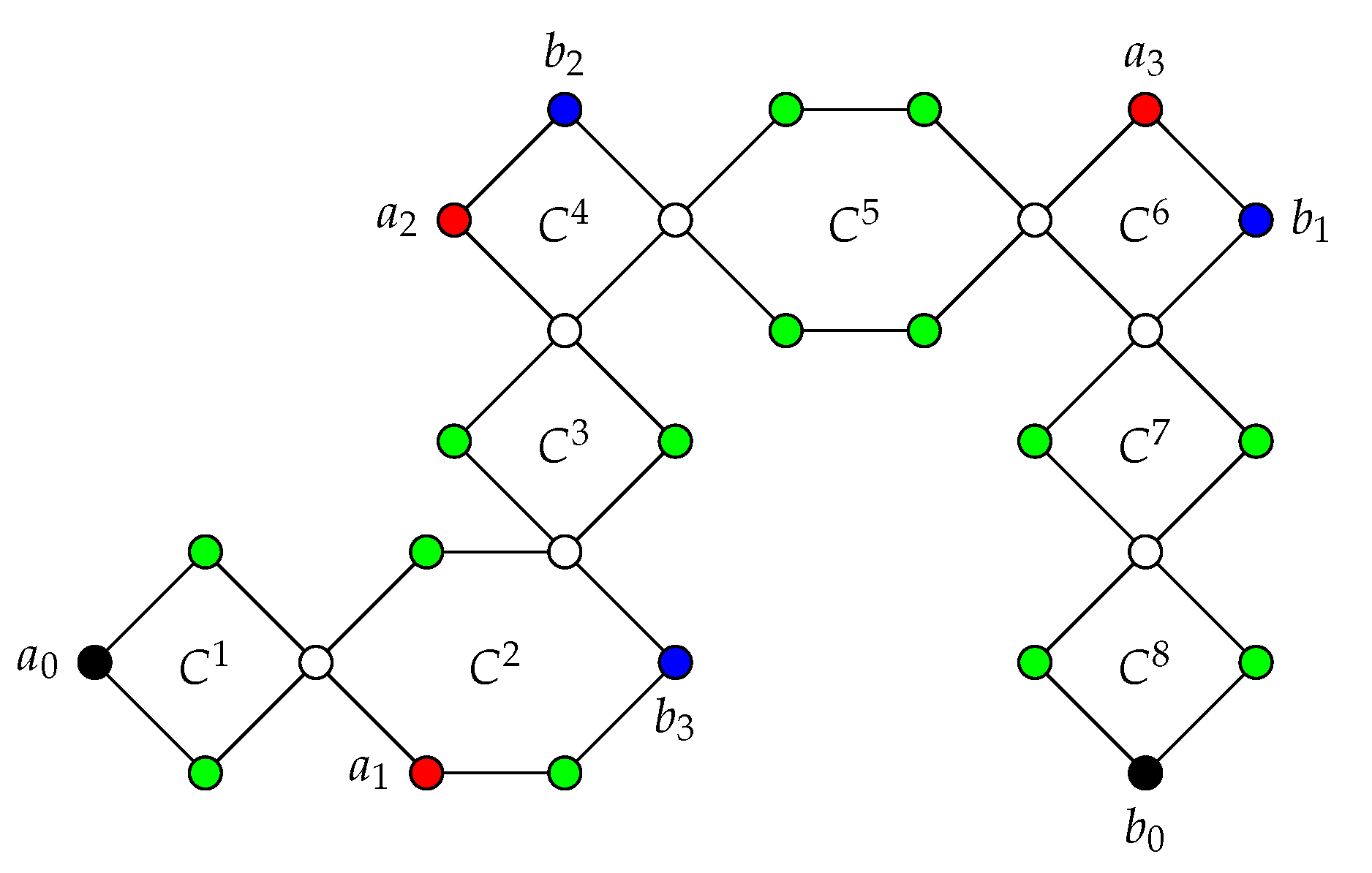
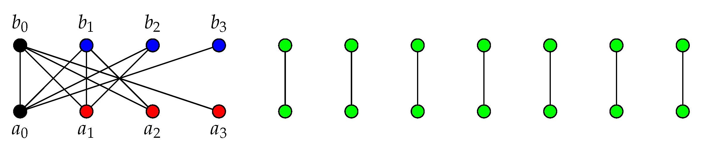
Notice that for instance, for the chain of even cycles described above, the two terminal vertices of it are and . Figure 4 shows a fairly representative example of a chain of even cycles. Recall that the way of drawing such graph (with respect to directions of the “turns” in the chain) does not influence in our purposes. The chain of even cycles presented in the Figure 4 has four straight chains of even cycles: contains and , contains , and , contains , and , and contains , and .
We next describe the strong resolving graph of a chain of even cycles . We need first the following observations.
Remark 6.
For any chain of even cycles , a vertex x belongs to if and only if x has degree two.
Remark 7.
In a straight chain of cycles, the two terminal vertices form a pair of MMD vertices, as well as each pair of diametral vertices in each cycle.
Observation 3.
For a chain of even cycles , and for every and it follows.
- The terminal vertex of the straight chain is MMD with every vertex of the straight chain .
- The terminal vertex of the straight chain is MMD with every vertex of the straight chain .
- In any cycle of F, any pair of diametral (in the cycle) vertices being not cut nor terminal vertices of F are MMD.
For instance, in Figure 4, the red vertex is MMD with the blue vertices , while the blue vertex is MMD with the red vertices . Moreover, again in Figure 4, any pair of green diametral vertices belonging to the same cycle are MMD in F.
With these observations above, we are able to describe the structure of for every chain of even cycles . To do so, we shall need the following construction, which represents a bipartite graph of order for some . The two bipartition sets of the bipartite graph are the sets and . The edges of are as follows. For every and every , there exist the edges and .
- The set of vertices and , with , forms a component of the graph isomorphic to a bipartite graph .
- In each cycle of F, each pair of diametral vertices in the cycle, not including terminal nor cut vertices, induces a graph isomorphic to in .
We may remark that, the strong resolving graph of a straight chain of cycles is simply a union of several complete graphs . The strong resolving graph of the chain of even cycles shown in Figure 4 is drawn in Figure 5.
We end this subsection by giving a realization result for strong resolving graphs involving chains of even cycles.
Corollary 5.
For any integer , there exists a chain of even cycles such that contains the bipartite graph as a component.
4. The Strong Metric Dimension
We are next centered into computing or bounding the strong metric dimension of the cactus graphs which we have studied in the previous section.
4.1. Unicyclic Graphs
Our first results shows the relationship between the strong metric dimension of a unicyclic graph and that of its branch restricted unicyclic graph.
Lemma 2.
Let G be a unicyclic graph and be its branch restricted unicyclic graph. Then
Proof.
By Lemma 1 and Theorem 1, we derive that and the proof is complete. □
Theorem 4.
Let G be a unicyclic graph with unique cycle . Then
Proof.
From Remark 1 we have that every strong resolving basis must contain at least vertices of degree one. So, . On the other hand, for every vertex there exists at least a vertex such that (notice that it could happen ). Thus we have that .
On the other side, since forms a clique in and for every there exists at least one vertex such that they are MMD, according to the description of presented in the previous section, we have . Therefore the proof is complete. □
As we can see in the following, the bounds above are tight. In particular, we characterize all the unicyclic graphs having a unique cycle of even order that are attaining the upper bound.
Theorem 5.
Let G be a unicyclic graph with a unique cycle of even order. Then if and only if .
Proof.
We assume . Let v be the only vertex of with degree greater than two, and let u be the diametral vertex with v in . So, every two vertices in are MMD. Also, every two diametral vertices in are MMD. Thus, is formed by connected components isomorphic to and one component isomorphic to . Since , we have that
We assume now that is satisfied. If , then there are at least two vertices such that and . We consider two cases.
Case 1: are diametral in . Hence, forms a clique in of cardinality . Also, the vertices in have no neighbor from in . Note that, there could be some other vertices in having neighbors from in , and if there is one of such vertices, say z, then and is also a clique in . However, this will not influence on the fact that, in order to cover the edges of , one can leave one vertex w of outside of the vertex cover set, by simply taking as a part of such vertex cover set. Thus, we have that , a contradiction.
Case 2: are not diametral in . Let being diametral vertices with , respectively. Hence, , and form cliques in . Also, have no neighbor in other than that ones in , respectively. Thus, in order to cover the edges of , we can leave outside of the vertex cover set both vertices , by simply taking in such vertex cover set. On the other hand, to cover the remaining vertices in we will need at most . We then deduce that , a contradiction again.
Since we have contradiction on both cases above, it must happen that , and the proof is completed. □
Note that the upper bound of Theorem 4 is also tight when the unique cycle of G is odd, but the characterization of the limit case seems to be a hard working task. For instance, if G has a unique cycle of odd order and , then a “relatively” similar argument to the first part of the proof of Theorem 5 leads to conclude that . Other cases, when can be hand computed, and we leave this to the reader.
Proposition 3.
Let G be a unicyclic graph with a unique cycle of even order. Then if and only if the following items hold.
- (i)
- for every x of .
- (ii)
- There is at most one pair of diametral vertices in each one having one terminal vertex.
Proof.
Assume . If for some x of , then let be the vertex of being diametral with x in . Hence, (or if ) is a clique in , and so, in order to cover the edges of , we need at most in connection with pairs of diametral vertices in together with at least one extra vertex from , since (there are at least two MMD vertices in ). Thus, (i) follows. □
Now, let a be the number of pairs of diametral vertices in each one having one terminal vertex. Suppose that . Also, let b be the number of pairs of diametral vertices in , in which one of them has one terminal vertex and the other one belongs to , and let c be the number of pairs of diametral vertices in , each one belonging to . Note that the and that . Also, the vertices and the b vertices of , corresponding to that pairs mentioned above, form a clique in such that the vertices has no neighbors other than that ones in such clique, and such that each of the b vertices has exactly one other neighbor from in . Moreover, the c pairs of vertices also mentioned above, form c components of isomorphic to . In consequence, we observe that . This is a contradiction, and the proof of (ii) is complete.
Assume on the other hand that G satisfies (i) and (ii). We shall use the same notation of a, b and c from the implication above. By (ii), . If , then (note that the equality follows by using (i)). Also, if , then (we again use (i) as explained before). □
To conclude this section, we next show that the differences between the lower (partially) and upper bounds of Theorem 4, and the real value of the strong metric dimension of some unicyclic graphs can be as large as possible.
We consider the unicyclic graph with a cycle and such that the vertices , , ⋯, form the set , and each vertex for has one terminal vertex denoted by . Since is an even number, and according to the description of the strong resolving graph of a unicyclic graph, it clearly follows that consists of a graph isomorphic to and graphs isomorphic to . Thus, . Since , we can easily observe that and can be arbitrarily large.
4.2. Bouquet of Cycles
For the results of this subsection, we use the terminology and notations given in Section 3.2.
Theorem 6.
For any bouquet of cycles ,
Proof.
According to the description of presented before, it follows that consist of a graph isomorphic to and graphs isomorphic to . First we consider the subgraph H induced by . Notice that . In order to compute we need to cover the remaining edges in corresponding to edges of the odd cycles in B. Since for each odd cycle for , two edges of it are already considered in H, it remains to cover edges which are inducing a path of order . Thus, to cover each cycle we need vertices.
On the other hand, to cover the graphs isomorphic to , extra vertices are needed. The sum of these three quantities above gives the vertex cover number of , and also the strong metric dimension of B, by using Corollary 1, which completes the proof. □
4.3. Chains of Even Cycles
In order to give a formula for the strong metric dimension of chains of even cycles, we need to first compute the value of the vertex cover number of a bipartite graph as described in Section 3.3.
Lemma 3.
For any bipartite graph , .
Proof.
We first note that if r is an even integer, then the set of edges is a maximum matching in of cardinality .
On the other hand, if r is odd, then the set of edges is a maximum matching in of cardinality .
Thus, since is bipartite, by using the famous Kőnig’s Theorem, we obtain the required result. □
Theorem 7.
For any chain of even cycles of order n with c cut vertices,
Proof.
According to the description of presented before, the vertices and , with , forms a component of the graph isomorphic to a bipartite graph of order . For completing the graph , we need to add graphs isomorphic to . Hence, by using Theorem 1, Lemma 3 and Observation 1, we have . □
5. Concluding Remarks
We have studied the strong metric dimension of cactus graphs in this work. Along the way, we have given several contributions to the realization and characterization results of strong resolving graphs involving cactus graphs. The results shown allow to observe that working in this topic for the specific case of cactus graphs is very challenging, although some particular structures of such graphs can be easier handled. These are the cases of unicyclic graphs, chains of even cycles and bouquet of cycles, for which we have given the constructions of their strong resolving graphs and bounds or closed formulas for the values of their strong metric dimensions. As a consequence of this study, the following open questions are raised.
- Describe the structure of the strong resolving graphs of some classes of cactus graphs, and compute the strong metric dimension of the graphs in such families.
- Apply the results concerning the descriptions of the strong resolving graphs of the graphs given in the work to other problems, like for instance computing the strong partition dimension (see [4]) of such graphs.
- Continue the lines of this study for other more general families that cactus graphs. This could include for instance, planar graphs or chordal graphs.
Funding
This research received no external funding.
Conflicts of Interest
The author declares no conflict of interest.
References
- Kelenc, A.; Tratnik, N.; Yero, I.G. Uniquely identifying the edges of a graph: The edge metric dimension. Discret. Appl. Math. 2018, 251, 204–220. [Google Scholar] [CrossRef] [Green Version]
- Kelenc, A.; Kuziak, D.; Taranenko, A.; Yero, I.G. Mixed metric dimension of graph. Appl. Math. Comput. 2017, 314, 429–438. [Google Scholar]
- Trujillo-Rasúa, R.; Yero, I.G. k-metric antidimension: A privacy measure for social graphs. Inform. Sci. 2016, 328, 403–417. [Google Scholar] [CrossRef] [Green Version]
- Yero, I.G. On the strong partition dimension of graphs. Electron. J. Combin. 2014, 21, P3.14. [Google Scholar]
- Gil-Pons, R.; Ramírez-Cruz, Y.; Trujillo-Rasua, R.; Yero, I.G. Distance-based vertex identification in graphs: The outer multiset dimension. Appl. Math. Comput. 2019, 363, 124612. [Google Scholar] [CrossRef]
- Simanjuntak, R.; Siagian, P.; Vetrik, T. The multiset dimension of graphs. arXiv 2019, arXiv:1711.00225v2. [Google Scholar]
- Oellermann, O.R.; Peters-Fransen, J. The strong metric dimension of graphs and digraphs. Discret. Appl. Math. 2007, 155, 356–364. [Google Scholar] [CrossRef] [Green Version]
- Kuziak, D. Strong Resolvability in Product Graphs. Ph.D. Thesis, Universitat Rovira i Virgili, Catalonia, Spain, 2014. [Google Scholar]
- Kuziak, D.; Puertas, M.L.; Rodríguez-Velázquez, J.A.; Yero, I.G. Strong resolving graphs: The realization and the characterization problems. Discret. Appl. Math. 2018, 236, 270–287. [Google Scholar] [CrossRef] [Green Version]
- Lenin, R. A short note on: There is no graph G with GSR ≅ Kr,s, r, s ≥ 2. Discrete Appl. Math. 2019, 265, 204–205. [Google Scholar] [CrossRef]
- Kuziak, D.; Yero, I.G.; Rodríguez-Velázquez, J.A. On the strong metric dimension of corona product graphs and join graphs. Discrete Appl. Math. 2013, 161, 1022–1027. [Google Scholar] [CrossRef] [Green Version]
- Kuziak, D.; Yero, I.G.; Rodríguez-Velázquez, J.A. Strong metric dimension of rooted product graphs. Int. J. Comput. Math. 2016, 93, 1265–1280. [Google Scholar] [CrossRef] [Green Version]
- Yi, E. On strong metric dimension of graphs and their complements. Acta Math. Sin. (Engl. Ser.) 2013, 29, 1479–1492. [Google Scholar] [CrossRef]
- Brešar, B.; Klavžar, S.; Tepeh Horvat, A. On the geodetic number and related metric sets in Cartesian product graphs. Discret. Math. 2008, 308, 5555–5561. [Google Scholar] [CrossRef] [Green Version]
- Cáceres, J.; Puertas, M.L.; Hernando, C.; Mora, M.; Pelayo, I.M.; Seara, C. Searching for geodetic boundary vertex sets. Electron. Notes Discret. Math. 2005, 19, 25–31. [Google Scholar] [CrossRef]
- Rodríguez-Velázquez, J.A.; Yero, I.G.; Kuziak, D.; Oellermann, O.R. On the strong metric dimension of Cartesian and direct products of graphs. Discret. Math. 2014, 335, 8–19. [Google Scholar] [CrossRef]
- Kuziak, D.; Yero, I.G. Further new results on strong resolving partitions for graphs. Open Math. 2020. to appear. [Google Scholar] [CrossRef]
Figure 1.
A unicyclic graph G, and .

Figure 2.
A bouquet of cycles containing the cycles , , , and .

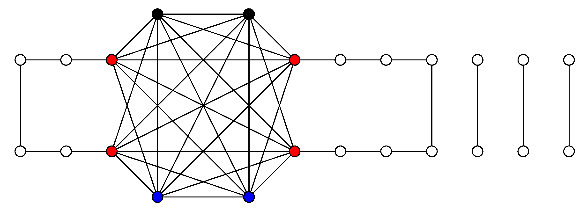
Figure 3.
The strong resolving graph of the graph illustrated in Figure 2.
Figure 3.
The strong resolving graph of the graph illustrated in Figure 2.

Figure 4.
A chain of cycles containing six cycles and two cycles .

Figure 5.
The strong resolving graph of the graph illustrated in Figure 4.
Figure 5.
The strong resolving graph of the graph illustrated in Figure 4.

© 2020 by the author. Licensee MDPI, Basel, Switzerland. This article is an open access article distributed under the terms and conditions of the Creative Commons Attribution (CC BY) license (http://creativecommons.org/licenses/by/4.0/).
Share and Cite
MDPI and ACS Style
Kuziak, D. The Strong Resolving Graph and the Strong Metric Dimension of Cactus Graphs. Mathematics 2020, 8, 1266. https://doi.org/10.3390/math8081266
AMA Style
Kuziak D. The Strong Resolving Graph and the Strong Metric Dimension of Cactus Graphs. Mathematics. 2020; 8(8):1266. https://doi.org/10.3390/math8081266
Chicago/Turabian StyleKuziak, Dorota. 2020. "The Strong Resolving Graph and the Strong Metric Dimension of Cactus Graphs" Mathematics 8, no. 8: 1266. https://doi.org/10.3390/math8081266
Note that from the first issue of 2016, this journal uses article numbers instead of page numbers. See further details here.