A Robust Algorithm for Classification and Diagnosis of Brain Disease Using Local Linear Approximation and Generalized Autoregressive Conditional Heteroscedasticity Model

Abstract

Regions detection has an influence on the better treatment of brain tumors. Existing algorithms in the early detection of tumors are difficult to diagnose reliably. In this paper, we introduced a new robust algorithm using three methods for the classification of brain disease. The first method is Wavelet-Generalized Autoregressive Conditional Heteroscedasticity-K-Nearest Neighbor (W-GARCH-KNN). The Two-Dimensional Discrete Wavelet (2D-DWT) is utilized as the input images. The sub-banded wavelet coefficients are modeled using the GARCH model. The features of the GARCH model are considered as the main property vector. The second method is the Developed Wavelet-GARCH-KNN (D-WGK), which solves the incompatibility of the WGK method for the use of a low pass sub-band. The third method is the Wavelet Local Linear Approximation (LLA)-KNN, which we used for modeling the wavelet sub-bands. The extracted features were applied separately to determine the normal image or brain tumor based on classification methods. The classification was performed for the diagnosis of tumor types. The empirical results showed that the proposed algorithm obtained a high rate of classification and better practices than recently introduced algorithms while requiring a smaller number of classification features. According to the results, the Low-Low sub-bands are not adopted with the GARCH model; therefore, with the use of homomorphic filtering, this limitation is overcome. The results showed that the presented Local Linear (LL) method was better than the GARCH model for modeling wavelet sub-bands.

1. Introduction

Electromagnetic imaging techniques provide valuable information about the human body. One of these methods is the Magnetic Resonance Imaging (MRI) of the brain [1]. One major area of research that has expanded in medical engineering involves diagnostic tools by machine control for a quicker and easier inference, which can be a great help for physicians in clinical medicine. Therefore, in recent years, mathematical methods have attracted much attention to the analysis of neural network data [2]. Brain images are considered as interesting subjects in the mathematical application and diagnosis of brain disorders in a patient [3]. The MRI can be used to examine the status of the brain tissue and discover whether or not there is a disease [4]. In MRI imaging, the patient is exposed to a strong magnetic field, after which radio waves are leaked toward him. The body’s tissues emit another radio wave in response to this position. By receiving these radio waves emitted from the patient’s body and by analyzing these waves via a powerful computer, images are created on the device monitor that show the levels of the target organ parts. The next step involves extracting features.

The Two-Dimensional Wavelet Transform (DWT) and the Principal Component Analysis (PCA) were the methods that were used to extract the features of the images [5,6]. Then, the classification methods were used to diagnosis the disease type in the brain [7,8]. Chaplot, et al. [9] used two-dimensional DWT sub-bands to extract the features in their research on Alzheimer’s Disease (AD). Additionally, Daubechies filters were used as a filtering technique. The outcome illustrated that the Support Vector Machine (SVM) with radial base function and the polynomial kernel has a higher performance than linear neural networks and SVM [10,11]. Hackmack, et al. [12] used multidimensional complex wavelet transformations, and then linear SVM, to determine multi-scale brain images. The results showed that low-band scales include more information than high-frequency values. Maitra and Chatterjee [13] presented a Slantlet deformation—developed DWT—to extract the containing features of the brain’s images. The Fuzzy C-Meaning (FCM) method has been used to analyze the brain MRI, based on the characteristics of the image histogram, in order to determine a healthy subject from Alzheimer’s disease. Ramathilagam, et al. [14] used the c-means fuzzy modified algorithm to divide the brain MRI image with a T1-T2 weight. Since the c-means standard factor is intensively sensitive to the noise-induced area during extraction, the authors proposed to repeat the dist-max algorithm before executing the method.

Rivest-Hénault and Cheriet [15] used a local linear representation to model the brain tissue, after which regional models were embedded in the framework of the surface set in order to control the spatial integrity of division. Hussain, et al. [16] classified the images as normal or abnormal using (Back-Propagation Neural Networks) BPNN feed-forward, with characteristics derived from dynamic statistics and 2D-DWT. Bhattacharyya and Kim [17] presented an image segmentation technique for detecting a tumor with MRI images. The existing thresholding techniques produced different results in each image. Therefore, in order to achieve a satisfactory result in the brain tumor image, they presented a methodology that found the tumor to be unique. Kim, et al. [18] studied the diagnosis of Alzheimer’s disease based on the Electroencephalogram (EEG) signal of the brain using genetic algorithms and neural networks. One of the remarkable points in this study was the ability to differentiate Alzheimer’s patients from the mild stage of healthy subjects with 82% accuracy using a single-channel EEG signal [19]. Additionally, in another study, the comparison of the EEG signaling disorder of healthy people with that of brain tumor patients was calculated by entropy. According to the results, in low-frequency patients, low-rhythms of EEG signals such as Delta and Theta bands have a higher power spectrum than for healthy people. Gholipour, et al. [20] described the use of a completely new automated software algorithm using the standard MRI sequence before and after Contra T1. The T1 weighs in before and after Contra, and the images are automatically interconnected and normalized. The volume of tumor growth is automatically calculated. In their study, they were able to test a method for calculating the size of the tumor when it was enlarged by the collapse of the cavity and, of course, when the enlarged tumor was covered with semi-autogenous blood in a cutaneous cavity. It detected an increase in tumor volume among blood products, which rarely reduced measurements when using other techniques. Their approach seems to overcome many challenges by assessing the response to increased brain tumors and leading to more validation. Zacharaki, et al. [21] studied machine-learning algorithms that automatically identify the relevant features and are desirable for brain tumor differentiation. They studied various machine-learning techniques for classifying the brain tumor based on the features extracted from conventional MRI and perfusion. Their study was performed by mutual validation of Leave-One-Out (LOO) exodus on 101 brain tumors, obtained using a pack evaluation in combination with the best first-order algorithm and K-Nearest Neighbour (KNN) algorithm classification, reaching 96.9%. When differentiated, it became Glimatic and 94.5% when distinguished from a low-grade neoplasm. Fritzsche, et al. [22] completed a study of 15 patients with brain tumors and 18 patients with Mild Cognitive Impairment (MCI); eight remained stable in a three-year follow-up, and 15 were healthy individuals. The classification was also improved by limiting the analysis to the left-brain hemisphere. Devanand, et al. [23], using morphometric mapping of MRI, evaluated the local changes of the hippocampus grains and entorhinal cortex in predicting the transformation from a MCI cognitive impairment to an AD brain tumor. In the MCI model, Cox regression models for the conversion time to conversion converters were made for AD (n = 31) and 99 non-converted controls for age, sex, and education. In Zöllner, et al. [24], the performances of reduction features such as the Pearson correlation coefficient, principal components analysis, and independent component analysis in the classification of Glioma’s disease were analyzed using a backup vector machine classifier.

Afshar, et al. [25] studied classification using CapsNets for the detection of brain tumors in order to present a developed architecture with higher accuracy. Their findings indicated that the presented method could overcome Convolutional Neural Networks (CNNs) successfully. Mohan and Subashini [26] provided a clinical study of brain tumor imaging related to gliomas. They used related methods of segmentation and classification. Huang, et al. [27] proposed an algorithm based on the rough set method. They presented a hybrid method with the use of FCM. Initially, the feature table was set based on FCM clustering amounts. Then, the relationship among features showed similarity criteria in each cluster.

In this paper, we presented three algorithms, named WGK, D-WGK, and WLK. The first presented method is Wavelet-GARCH-KNN (WGK). In this method, we first used a two-stage 2D-DWT to decompose the input images into sub-bands of wavelets. The reached wavelet coefficients were features of classification. Then, the GARCH model was used for feature extraction with the use of HH1, HL1, LH1, and second stage HH2, HL2, LH2. Because of the incompatibility of Local Linear (LL) with the GARCH model, this sub-band was ignored [28]. To reduce the number of features, the PCA and PCA + LDA method was then used with the extracted feature brain lesion being classified via KNN methods. The results are illustrated in the results section. The second presented method is named Developed Wavelet-GARCH-KNN (D-WGK). In the second method, we overcame the limitation of the WGK algorithm using homomorphic filtering before a wavelet transformation. Therefore, the LL2 sub-band participated in the GARCH model. Then, similarly to the WGK method, the KNN method was designated for the classification of brain tumors. The third method was Wavelet-LLA-KNN (WLK). In this method, all sub-bands of the wavelet decomposition were used for modeling with the LLA algorithm. The remaining part of the third method was also similar to the WGK and D-WGK method.

2. Methods and Materials

2.1. Image Processing

The modern world of today allows digital images to be analyzed and stored [29]. To get better results, it is sometimes necessary to make changes to these images. These changes have three main purposes: processing, analysis, and image perception. For this reason, computer image processing systems have been developed to perform these operations with better speed and accuracy. In these systems, four major processes occur pre-processing, image quality enhancement, image transformation, and classification and segmentation. In these methods, using mathematical science, rules have been created by computers to simulate human visual elements, and this is an aspect of image analysis that is used for specific purposes. Computer Vision is the analysis of scientific images in various scientific branches such as medicine, engineering, molecular imaging, astronautics, security, etc. Modern digital technology has made it possible to manipulate multidimensional signals from systems ranging from simple digital circuits to multiple parallel computers [30,31].

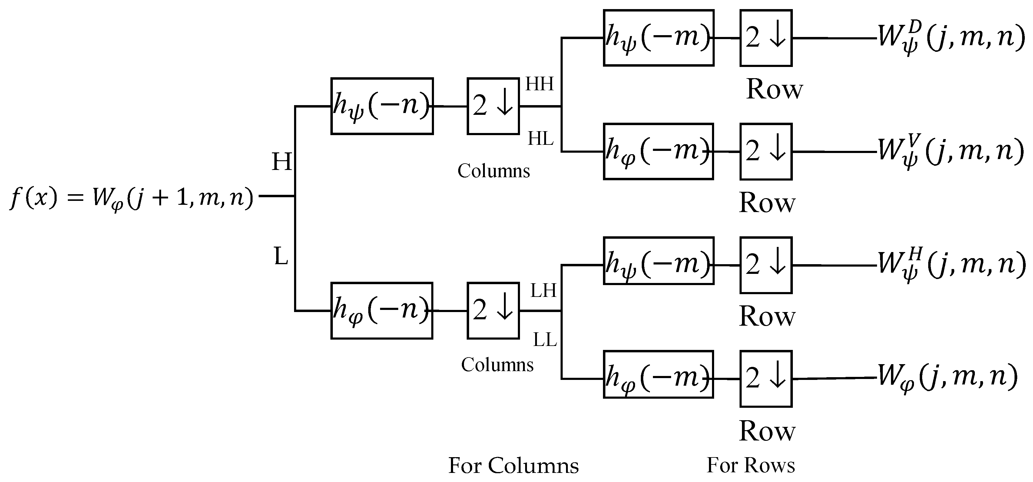
2.2. Discrete Wavelet Transform (DWT)

Let $f\left(x\right)\in L^2\left(\mathit{R}\right)$ be the function wavelet expansion related to the wavelet $\psi \left(x\right)$ and scaling $\phi \left(x\right)$ function [20]; we then have:

$$f\left(x\right)=\frac{1}{\sqrt{M}}{\displaystyle \sum }_k{W}_{\phi }\left(j_0,k\right){\varphi }_{j_0,k}\left(x\right)+\frac{1}{\sqrt{M}}{\displaystyle \sum }_{j=j_0}^J{\displaystyle \sum }_k{W}_{\psi }\left(j,k\right){\psi }_{j,k}\left(x\right)$$

(1)

$$W_{\phi }\left(j_0,k\right)=\frac{1}{\sqrt{M}}{\displaystyle \sum }_{x=0}^{M-1}f\left(x\right){\varphi }_{j0 ,k}\left(x\right)$$

(2)

$$W_{\psi }\left(j,k\right)=\frac{1}{\sqrt{M}}{\displaystyle \sum }_{x=0}^{M-1}f\left(x\right){\psi }_{j,k}\left(x\right) j\ge j_0$$

(3)

$${\varphi }_{j,k}\left(x\right)=2^{\frac{j}{2}}\varphi \left(2^{j}x-k\right)$$

(4)

$${\psi }_{j,k}\left(x\right)=2^{\frac{j}{2}}\psi \left(2^{j}x-k\right)$$

(5)

where $f\left(x\right)$ is the input variable as a vector, and ${\phi }_{j_0,k}\left(x\right)$ and ${\psi }_{j,k}\left(x\right)$ are the scaling coefficient and wavelet coefficient, respectively. x = 0, 1, …, M − 1, j = 0, 1, …, J − 1, k = 0, 1, 2, ..., M − 1, where M is the number of samples to be transformed that is equal to $2^J$, $J$ is the number of transformation levels, and $j_0$ is a random starting scale. The expansion function is a series of crisp numbers; it is also called the discrete wavelet transform of $f\left(x\right)$. The representation of the discrete function of $f\left(x\right)$ can be written as a weighted summation of wavelet ${\psi }_{j,k}\left(x\right)$ and the scaling coefficient ${\phi }_{j_0,k}\left(x\right)$, as shown in Equation (1). In this equation, $W_{\varphi }\left(j_0,k\right)$ and $W_{\psi }\left(j_0,k\right)$ are the approximation coefficient and detail coefficient, respectively. The expansion coefficients are shown as follows.

Figure 1 shows a two-step wavelet transformation that generates four sub-bands, where ${\psi }^H$, ${\psi }^V$ and ${\psi }^{D }$ indicate deviations along the horizontal, vertical, and diagonals edges, respectively. In this diagram, 2 ↓ shows a down stampeding indicator. 2D-DWT can be executed with digital filtration and down samplers. The other sub-bands are generated with discrete 2D scaling functions, with the use of 1D-FWT on f(x, y) [32]. For the computation of the DWT coefficients, we should consider the multiresolution refinement equation, as shown in Equations (6) and (7):

$${\varphi }_{j,k}\left(x\right)={\displaystyle \sum }_n{2}^{\frac{j}{2}}\varphi \left(2^{j}x-n\right).h_{\varphi }\left(n\right)$$

(6)

$${\psi }_{j,k}\left(x\right)={\displaystyle \sum }_n{2}^{\frac{j}{2}}\psi \left(2^{j}x-n\right).h_{\psi }\left(n\right)$$

(7)

where $h_{\varphi }$ and $h_{\psi }$ are the scaling vector and wavelet vector, respectively. $h_{\varphi }$ and $h_{\psi }$ may be considered as weights for the summation of Equations (6) and (7). With the inclusion of Equations (6) and (7) into Equations (2) and (3), the following questions result.

$$W_{\varphi }\left(j,k\right)=h_{\varphi }\left(-n\right)W_{\varphi }\left(j+1,n\right), \left(n=2k, k\ge 0\right)$$

(8)

$$W_{\psi }\left(j,k\right)=h_{\psi }\left(-n\right)W_{\psi }\left(j+1,n\right) j\ge j_0$$

(9)

The scaling and wavelet coefficient of a certain scale $j$ may be obtained via the convolution of the scaling coefficients of the next scale $j+1$ (with finer detail) with the order-reversed scaling and wavelet vectors $h_{\varphi }\left(-n\right)$ and $h_{\psi }\left(-n\right)$. Based on Figure 1, the results of the first level of transformation for the column of an input image are as follows:

$$\begin{array}{cc}{W}_{\varphi }\left(j+1,m,n\right)& =h_{\varphi }\left(-n\right)\ast \left(h_{\varphi }\left(-m\right)\ast W_{\varphi }^{2\uparrow }\left(j,m\right)+h_{\psi }\left(-m\right)\ast W_{\psi }^{2\uparrow }\left(j,m\right)\right)\hfill \\ & +h_{\psi }\left(-n\right)\ast \left(h_{\varphi }\left(-m\right)\ast W_{\varphi }^{2\uparrow }\left(j,m\right)+h_{\psi }\left(-m\right)\ast W_{\psi }^{2\uparrow }\left(j,m\right)\right), (k\hfill \\ & \ge 0)\hfill \end{array}$$

(10)

$$\begin{array}{cc}{W}_{\varphi }\left(j+1,m,n\right)& =h_{\varphi }\left(-n\right)h_{\varphi }\left(-m\right)\ast W_{\varphi }^{2\uparrow }\left(j,m\right)+h_{\varphi }\left(-n\right)h_{\psi }\left(-m\right)\ast W_{\psi }^{2\uparrow }\left(j,m\right)\hfill \\ & +h_{\psi }\left(-n\right)h_{\varphi }\left(-m\right)\ast W_{\varphi }^{2\uparrow }\left(j,m\right)+h_{\psi }\left(-n\right)h_{\psi }\left(-m\right)\ast W_{\psi }^{2\uparrow }\left(j,m\right), (k\hfill \\ & \ge 0)\hfill \end{array}$$

(11)

$$\begin{array}{cc}{W}_{\varphi }\left(j+1,m,n\right)& =h_{\varphi }\left(-n\right)h_{\varphi }\left(-m\right)\ast W_{\varphi }^{2\uparrow }\left(j,m\right)+h_{\varphi }\left(-n\right)h_{\psi }\left(-m\right)\ast W_{\psi }^{2\uparrow }\left(j,m\right)\hfill \\ & +h_{\psi }\left(-n\right)h_{\varphi }\left(-m\right)\ast W_{\varphi }^{2\uparrow }\left(j,m\right)+h_{\psi }\left(-n\right)h_{\psi }\left(-m\right)\ast W_{\psi }^{2\uparrow }\left(j,m\right), (k\hfill \\ & \ge 0)\hfill \end{array}$$

(12)

Generally, 2D- $\phi \left(x,y\right)$, and 3D- ${\psi }^H\left(x,y\right)$, ${\psi }^V\left(x,y\right)$, and ${\psi }^D\left(x,y\right)$ are required to generate a 1D scaling function φ and related wavelet ψ [20].

$$\varphi \left(x,y\right)=\varphi \left(x\right)\varphi \left(y\right)$$

(13)

$${\psi }^H\left(x,y\right)=\psi \left(x\right)\varphi \left(y\right)$$

(14)

$${\psi }^V\left(x,y\right)=\varphi \left(y\right)\varphi \left(x\right)$$

(15)

$${\psi }^D\left(x,y\right)=\psi \left(x\right)\psi \left(y\right)$$

(16)

2.3. Generalized Autoregressive Conditional Heteroscedasticity

Bollerslev was the first researcher who developed the GARCH method [33]. It can be considered as being the variance of the time variable, for example, an oscillation. Conditional requires immediate dependence on past observations, and self-control combines past data at the present time. GARCH models are statistical methods that are more common in the economy. Engle [34] presented the process of Autoregressive Conditional Heteroscedasticity (ARCH) to change the conditional variance over time as a factor of past mistakes that remain based on the conditional constant variance. The GARCH process (Algorithm 1) is a general form of ARCH and is a time series modeling technique that uses the last variance to predict future variances.

Algorithm 1. GARCH

1: Input: $y_t,P,Q,dist$ 2: Output: $a_i, {ϵ}_t$ 3: Step 1: Estimate AR(q): 4: $y_t=a_0+a_1{y}_{t-1}+\cdots .+a_q{y}_{t-q}+{ϵ}_t$ 5: ${\widehat{ϵ}}_t^2={\widehat{a}}_0+{{\displaystyle \sum }}_{i=1}^q\widehat{a_i}{\widehat{ϵ}}_{t-i}^2$ 6: Step 2: Compute and plot the autocorrelations of ${ϵ}^2$ by: 7: $\rho =\frac{{{\displaystyle \sum }}_{t=i+1}^T\left({\widehat{ϵ}}_t^2-{\widehat{\sigma }}_t^2\right)\left({\widehat{ϵ}}_{t-1}^2-{\widehat{\sigma }}_{t-1}^2\right)}{{{\displaystyle \sum }}_{t=1}^T{\left({\widehat{ϵ}}_t^2-{\widehat{\sigma }}_t^2\right)}^2}$ 8: Step 3: null hypothesis states that there are no ARCH or GARCH errors

2.4. Local Linear Approximation

The Local Linear Approximation is calculated via [35]. In this method, the first and second derivatives are determined so as to generate a fitting function with the observation data.

Let x have three value x(1), x(2), and x(3). An LLA for the derivative of x at the x(2) is calculated via the mean of the two slopes between x(1)−x(2) and between x(2)−x(3), which can now be calculated from x(3) and stored in the matrix y of the same order as x(3) where the kth row of y is:

$$y_{k1}=x_{k2},$$

(17)

$$y_{k2}=\frac{x_{k3}-x_{k1}}{2\tau \mathsf{\Delta }t},$$

(18)

$$y_{k3}=\frac{x_{k1}-2x_{k2}+x_{k3}}{{(\tau \mathsf{\Delta }t)}^2}.$$

(19)

$$\frac{dx\left(1-\tau \right)}{dt}\approx \frac{x\left(1+2\tau \right)-x\left(1\right)}{2\tau \mathsf{\Delta }t}$$

(20)

where the first column of y is the value of x at the moment of measurement indexed in the second column of x(3), and the second and third columns of y are the approximated first and second derivatives, respectively, at that same moment of measurement. In this case, τ = 1 since x(1), x(2), and x(3) are successive measures, and ∆t is the time interval among the measures. The others (for instance x(1), x(3), and x(5)) can be calculated with τ = 2 being substituted into Equation (20).

2.5. K-Nearest Neighbour Algorithm

KNN is a simple form of machine learning [31,36]. In this algorithm, an article is classified by the values of its neighbors, which are allocated to k ($\in {\mathbb{N}}^{+}$) nearest neighbors [37]. The similarity of each object in a class is utilized as the weight of the class. In the case of a few of the k nearest neighbors sharing a category, the per-neighbor weights of that category are included together at that point, and the obtained weighted entirety is utilized as the probability score of the candidate categories. A positioned list is obtained for the test archive. By thresholding these scores, twofold category assignments are obtained.

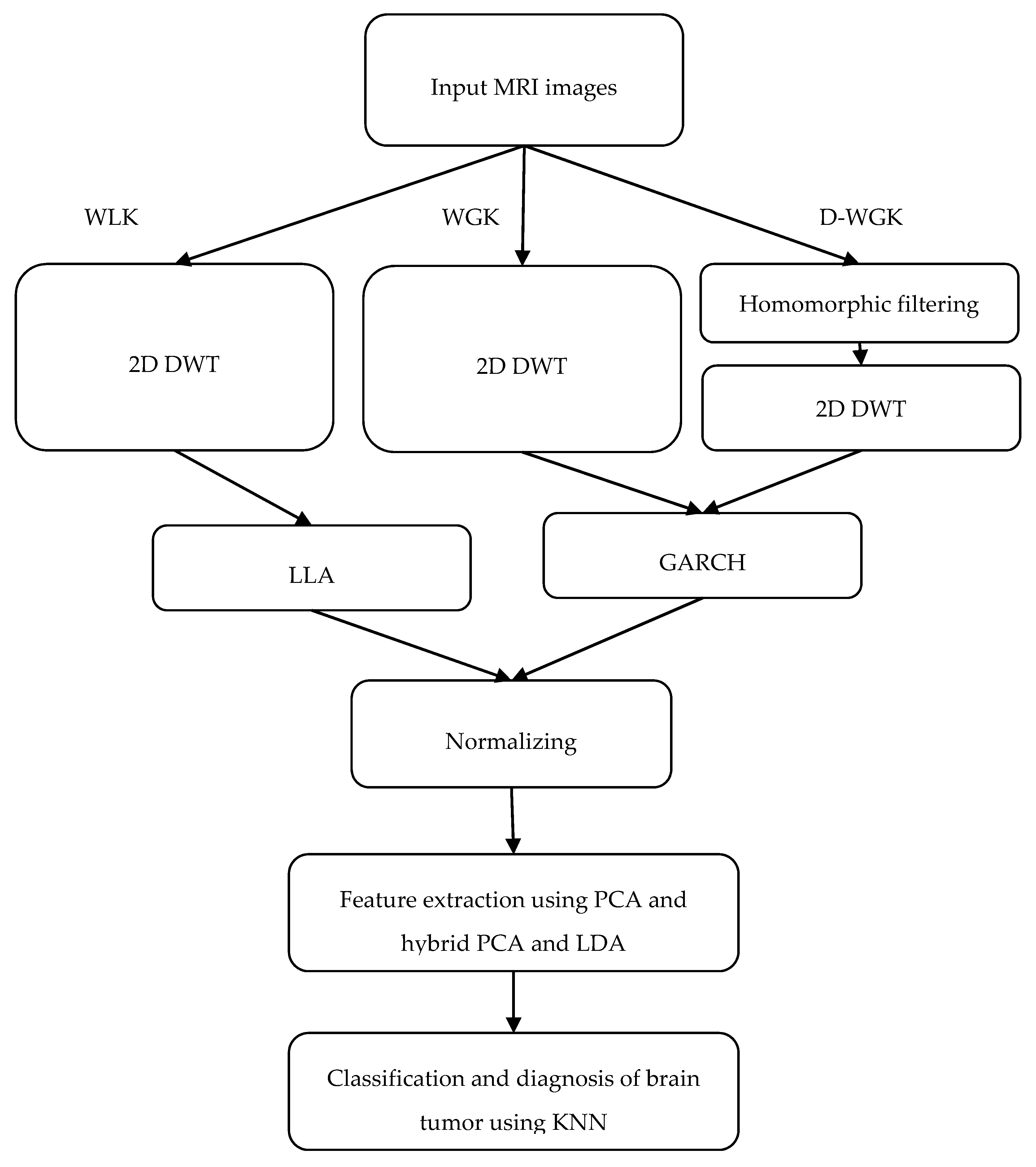
2.6. Proposed Method

In this paper, we aim to use mathematical methods to diagnose brain diseases. We implemented three methods for the classification and diagnosis of brain tumors (Algorithm 2). The first presented method is Wavelet-GARCH-KNN (WGK). In this method, we first used two-stage 2D-DWT to decompose input images into sub-bands of wavelets. The obtained wavelet coefficients are features of classification. Then, the GARCH model was used for feature extraction with the use of HH1, HL1, LH1, and second-stage HH2, HL2, LH2. Because of the incompatibility of LL with the GARCH model, this sub-band was ignored. To reduce the number of features, the PCA and PCA + LDA method was then used, with extracted feature brain lesions being classified with the use of KNN methods. The results are illustrated in the results section.

The second presented method is named Developed Wavelet-GARCH-KNN (D-WGK). In the second method, we overcame the limitation of the WGK algorithm by using homomorphic filtering before a wavelet transformation. Therefore, the LL2 sub-band participated in the GARCH model. Then, similarly to the WGK method, the KNN method was designated for the classification of brain tumors.

The third method is Wavelet-LLA-KNN (WLK). In this method, all sub-bands of wavelet decomposition were used for modeling with the LLA algorithm. The remaining part of the third method was also similar to the WGK and D-WGK method. The results of each algorithm are depicted in the below sections. The structure and proposed model in this study are shown in Figure 2.

Algorithm 2. Presented

1: Input:$y_{m\times m}=\left\{m\times m\right\}\in R^2$ 2: Switch: 3: Case 1: WGK 4: Step 1: Wavelet decomposition for all images 5: Step 2: Calculate GARCH parameters for sub-bands of high-frequency detail of (HH1, HL1, LH1, HL2, LH2) 6: Step 3: Normalization of features 7: Step 4: Feature reduction using PCA and PCA+LDA 8: Step 5: Classification of Features using KNN 9: Case 2: D-WGK 10: Step 1: Apply homomorphic filtering for all images 11: Step 2: Wavelet decomposition for all images 12: Step 2: Calculate GARCH parameters for all sub-bands of high-frequency detail of (HH1, HL1, LH1, HL2, LH2, LL2) 13: Step 3: Normalization of features 14: Step 4: Feature reduction using PCA and PCA+LDA 15: Step 5: Classification of Features using KNN 16: Case 3: WLK 17: Step 1: Wavelet decomposition for all images 18: Step 2: Calculate LLA parameters 19: Step 3: Normalization of features 20: Step 4: Feature reduction using PCA and PCA+LDA 21: Step 5: Classification of Features using KNN 22: Comparison and analysis

3. Results and Discussion

3.1. Datasets

In this paper, we used seven brain diseases to implement and test the presented methods. They consist of Alzheimer’s, Alzheimer plus visual agnosia, Glioma, Huntington, Meningioma, Pick, and Sarcoma. These diseases, in conjunction with normal brain images, include 240 MRI images from the Harvard medical school website. All images are from T2-weighted MR brain images in the axial plane and have 256 × 256 pixels. These images were saved in different folders and studied separately. Therefore, after feature extraction, they were aggregated into a single code folder.

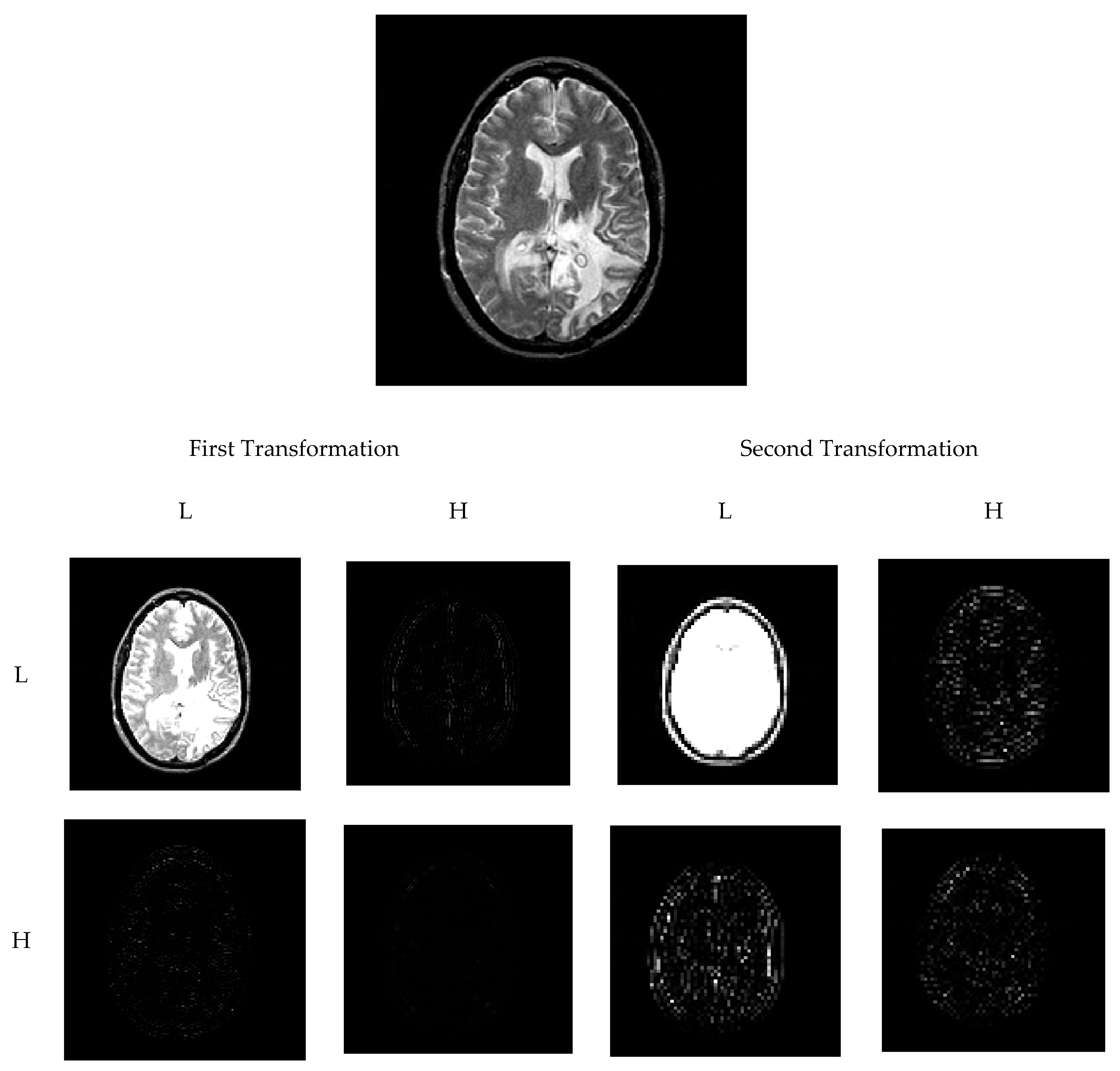
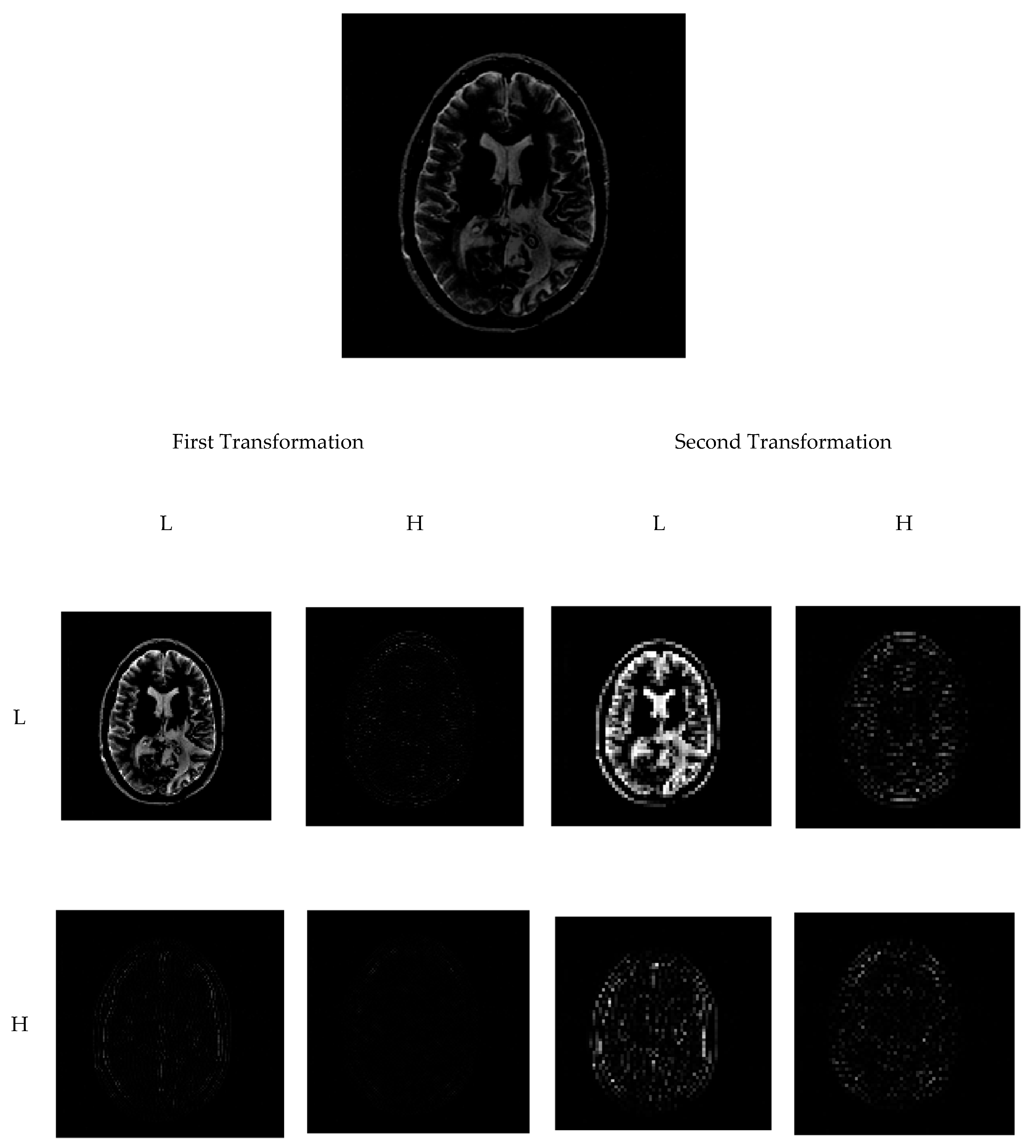
3.2. Two-dimensional Discrete Wavelet Transforms (2D-DWT)

In this paper, we used 2D-DWT to separate the sub-bands of images. In this transformation, we input images from 256 × 256 pixels to 131 × 131 first-stage sub-bands and 69 × 69 sub-bands. The example of a wavelet transformation is shown in Figure 3. Additionally, for the second aforementioned method, we needed homomorphic filtering.

The results of the wavelet discretization when using homomorphic filtering ($\sigma =5$) are shown in Figure 4. The top images show the original image without (with) the filtration, and the first and second transformation are shown on the left and right sides of the images, respectively. Regarding the literature studies, the GARCH model was not compatible with LL2 sub-bands [38]. This situation is obviously shown in Figure 3 (LL2). Because all the brain sections of the images were almost within the GARCH model in (1, 1), we did not find the model coefficient to be significant for the GARCH (1, 1) model. In this paper, we overcame this limitation and made the LL2 model be compatible with the GARCH (1, 1) model. To overcome this condition, we used homomorphic filtration for the main image, and then the 2D-DWT was performed on it. With this method, we increased the contrast of the LL2 sub-band, as can be seen in Figure 4 (LL2).

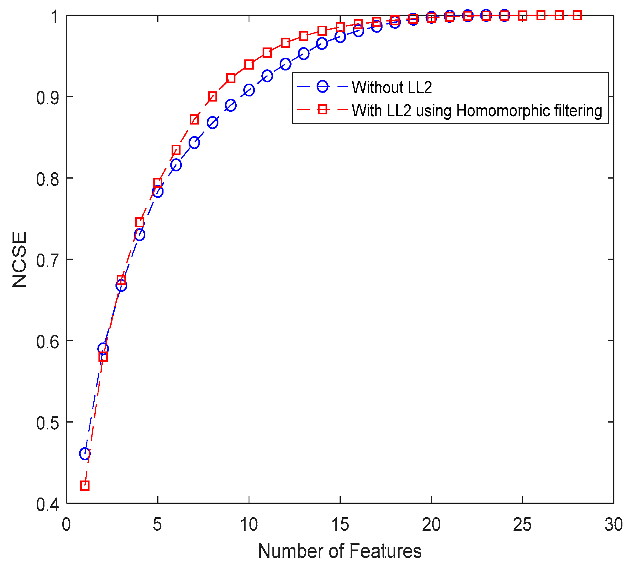
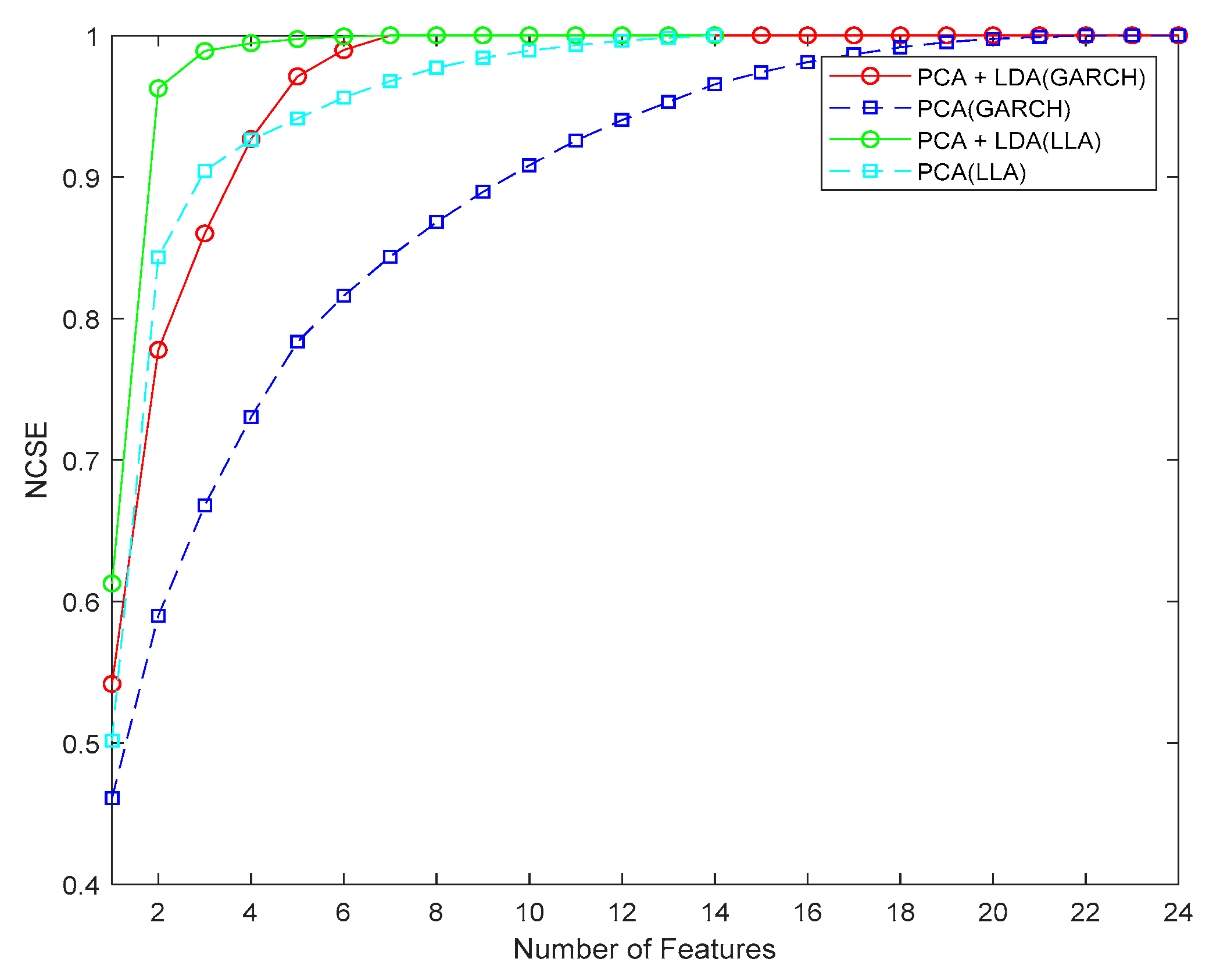
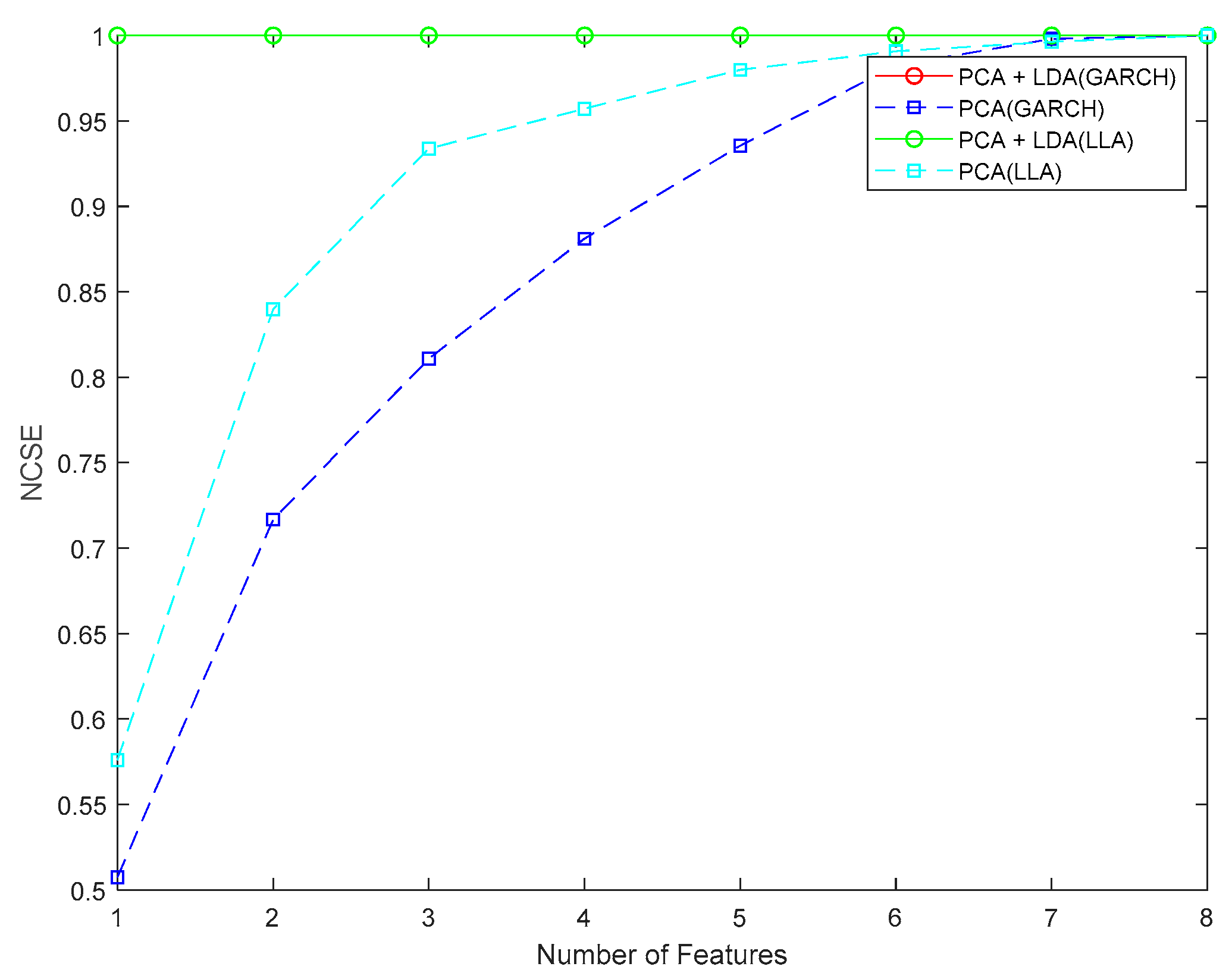
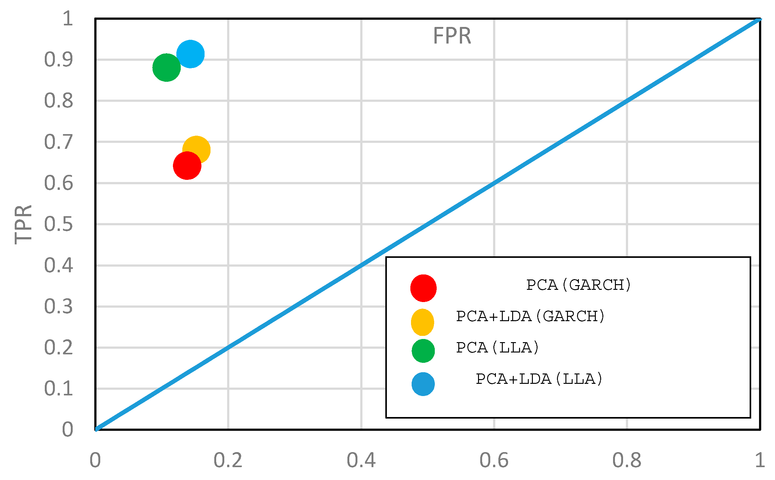
3.3. Feature Reduction

In this section, we used nonconvulsive status epilepticus (NCSE) to extract features and classify them. Via this method, we can classify the features into two classification states: two-classes and eight-classes. In the two-class state, we classify the features into two classes to diagnosis the normal and abnormal MRI images. Using this state, we can find patient and inpatient brain images. Moreover, using the eight-class state, we can classify the brain images into seven different classes in conjunction with normal brain images.

In this paper, we studied different methods to reduce features, consisting of:

• WGK: Using GARCH without LL2 + PCA
• WGK: Using GARCH without LL2 + PCA + LDA
• D-WGK: Using Homomorphic filtering + GARCH with LL2 + PCA
• WLK: Using LLA + PCA
• WLK: Using LLA + PCA + LDA

The results are depicted in Figure 5, Figure 6, Figure 7 and Figure 8. Figure 5 shows the feature reduction plots used to find the best number of classes. In this figure, we used two methods, 2D-DWT and GARCH (1, 1), used with and without LL2 sub-bands. The result shows that with the addition of LL2 to the GARCH method, the model is developed. Furthermore, the results of the PCA method show that we can use 14 features for the classification of images.

Furthermore, this enhancement is shown in Figure 6 for the two-class state. Additionally, in this state, the method is developed, and a number of features are decremented from 6 to 5. This can speed up the classification method and increase the accuracy of the methods because we used all sub-bands of the 2D-DWT method for classification with fewer features.

Figure 7 and Figure 8 show the feature reduction results for the presented LLA and GARCH model using the PCA and PCA + LDA methods. In the eight-class method (Figure 7), the best number of features for the GARCH and PCA method was 20, which for GARCH + PCA + LLDA decreased to 10 features. Using the presented method, the LLA + PCA method’s number of features decreased to 7 features. Furthermore, for the LLA + PCA + LDA method, the best number of features should be three features. The results showed that the last presented method decreased the number of features to 3 so that it would be great for feature reduction.

For a two-class state (Figure 8), this reduction is conspicuously shown. The resolution between the classes is high, which indicates the ability of LLA + PCA + LDA in incremental inter-class distances and decremental intra-class distances.

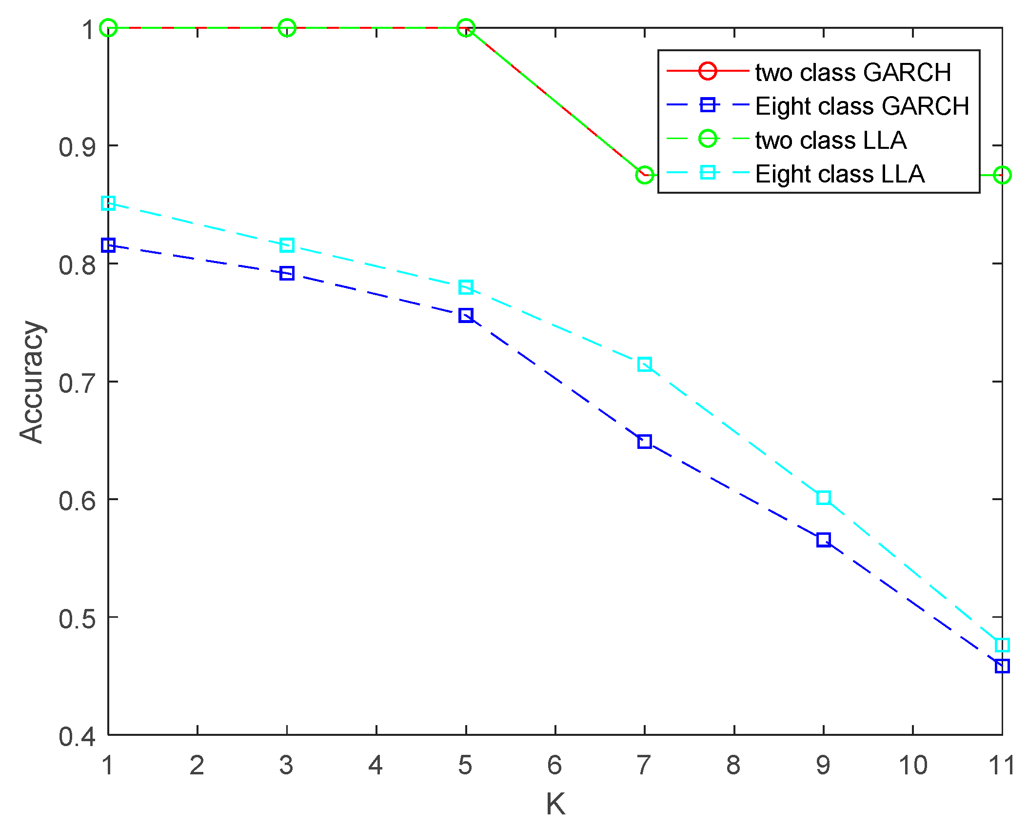
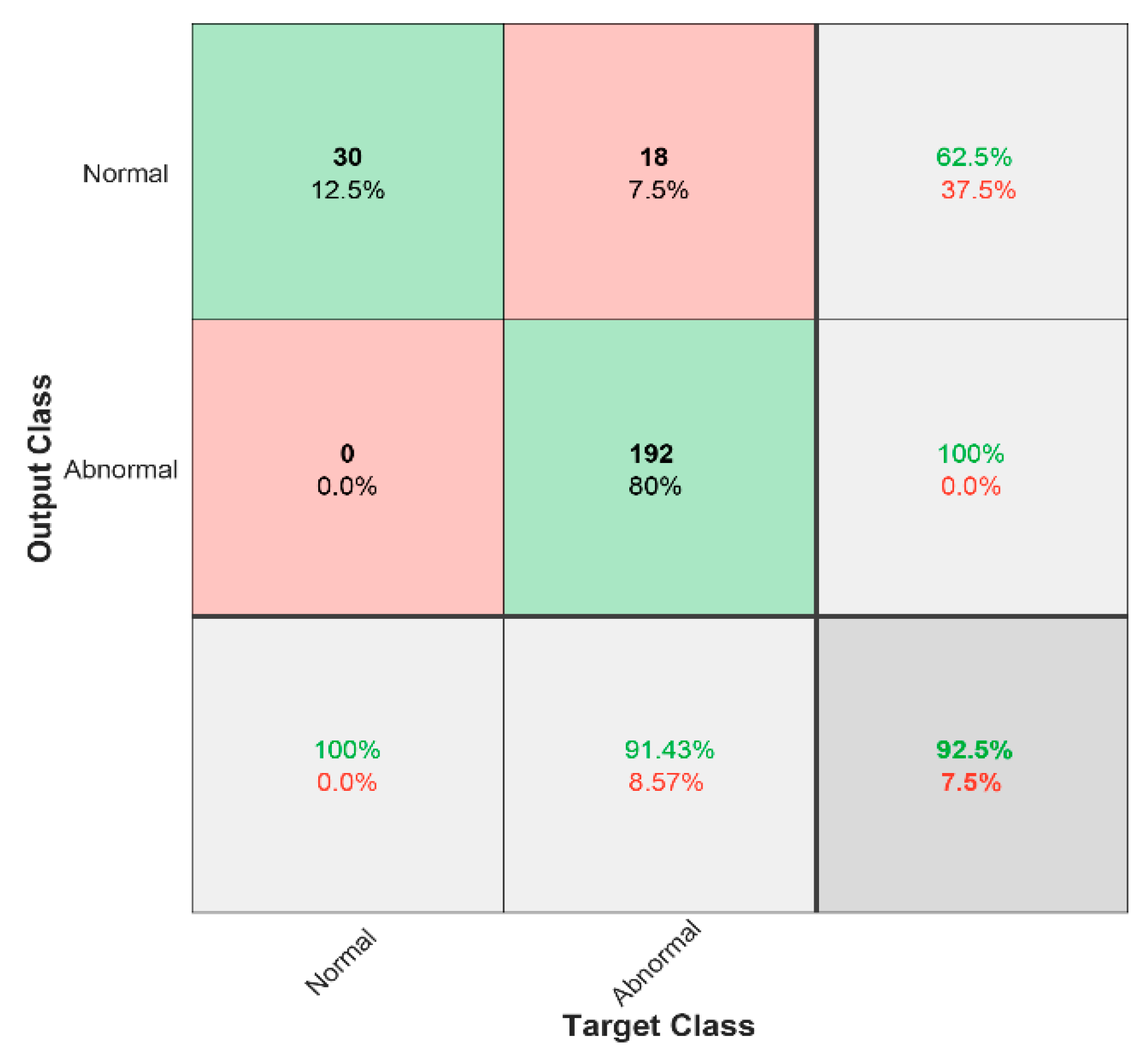
3.4. The Classification Results

In this paper, we used the k-Nearest Neighborhood (KNN) method to classify the input features. KNN is a non-parametric method used in data mining, machine learning, and pattern recognition. The KNN algorithm is one of the ten most used algorithms in various machine learning and data mining projects in the industry. The KNN algorithm can be used for classification and regression issues. However, it is often used for classification issues.

The value of K in the KNN method is one of the effective parameters in classification. The mean classification accuracy was determined for different values of K, which was increased from 1 to 11 in steps of two for both states. The results are depicted in Figure 9. The results show that, for K ≤ 5, the classifier has good efficiency. Furthermore, the accuracy of the LLA method in the KNN classifier is greater than the GARCH method.

In the statistics, indicators of sensitivity and specificity are utilized to evaluate the result of the binary classification (two-class). When the data can be divided into positive and negative groups, the accuracy of the results of a test that divides the information into these two categories is measurable and describable using sensitivity and attribute indicators. Sensitivity means a proportion of positive cases that will test them correctly as being positive. Specificity means the proportion of negative cases that mark them correctly as being negative.

True Positive (TP): The disease is diagnosed correctly.

False Positive (FP): A healthy person is diagnosed with mistakes.

True Negative (TN): A healthy person is diagnosed correctly.

False Negative (FN): The disease is diagnosed with mistakes.

The sensitivity parameter is calculated by dividing the numbers of TP cases by the sum of TP cases and FN cases.

$$sensitivity, \mathrm{TPR}=\frac{\mathrm{TP}}{\mathrm{TP}+\mathrm{FN}}$$

(21)

In a similar way, the specificity results are the division of TN cases by the sum of FP and TN cases.

$$specificity,\mathrm{TNR}=\frac{\mathrm{TN}}{\mathrm{TN}+\mathrm{FP}}$$

(22)

Other classification criteria, such as precision, accuracy, and fall-out, are defined as following Equations (23)–(25).

$$precision,\mathrm{PPV}=\frac{\mathrm{TP}}{\mathrm{TP}+\mathrm{FP}}$$

(23)

$$accuracy\left(\mathrm{ACC}\right)=\frac{\mathrm{TP}+\mathrm{TN}}{\mathrm{TP}+\mathrm{TN}+\mathrm{FP}+\mathrm{FN}}$$

(24)

$$fall-out\left(\mathrm{FPR}\right)=\frac{\mathrm{FP}}{\mathrm{FP}+\mathrm{FN}}$$

(25)

The results of the classification using the LLA method are shown in

Table 1. The comparison between the presented methods.

Method	Class	Images	Features	Accuracy
Ref. *	6	56	6	91.5
PCA + LDA (WGK) **	8	80	10	89.4
PCA (WGK) **	8	80	22	90.1
Proposed PCA + LDA (D-WGK)	8	240	10	90.2
Proposed PCA (D-WGK)	8	240	20	89.3
Proposed PCA + LDA (WLK)	8	240	3	92.5
Proposed PCA (WLK)	8	240	7	91.3

* Marti nez, et al. [39]; ** Kalbkhani, Shayesteh and Zali-Vargahan [38].

and

Table 2. The results of the classification for eight-class states using PCA + LDA (WLK).

Diseases	TPR	TNR	PPV	ACC	FPR
Alzheimer	0.933	1	0.903	0.967	0
Alzheimer+	0.933	1	0.875	0.967	0
Glioma	0.900	1	1	0.950	0
Huntington	0.967	1	0.906	0.983	0
Meningioma	0.967	1	1	0.983	0
Pick	0.867	1	0.839	0.933	0
Sarcoma	0.833	1	0.926	0.917	0

. Table 1 shows the results of the classification using the presented methods. The results show that the maximum accuracy belongs to the presented LLA method that conducted the extraction using the combination of the PCA and LDA methods. Moreover, the minimum one belongs to the GARCH method that used the PCA feature extraction method.

Therefore, we can prioritize the presented methods that follow a maximum sensitivity and minimum fall-out as PCA + LDA (WLK), PCA (WLK), PCA + LDA (WGK), and PCA (WGK) (see Figure 10). This shows that the LLA method is better than the GARCH model in terms of robustness, sensitivity, and accuracy. Moreover, the combination of PCA and LDA produces better results than single PCA. One of the main reasons that the GARCH model has not produced a good model is the incompatibility of this method with some images. Table 2 also shows the results of a classification in the eight-class state, and the results show the acceptable outperformance of most diseases. The diagnosis of Pick and Sarcoma is somewhat more inaccurate than that of others; this is because of the complex images of these diseases.

Figure 11 shows the confusion matrix of the presented model of the hybrid PCA, LDA, and LLA methods for the diagnosis of normal and abnormal images. The main diameter of the matrix shows the number of images detected correctly. From 210 abnormal images, 18 (8.57%) were recognized as normal lesions. However, 192 (91.43%) of the abnormal images were diagnosed correctly. Nevertheless, all the normal images were detected, and 92.5% (accuracy) of all images are were correctly classified, while 7.5% were incorrectly classed.

Figure 12 also shows the confusion matrix of the presented method for the classification in eight classes. The lower row of the matrix shows the percentages of each disease that were detected correctly (sensitivity). The maximum detection percentage belonged to normal images, and then Huntington and Meningioma came second. However, only 93.3% of Sarcomas were diagnosed correctly. In the end, 92.5% (accuracy) of all images were classified in the proper class, while 7.3% of them could not be recognized and were incorrectly classed. The red cells show incorrect choices or false ones. In each column, the sum of the elements equals the number of images of each disease. For example, for Alzheimer’s (first column), 28 images (from 30) were diagnosed correctly; however, two images were classified into the Alzheimer plus category.

4. The Complexity Analysis

In the proposed method, we used five major approaches. Therefore, we should calculate their complexity. The complexity of PCA is O ($min(p^3,n^3)$), where p shows the number of features, and n is the data abundance (image size 256 × 256) [40]. Additionally, the complexity of the LDA method for feature extraction is $O\left(n{p}^2\right)$ if n > p. Otherwise, it is $O\left(p^3\right)$. The complexity of 2D-DWT is $O\left(4M{n}^{2}log2n\right)$, where M is the number of vanishing moments of the mother wavelets that are used. The complexity of the GARCH (1, 1) method depends on the autocorrelation complexity and is $O\left(n\right)$, where, in this case, n is 256 × 256. Regarding the complexity of the LLA method, we can calculate this as $O\left(n^{\prime }n\right)$, where $n^{\prime }$ is of the order of the derivative in the method and where, in this case, $n^{\prime }=2$. The complexity of the KNN method is $O\left(npk\right)$, where, in this case, k = 1. Therefore, the complexity of the presented method is as follows: PCA (GARCH) $\mathrm{is} O\left(min(p^3,n^3)+n\right)$, PCA + LDA (GARCH) is $O\left(min(p^3,n^3)+n{p}^2+n\right)$, PCA (LLA) is $O\left(min(p^3,n^3)+2n\right)$, and PCA + LDA (LLA) is $O\left(min(p^3,n^3)+n{p}^2+2n\right)$; therefore, the group of the LLA method is somewhat more complex than that of the GARCH group; however, the result is remarkable and compatible with all of the images.

5. Conclusions

In this paper, a hybrid algorithm for determining the diagnosis of brain disease in MRIs is presented. Initially, the two-level transformation of the 2D-DWT was calculated as the input images. The sub-banded wavelet coefficients could be modeled using the GARCH and LLA models. We used five studies in this paper. After using the 2D-DWT method and the separation of the image into six sub-bands to model the sub-bands, we used GARCH (1, 1) without using the Low-Low sub-band in the second wavelet level (use of WGK). Because this sub-band was incompatible with the GARCH (1, 1) method in terms of overcoming this condition, we used homomorphic filtering before 2D-DWT (use of D-WGK). The results showed that, by using Homomorphic filtering, the LL2 sub-band with the maximum image data could be utilized in the GARCH (1, 1) method with high performance. Moreover, we used the LLA method to model the 2D-DWT sub-bands. In this method, we used all of the sub-bands to model features (use of WLK). The results showed that using the LLA method, we could reduce the number of features from 20 to 3. Then, we classified the images using the KNN method. The results demonstrated the high accuracy and robustness of the presented methods. The results showed that the WLK method was better than the WGK and D-WGL models in terms of robustness, sensitivity, and accuracy. Furthermore, the hybrid of PCA and LDA produced better results than PCA. One of the main reasons why the GARCH model has not produced a good model relates to the incompatibility of this method with some images. We overcame this problem in D-WGT with the use of homomorphic filtering. The results of an eight-class classification (diagnosis of disease type) showed an acceptable outperformance for most diseases. The diagnosis of Pick and Sarcoma was somewhat more inaccurate than that of the others; this is because of the complex images of these diseases. Out of the abnormal images, 8.57% were recognized as normal lesions. However, 91.43% of abnormal images were diagnosed correctly. Nevertheless, all the normal images were detected with 92.5% accuracy. The maximum detection percentage belonged to normal images, and then Huntington and Meningioma came second. However, 93.3% of sarcomas were classified correctly. In the end, 92.5% of all images were classified in their proper class, with a 7.3% error. Future work should focus on increasing the dataset volume for the diagnosis of brain tumors. Furthermore, it could be implemented for other MRI images, like breast cancer, prostate cancer, and so on. The novel methods of deep learning could also be enriched with this feature extraction method, which increases process speed and accuracy.

References

1. Herszterg, I.; Poggi, M.; Vidal, T. Two-Dimensional Phase Unwrapping via Balanced Spanning Forests. INFORMS J. Comput. 2019, 31, 527–543. [Google Scholar] [CrossRef]
2. Won, D.; Manzour, H.; Chaovalitwongse, W. Convex Optimization for Group Feature Selection in Networked Data. INFORMS J. Comput. 2020, 32, 182–198. [Google Scholar] [CrossRef]
3. Zhang, Y.; Dong, Z.; Wu, L.; Wang, S. A hybrid method for MRI brain image classification. Expert Syst. Appl. 2011, 38, 10049–10053. [Google Scholar] [CrossRef]
4. Abdullah, N.; Ngah, U.K.; Aziz, S.A. Image classification of brain MRI using support vector machine. In Proceedings of the 2011 IEEE International Conference on Imaging Systems and Techniques, Penang, Malaysia, 17–18 May 2011; pp. 242–247. [Google Scholar]
5. Gillis, N.; Vavasis, S.A. On the Complexity of Robust PCA and ℓ1-Norm Low-Rank Matrix Approximation. Math. Oper. Res. 2018, 43, 1072–1084. [Google Scholar] [CrossRef] [Green Version]
6. Abdulkareem, M.; Bakhary, N.; Vafaei, M.; Noor, N.M.; Mohamed, R.N. Application of two-dimensional wavelet transform to detect damage in steel plate structures. Measurement 2019, 146, 912–923. [Google Scholar] [CrossRef]
7. Talo, M.; Baloglu, U.B.; Yıldırım, Ö.; Rajendra Acharya, U. Application of deep transfer learning for automated brain abnormality classification using MR images. Cogn. Syst. Res. 2019, 54, 176–188. [Google Scholar] [CrossRef]
8. Abdelaziz Ismael, S.A.; Mohammed, A.; Hefny, H. An enhanced deep learning approach for brain cancer MRI images classification using residual networks. Artif. Intell. Med. 2020, 102, 101779. [Google Scholar] [CrossRef]
9. Chaplot, S.; Patnaik, L.M.; Jagannathan, N.R. Classification of magnetic resonance brain images using wavelets as input to support vector machine and neural network. Biomed. Signal. Process. Control 2006, 1, 86–92. [Google Scholar] [CrossRef]
10. Hackmack, K.; Paul, F.; Weygandt, M.; Allefeld, C.; Haynes, J.D. Multi-scale classification of disease using structural MRI and wavelet transform. Neuroimage 2012, 62, 48–58. [Google Scholar] [CrossRef]
11. Maitra, M.; Chatterjee, A. Hybrid multiresolution Slantlet transform and fuzzy c-means clustering approach for normal-pathological brain MR image segregation. Med. Eng. Phys. 2008, 30, 615–623. [Google Scholar] [CrossRef]
12. Ramathilagam, S.; Pandiyarajan, R.; Sathya, A.; Devi, R.; Kannan, S.R. Modified fuzzy c-means algorithm for segmentation of T1–T2-weighted brain MRI. J. Comput. Appl. Math. 2011, 235, 1578–1586. [Google Scholar] [CrossRef]
13. Rivest-Hénault, D.; Cheriet, M. Unsupervised MRI segmentation of brain tissues using a local linear model and level set. Magn. Reson. Imaging 2011, 29, 243–259. [Google Scholar] [CrossRef] [PubMed]
14. Hussain, S.J.; Savithri, A.S.; Devi, P.V.S. Segmentation of brain MRI with statistical and 2D wavelet features by using neural networks. In Proceedings of the 3rd International Conference on Trendz in Information Sciences & Computing (TISC2011), Chennai, India, 8–9 December 2011; pp. 154–159. [Google Scholar]
15. Bhattacharyya, D.; Kim, T.-H. Brain Tumor Detection Using MRI Image Analysis; Springer: Berlin/Heidelberg, Germany, 2011; pp. 307–314. [Google Scholar]
16. Kim, H.T.; Kim, B.Y.; Park, E.H.; Kim, J.W.; Hwang, E.W.; Han, S.K.; Cho, S. Computerized recognition of Alzheimer disease-EEG using genetic algorithms and neural network. Future Gener. Comput. Syst. 2005, 21, 1124–1130. [Google Scholar] [CrossRef]
17. Abásolo, D.; Hornero, R.; Espino, P.; Poza, J.; Sánchez, C.I.; de la Rosa, R. Analysis of regularity in the EEG background activity of Alzheimer’s disease patients with Approximate Entropy. Clin. Neurophysiol. 2005, 116, 1826–1834. [Google Scholar] [CrossRef] [PubMed] [Green Version]
18. Gholipour, A.; Estroff, J.A.; Barnewolt, C.E.; Connolly, S.A.; Warfield, S.K. Fetal brain volumetry through MRI volumetric reconstruction and segmentation. Int. J. Comput. Assist. Radiol. Surg. 2011, 6, 329–339. [Google Scholar] [CrossRef] [Green Version]
19. Zacharaki, E.I.; Kanas, V.G.; Davatzikos, C. Investigating machine learning techniques for MRI-based classification of brain neoplasms. Int. J. Comput. Assist. Radiol. Surg. 2011, 6, 821–828. [Google Scholar] [CrossRef] [PubMed] [Green Version]
20. Fritzsche, K.H.; Stieltjes, B.; Schlindwein, S.; van Bruggen, T.; Essig, M.; Meinzer, H.P. Automated MR morphometry to predict Alzheimer’s disease in mild cognitive impairment. Int. J. Comput. Assist. Radiol. Surg. 2010, 5, 623–632. [Google Scholar] [CrossRef] [PubMed]
21. Devanand, D.P.; Bansal, R.; Liu, J.; Hao, X.; Pradhaban, G.; Peterson, B.S. MRI hippocampal and entorhinal cortex mapping in predicting conversion to Alzheimer’s disease. Neuroimage 2012, 60, 1622–1629. [Google Scholar] [CrossRef] [PubMed] [Green Version]
22. Zöllner, F.G.; Emblem, K.E.; Schad, L.R. SVM-based glioma grading: Optimization by feature reduction analysis. Z. Med. Phys. 2012, 22, 205–214. [Google Scholar] [CrossRef] [PubMed]
23. Afshar, P.; Mohammadi, A.; Plataniotis, K.N. Brain Tumor Type Classification via Capsule Networks. In Proceedings of the 2018 25th IEEE International Conference on Image Processing (ICIP), Athens, Greece, 7–10 October 2018; pp. 3129–3133. [Google Scholar]
24. Mohan, G.; Subashini, M.M. MRI based medical image analysis: Survey on brain tumor grade classification. Biomed. Signal Process. Control 2018, 39, 139–161. [Google Scholar] [CrossRef]
25. Huang, H.; Meng, F.; Zhou, S.; Jiang, F.; Manogaran, G. Brain Image Segmentation Based on FCM Clustering Algorithm and Rough Set. IEEE Access 2019, 7, 12386–12396. [Google Scholar] [CrossRef]
26. Breton, M.; Frutos, J.d. Option Pricing Under GARCH Processes Using PDE Methods. Oper. Res. 2010, 58, 1148–1157. [Google Scholar] [CrossRef]
27. Zhao, Y.-B.; Luo, Z.-Q. Constructing New Weighted ℓ1-Algorithms for the Sparsest Points of Polyhedral Sets. Math. Oper. Res. 2016, 42, 57–76. [Google Scholar] [CrossRef]
28. Milstein, A.; Topol, E.J. Computer vision’s potential to improve health care. Lancet 2020, 395, 1537. [Google Scholar] [CrossRef]
29. Liu, D.; Oczak, M.; Maschat, K.; Baumgartner, J.; Pletzer, B.; He, D.; Norton, T. A computer vision-based method for spatial-temporal action recognition of tail-biting behaviour in group-housed pigs. Biosyst. Eng. 2020, 195, 27–41. [Google Scholar] [CrossRef]
30. Burrus, C.S.; Gopinath, R.A. Introduction to Wavelets and Wavelet Transforms: A Primer; Perason Prentice Hall: Upper Saddle River, NJ, USA, 1998. [Google Scholar]
31. Bollerslev, T. Generalized autoregressive conditional heteroskedasticity. J. Econom. 1986, 31, 307–327. [Google Scholar] [CrossRef] [Green Version]
32. Engle, R.F. Autoregressive Conditional Heteroscedasticity with Estimates of the Variance of United Kingdom Inflation. Econometrica 1982, 50, 987–1007. [Google Scholar] [CrossRef]
33. Boker, S.M. Differential Models and “Differential Structural Equation Modeling of Intraindividual Variability”; American Psychological Association: 2001. Available online: https://psycnet.apa.org/record/2001-01077-006 (accessed on 2 June 2020).
34. Lutu, P.E.N.; Engelbrecht, A.P. Base Model Combination Algorithm for Resolving Tied Predictions for K-Nearest Neighbor OVA Ensemble Models. INFORMS J. Comput. 2012, 25, 517–526. [Google Scholar] [CrossRef]
35. Fukunaga, K.; Narendra, P.M. A Branch and Bound Algorithm for Computing k-Nearest Neighbors. IEEE Trans. Comput. 1975, C-24, 750–753. [Google Scholar] [CrossRef]
36. Kalbkhani, H.; Shayesteh, M.G.; Zali-Vargahan, B. Robust algorithm for brain magnetic resonance image (MRI) classification based on GARCH variances series. Biomed. Signal. Process. Control 2013, 8, 909–919. [Google Scholar] [CrossRef]
37. Marti-nez, J.M.P.; Berlanga, R.; Aramburu, M.J.; Pedersen, T.B. Integrating Data Warehouses with Web Data: A Survey. IEEE Trans. Knowl. Data Eng. 2008, 20, 940–955. [Google Scholar] [CrossRef]
38. Johnstone, I.M.; Lu, A.Y. On Consistency and Sparsity for Principal Components Analysis in High Dimensions. J. Am. Stat. Assoc. 2009, 104, 682–693. [Google Scholar] [CrossRef] [PubMed] [Green Version]
39. Shi, Q.; Zhang, H. Fault diagnosis of an autonomous vehicle with an improved SVM algorithm subject to unbalanced datasets. IEEE Trans. Ind. Electron. 2020. [Google Scholar] [CrossRef]
40. Qi, Z.; Shi, Q.; Zhang, H. Tuning of digital PID controllers using particle swarm optimization algorithm for a CAN-based DC motor subject to stochastic delays. IEEE Trans. Ind. Electron. 2019, 67, 5637–5646. [Google Scholar] [CrossRef]
Figure 1. The two-dimensional DWT diagram.
Mathematics 08 01268 g001
Figure 2. The block diagram of the proposed method.
Mathematics 08 01268 g002
Figure 3. The sub-bands of the wavelet transformation.
Mathematics 08 01268 g003
Figure 4. The sub-bands of the wavelet transformation using homomorphic filtering.
Mathematics 08 01268 g004
Figure 5. Normalized cumulative summation of eigenvalues of training data for GARCH (1, 1) with and without LL2 (Eight-classes).
Mathematics 08 01268 g005
Figure 6. Normalized cumulative summation of eigenvalues of training data for GARCH (1, 1) with and without LL2 (two-classes).
Mathematics 08 01268 g006
Figure 7. Normalized cumulative summation of eigenvalues of training data for the GARCH and LLA methods for different PCA and PCA + LDA methods (eight-classes).
Mathematics 08 01268 g007
Figure 8. Normalized cumulative summation of eigenvalues of training data for the GARCH and LLA methods for different PCA and PCA + LDA methods (two-classes).
Mathematics 08 01268 g008
Figure 9. The plots of the accuracy of the two- and eight-class methods for different K values.
Mathematics 08 01268 g009
Figure 10. The Receiver Operating Characteristic (ROC) curve of the presented method.
Mathematics 08 01268 g010
Figure 11. The confusion matrix for two-classes states using PCA-LDA (LLA).
Mathematics 08 01268 g011
Figure 12. The confusion matrix for eight-classes states using PCA-LDA (WLK).
Mathematics 08 01268 g012