Neural Networks in Narrow Stock Markets


Automation Department and Systems Engineering, University of Seville, 41092 Seville, Spain
*
Author to whom correspondence should be addressed.
Symmetry 2020, 12(8), 1272; https://doi.org/10.3390/sym12081272
Submission received: 1 July 2020
/
Revised: 21 July 2020
/
Accepted: 24 July 2020
/
Published: 1 August 2020
(This article belongs to the Section Computer)
Abstract
:Narrow markets are typically considered those that due to limited liquidity or peculiarities in its investor base, such as a particularly high concentration of retail investors, make the stock market less efficient and arguably less predictable. We show in this article that neural networks, applied to narrow markets, can provide relatively accurate forecasts in narrow markets. However, practical considerations such as potentially suboptimal trading infrastructure and stale prices should be taken into considerations. There is ample existing literature describing the use of neural network as a forecasting tool in deep stock markets. The application of neural networks to narrow markets have received much less literature coverage. It is however an important topic as having reliable stock forecasting tools in narrow markets can help with the development of the local stock market, potentially also helping the real economy. Neural networks applied to moderately narrow markets generated forecasts that appear to be comparable, but typically not as accurate, as those obtained in deep markets. These results are consistent across a wide range of learning algorithms and other network features such as the number of neurons. Selecting the appropriate network structure, including deciding what training algorithm to use, is a crucial step in order to obtain accurate forecasts.
1. Introduction and Related Work
A narrow stock market can be defined in several ways. In the context of this article a narrow market is considered as one that, either, is not very liquid, i.e., the investor pool is not too large, or that it has some peculiarities, such as a high proportion of retail investors, making price discovery more difficult. The objective of this article is to get a better sense of the feasibility [1], under relatively realistic assumptions, of the applicability of neural networks as a forecasting tool in narrow markets. Even in this type of narrow market, we will show that neural networks are robust enough to generate relatively accurate forecasts. The forecasts that we obtained in this type of market were comparable to those of deeper market but, at least in most cases, of moderately lower accuracy.
Neural networks are an algorithm commonly used for forecasting purposes [2,3,4] that does not require any previous modeling of the underlying system. However, there is a very large amount of factors to take into consideration when building a network ranging from the number of neurons to the critically important decision of the training algorithm applied. When forecasting stocks or equity indexes one of the most important factors, together with the chosen algorithm, is deciding what input to use. In this case we decided to use several moving averages that will be defined in later sections. Moving averages are some of the most frequently used indicators for stock performance [5,6,7,8,9] and they are easily obtained.
In this article we cover equity indexes representative of countries that are classic examples of markets with different levels of narrowness. This will range from extremely deep markets such as the U.S., represented with the Dow Jones index, to very narrow markets such as the Tanzanian case. As the forecasting accuracy will depend on the structure of the neural network a relatively large amount of configurations will be tested, including ten different learning algorithms as well as varying number of neurons.
It should be taken into account that some of the most narrow markets might have stale prices as some quoted prices are not representative of an actual trade in the day analyzed but of trades on previous days as there was no or very little trading activity on the day analyzed. This might cause the price level of the index to have an estimated volatility lower than its real volatility. This should be taken into considerations when developing investment strategies based on neural networks.
A large amount [10,11,12] of stock forecasting techniques have developed overtime with an increase in the number of such techniques in recent years as asset prices became easily available and computer power not only significantly increased but also became more affordable. Narrow markets tend to be defined in the literature in the sense of a thin market, or in other words markets with low liquidity. It should be noted that in the context of this article, narrow market is understood as, not only, encompassing relatively illiquid markets but also markets that while having relatively ample liquidity might present significant price distortions due to structural factors such as having a large percentage of the traded volume done by individual investors. Markets with a large proportion of institutional investors are usually considered as reflecting prices in a more rational way than in markets were the predominant investors is retail. The underpinning of this idea is that institutional investors have better information and more training and, hence, would make, on average, more reasonable investment decisions. Two important conclusions frequently cited in the literature [13] regarding thin markets are that price discovery is more difficult, as prices do not necessarily reflect the actual price of the stock, and that thin markets are more easily manipulated than deep markets. For instance, an unscrupulous investor with a relatively small amount of capital could “corner the market” becoming the dominant player in a security, distorting prices. Such a type of malpractice would be much more difficult in a deep liquid market where the investor represents just a very small part of the total traded volume and becomes in practice, at least to some degree, a price taker.
An example of a thin, or in our context narrow, market could be the equity market in Switzerland. Switzerland has a very large, particularly when compared to its overall GDP, financial sector but its domestic stock market is relatively small. Bruand [14] selected this market as representative of a thin market. One of the main conclusions of [14] was that the introduction of derivatives in that market seemed to have had some positive effects, helping improving liquidity. In our paper we differentiate between moderately narrow markets such as the one in Switzerland and very narrow markets, for instance in Namibia. In a related article, Ilkka and Paavo [15] treated the Helsinki Stock exchange as a thin market and tried to determine if accurate forecasts could be done. They concluded that forecasts were doable in this thin market, obtaining better results for a one-month time horizon than for quarterly predictions.
One of the main objectives of this paper is to show that neural networks are an applicable tool for stock forecasting on narrow markets. Narrow stock markets, perhaps because they tend to be located in less developed economies, have attracted considerably less academic research. Having tools that can generate acceptably accurate stock forecasts can be useful for the development of the stock market in those narrow markets. In turn, the development of the stock market can also potentially help the development of the economy of that country. Therefore, it seems of importance to analyze if well-known techniques, such as neural networks, are actually applicable for stock market forecasting purposes on narrow markets.
The question if the stock market can be forecasted using techniques, such as neural networks, using historical prices is not a trivial one, regardless if the particular market analyzed is considered narrow or otherwise. The efficient market hypothesis, created by Fama [16], supports the idea that stock prices cannot forecasted using only inputs such as historical prices and trading volumes. To be more precise there are three versions of the market efficient hypothesis: Weak, semi-strong and strong. The weak version states that all the information contained in historical stocks prices is already entirely reflected in the current prices. Or in other words, regardless of the technique used it is not possible to forecast future stock prices using only historical prices. The semi-strong version states that current prices reflect not only all the information from historical prices but also from fundamental analysis of the companies. In other words, this hypothesis defends the postulate that investment analysts cannot generate accurate stock forecast using fundamental analysis of companies, such as the analysis of their financial statements and business model. The semi-strong case includes all public information (including historical stock prices). The strong version of the efficient market hypothesis states that all information, both public and private information (including historical stock prices), is immediately reflected in the current stock price of the company. The strong version of the efficient market hypothesis states that not even insiders of the company, such as for instance a CEO, can generate an accurate stock forecast and benefit from it using all the public and private information available to them. There is ample literature in support and against the efficient market hypothesis. One of the underlying implied assumptions of the efficient market hypothesis is that information flows, almost immediately, as stock prices reprice, basically, instantly reacting to all new (private and public) information. In this context, narrow markets are particularly interesting because it is conceivable that the information flow in narrow stocks markets, like for instance in Tanzania, being slower and arguably less efficient than in markets, such as the United States, that have a better telecommunication infrastructure.
Assuming that markets are not completely efficient, in which case there is no point in using any type of stock forecasting tool, then finding tools that generate relatively accurate forecasts is of a topic of clear importance. As previously mentioned, narrow markets, perhaps, because they tend to be (but clearly not always) associated with smaller economies have not received the same level of interest by much less existing literature covering those markets. Nevertheless, there are some interesting articles in the topic. For instance, Idowu et al. [17], found that neural networks are applicable tool for forecasting stock prices in the Nigerian stock market, which is an example of a narrow markets. The neural network used in this article was a feedforward network. Idowu et al. [17] mentioned in their paper a small number of academic articles analyzing markets such as the Nigerian market. Another interesting article is from Senol and Ozturan [18], that analyzes the stock forecasting abilities of neural networks in the stock market of Turkey, which is another narrow market. Senol and Ozturan [18] concluded that their results seem to contradict the efficient market hypothesis. Similar results were found by Samarawickrama [19] in the case of the stock market of Sri Lanka. The similarity of these papers is that they tend to analyze one specific country without considering similarities, such as classifying countries according to their level on narrowness. They also tend to use a relatively small number of learning algorithms, and they usually do not compare those results with the ones obtained in other markets, such as the US or Europe.
1.1. Neural Networks
Over the last few decades there has been an increase in the amount of quantitative and machine learning techniques applied to stock forecasting, one of these techniques is neural networks [20,21,22,23,24]. Neural networks are very flexible tools with applications in many forecasting areas. There are some basic characteristics necessary to define a neuronal network such as the number of neurons or the learning algorithm (supervised learning) that will be used to train the network. There are typically at least three steps when creating a neural network. In the first step the basic network architecture is chosen. In the second step, when the basic structure is already in place the network is trained. After that, in the last step, the network is used to create forecasts from previously unseen data (set aside during the training phase) and the forecasting accuracy is calculated. This last step is typically done to avoid the issue of over-fitting which can cause the network to generalize poorly or in other words perform poorly when applied to new (unseen) data. The choice of learning algorithm as well as the number of neurons used can have a very significant impact on the results. There have been an increasing number of articles [24,25,26,27,28] covering applications of neural networks for stock forecasting purposes. An example of an application of neural network in a moderately narrow market can be found in [29]. In this article the author analyzed the stock market of Kuwait, concluding that neural networks are an appropriate tool for that market.
1.2. Stale Prices and Data Availability
Stale prices and data availability are typically not real concerns in the stock markets of many developed economies but some of the equity markets that we analyzed in this article, namely Namibia, do present some data issues. In some periods there was no or very little trading in the Namibian index. This leads to the classic issue of stale price as the quoted price might not reflect the current “true” price but the latest transaction that might have happened on a previous day. A related issue is when trading has occurred on a stock on that day but the amount traded is too small to be useful as an indication of the current price for a trade. This is of particular importance for institutional investors that tend to trade larger amounts than retail investors.
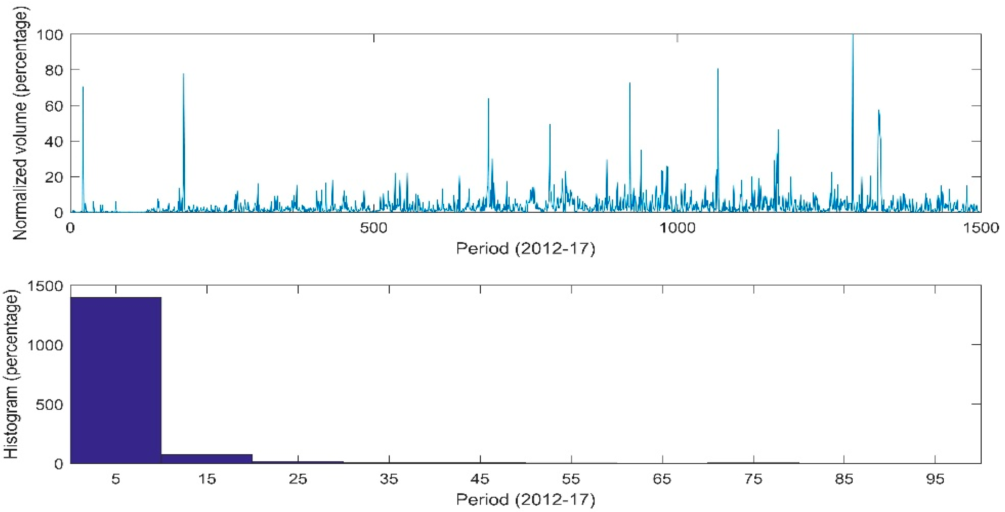
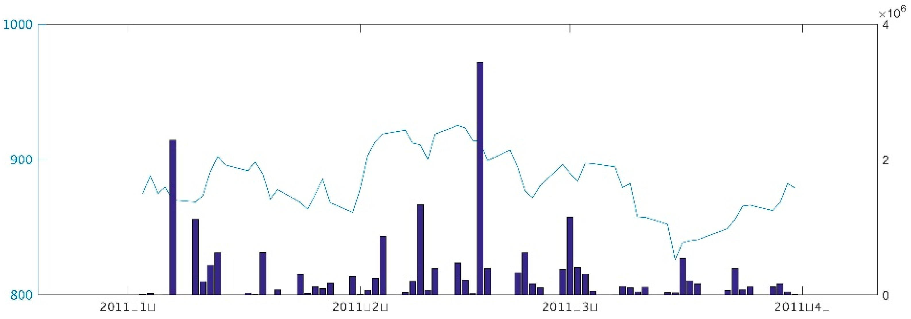
Stale prices are likely to produce artificially good forecasts as the estimate for the volatility of the stock is likely underestimating the real volatility. In Figure 1 the normalized traded volume for the 2012 to 2017 period can be seen. The normalization was done by dividing the daily traded volume in the market by the maximum traded volume in a single day during that period. During 120 days, representing approximately 8.0% of the days, the traded volume did not reach 0.05% of the total peak traded volume. In 401 days, accounting for 26.8% of the total days, the traded volume did not reach 0.5%. In Figure 2 shows an extreme example for illustrative purposes. For the three months period from 5 January 2011 to 31 March 2011 there were four days in which there appears an ending price level for the index but there is no recorded traded volume. It should be noted that this period was not included in the analysis and that it is shown only as an example. For the majority of the other indexes the issues of stale prices and data availability were not as apparent as in the case of Namibia.
2. Methods
We analyzed equity indexes from ten countries which are typically associated with narrow or deep markets. These ten countries were grouped into four categories according to the perceived narrowness of its equity capital market. Those four categories were: (1) very deep, (2) deep, (3) moderately narrow and (4) narrow. The US equity market is so large and deep that it is really on a category of its own and was the only country selected for the very deep category. The Dow Jones index was selected as a representative index for the US equity market. The deep category is composed of the FTSE (UK), DAX (Germany) and CAC (France) indexes. The moderately narrow category contains the CSI (China), IBEX (Spain) and RIGSE (Latvia) indexes. The Chinese equity market is one of the largest in the world, but it is typically associated with narrow markets because of the high proportion of retail (individual) investors compared to other markets in which institutional investors account for the bulk of the trading volume. The Chinese equity market is a liquid market, but it is likely not very efficient from a pricing point of view due to this large proportion of individual investors. The market indexes for Tunisia, Tanzania and Namibia were included in the narrow category. A list of all the indexes is showed in Table 1.
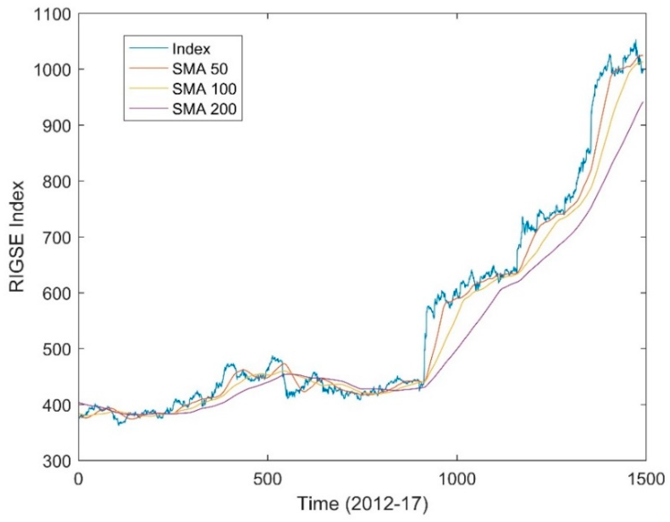
Daily closing prices of the indexes for the period from 2012 to 2017 were obtained from Bloomberg. The 50, 100 and 200 day moving averages were also calculated for each of the previously mentioned indexes. The moving average at any given time is just the average price over a predetermined number of previous days, see Equation (1). For instance, the 50 day moving average will be the sum of the closing prices over the last 50 days divided by 50. In Figure 3 an example for the RIGSE index and its 50-day, 100-day and 200-day moving averages can be seen.
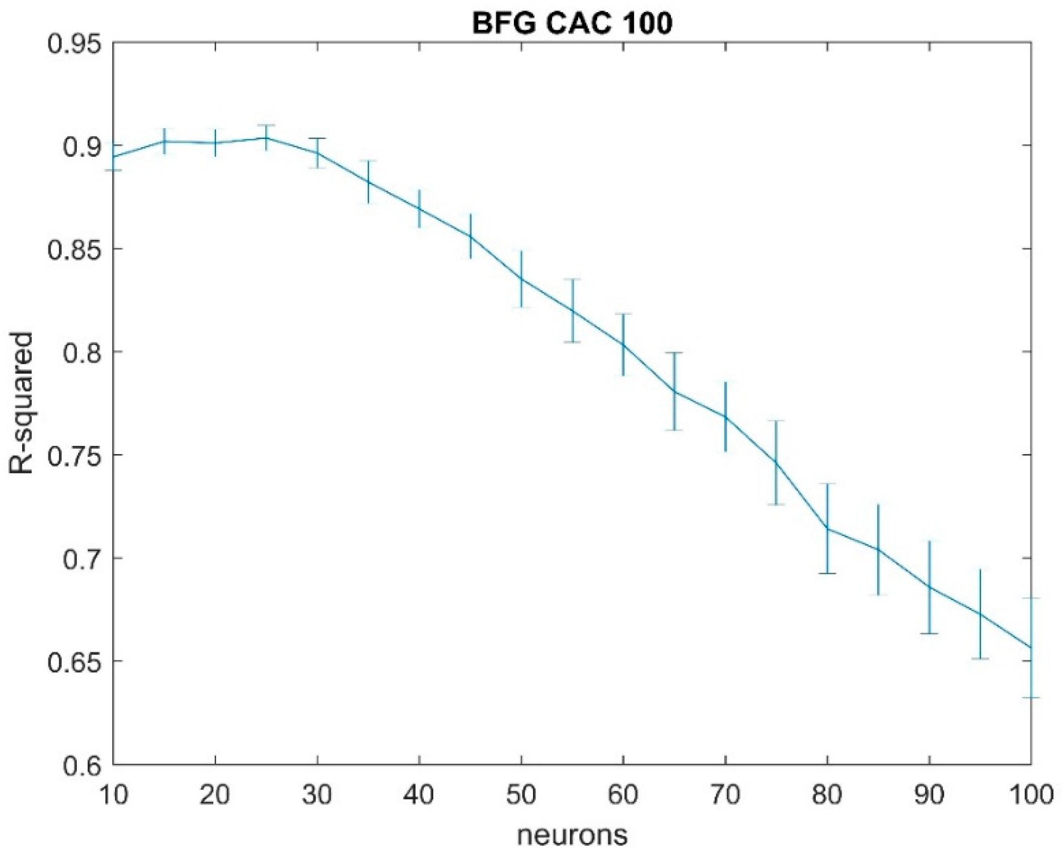
The forecasting capability of neural networks for all the previously mentioned ten indexes, representing very deep, deep, moderately narrow and narrow markets were estimated. The structure followed for the neural network consisted of one hidden layer. The amount of neurons was increased from 10 to 100 in steps of 5. Then, the network was created using an input of one of the moving averages and the index as the target value. The process was repeated for all three moving averages (50-day, 100-day and 200-day). Due to different randomly generated initial conditions two neural networks with the same inputs, output and structure are likely to generate slightly different results (forecasts). In order to account for that 100 networks were estimated for each configuration. Each of these forecasts was regressed against the actual target. In this way a probability distribution for the R-square value was obtained. The standard procedure of setting aside 15% of the data for testing purposes was followed. It will be shown that increasing the number of neurons, for most cases, did not increase the accuracy of the forecasts. The opposite was actually true in many cases with accuracy gradually declining. A typical outcome can be seen in Figure 4.
2.1. Training Algorithms
In this section a very brief description of the training algorithms used for the neural networks is shown. All of them are well-known algorithms with applications in several areas. All the actual implementation of the algorithms was done in Matlab [30] and we followed, for clarity purposes, its notation and acronyms.
2.1.1. Quasi Newton
The quasi Newton (BFG) [31] is a powerful and relatively fast training algorithm but it is costly from a computing power requirement point of view. The basic algorithm is showed in Equation (2).
2.1.2. Conjugate Gradient
Conjugate gradient methods, described in Equations (3) and (4), are a popular training algorithm tool. In its most common version, it is done through an iterative process in which the steepest direction is followed, following in the first iterative step the negative value of the gradient. In the next iteration it follows the previous value, multiplied by a distance factor and by a direction function:
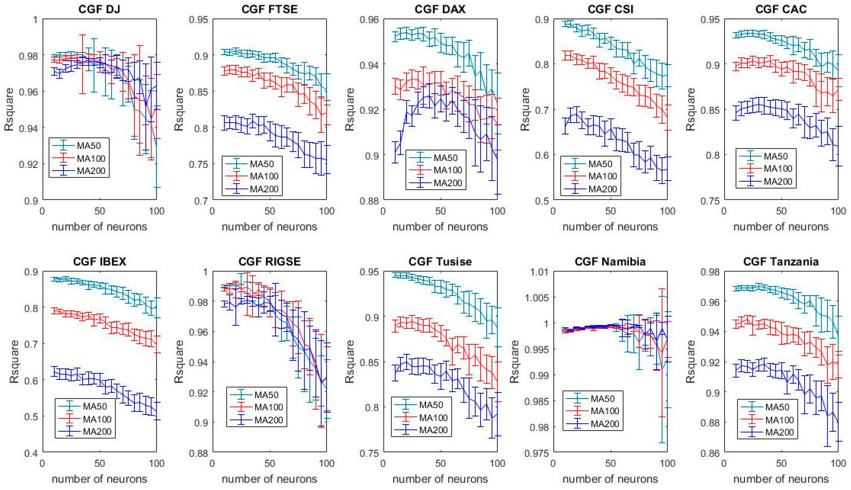
In the case of the Fletcher Reeves (CGF) algorithm [32] the parameter is calculated as described in Equation (5).
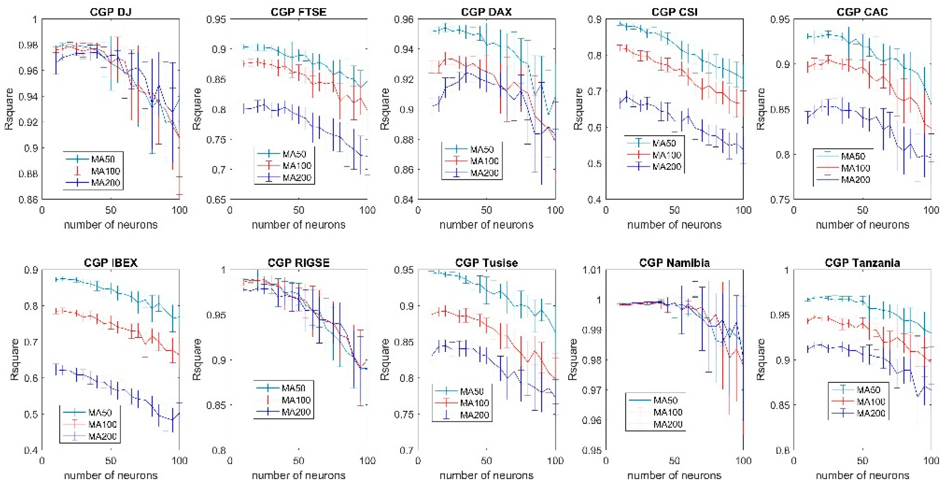
Another of the conjugate gradient variants is the Fletcher Powell (CGB) algorithm [35]. Powell describes the idea as automatically resetting the search direction (restart) and it is done according to some conditions on the orthogonality of the gradient at successive steps. If Equation (7) is satisfied, then the search direction is the negative value of the gradient.
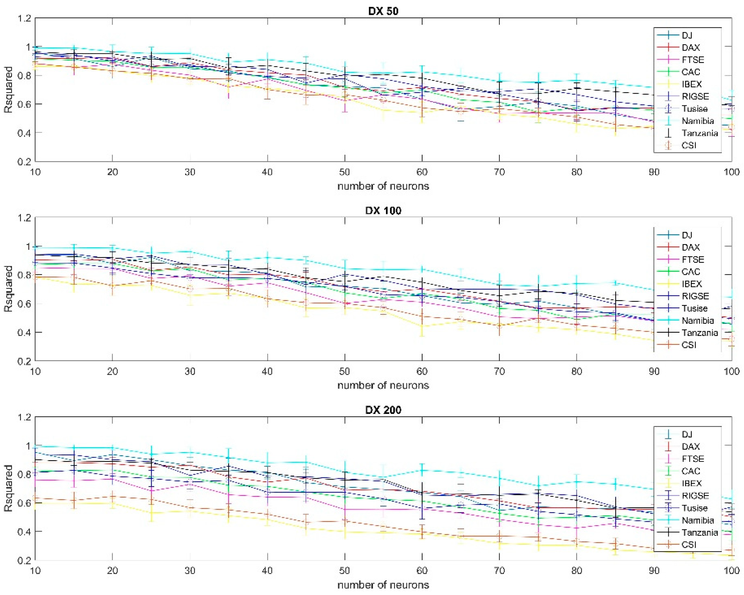
2.1.3. Gradient Descent
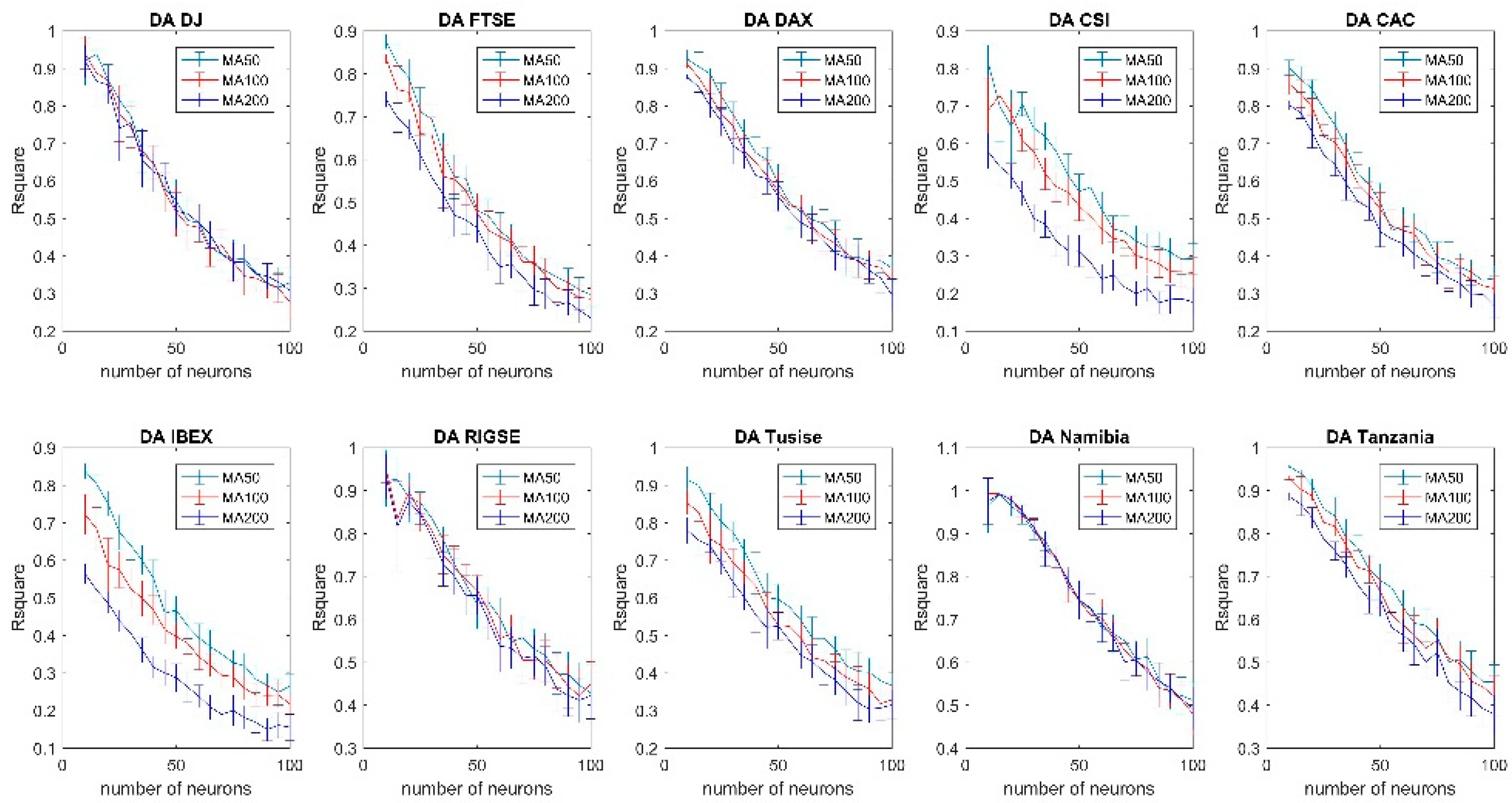
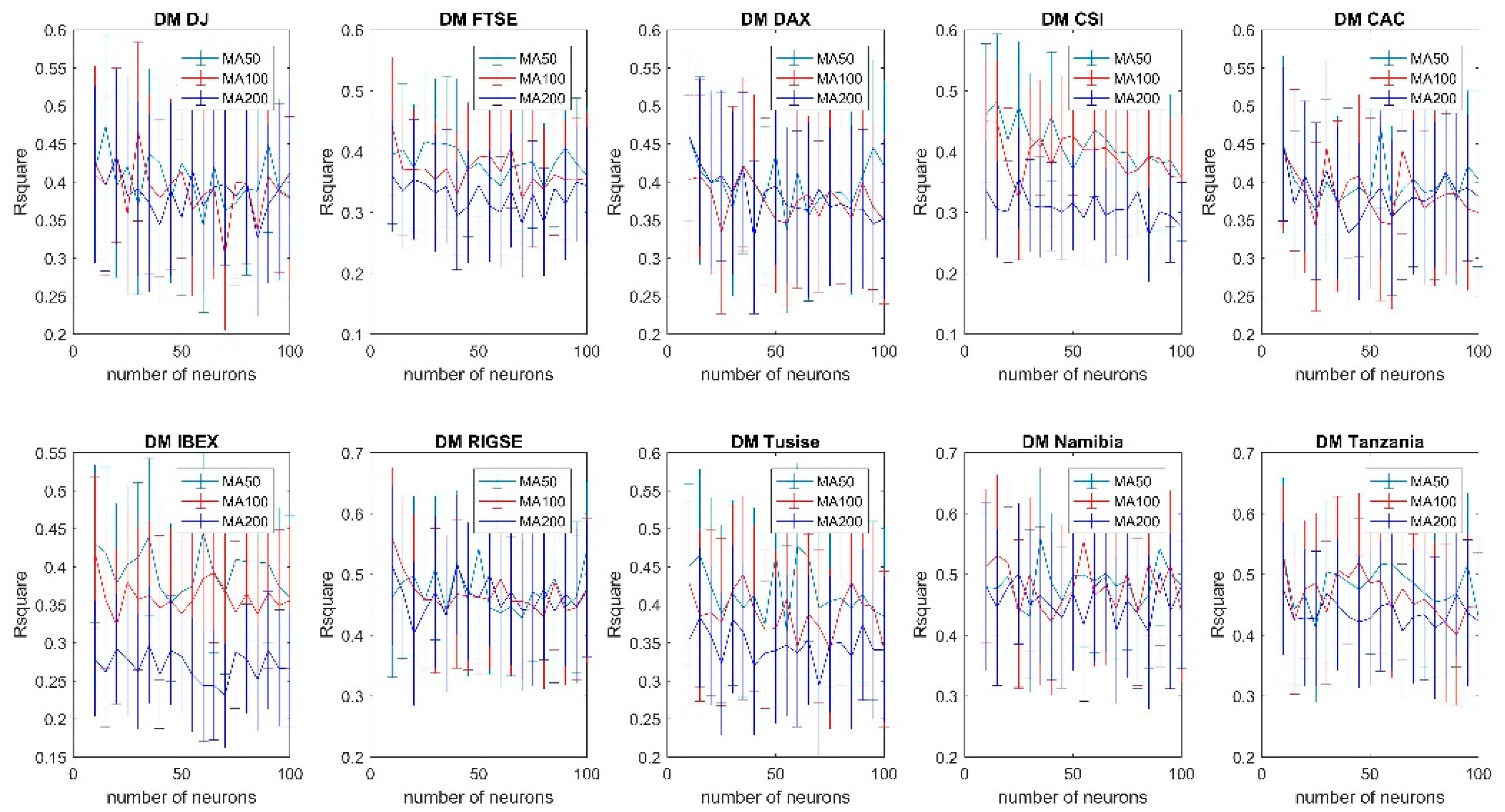
Gradient decent algorithms are among the most popular training techniques for neural networks due to their relative simplicity, and they use as the main component for the changes in each iteration the gradient. We use three different types of gradient descent algorithms. The first one was the gradient descent with momentum (DM) [30]. This algorithm adds momentum considerations in an attempt to avoid the issue of local minima. Another training algorithm used was the gradient descent with adaptive learning (DA) variant. In this approach the learning rate is dynamically adjusted, taking into consideration the accuracy of the forecasts in each iteration. A third variant used was a combination of the previous two. This method is called gradient descent with momentum and adaptive learning (DX).
2.1.4. Other Methods
We also used some other methods such as the Levenberg Marquardt (LM) approach. This is a relatively simple approach with moderate computational requirements. The basic iterative process is showed in Equation (8):
Another method used was the [36] Secant approach (OSS). This is a straightforward technique in which the iterative change in values is dictated by a function of the current gradient and the gradient in the previous iteration. The last technique used was resilient backpropagation (RP). This is another frequently used training algorithm in which the increase in each iteration is defined by Equation (9):
In total 10 learning algorithms were used, see Table 2, as a forecasting tool for the previously mentioned 10 country stock indexes. The moving average was used as an input for the neural network (the process was repeated for all the three moving averages considered). As previously mentioned, 15% of the data was designated as testing data and not used during the training period. The R-squared values showed in the results are the R-squared obtained when regressing the actual value with the estimated generated for the testing data set. This is the standard procedure to try to ensure that the trained neural network generalizes reasonably well when faced with new data, which is a critical step for neural networks. Choosing the appropriate learning algorithm for the neural network is of clear importance but it will be showed that there appear to be some general trends for all the ten learnings algorithms analyzed, supporting the hypothesis that neural networks are actually an appropriate forecasting tool for stock prices in narrow markets. Calculating 100 networks per index and per configuration allowed for the estimation of confidence intervals. This was done in order to avoid having results that are relatively accurate but that can be obtained because a one off or relatively unlikely events.
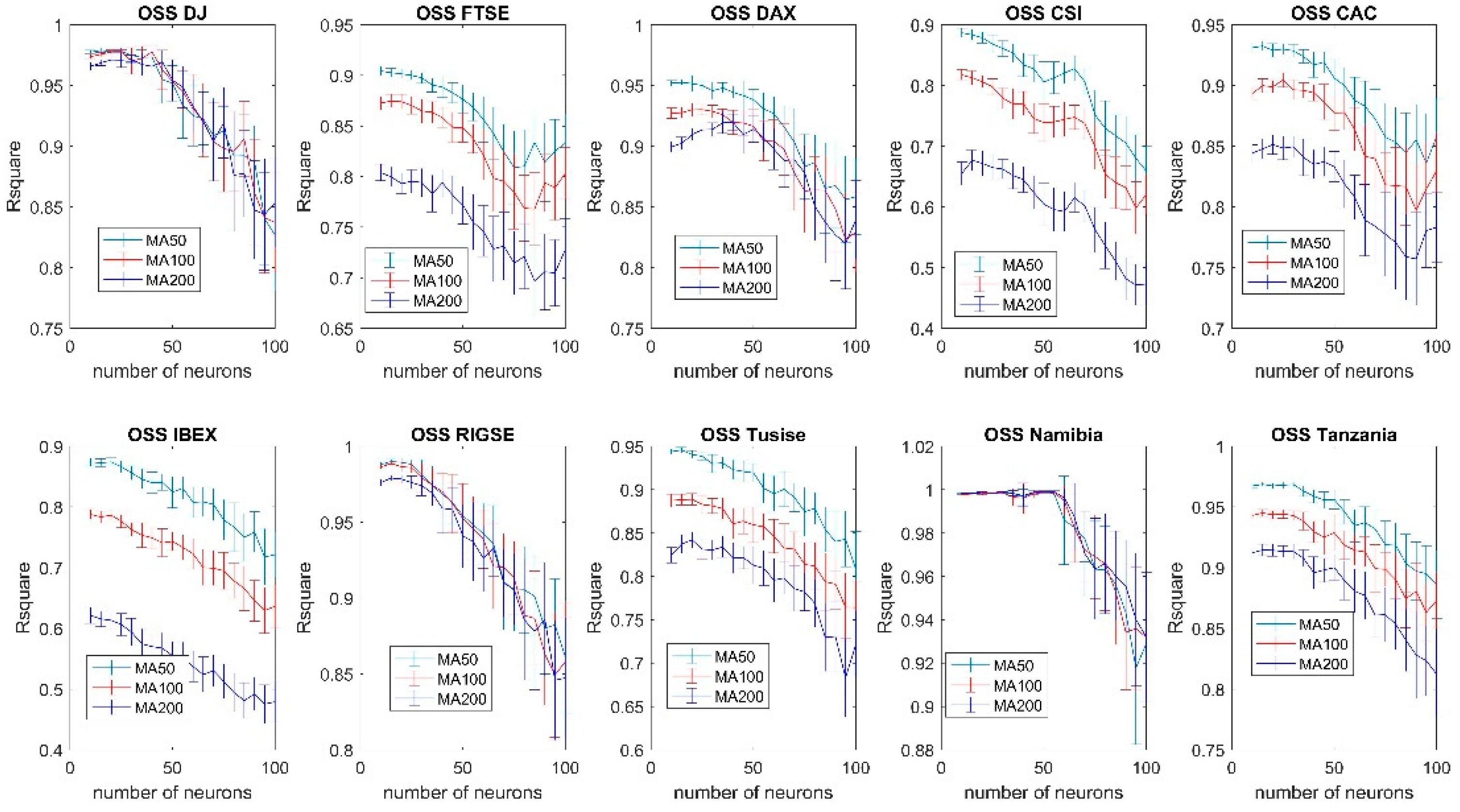
As an example, in Figure 5 it is shown the forecasting accuracy measured as the R-squared of the regression between the actual and forecasted values, using the OSS training algorithm, for all the indexes increasing the number of neurons and using the 50-day, 100-day and 200-day moving averages, which are denoted in the figures as MA50, MA100 and MA200. This analysis was carried out for all the previously mentioned 10 training algorithms. The results for all the other training algorithms can be seen in Appendix A (Figure A1, Figure A2, Figure A3, Figure A4, Figure A5, Figure A6, Figure A7, Figure A8 and Figure A9).
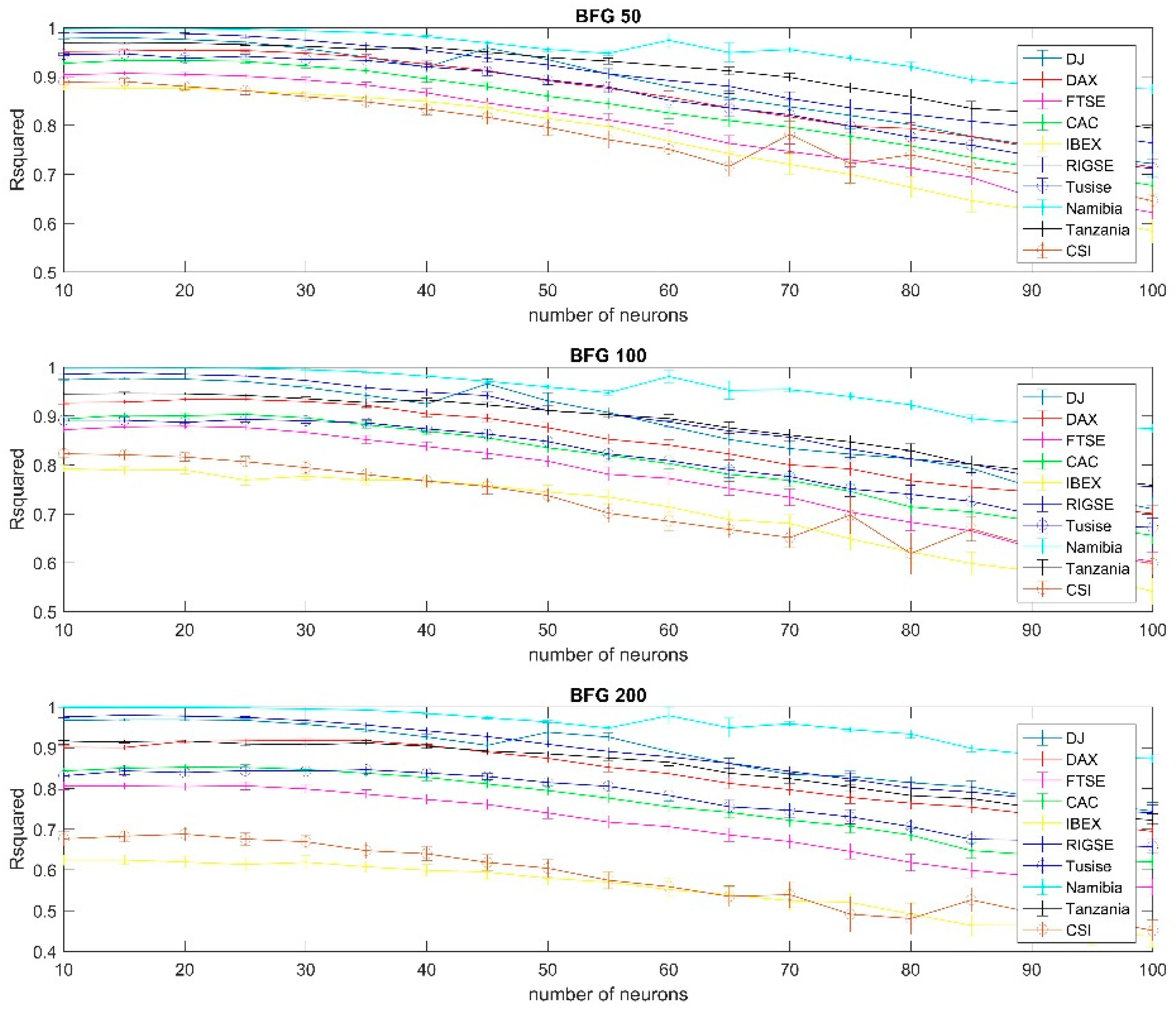
It could be also useful to compare how, given a specific configuration and choice of moving average, would the multiple neural network perform for each country, rather than just comparing several networks and moving averages for the same country index. In Figure 6 an example of this approach can be seen. This figure showed the accuracy of forecasts using the BFG training algorithm for all the indexes analyzed. The results for all other training algorithms can be seen in Appendix B (Figure A10, Figure A11, Figure A12, Figure A13, Figure A14, Figure A15, Figure A16, Figure A17 and Figure A18). The Namibian case appears to be the one with the best forecasting accuracy regardless of the choice of moving average but this is, as previously mentioned, likely a result of stale price as there were periods with no or very little market activity.
3. Results
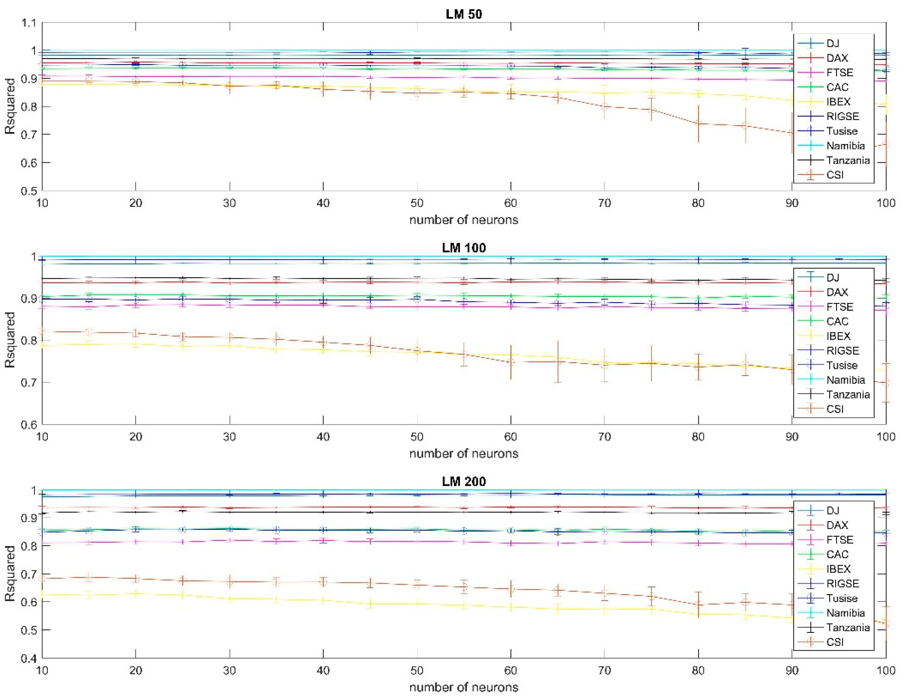
Of the models analyzed the best results, from a forecasting accuracy point of view, were those using the 50-day moving average and a relatively small number of neurons, typically 10. Increasing the number of neurons in the network did not increase the forecasting accuracy. This result was relatively consistent among most of the indexes, regardless if they belong to very deep, deep, moderately narrow or narrow categories, as well as across most of the training algorithms analyzed. The results in the Namibian case, a particularly narrow market, should be taken with caution and present some unique characteristics. The forecasts for the Namibian case appear to be remarkably accurate, see for instance Figure A8, but this could be related to the stale price issue and the accuracy hence overstated. Liquidity is very low in the Namibian case and occasionally the quoted price does not correspond with an executed trade that day but with the closing price on a previous day. The result in this way could appear to be very accurate but a practical application of such a model for trading purposes could lead to disappointing results if the price quoted does not match the price at which a transaction can be actually done. It is also interesting to notice (Figure A8) that in the case of Namibia, using the Levenberg Marquardt method the forecasting accuracy appears to increase as the number of neurons increases, which is not the case for the vast majority of other indexes and configurations. In this case there also appears to be no statistically significant difference between using the 50-day, 100-day or 200-day moving averages, which is again in direct contrast with the results from most of the other indexes. The case of Tanzania and Spain (IBEX) with the same configuration (Figure A8) are examples of typical results with the 50-day moving average generating better results than any of the other indexes analyzed and forecasting accuracy gradually decreasing as the number of neurons increases. It should also be noted that the forecasting accuracy of the Dow Jones index, using the same configuration, did marginally increase when the number of neurons were increased. Another peculiarity showed by the Dow Jones index is that the selection of the moving average (50-day, 100-day or 200-day) did not have a significant impact on the forecasting accuracy for most of the configurations analyzed.
3.1. Training Algorithm
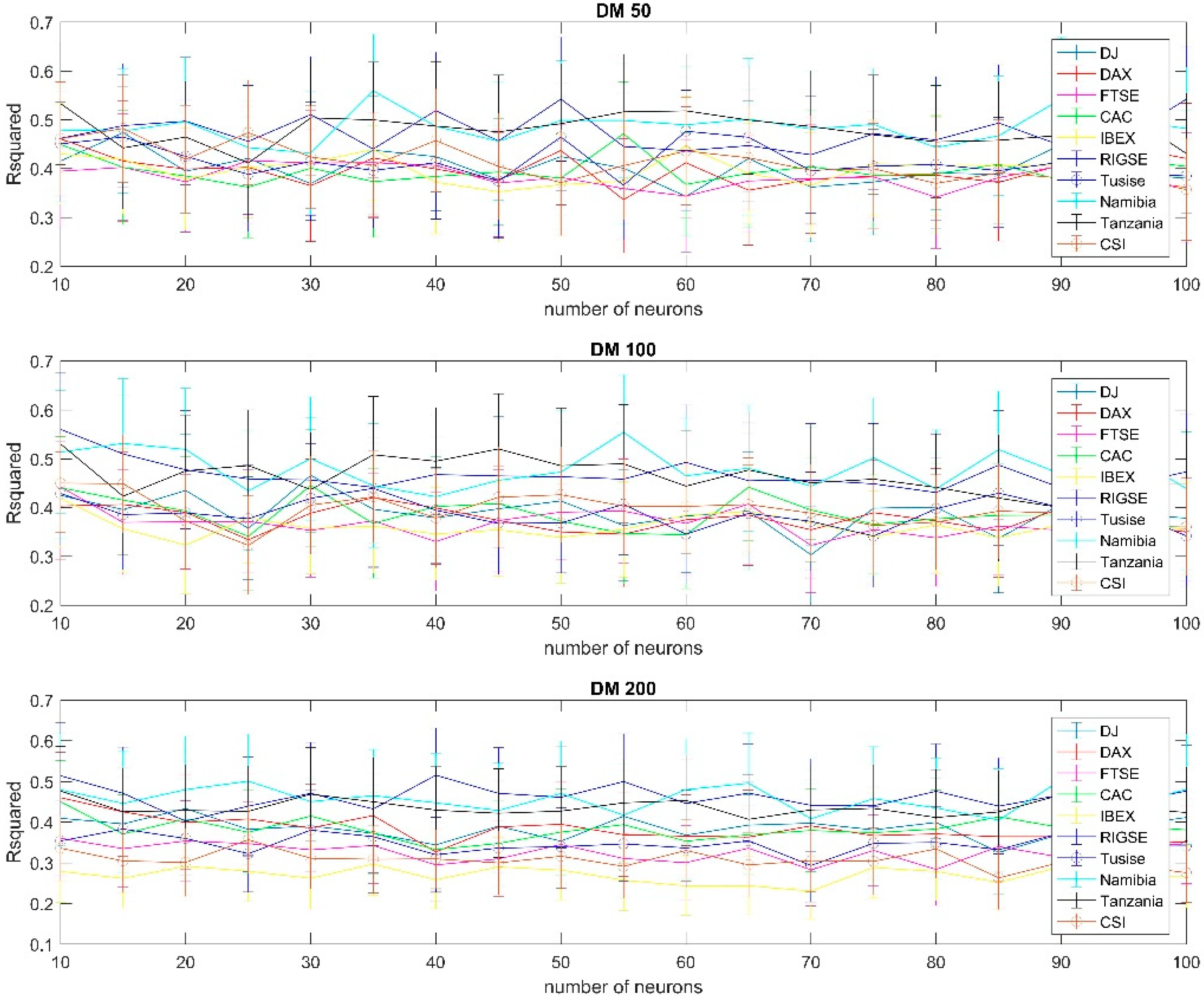
In general terms the accuracy of the training algorithms was comparable. One of the noticeable exceptions was the gradient descent momentum (Figure A6) that generated the worst results among all the training algorithms used. These poor results were obtained for all the 10 indexes and regardless of the number of neurons used. All the other training algorithms provided comparable results for the indexes regardless on the classification of the index. All the narrow and moderately narrow markets analyzed, with the previously mentioned caveat for the Namibian market, generated forecasts that are comparable to deep and very deep markets.
3.2. Indexes
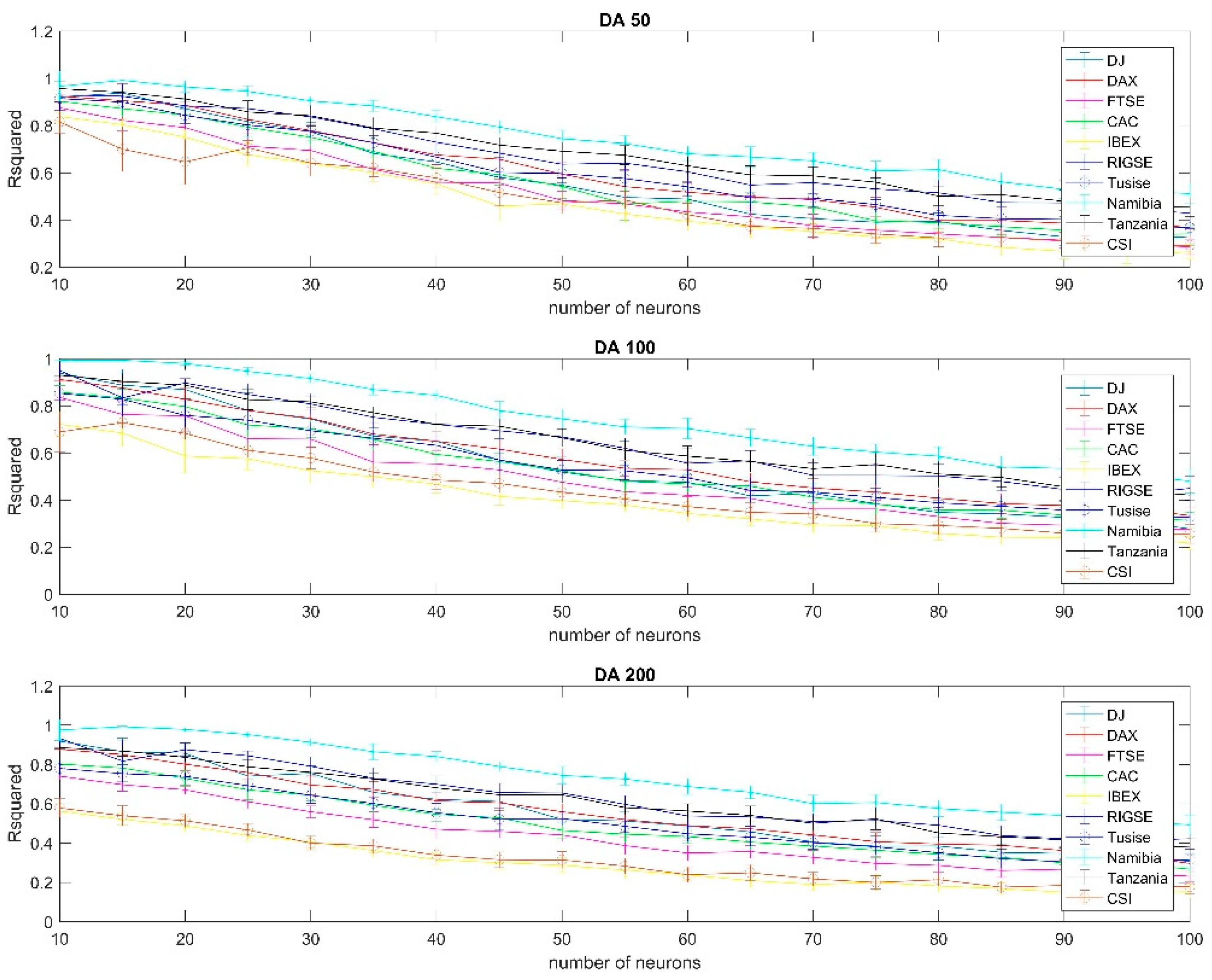
While the forecasting accuracy is good for all the indexes, regardless if it is a narrow market or not, there are some apparent differences with for instance moderately narrow markets, particularly in the case of the Spanish (IBEX) and Chinese (CSI) generating for most of the configurations analyzed slightly poorer forecasts than in the case of the other indexes, see for instance Figure 6 and Figure A11. The difference appears to be particularly large in the case of the gradient descent with adaptive learning (Figure A12).
4. Discussion
Neural networks appear to be an applicable tool for stock forecasting purposes on narrow markets with performance that is comparable but typically lower than in deeper markets. Forecasts in some particularly narrow markets might appear to be very accurate but that could be related to stale prices. This phenomenon appear when the quoted price is not representative of an actual transaction on the analyzed day but of some transaction on a previous day. This is typically associated with illiquid markets. Besides, for this type of extreme case, it would appear that neural networks do a relatively good job forecasting stock performance in the countries analyzed. The 50-day moving average provided results that were at least statistically not worse than the 100-day or 200-day moving averages for most of the neural network configurations analyzed. For other, deeper, markets, such as the U.S. market, there appears to be less statistically significant differences between these different moving averages regarding forecasting accuracy. It should also be noted that increasing the number of neurons did, in most cases, not only not increase forecasting accuracy but it decreased it. This was a general trend observed when using virtually all of the training algorithms with basically all the ten stock indexes analyzed. This might be related to the issue of local minima in neural networks. As the number of neurons increases the neural network might get stuck in a local minimum, basically losing generalization power. Therefore, an important takeaway is that naively increasing the level of complexity of a neural networks, by adding large amounts of neurons to the network, is not likely to translate into more accurate stock forecasts.
The fact that neural networks appear to be applicable for stock forecasting in narrow markets suggest that while there are clearly very big differences between narrow and deep markets they might also share some features that allow the successful use of the same forecasting technique, such as neural networks, in both types of markets. As previously mentioned the flow of information is likely very different in some of the narrow markets analyzed, with relatively poor telecommunication and trading infrastructure, compared to countries such as the United States, but, interestingly, it appears that regardless of these obvious differences neural networks have comparable levels of applicability, for stock forecasting purposes, in narrow and deep markets.
5. Conclusions
Besides the many differences between narrow and deep stock markets it appears that neural networks are an efficient forecasting tool for both types of markets. This is a rather surprising result as the differences between those markets could be rather large with the basic expectation being that their behavior and, hence, the appropriate tool for forecasting the dynamics of its stock markets being rather different. This does not appear to be the case with neural networks generating relatively accurate forecasts for narrow, moderately narrow, deep and very deep markets. Just to put it into perspective, the results suggest that the same technique (neural network) of stock forecasting is applicable to stock markets as different as the ones in Namibia, Tanzania and the United States. One issue that should however be taken into account is that some of those are narrow stock markets, particularly in the case of Namibia is stale prices. Some of the prices quoted in a narrow stock market might not reflect the “true” price of a stock as for example that stock might not have traded in a given day with the price quoted being that of the previous day. That would decrease the volatility of the quoted stock prices, compared to the actual price of the stocks (at which a stock transaction can be actually carried out). This reduction in volatility might make the forecasting task easier but less reliable as an investment tool. Nevertheless, even after accounting for the issue of stale prices it would appear that neural networks can be successfully applied to different stocks markets with varying degrees of narrowness.
It is interesting that the results, while comparable, seem to indicate that the forecast for moderately narrow markets are slightly less accurate than those for deep markets. This might be due to the previously mentioned differences in quality and reliability of the information and trading platform in those markets. It is also interesting to observe that the results support the idea that the analyzed markets are not perfectly efficient, even those that are very deep, as forecasting tools such as neural network are able, using only historical data (moving averages are constructed using only historical data) to generate relatively accurate forecasts, which would seem to contradict the efficient market hypothesis, which is a result in line with other paper analyzing the predicting capabilities of neural networks in the stock market. Perhaps one of the most important takeaways is that the results support the hypothesis that both narrow and deep markets are not perfectly efficient and that stock forecasting tools can be used successfully.
Author Contributions
Conceptualization, G.A. and D.R.R.; methodology, G.A.; software, G.A. and D.R.R.; validation, G.A. and D.R.R.; formal analysis, G.A. and D.R.R.; investigation, G.A. and D.R.R.; resources, G.A. and D.R.R.; data curation, G.A.; writing—original draft preparation, G.A.; writing—review and editing, G.A. and D.R.R.; visualization, G.A. and D.R.R.; supervision, G.A. and D.R.R.; project administration, G.A. and D.R.R.; funding acquisition, D.R.R. All authors have read and agreed to the published version of the manuscript.
Funding
This work has received support by Ministerio de Ciencia e Innovación of Spain under project PID2019-106212RB-C41.
Conflicts of Interest
The authors declare no conflict of interest.
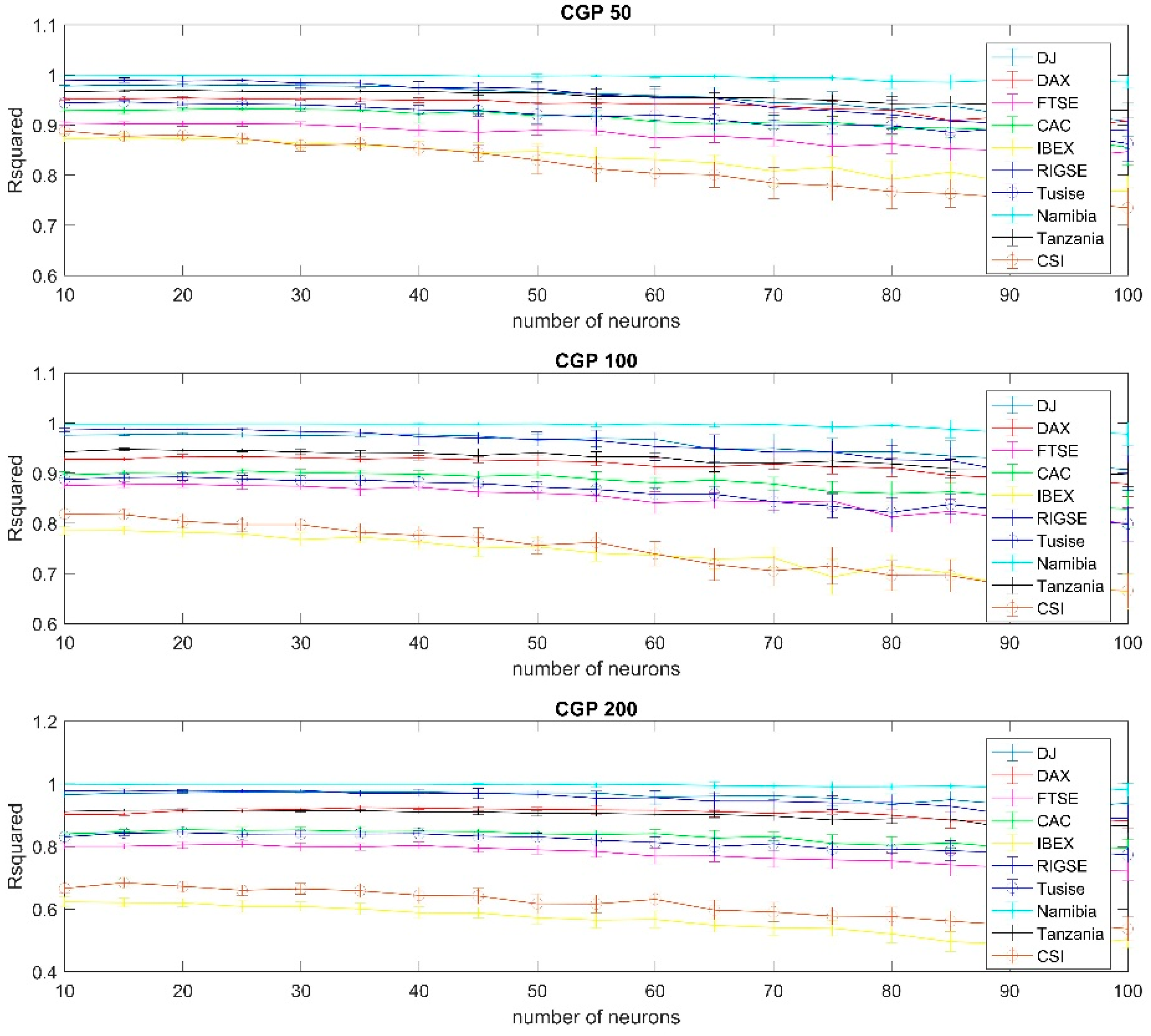
Appendix A
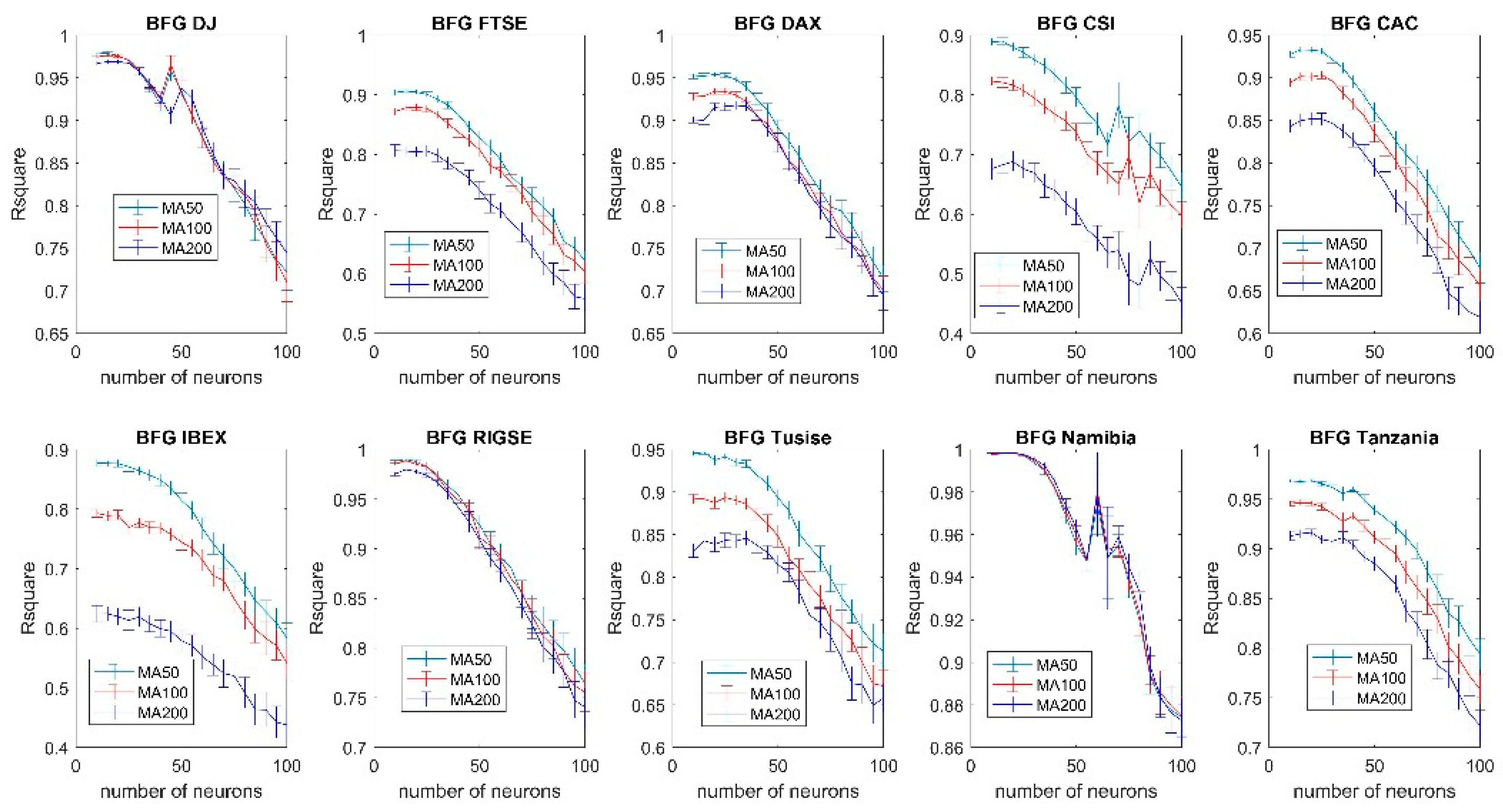
Each graph in this appendix contains the evolution of the forecasting accuracy as the number of neurons is increased, for all the different stock indexes analyzed for a given learning algorithm, for instance, Figure A1 shows how the forecasting accuracy, measured as R-squared, tends to decrease as the number of neurons increases for all the equity index (see Table 1) for the quasi Newton learning algorithm (BFG). In Table 2 it can be seen the key for the abbreviations of the different learning algorithms.
Figure A1.
Forecasting accuracy comparison of different moving averages using the quasi Newton (BFG) training algorithm (99% confidence interval).
Figure A1.
Forecasting accuracy comparison of different moving averages using the quasi Newton (BFG) training algorithm (99% confidence interval).

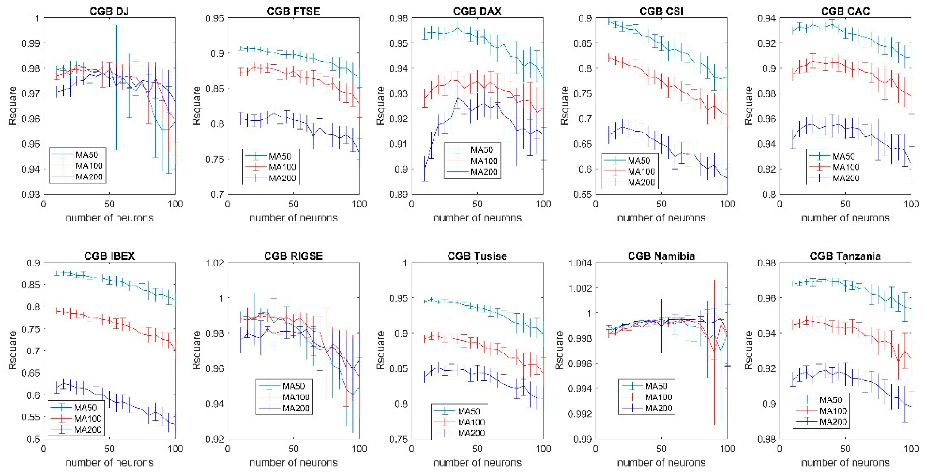
Figure A2.
Forecasting accuracy comparison of different moving averages using the conjugate gradient (with restarts) training algorithm (99% confidence interval).
Figure A2.
Forecasting accuracy comparison of different moving averages using the conjugate gradient (with restarts) training algorithm (99% confidence interval).

Figure A3.
Forecasting accuracy comparison of different moving averages using the conjugate gradient Fetcher Powell training algorithm (99% confidence interval).
Figure A3.
Forecasting accuracy comparison of different moving averages using the conjugate gradient Fetcher Powell training algorithm (99% confidence interval).

Figure A4.
Forecasting accuracy comparison of different moving averages using the conjugate gradient Polak Ribiere training algorithm (99% confidence interval).
Figure A4.
Forecasting accuracy comparison of different moving averages using the conjugate gradient Polak Ribiere training algorithm (99% confidence interval).

Figure A5.
Forecasting accuracy comparison of different moving averages using the gradient descent (adaptive learning) training algorithm (99% confidence interval).
Figure A5.
Forecasting accuracy comparison of different moving averages using the gradient descent (adaptive learning) training algorithm (99% confidence interval).

Figure A6.
Forecasting accuracy comparison of different moving averages using the gradient descent (momentum) training algorithm (99% confidence interval).
Figure A6.
Forecasting accuracy comparison of different moving averages using the gradient descent (momentum) training algorithm (99% confidence interval).

Figure A7.
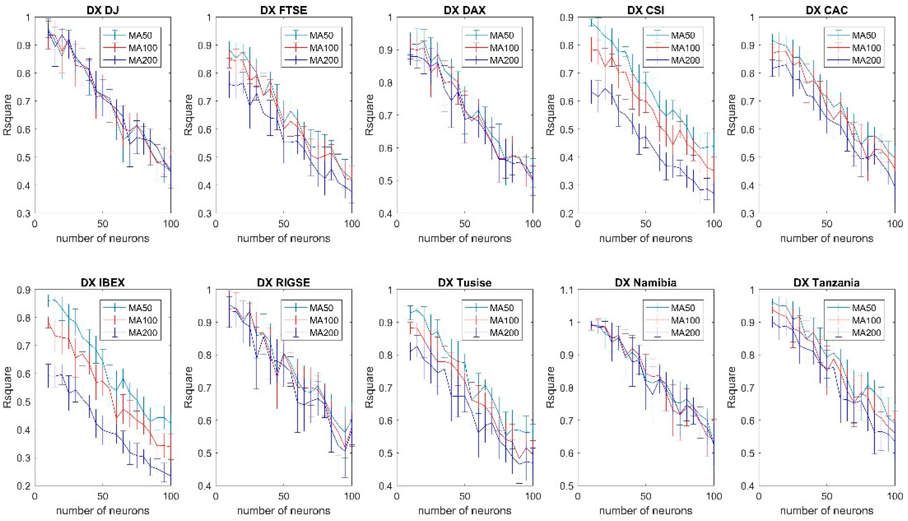
Forecasting accuracy comparison of different moving averages using the gradient descent (momentum and adaptive learning) training algorithm (99% confidence interval).
Figure A7.
Forecasting accuracy comparison of different moving averages using the gradient descent (momentum and adaptive learning) training algorithm (99% confidence interval).

Figure A8.
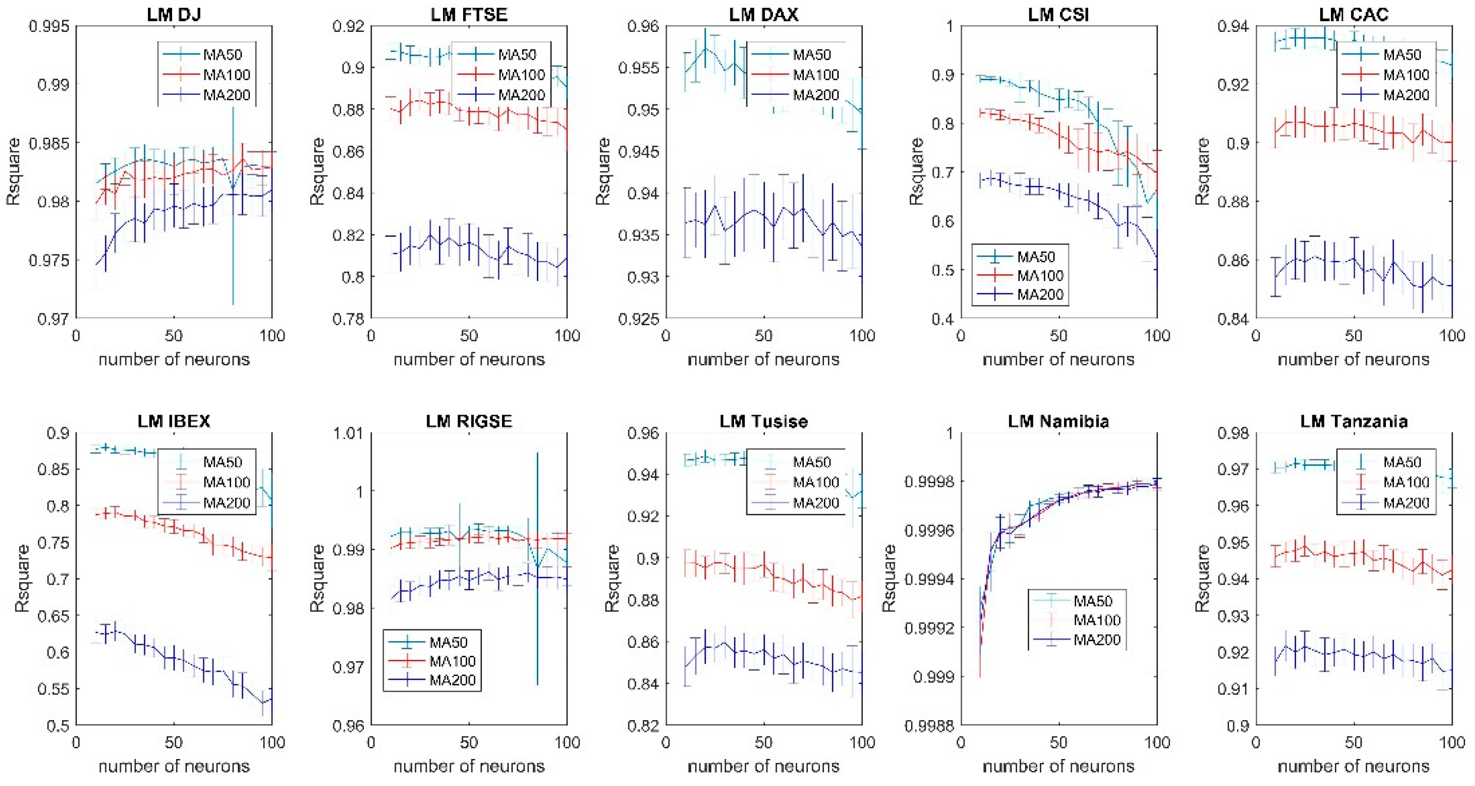
Forecasting accuracy comparison of different moving averages using the Levenberg Marquardt training algorithm (99% confidence interval).
Figure A8.
Forecasting accuracy comparison of different moving averages using the Levenberg Marquardt training algorithm (99% confidence interval).

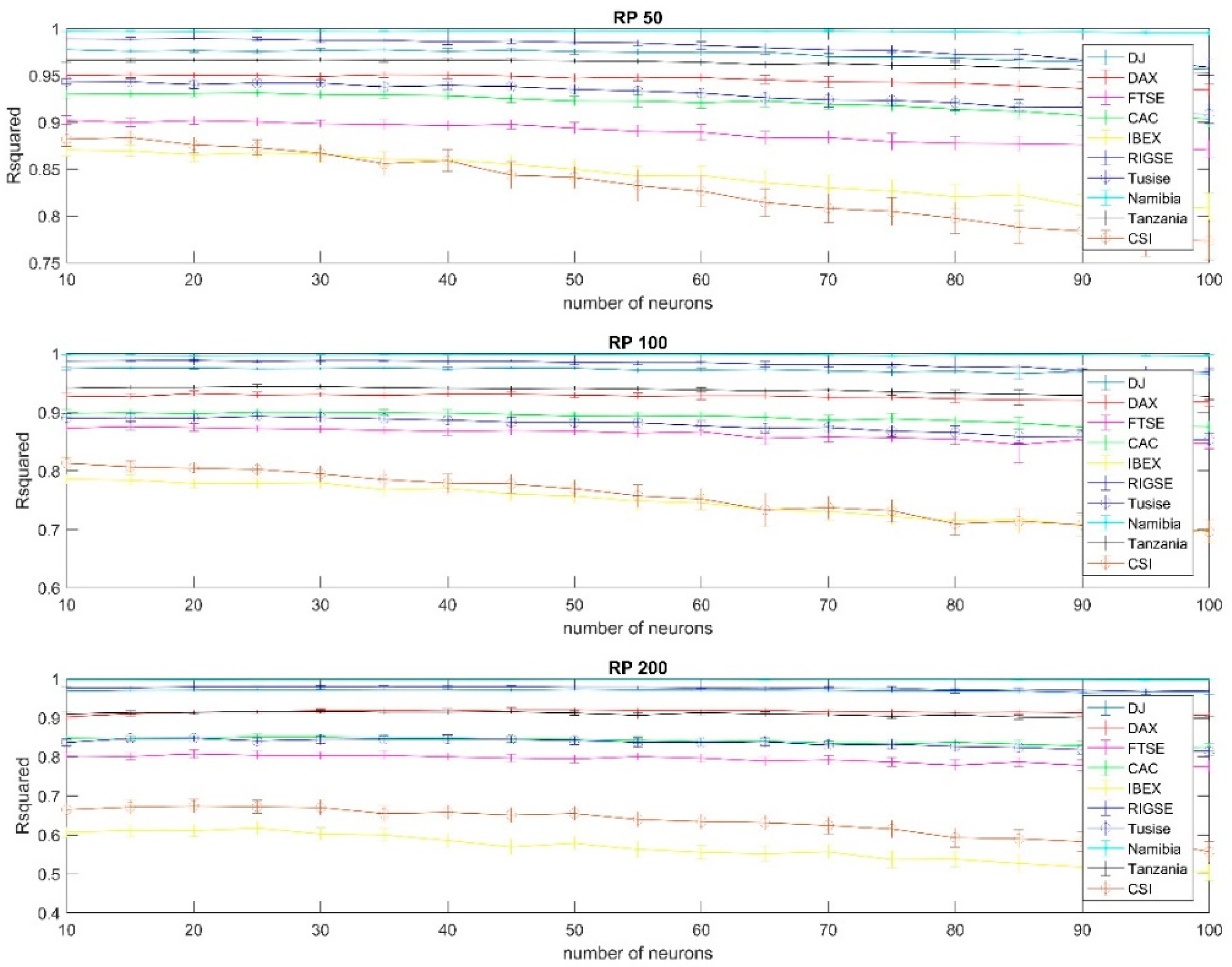
Figure A9.
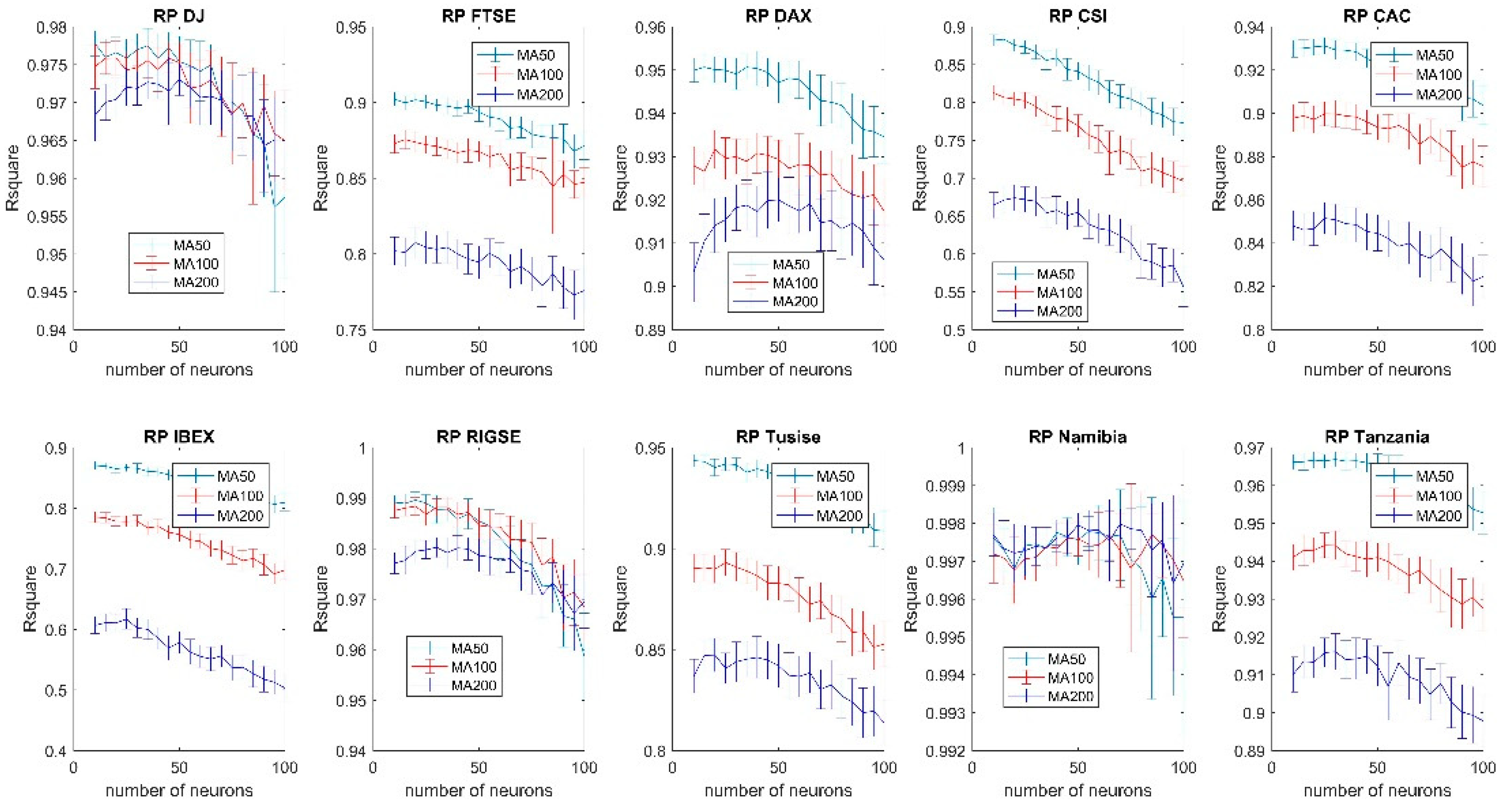
Forecasting accuracy comparison of different moving averages using the resilient backpropagation training algorithm (99% confidence interval).
Figure A9.
Forecasting accuracy comparison of different moving averages using the resilient backpropagation training algorithm (99% confidence interval).

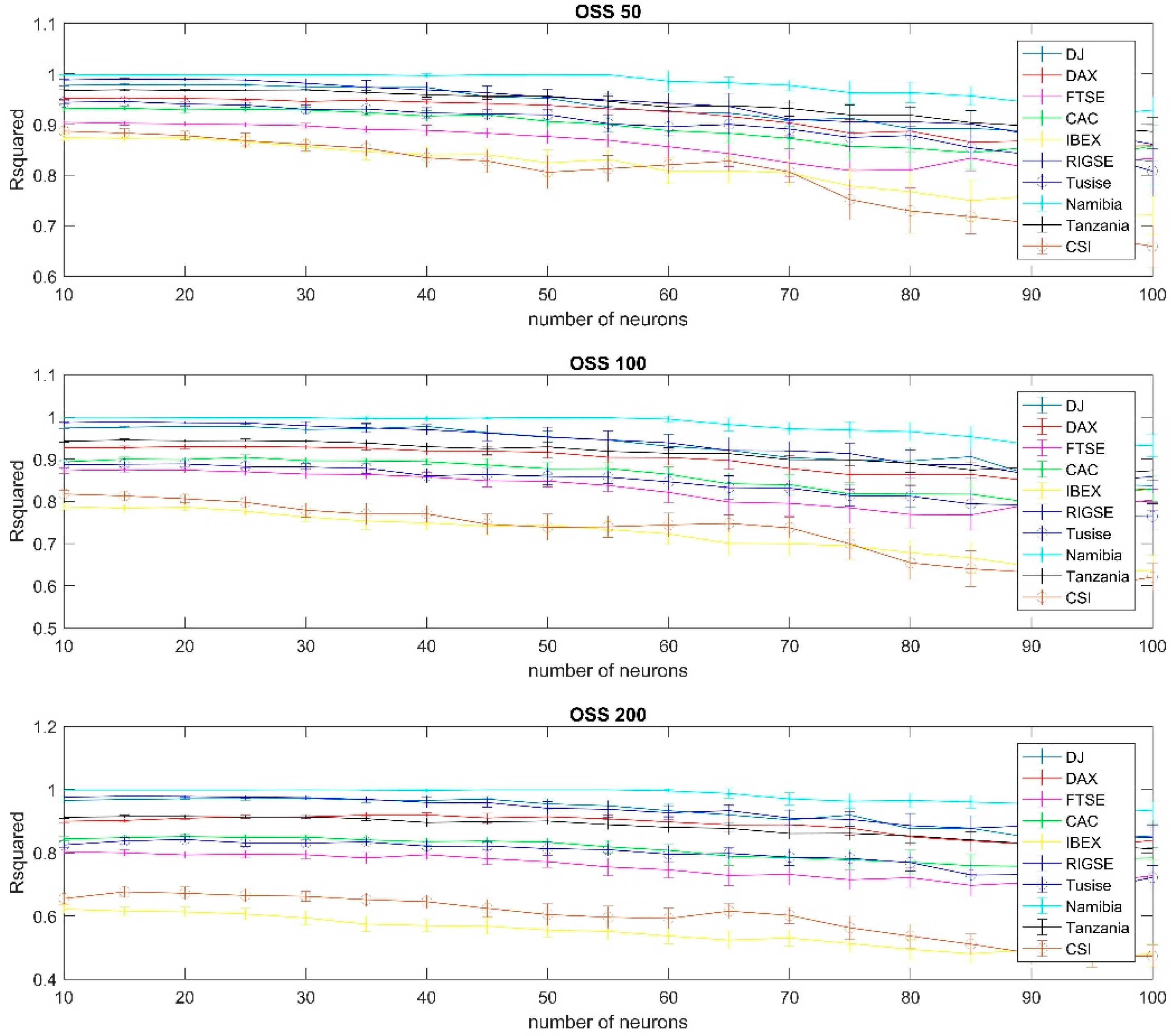
Appendix B
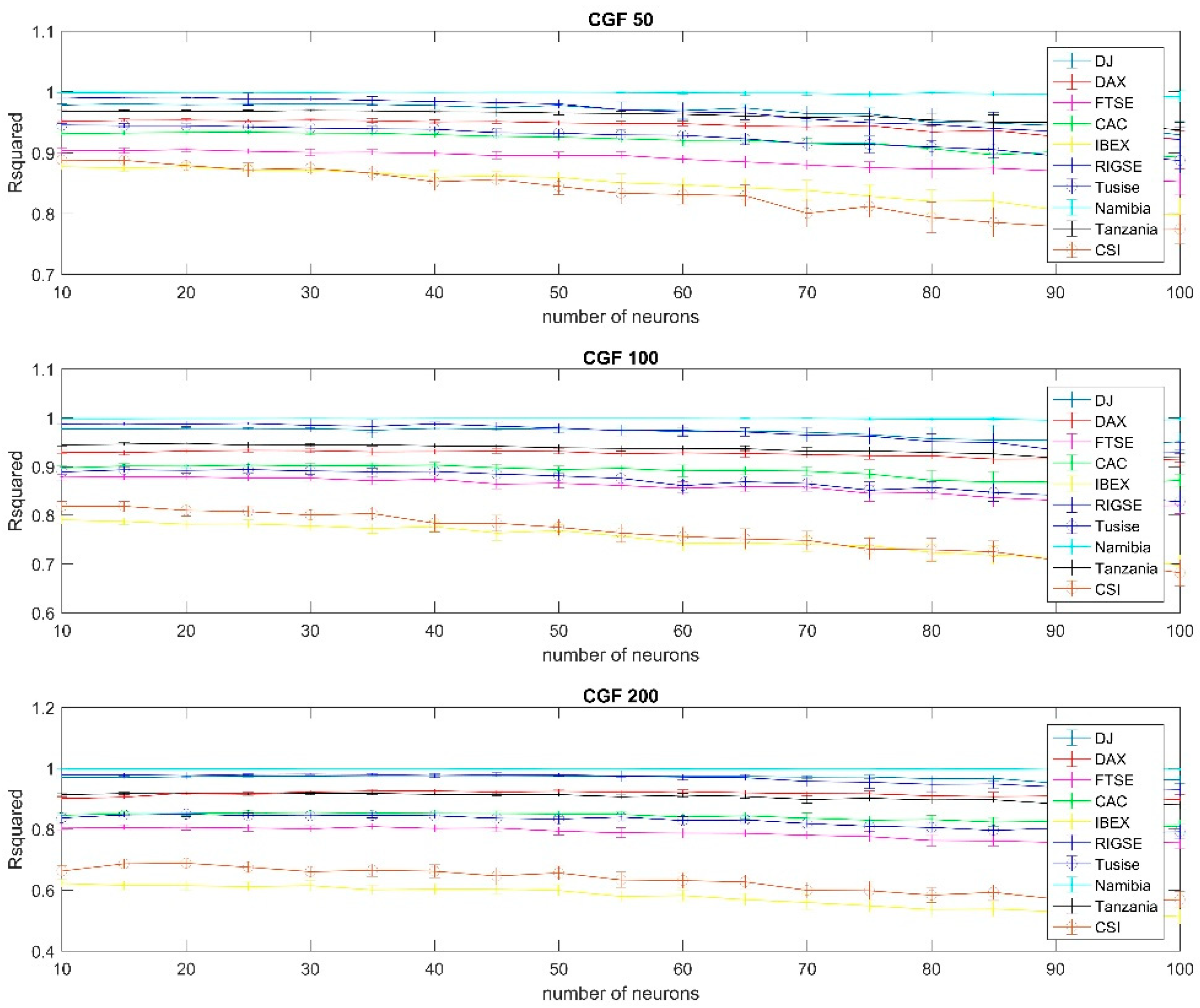
In this appendix every figure is divided into three subplots. From top to bottom this graph represents the analysis for the 50, 100 and 200 days moving averages showing how the forecasting accuracy evolves as the number of neurons is increased. For instance, Figure A10 illustrates the evolution of the forecasting accuracy of the conjugate gradient (with restarts) learning algorithm for all the ten stock indexes considered in this paper.
Figure A10.
Results using conjugate gradient (with restarts) training per country, 99% confidence interval, using the 50, 100 and 200 days moving average.
Figure A10.
Results using conjugate gradient (with restarts) training per country, 99% confidence interval, using the 50, 100 and 200 days moving average.

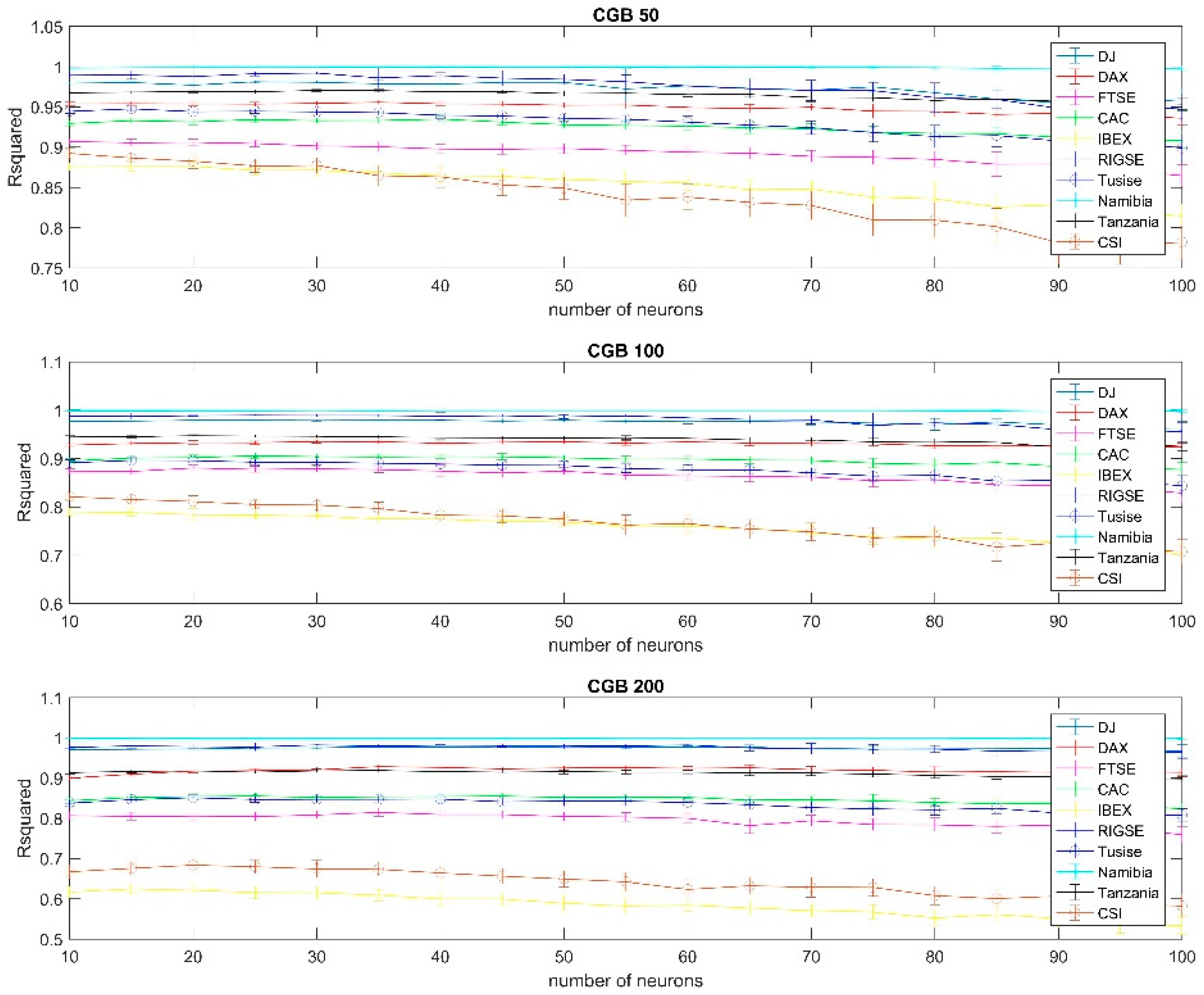
Figure A11.
Results using conjugate gradient Fetcher Powell training per country, 99% confidence interval, using the 50, 100 and 200 days moving average.
Figure A11.
Results using conjugate gradient Fetcher Powell training per country, 99% confidence interval, using the 50, 100 and 200 days moving average.

Figure A12.
Results using gradient descent (adaptive learning) training per country, 99% confidence interval, using the 50, 100 and 200 days moving average.
Figure A12.
Results using gradient descent (adaptive learning) training per country, 99% confidence interval, using the 50, 100 and 200 days moving average.

Figure A13.
Results using gradient descent (momentum) training per country, 99% confidence interval, using the 50, 100 and 200 days moving average.
Figure A13.
Results using gradient descent (momentum) training per country, 99% confidence interval, using the 50, 100 and 200 days moving average.

Figure A14.
Results using Levenberg Marquardt training per country, 99% confidence interval, using the 50, 100 and 200 days moving average.
Figure A14.
Results using Levenberg Marquardt training per country, 99% confidence interval, using the 50, 100 and 200 days moving average.

Figure A15.
Results using Secant training per country (99% confidence interval).

Figure A16.
Results using resilient backpropagation training per country, 99% confidence interval, using the 50, 100 and 200 days moving average.
Figure A16.
Results using resilient backpropagation training per country, 99% confidence interval, using the 50, 100 and 200 days moving average.

Figure A17.
Results using Polak Ribiere training per country, 99% confidence interval, using the 50, 100 and 200 days moving average.
Figure A17.
Results using Polak Ribiere training per country, 99% confidence interval, using the 50, 100 and 200 days moving average.

Figure A18.
Results using gradient descent with momentum and adaptive learning training per country, 99% confidence interval, using the 50, 100 and 200 days moving average.
Figure A18.
Results using gradient descent with momentum and adaptive learning training per country, 99% confidence interval, using the 50, 100 and 200 days moving average.

References
- Whang, J.; Wang, J.; Zhang, Z.; Guo, S. Forecasting stock indices with back propagation neural network. Expert Syst. Appl. 2011, 38, 14346–14355. [Google Scholar] [CrossRef]
- Zhang, G.; Patuwo, B.; Hu, N. Forecasting with artificial neural networks: The state of the art. Int. J. Forecast. 1998, 14, 35–62. [Google Scholar] [CrossRef]
- Zhang, L.; Suganthan, P. A Survey of randomized algorithms for training neural networks. Inf. Sci. 2016, 364, 146–155. [Google Scholar] [CrossRef]
- Cao, W.; Wang, X.; Ming, Z.; Gao, J. A review on neural networks with random weights. Neurocomputing 2018, 275, 278–287. [Google Scholar] [CrossRef]
- Zoicas-lenciu, A. The sensitivity of moving average trading rules performance with respect to methodological assumptions. Procedia Econ. Financ. 2015, 32, 1353–1361. [Google Scholar] [CrossRef] [Green Version]
- Johnston, F.; Boyland, J.; Meadows, M.; Shale, E. Some properties of a simple moving average when applied to forecasting a time series. J. Oper. Res. Soc. 1999, 50, 758–766. [Google Scholar] [CrossRef]
- Gencay, R.; Stengos, T. Moving average rules, volume and the predictability of security returns with feedforward networks. J. Forecast. 1999, 50, 758–766. [Google Scholar] [CrossRef]
- Larson, M. Moving Average Convergence/Divergence (MACD); Wiley: New York, NY, USA, 2007. [Google Scholar]
- Raudys, A.; Lenciasuskas, V.; Malcius, E. Moving averages for financial data smoothing. Information and Software Technologies. In Communications in Computer and Information Science, Proceedings of the ICIST 2013; Springer: Berlin/Heidelberg, Germany, 2013; Volume 403, pp. 34–45. [Google Scholar] [CrossRef]
- Granger, C. Forecasting stock market prices: Lessons for forecasters. Int. J. Forecast. 1992, 8, 3–13. [Google Scholar] [CrossRef]
- Shively, P. The nonlinear dynamics of stock prices. Q. Rev. Econ. Financ. 2003, 43, 505–517. [Google Scholar] [CrossRef]
- Wang, J.; Wang, J.; Zhang, Z.; Guo, S. Stock index forecasting based on a hybrid model. Omega 2012, 40, 758–766. [Google Scholar] [CrossRef]
- Barnes, P. Thin trading and stock market efficiency: The case of the Kuala Lumpur Stock Exchange. J. Bus. Financ. Account. 1986, 13, 609–623. [Google Scholar] [CrossRef]
- Bruand, M.; Gibson-Asner, R. The effects of newly listed derivatives in a thin stock market. Rev. Deriv. Res. 1998, 2, 58–86. [Google Scholar] [CrossRef]
- Ilkka, V.; Paavo, Y. Forecasting stock market prices in a thin security market. Omega 1987, 15, 145–155. [Google Scholar]
- Fama, E. Efficient Capital Markets: II. J. Financ. 1991, 46, 1575–1617. [Google Scholar] [CrossRef]
- Idowu, P.; Osakwe, C.; Kayode, A. Prediction of stock market in Nigeria using artificial neural network. Int. J. Intell. Syst. Technol. Appl. 2012, 4, 68–74. [Google Scholar] [CrossRef] [Green Version]
- Senol, D.; Ozturan, M. Stock price direction prediction using artificial neural network approach: The case of Turkey. J. Artif. Intell. 2008, 2, 70–77. [Google Scholar] [CrossRef] [Green Version]
- Samarawickrama, A.; Fernando, T. A recurrent neural network approach in predicting daily stock price an application to the Sri Lankan stock market. In Proceedings of the 2017 IEEE International Conference on Industrial and Information Systems (ICISS), Peradeniya, Sri Lanka, 15–16 December 2017. [Google Scholar]
- Apostolos, A.; Refenes, N. Stock performing modeling using neural networks: A comparative study with a regression model. Neural Netw. 1994, 7, 375–388. [Google Scholar] [CrossRef]
- Ballings, M.; Poel, D.; Hespeels, N.; Grip, R. Evaluating multiple classifiers for stock price direction prediction. Expert Syst. Appl. 2015, 20, 7046–7056. [Google Scholar] [CrossRef]
- Kanas, A. Neural network linear forecast for stock returns. Int. J. Financ. Econ. 2011, 6, 245–254. [Google Scholar] [CrossRef]
- Lahmiri, S. Intraday stock price forecasting based on variational mode decomposition. J. Comput. Sci. 2016, 12, 23–27. [Google Scholar] [CrossRef]
- Li, Y.; Li, X.; Wang, H. Based on multiple scales forecasting stock prices with a hybrid forecasting system. American J. Ind. Bus. Manag. 2016, 6, 1102–1112. [Google Scholar] [CrossRef] [Green Version]
- Tong-seng, Q.; Srinivasan, B. Improving returns on stock investment through neural network selection. Expert Syst. Appl. 1999, 17, 295–301. [Google Scholar] [CrossRef]
- Guresen, E.; Kayakutlu, G.; Dalm, T. Using artificial neural network models in stock market index prediction. Expert Syst. Appl. 2011, 38, 10389–10397. [Google Scholar] [CrossRef]
- Moghaddam, A.; Moghaddam, M.; Esfandyari, M. Stock market index prediction using artificial neural networks. J. Econ. Financ. Adm. Sci. 2016, 21, 89–93. [Google Scholar] [CrossRef] [Green Version]
- Mingyue, Q.; Yu, S. Predicting the direction of stock market index movements using an optimized artificial neural network model. PLoS ONE 2016, 11, e0155133. [Google Scholar] [CrossRef] [Green Version]
- Mohamed, M. Forecasting stock exchange movements using neural networks: Empirical evidence from Kuawit. Expert Syst. Appl. 2010, 37, 6302–6309. [Google Scholar] [CrossRef]
- Matlab. Available online: https://www.mathworks.com (accessed on 4 April 2000).
- Dennis, J.; Schnabel, R.B. Numerical Methods in Unconstrained Optimization and Nonlinear Equations; SIAM: Philadelphia, PA, USA, 1996. [Google Scholar] [CrossRef]
- Al-Baali, M. On the Fletcher-Reeves method. IMA J. Numer. Anal. 1984, 5, 121–124. [Google Scholar] [CrossRef]
- Khoda, K.; Storey, C. Generalized Polak Ribiere algorithm. J. Optim. Theory Appl. 1992, 75, 345–354. [Google Scholar] [CrossRef]
- Zhang, L.; Zhou, W.; Dong-Hui, L. A descent modified Polak-Ribiere-Polyak conjugate gradient method and its global convergence. IMA J. Numer. Anal. 2006, 26, 629–640. [Google Scholar] [CrossRef]
- Powel, M. Restart procedures for the conjugate gradient model. Math. Program. 1977, 12, 241–254. [Google Scholar] [CrossRef]
- Battiti, R. First and second order methods for learning: Between steepest descent and newton’s method. Neural Comput. 1992, 4, 141–166. [Google Scholar] [CrossRef]
Figure 1.
Daily traded volume for the Namibian index 2012–2017.

Figure 2.
Traded volume and index value for the Namibian index—5 January to 31 March 2011.

Figure 3.
RIGSE index and moving averages (stock moving average (SMA)).

Figure 4.
Results for CAC index (France) using the 100-day moving average (MA) and quasi Newton (BFG) training algorithm. After a certain point, around 30 neurons, the forecasting accuracy, measured as the R-squared of the regression between the actual and forecasted values, decreases as the number of neurons increases.

Figure 5.
Forecasting accuracy comparison of different moving averages using the Secant training algorithm (OSS). After a certain number of neurons, and regardless of the index analyzed, the forecasting accuracy of the algorithms decreases when additional neurons are added.
Figure 5.
Forecasting accuracy comparison of different moving averages using the Secant training algorithm (OSS). After a certain number of neurons, and regardless of the index analyzed, the forecasting accuracy of the algorithms decreases when additional neurons are added.

Figure 6.
Results using BFG training per country (using the 50, 100 and 200 days moving average).


Table 1.
Country equity indexes.
| Indexes | Countries | Abbreviation |
|---|---|---|
| Very deep market | ||
| Dow Jones Industrial Average | U.S. | DJ |
| Deep markets | ||
| FTSE 100 Index | U.K. | FTSE |
| Deustche Bourse DAX | Germany | DAX |
| CAC 40 Index | France | CAC |
| Moderately narrow market | ||
| IBEX 35 | Spain | IBEX |
| CSI 300 | China | CSI |
| OMX Riga (RIGSE) | Latvia | RIGSE |
| Narrow markets | ||
| Tunisia Stock Exchange Index (Tusise) | Tunisia | Tusise |
| FTSE Namibia | Namibia | Namibia |
| Tanzania All Share Index | Tanzania | Tanzania |
Table 2.
Learning algorithm and standard Matlab abbreviation.
| Abbreviation | Algorithm |
|---|---|
| BFG | Quasi Newton training algorithm |
| CGB | Conjugate Gradient (with restarts) |
| CGF | Conjugate Gradient Fetcher Powell |
| CGP | Conjugate Gradient Polak Ribiere |
| DA | Gradient Descent (adaptive learning) |
| DM | Gradient Descent (momentum) |
| DX | Gradient Descent (momentum and adaptive learning) |
| LM | Levenberg Marquardt |
| RP | Resilient backpropagation |
| OSS | Secant training algorithm |
© 2020 by the authors. Licensee MDPI, Basel, Switzerland. This article is an open access article distributed under the terms and conditions of the Creative Commons Attribution (CC BY) license (http://creativecommons.org/licenses/by/4.0/).
Share and Cite
MDPI and ACS Style
Alfonso, G.; Ramirez, D.R. Neural Networks in Narrow Stock Markets. Symmetry 2020, 12, 1272. https://doi.org/10.3390/sym12081272
AMA Style
Alfonso G, Ramirez DR. Neural Networks in Narrow Stock Markets. Symmetry. 2020; 12(8):1272. https://doi.org/10.3390/sym12081272
Chicago/Turabian StyleAlfonso, Gerardo, and Daniel R. Ramirez. 2020. "Neural Networks in Narrow Stock Markets" Symmetry 12, no. 8: 1272. https://doi.org/10.3390/sym12081272
Note that from the first issue of 2016, this journal uses article numbers instead of page numbers. See further details here.