The Design of Pricing Policies for the Management of Water Resources in Agriculture Under Adverse Selection

Abstract

Water pricing policy for irrigated agriculture is considered as a key issue in the Water Framework Directive (WFD) implementation. The main obstacle is that a large part of the water used in agriculture is unmetered. The objective of this study is to assess the Water Authorities (WA)’s choices between different options of incentive pricing policies (IPP) and to evaluate their economic performance compared with flat rate (FR) solutions. The applied method relies on a principal-agent model under adverse selection, in which WAs are less informed than farmers about the water use costs and profits. In this respect, the paper provides a theoretical interpretation of how different information conditions, profit and cost structures contribute to affecting WAs’ pricing strategies and their ability to deal with some of the WFD principles. The study shows that, in the absence of water metering, WAs can still set up incentive pricing strategies by formulating menus of contracts that are more efficient than flat rate payments. Also, we show that, at least for cases in which there is only a small differentiation in water costs among farmers or no transaction costs, the first-best solution (the solution that yields the highest return from the use of the resource) can also be optimal under asymmetric information. The main policy recommendation is that, in the absence of water metering, a wider set of incentive pricing options should be considered, the performance of which, however, should be evaluated based on the specificities of each irrigated region.

1. Introduction

Over the past 30 years, European countries have carried out major policy reforms in the water sector by implementing new legislative frameworks to meet the increasing demand for water [1] and to transpose the EU’s Water Framework Directive (WFD) into national legislation [2,3]. However, most of these countries have failed to achieve the WFD’s objectives as indicated in Article 9 Point 1 [4,5,6,7] namely the Incentive Pricing Principle (IPP), the Polluter Pays Principle (PPP) and Full Cost Recovery (FCR).

Water pricing is considered to be one of the most important instruments used to affect the demand for water, as encouraged by the WFD [8,9] and by the Blueprint to Safeguard Europe’s Water [10]. In fact, the “implementability” and the effectiveness of water pricing depends on several factors [11,12] and needs to take into account eventual disproportionality issues [13]. Among factors affecting implementability, water metering is considered the most important for irrigated agriculture [8]. For most European agricultural regions, however, water for irrigation is delivered through surface irrigation networks (with surface irrigation networks, we indicate an open canal system for water delivery) [8,14]. In this distribution system, metering individual water use is difficult since it requires costly technologies like a hydraulic device to measure the flow at the head of each farm [15,16] and this may not work without adequate control of farmers to prevent cheating. As a result, costs associated with monitoring water flows are prohibitive unless the water is pressurized and meters can be installed [17]. This condition hinders the ability to meter the volumes actually used and to implement volumetric pricing as a way of allocating supply costs and of ensuring efficient water use [18,19,20,21,22].

Proxies of volumetric pricing are possible, i.e., per hectare tariffs varying with the type of cultivated crops, but such alternative incentive pricing options usually entail high transaction costs. Transaction costs include the costs of administration, implementation, enforcement and monitoring [21]. Transaction costs related to administration and implementation involve costs that the Water Authority (WA) must administer, manage or establish along with collecting tariffs from water users in a given irrigation area.

As a result of the above, the use of incentive pricing in the absence of water metering determines a typical agency problem between WAs and farmers, as farmers hold private information about water use, profit and cost structures that cannot be fully verified by the WA and other farmers. This undermines the efficiency of such pricing options unless the WA sets up strategies that partially reveal farmers’ water use and/or its related costs/profitability.

The literature on asymmetric information issues highlights two essential incentive problems: hidden information and hidden action [23]. Hidden information or adverse selection is characterized by a situation in which the agent has some private information about their cost that is unknown to the principal [24,25]. Hidden action, also referred to as moral hazard, is characterized by a situation in which the agent can take an action that is not observable by the principal while affecting her/his utility [26,27].

In this paper, we deal with hidden information, deliberately disregarding the moral hazard problem, for which important implications on water pricing for irrigation in the absence of water metering have been recently investigated in other papers (e.g., see Lika et al. [8]). The problem of hidden information is a core element in understanding market failure [23], and that understanding has changed significantly since Akerlof’s paper in 1970 and those of other scholars who further developed this theory. The authors who contributed most and who played a particular role in enriching the literature were Mirrlees [24], with the general income taxation model; Spence [25], who illustrated how signalling improves the information gap between parties; and Stiglitz [26], who demonstrated screening theory by examining the distribution of profits and costs under situations of full information and imperfect information. Whereas, Rothschild and Stiglitz [27] discuss how sellers’ prices and quantities affect the equilibrium in the insurance market and highlight the importance of information availability in determining optimal contracts. Another major step was the introduction of the revelation principle thanks to which the procedure required to achieve a contract solution was simplified [28]. Furthermore, the literature was enriched by introducing a mechanism design, first shown by Hurwicz. [29] and by Harsayni. [30]. Later, Fudenberg and Tirole [31] provided a description of mechanism design through the treatment of games with incomplete information.

The hidden information problem in irrigated agriculture was first addressed by Smith and Tsur [22] and later by Gallerani et al. [32], Viaggi et al. [20], Galioto et al. [15] and Lika et al. [18]. These authors analysed how the presence of hidden information can affect the way WAs design their pricing mechanisms. The authors emphasized the WA’s need to identify a strategy to optimize the allocation of water and supply costs among heterogeneous groups of farmers served by an irrigation network, minimizing possible negative externalities associated with water uses.

In particular, Smith and Tsur [22] developed a direct revelation mechanism to soften the level of information asymmetry between farmers and the WA. The authors argued that transaction costs affect the WA’s capacity to achieve expected policy goals. Moreover, they show that, beyond a certain level of transaction costs, mechanism design is not effective and leads to a failure of the policy regulations.

Gallerani et al. [32] analysed the incentive pricing strategy and compared with flat rate option. The authors highlighted that information costs and transaction costs play a crucial role not only in designing payment levels but also in influencing the acceptability of the correct policy instrument, especially concerning equity considerations attached to highly differentiated payments.

Viaggi et al. [20] provided a comparison between a flat rate and a menu of contracts. The authors noted a high variability (hence less political feasibility) in the menu of contract option, where payment differentiation for incentive reasons associated with the differentiation of the share of irrigable land is the key component determining the self-selection on the part of farmers.

Later, Galioto et al. [15] analysed pricing policies with the purpose of verifying whether existing area-based tariff strategies are efficient economic instruments for water policy and how area-based alternative instruments can help in better complying with European water policy principles. The authors found that the existing flat rate policies are justified if transaction costs, which are due to the need to monitor at least irrigated areas under no metering conditions, are lower than the differences in benefits between the two opposite pricing scenarios.

Recently, Lika et al. [18] developed a water pricing scheme under hidden information and unmetered irrigation water. A nonlinear model of social welfare maximizing was used based on a menu of contracts and compared with flat rates. The authors found that second-best incentive pricing might yield improved social welfare compared with traditional flat rate water pricing.

Previous studies have used various modelling techniques for analysing the impact of hidden information in irrigated agriculture under a single or a large number of farms. In their analysis, the main focus of the authors has been on how different levels of water supply costs and transaction costs affect policy significance. They have overlooked analysing the interaction of various forms of profit and cost functions and their effect on the optimal solution, eventually failing to detect under what conditions adverse selection actually occurs.

In this respect, the objective of this paper is to analyse WAs’ choices among different incentive pricing policies under hidden information and to assess their economic performance compared with the flat rate option under different hypotheses of cost and profit functions and degree of differentiation among farm types.

The research addresses the prominent inefficiencies coming from information asymmetries in irrigated agriculture. We consider this issue important because of how these inefficiencies influence the way water is priced and used with direct consequences in terms of social benefits.

The foundation of this paper relies on an early study conducted by Lika et al. [18], which considered four farm types in their optimization process by using a mechanism design approach. The authors attempted to design discriminating contracts to different farm types in the absence of water metering. In this study, we offer a theoretical approach more formalized than the one offered by Lika et al. [18] and generalizable to a number of conditions that help to understand the extent to which proxies of volumetric pricing are applicable in the absence of water metering.

Our analysis enriches the existing literature by focusing on the efficiency of different water pricing options under different conditions as regards the properties of water cost functions, profit functions and levels of transaction costs with an eye to identifying the best theoretical contract solution. In particular, we address the relative differences in cost and profit function among farms in order to identify conditions under which the first-best solution is still feasible under asymmetric information. In addition, we study how this interacts with transaction costs and cost recovery constraints. The main contribution of the paper is then in providing a categorization of empirical situations (based on the parameters above) that can allow to hint at the actual meaningful instrument in terms of irrigation water pricing. The results indeed corroborate the use of a menu of contracts based on first-best solutions even under asymmetric information.

The remainder of the paper is organized as follows: Section 2 describes the general formulation of a principal-agent problem under adverse selection in water pricing. Section 3 presents the flat rate model of water pricing. Section 4 describes the incentive pricing strategies and includes three subsections. The first one concerns the general model setting; the second develops and derives results for the model under full information, whilst the third subsection addresses asymmetric information. Section 5 is devoted to the discussion of the results projected in the context of different irrigation conditions and related policy considerations. Finally, Section 6 presents the main conclusions.

2. Formulation of the Problem

In this section, we describe a typical agency problem between a WA (the principal) and agents (farmers) in the absence of water metering. The choice of the pricing option by the WA depends on the WA’s goal, which can be assumed to be that of maximizing social benefits. We assume these social benefits can be measured by the algebraic sum of farmers’ profits, water supply costs and transaction costs.

Farm profits are private profits by farmers but are also a frequent social objective linked, for example, to competitiveness and welfare in rural areas. Water use costs are costs generated by water use by farmers; the transfer of this cost through water tariffs to farmers is the main purpose of water pricing, especially if intended to recover costs, and when aimed at providing economic incentives for efficient water use, whereas transaction costs are costs borne by the WA for this pricing/water tariff collection activity.

This may look not consistent with the WFD. Indeed, consistently with the WFD FCR principle (Article 9) [4] also environmental and resource costs should be considered when analysing social benefits. Actually, several cases consider this explicitly when modelling fees/subsidies (see Berbel et al. [33]). However, our main point is about the overall cost structure and not on its components. Therefore, the cost we assume may well include resource and environmental costs (as it is a cost caused by farmers but perceived by the WA), but we do not distinguish the different components. In this sense, our exercise remains relevant and in the direction of the WFD.

In this paper there is a fundamental distinction between the common per-area pricing method generally found in the literature (see Tsur et al. [34] and FAO [35]) and the one applied here. Here, under incentive pricing, we consider the irrigated area as a proxy of water use but with a relationship partly unknown to the WA; hence, it is used as an observable parameter for designing a menu of contracts and not as the only tariff parameter. This is better explained in the next section of the paper. The pricing options considered here are (1) a flat rate proportional to the total farmland and (2) a tariff based on a menu of contracts connected to the share of irrigated area. The first option is the most commonly applied to price water supplied through surface irrigation networks in most European countries [14], whilst the second is an approximation of future suitable alternatives for possible adaptation. However, the implications of using one or the other are very different. With flat rates, the distribution of supply costs among farmers is disconnected from the amount of water used by each farmer (farmers pay the same per hectare tariff regardless of whether they are irrigating) but the cost of implementing such a pricing option is low. With tariffs connected to the share of irrigated farmland, the distribution of supply costs among farmers is partly connected to the farm’s water use (the irrigated area is indeed a proxy of actual water uses) but the cost of implementing such a pricing option is higher compared with flat rates. The main reason from an economic point of view is that marginal social costs do not match marginal social benefits. Then, heterogeneity in farms implies that tariffs are difficult to estimate and cannot be accommodated easily for every farmer [8,36]. The characteristics of the typologies of farms served by WAs and their distribution are usually common knowledge, but the WA is unable to observe each farm [18]. The characteristics of the population of end-users is a crucial issue that affects the WA’s pricing strategies and especially its decisions with regard to whether to set a flat rate or an incentive pricing strategy (e.g., a menu of differentiated contracts). Heterogeneity may concern the type of crops cultivated, which is easily observable even by the WA. The crop mix includes irrigated and non-irrigated crops that influence the demand for water (some examples of the methodologies used to estimate the demand function for irrigation water are provided by [18,32,37]). Other differences across farms may involve land quality, the depth of the water table, the type and efficiency of the irrigation system adopted by the farmer, the quality of production and related price, and the type of marketing channels, which are more difficult to observe. Finally, differences may concern individual management capacities of the farmer or individual risk-coping strategy in water use, which is not observable at all by the WA. All of these non-observable (by the WA) factors contribute influencing differences in water uses and profitability across farmers (which are unobservable), even when the observed irrigated area is the same. Hence, even in cases when farm variables are not fully observable, high heterogeneity in water uses urges the imposition of incentive pricing mechanisms which lead to a more coherent allocation of supply costs among farmers.

In the following, we assume that the irrigated share of farmland in each farm is the main observable regulatory variable, which is also an imperfect proxy of water use costs and farm profit from water use (hence water demand). Under full information, the WA knows the demand for water of each farmer as driven by the way costs and profits provide incentives to determine the optimal share of irrigated farmland. Under hidden information, the irrigated share and the characteristics (profit and cost) of each typology of farmers supplied by the irrigation network is common knowledge, but only the irrigated share can be observed by the WA for a specific farm while costs and profits generated (and the related amount of water uses) remain the farmer’s private information. Hence, the WA can observe and control the irrigated share of each farm but is unable to set an incentive-compatible price for that specific farm unless the WA designs contracts that are able to encourage self-selection by farmers.

3. Flat Rate Model

In this section, we develop a flat rate version of the model. This model provides a mathematical representation of the most common solution for water tariffs actually used in agriculture when water is delivered through open canals (as discussed above). It also makes it possible to identify a benchmark for the modelling solutions discussed in the subsequent sections. With flat rates, farmers pay the same price for the supply service offered by the WA, whether they are irrigating or not [8,15,16,32]. Tariffs merely play the role of recovering supply costs and are usually paid by farmers at the end of the irrigation season [32]: namely, under flat rate regimes for surface irrigation networks, ex-ante, before and during the irrigation season, the farmer decides what crop to cultivate and how much to irrigate and ex-post; at the end of the irrigation season, the WA sets the tariff that each farmer must pay for the water supplied. The level of the tariff depends on the overall costs from the total amount of water supplied, which is distributed equally across the total farmland in the area. The payment for an individual farm is hence independent of the individual amount of water used and is actually only related to the total farmland managed. Without loss of generality and to simplify notation, in the following, we assume that all the farms are equal to 1 ha of farmland. We begin our analysis assuming the existence of a large number of farm types (indicated by the subscript i with i = 1, n).

First, we focus on modelling the decision-making problem of the farm and assume at all times that the farmer seeks to maximize the net profit ${\mathsf{\Pi }}_i\left(x_i\right)$ as represented in Equation (1):

$$\max {\mathsf{\Pi }}_i\left(x_i\right)={\pi }_i\left(x_i\right)-t,$$

(1)

The farm profit ${\pi }_i\left(x_i\right)$ is represented as a function of the share of irrigated farmland $x_i$ and is estimated by subtracting from farm revenue all input costs for crop production except the cost of water which is primarily borne by the WA and transferred through the tariff $t$, as indicated in Equation (1). The revenue can be estimated from crop yield and market prices. The crop yield can be expressed as a function of several inputs (i.e., water use per unit of area, fertilizer, ploughing and machinery) and contextual variables (e.g., soil, salt concentration, climate, etc.) [38]. The profit function is assumed to be continuous and twice differentiable in each point with ${\pi }_i^{\prime }\left(x_i\right)>0$, ${\pi }_i^{″}\left(x_i\right)\le 0$. These assumptions are consistent with most of the literature (see [18,20,39]) estimating profitability from water use and accounting for variable crop mixes and differentiated profits for the same crops. For more detail about approaches aimed at estimating water use profits and costs, see Viaggi et al. [20] and Lika et al. [18].

By taking the First-Order Condition (FOC) of Equation (1) with respect to the irrigated share, $x_i$, the optimal share of irrigated area is obtained when the marginal profit equals zero:

$${\pi }_i^{\prime }\left(x_i^{FR}\right)=0$$

(2)

From Equation (2), it can be inferred that the value of the flat rate tariff does not affect the farm choice about the share of irrigated area $x_i^{FR}$, where the superscript FR indicates the irrigated share under the flat rate scenario, given by solving Equation (2).

The WA’s objective function under the flat rate system, based on the problem setting illustrated in Section 2, can be written as the social welfare maximizing problem (Note that ${\pi }_i\left(x_i\right)-c_i\left(x_i\right)-v{t}_i$ is the reduced form of $\left[{\pi }_i\left(x_i\right)-t\right]+\left[t-\left(c_i\left(x_i\right)+v{t}_i\right)\right]$. The first term between the square brackets is the net profit of the farmer; the second is the net profit of the WA) given by:

$$MaxS={\displaystyle \sum }_{i=1}^n{\delta }_i\left[({\pi }_i\left(x_i\right)-c_i\left(x_i\right)-vt\right],$$

(3)

subject to

$$\mathrm{CR}:t\ge \frac{{\sum }_{i=1}^n{\delta }_i[c_i\left(x_i\right)+vt]}{n}i\in n\mathrm{and}v\le 1.$$

(4)

The maximization of the social benefit S given by the sum of farm profit, individual farm water supply costs $c_i\left(x_i\right)$ and transaction costs $v$ is subject to the cost recovery constraint (CR); $n$ indicates the number of farms involved in the scheme and is a natural number.

The function $c_i\left(x_i^{FR}\right)$ under flat rates indicates costs incurred by the WA to supply water for irrigation to meet the demand estimated based on the farms’ observed characteristics; we assume that this function is twice differentiable such that $c_i^{\prime }\left(x_i\right)>0$ and $c_i^{″}\left(x_i\right)=0$, i.e., it is linear. Linearity is assumed to simplify the problem and corresponds to the idea that each farm has an increase in the use of water proportional to its irrigated area (which is often compatible with practice) and that there are no increased marginal costs to be borne by the WA for water supply (which is less plausible for large changes in water uses but close to reality for small changes, especially if the amount of water used is below the capacity of existing irrigation infrastructure). ${\delta }_i$ is the probability that the water supplied by the WA is requested by the farm type i, with $\sum _{i=1}^n{\delta }_i=1$; $v$ indicates transaction costs, considered to be costs due for the implementation and enforcement of the tariff system, and is always strictly positive (i.e., in this study, we assume only the linear transaction costs to the tariff and not exploiting options of nonlinearity which might drive to other results solutions). The CR condition in Equation (4) is added to ensure that water costs and transaction costs are covered by water tariffs, on average.

The result of the model for the flat rate scenario is rather straightforward. The only decisional variable in this problem is t, which does not differ among farm types as the WA is not assumed to be capable of recognizing differences in water uses. Hence, the irrigated share is determined as a solution of the farm problem in Equation (2) and is not linked to any WA decisional variables in Equation (3). As farm profits and water supply costs are not affected by $t$, the maximisation problem becomes the same as minimizing $vt$, subject to (4). As a result, CR is always satisfied with strict equality. Therefore, the level of social benefits achieved in the regulator problem is given by assuming the optimal solution of the farm problem as provided, with $x_i=x_i^{FR}$, and by minimising transaction costs linked to the tariff.

There are qualifications to this result. From the point of view of the regulator, the problem in Equation (3) also indicates that, if transaction costs are very high (in relative terms), cost recovery may become very costly. One could even question the social desirability of cost recovery based on the potential (dis)proportionality with respect to the cost of water use. In practice, this can happen when water is very cheap for the WA or when water use in a given area is very low.

In terms of farm participation, there are at least two regulatory options. First, if farmers can be forced to participate in the scheme in the case that they face very high water tariffs, some farms will have positive net profits due to irrigation while others could have negative net profits. Still, everybody will irrigate at the optimal level $x_i=x_i^{FR}$ (because tariffs are not connected to individual amounts of water use).

The second option is that farmers can drop out of the scheme, for example, by giving up the option to irrigate. If this is admitted, no tariff will apply to them, which also implies that the tariff will be recalculated on the subsample of farmers that continue to irrigate $(\mathrm{with}{\pi }_i\left(x_i\right)-t\ge 0)$.

4. Incentive Tariff Model

4.1. The General Model Setting

Below, we model the behaviour of a WA who seeks to maximize the social benefit by providing incentives for efficient water use through pricing. Ex-ante, before the irrigation season, the WA can offer a menu of contracts to farmers. In the menu, each contract combines a water tariff and a share of irrigated area (that works as a maximum irrigable area for the farm and hence as a quota) and is differentiated between farm types. It is assumed that farmers choose the contract that is most profitable for them.

In line with most of the literature [15,20,37] and as discussed above, it is assumed that the regulator knows the characteristics of the farm typologies supplied by the irrigation network but cannot recognize to which farm type each farm belongs. Therefore, to incentivize farmers to reveal their true type, the WA must set up a pricing scheme that includes the incentives needed to induce farmers to choose the contract designed for their typology. For tractability purposes and without loss of generality, from now on, we restrict our attention to the case of only two farm types, i.e., i = 1,2.

Let us now formulate the general problem, where the WA attempts to maximize the aggregated social benefit, designed in a similar fashion to the flat rate problem and subject to cost recovery constraints and incentive constraints:

$$\underset{\left\{t_i,x_i\right\}}{\max }S={\displaystyle \sum }_{i=1}^2{\delta }_i\left[({\pi }_i\left(x_i\right)-c_i\left(x_i\right)-v{t}_i\right]$$

(5)

$$\begin{array}{c}\mathrm{s}.\mathrm{t}:\\ {CR}_i:t_i\ge c_i\left(x_i\right)+v{t}_i\hspace{1em}\hspace{1em}\hspace{1em}\hspace{1em}\forall i\mathrm{and}i=1,2,\end{array}$$

(6)

$$I{C}_i:{\pi }_i\left(x_i\right)-t_i\ge {\pi }_i\left(x_j\right)-t_j\hspace{1em}\hspace{1em}\hspace{1em}\hspace{1em}\hspace{1em}\forall i\ne j\mathrm{and}i=1,2,$$

(7)

where $t_i$ and $x_i$ are the decision variables for the WA and represent respectively the water tariff and the maximum share of irrigated area designed for each farm type i (hence, they are differentiated among farm types).

The objective function (5) is determined by the sum of farm profit, WA’s water supply costs and transaction costs $v$. Transaction costs are assumed to be the same across farm types and to be proportional to the tariff. Finally, ${\delta }_i$ is the frequency of each farm type, as above.

The cost recovery constraints CR_i (Equation (6)) ensure that the cost of water provision to each farm is paid through the tariff. Note that this is indexed on i, indicating that water tariffs are different for each farm type. This is different from Equation (4), in which farms may compensate for each other, hence causing cross-subsidy effects among farms [40,41]. In addition, Equation (6) guarantees a rational distribution of water provisioning cost and transaction costs among users as it ensures individual (rather than aggregate) cost recovery. In terms of regulatory policy, CR_i contributes to guaranteeing efficient water allocation to farmers. The incentive constraint IC_i ensures that each farm type will find it profitable to choose the contract intended for it.

The result of this constrained optimization problem is a menu of contracts defined by the combination of tariffs $t_i$ and quota of irrigated farmland $x_i$. The detailed analytics of the model solutions are given in Appendix A, Appendix B and Appendix C, while the main insights are illustrated below under different information assumptions and cost structure conditions.

4.2. Full Information

4.2.1. Model Development Under Full information

Here, we analyse the model (5–7) above under the rather simplified assumption of full information. We further assume that farm profit functions are $\left\{{\pi }_1\left(x_1\right),{\pi }_2\left(x_2\right)\right\}$ where ${\pi }_1\left(x_1\right)>{\pi }_2\left(x_2\right)$. If the WA holds all relevant information about farm characteristics, the objective function (5) is maximized subject to Equation (6) (i.e., the IC is not required as there is no need to use incentive tools to detect true types of farms as long as the WA knows all of the necessary information to impose the contract).

The maximization problem is as follows:

$$\underset{\left\{t_i,x_i\right\}}{\max }S={\displaystyle \sum }_{i=1}^2{\delta }_i\left[{\pi }_i\left(x_i\right)-c\left(x_i\right)-v{t}_i\right]+{\displaystyle \sum }_{i=1}^2{\mu }_i\left[\left(1-v\right)t_i-c\left(x_i\right)\right]$$

(8)

Taking the FOC with respect to $t_i\mathrm{and}{x}_i$ yields

$$\frac{dL}{d{t}_i}=-{\delta }_{i}v+{\mu }_i\left(1-v\right)=0,$$

(9)

$$\frac{dL}{d{x}_i}={\delta }_i\left[{\pi }_i^{\prime }\left(x_i\right)-c^{\prime }\left(x_i\right)\right]-{\mu }_i{c}^{\prime }\left(x_i\right)=0,$$

(10)

$$\frac{dL}{d{\mu }_i}=\left[\left(1-v\right)t_i-c\left(x_i\right)\right]=0,$$

(11)

By solving Equation (9) and by substituting ${\mu }_i$ in Equation (10), the following solution is achieved:

$${\pi }_i^{\prime }\left(x_i^{FB}\right)=\frac{c^{\prime }\left(x_i^{FB}\right)}{\left(1-v\right)},$$

(12)

By solving Equation (12), it is possible to determine the optimal irrigated share, indicated as $x_i^{FB}$, where superscript FB stands for the first-best solution (i.e., the first-best solution is achieved when the farms marginal profits equalizes social marginal water supply costs). Substituting it in Equation (11), the optimal level of water tariffs with respect to the type is determined for the irrigated share $x_i^{FB}$:

$$t_i^{FB}=\frac{c\left(x_i^{FB}\right)}{1-v},$$

(13)

If $v=0$, Equation (13) becomes simply

$$t_i^{F{B}^N}=c\left(x_i^{F{B}^N}\right).$$

(14)

The superscript $N$ in $x_i^{F{B}^N}$ means that the optimal irrigated share is determined under no transaction cost. The outcome of Equation (14) indicates that the first-best (FB) water tariffs cover exactly the water supply costs, and the optimal level of farm tariffs is determined when the marginal benefit equals social marginal costs. In addition, in case of a positive level of transaction costs, $v>0$, it is optimal for the regulator to reduce the share of irrigated land from $x_i^{F{B}^N}\mathrm{to}{x}_i^{FB}$ with $x_i^{F{B}^N}>x_i^{FB}$ and to increase the water tariff from $t_i^{F{B}^N}\mathrm{to}{t}_i^{FB}$. The level of farm profit with positive transaction costs becomes ${\pi }_i\left(x_i^{FB}\right)<{\pi }_i\left(x_i^{F{B}^N}\right)$. The social benefit decreases as well (due to higher costs and lower profits from the decrease in the irrigated share).

In the following, we keep symbols $t_i^{FB},x_i^{FB}$ to illustrate the first-best solution.

In comparison with flat rates option, the incentive pricing strategy is expected to reach a higher level of social benefits. This is because the share of irrigated land is lower, i.e., $x_i=x_i^{FB}<x_i^{FR}$, and the marginal profit from irrigation is now equal to the marginal cost brought to the WA (except for transaction costs). The size of the difference between the flat rate and first-best incentive policy is, however, an empirical issue and depends on the heterogeneity of profits and cost functions and, eventually, on the different transaction costs they may imply.

4.2.2. Same Water Supply Cost Functions Across Farms

We consider now two sub-options for the cost structure among types. Often, the WA may face different water supply costs for different farms due to differences in farm characteristics, but at the same time, there are also a number of cases in which farms use similar technologies. Accordingly, both hypotheses of the same cost function across types and of different cost functions across types may be considered realistic in some cases. Formally, the hypothesis of the same water supply functions across types can be considered as a special case. However, for practical purposes, it can be more straightforward to think about heterogenous costs across all farmers in an area rather than at a general category of small difference.

Assuming the same water supply cost function between types such that $\left\{c\left(x_1\right),c\left(x_2\right)\right\},\mathrm{with}{c}^{\prime }\left(x_1\right)=c^{\prime }\left(x_2\right)$, due to the different profit functions, as defined above, at the private optimum, we have $x_1^{*}>x_2^{*}$ and, as a result, $c\left(x_1^{*}\right)>c\left(x_2^{*}\right)$, because of the different value of the optimal x in the same cost function. Equations (12) and (13) will, once again, yield a different optimum depending on the farm $x_1^{FB}>x_2^{FB}$ only because of the difference in the profit function that is part of the WA objective function. Similarly, $t_1^{FB}>t_2^{FB}$ is due to the higher level of costs to recover.

4.2.3. Different Cost Functions Across Farms

Here, we still assume that the WA’s water supply cost functions are linear, but it is considered that the cost function differs between farm types. Under this hypothesis, the cost recovery constraint (CR_i) is satisfied with strict equality for both types. The assumption that the WA does not need to apply an incentive strategy to discriminate farm types and with different cost functions, the analysis leads to the same solution depicted in Equation (12) but now c is indexed on i (i.e., $c_i^{\prime }$) (full demonstration is provided in Appendix A):

The difference is that now both farm profit parameters and cost function parameters (the costs that the farm contributes by generating with the supply of water) together with the transaction costs faced by the WA to implement the pricing scheme contribute to affecting the optimal share of irrigated area. With regard to costs, there are two opposite cases. The most straightforward case is the one in which $c_1\left(x_1\right)<c_2\left(x_2\right)$, i.e., the lower cost function is one of the most profitable farms. In this case, $x_1^{FB}$ is higher than $x_2^{FB}.$ Given the same profit function of the previous case, the distance in terms of optimal irrigated area between the two types will be even higher. The other case is the one in which $c_1\left(x_1\right)>c_2\left(x_2\right)$. In this case, $x_1^{FB}$ can be higher or lower than $x_2^{FB}$ depending on the difference between the profit and the cost functions. In other words, it becomes an empirical issue.

The effect of transaction costs will remain. In the special case of $v=0$, the optimal solution would be the one in which marginal profits equal the marginal costs of increasing the share of irrigated land, as in the first hypothesis. If $v>0$, the size of transaction costs will amplify the effect of the difference in water supply costs.

4.3. Asymmetric Information

4.3.1. Model Development Under Asymmetric Information

This section considers the case in which the WA does not have complete information about the costs borne by each farm. Here, it is supposed that the WA is not able to identify farm types, i.e., to assign an individual farm to a specific farm type. The WA knows the characteristics of the two farm types but does not know to which type each farm belongs. This assumption may be realistic when farmers show homogeneous irrigated land use (irrigated share) yet very heterogeneous water use (i.e., the amount of water applied per unit of land is different because farmers may cultivate crops with diverse water requirements or because of different soil characteristics, irrigation technologies, management practices or risk perception).

We assume that the WA offers a menu of contracts to farmers but cannot observe whether they choose the contract designed for their type or misrepresent themselves in contract selection. If farmers choose from the menu the contract that is not intended to their type but the one that brings them higher net profit, this would be suboptimal for the WA because the tariffs paid by farmers do not reflect the real water costs they generate, and this implies that both the cost recovery and incentive role of the tariff fail. To ensure the self-selection of farmers through contract design, the incentive constraint in Equation (7) needs to be activated.

4.3.2. Same Water Supply Cost Functions Between Farm Types

The optimization problem still considers two farm types, 1 and 2, and assumes the properties of profit and cost functions as in Section 4.2.2, i.e., $c^{\prime }\left(x_1\right)=c^{\prime }\left(x_2\right)$, $c^{\prime }\left(x_i\right)>0$ and $c″\left(x_i\right)=0$;${\pi }_i^{\prime }\left(x_i\right)>0$ and ${\pi }_i^{″}\left(x_i\right)\le 0$, ${\pi }_1\left(x_1\right)>{\pi }_2\left(x_2\right)$ and ${{\pi }_1}^{\prime }\left(x_1\right)>{{\pi }_2}^{\prime }\left(x_2\right)$.

The essential problem is to verify whether Equation (7) binds, that is, whether hidden information is an issue when farmers show the characteristics here described. When cost functions are the same, however, in this assumption, Equation (7) never binds, as both farm types pay the same price per unit of water used for irrigation (full derivation of the result is provided in Appendix B and supported by Figure A1).

As a result, the optimal contract design still reflects the same first-best conditions already found in Section 4.2.2.

The situation would change, however, if the properties of the profit, cost function or $v$ change. In the next section, the problem is analysed in the case of linear but different cost curves across types. Other options are beyond the scope of this paper.

4.3.3. Different Water Supply Cost Functions Between Farm Types

Here, we assume that the properties of the profit and cost functions are the same as in Section 4.2.3, i.e., both water supply costs and profits are different among types and indeed identify the different types. In the following, three different cases are analysed. We proceed here using a graphical representation of the problem. The full mathematical formulation and solution is provided in Appendix C.

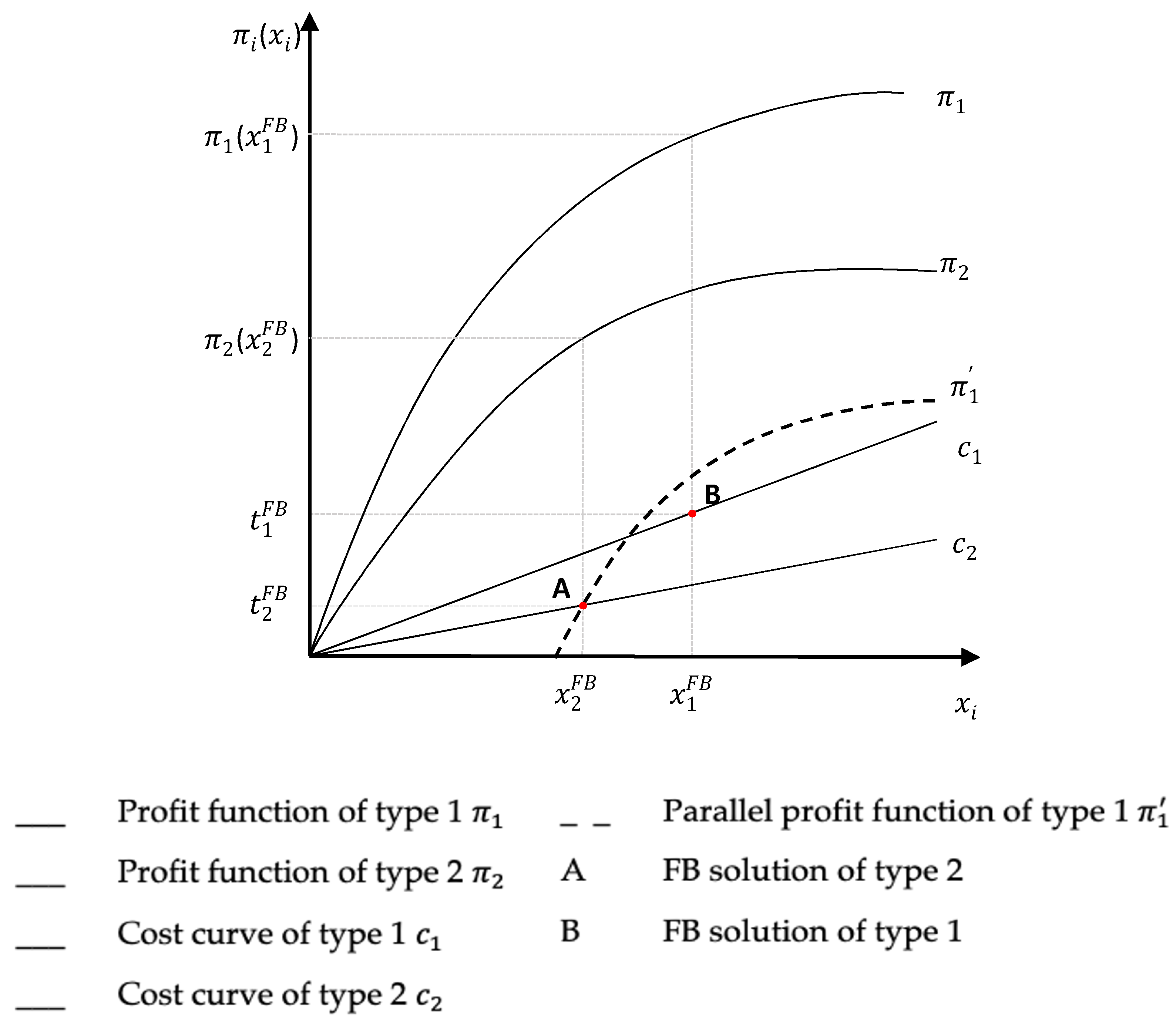
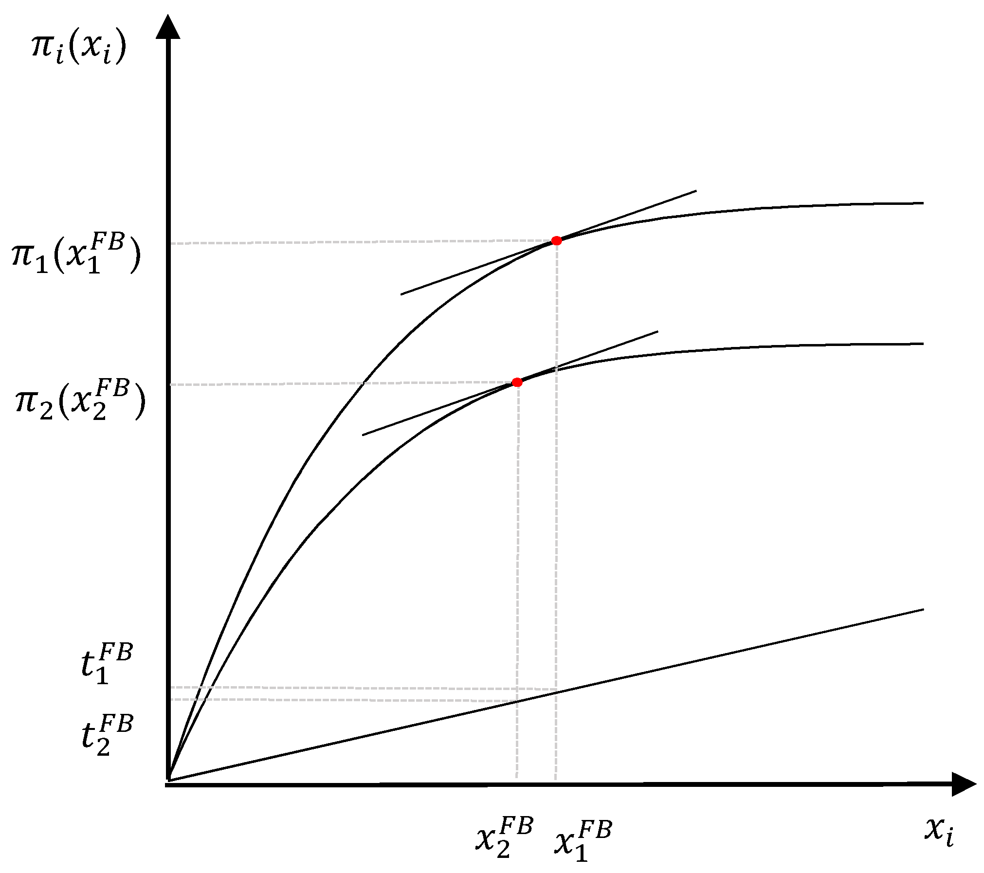
First, we consider the case in which the difference between cost functions with respect to farm types is smaller than the difference between profit functions (i.e., $c_1\left(x_1\right)-c_2\left(x_2\right)<{\pi }_1\left(x_1\right)-{\pi }_2\left(x_2\right))$. We show that, under these conditions, the first-best itself is still incentive-compatible for some combination of profit and cost functions due to the (small) distance between the two cost functions. Figure 1 illustrates this case. In the figure, ${\pi }_1$ indicates the profit curve for farm type 1, which is steeper than that for type two ${\pi }_2$ in each point. The cost line $c_1$ belongs to farm type 1 and is higher than the one belonging to type 2, $c_2$. The red point A on the cost function of type 2 indicates the first-best solution for type 2; the same applies to point B for type 1. From the assumptions above, we expect that type 1 behaves truthfully because it can obtain a higher profit (vertical distance between the profit and cost function at point (B) by paying a higher tariff $t_1$ and by benefiting from irrigating a higher share allowed by this contract.

By drawing the parallel profit function of type 1 ${\pi }_1^{\prime }$ (efficient) passing through point A, it is evident that type 1 is not interested in selecting the contract addressed to the other farm type because the cost saving achieved by selecting that contract is lower than the corresponding loss of profit that he/she would face by reducing the irrigated share. This is shown from the profit curve that passes above the red point B, which is the solution designed for farm type 1 in the first-best and point A belonging to the solution of type 2 (i.e., while the distance between profit and cost is always higher in $x_1^{FB}$ than in $x_2^{FB}$). As a result, the first-best solution still holds for farm type 1. The same can be shown for farm type 2, so first-best contract solutions still hold, i.e., are incentive-compatible.

In the second case, let us continue to assume the properties of profit and cost functions of the example above and examine a case in which the difference in the cost function is large compared with the difference in the profit function. Under this assumption, a farmer might have an incentive to cheat, hence creating a problem of adverse selection.

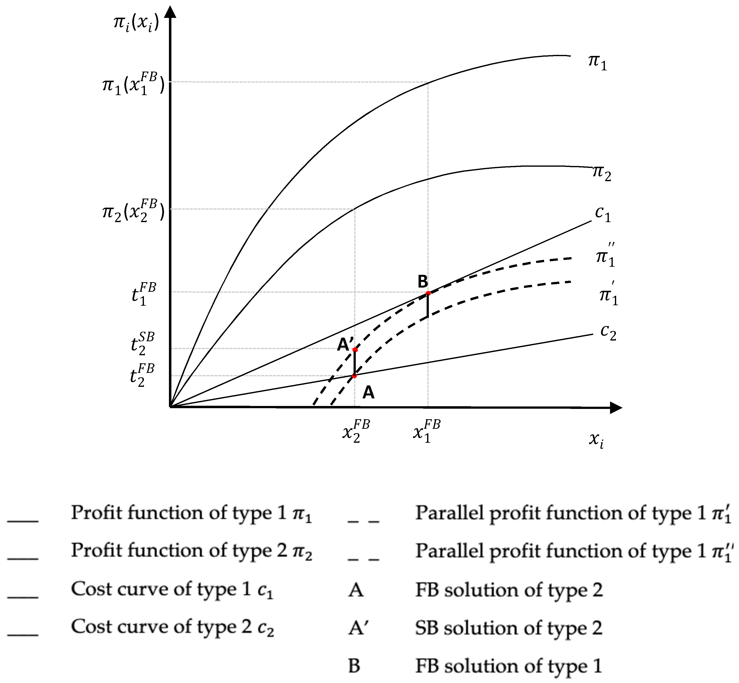
The illustration of the solution is supported by a graphical interpretation in Figure 2, which shows that the difference in the cost function is higher than the one considered in Figure 1. This difference is described by the distance of the parallel in the profit function ${\pi }_1^{\prime }$, drawn through point A, which indicates the first-best solution of type 2, with the solution for type 1, point B, illustrated by the vertical bold black line (i.e., from ${\pi }_1^{\prime }$ to B). In this case, the first-best solution is not incentive-compatible anymore as it is in the interest of farm type 1 to mimic farm type 2. The farmers act opportunistically in order to maximize profits; type 1 chooses the contract designed for type 2 because the combination of tariffs and irrigated share of type 2 ensure a higher profit. Therefore, another strategy needs to be pursued by the WA by way of mechanism design.

In order to induce each farm to choose the contract designed for it and considering no transaction costs (from the money transfer), the best option to optimize the problem is to increase the water tariff for farm type 2. The tariff increase is in the form of an additional payment compared to the first-best to disincentivize the selection of the wrong contract by type 1. This increase is described by the vertical black bold line illustrating the distance from point A to A’. The tariff increase is at least up to the level that equalizes the distance between the ${\pi }_1^{\prime }$ curve and red point B. This is illustrated by drawing another parallel of the profit curve of farm type 1, indicated by ${\pi }_1^{″}$ passing through the point belonging to the second-best solution of type 2 (point A’). With this tariff increase for the contract designed for farm type 2, farm type 1, potentially cheating, remains indifferent with regard to the two contract types as the option to cheat will not make the farmer better off. The second-best tariff in the contract solution is, in the first instance, the one illustrated by point B for farm type 1 (the same as in the first-best) and point A’ for type 2 (unlike in the first-best case). The optimal shares of irrigated land do not change compared with first-best if the tariff does not entail any transaction costs and is only a transfer of money.

This analysis allows us to conclude that the first-best solution is also achievable under asymmetric information but only in cases where the cost functions (with respect to profits) are sufficiently close between types or when there are no transaction costs for monetary transfers. In the latter case, the first-best share of irrigated land is achieved by simply modifying the level of tariffs. The latter assumption is revised in the next case.

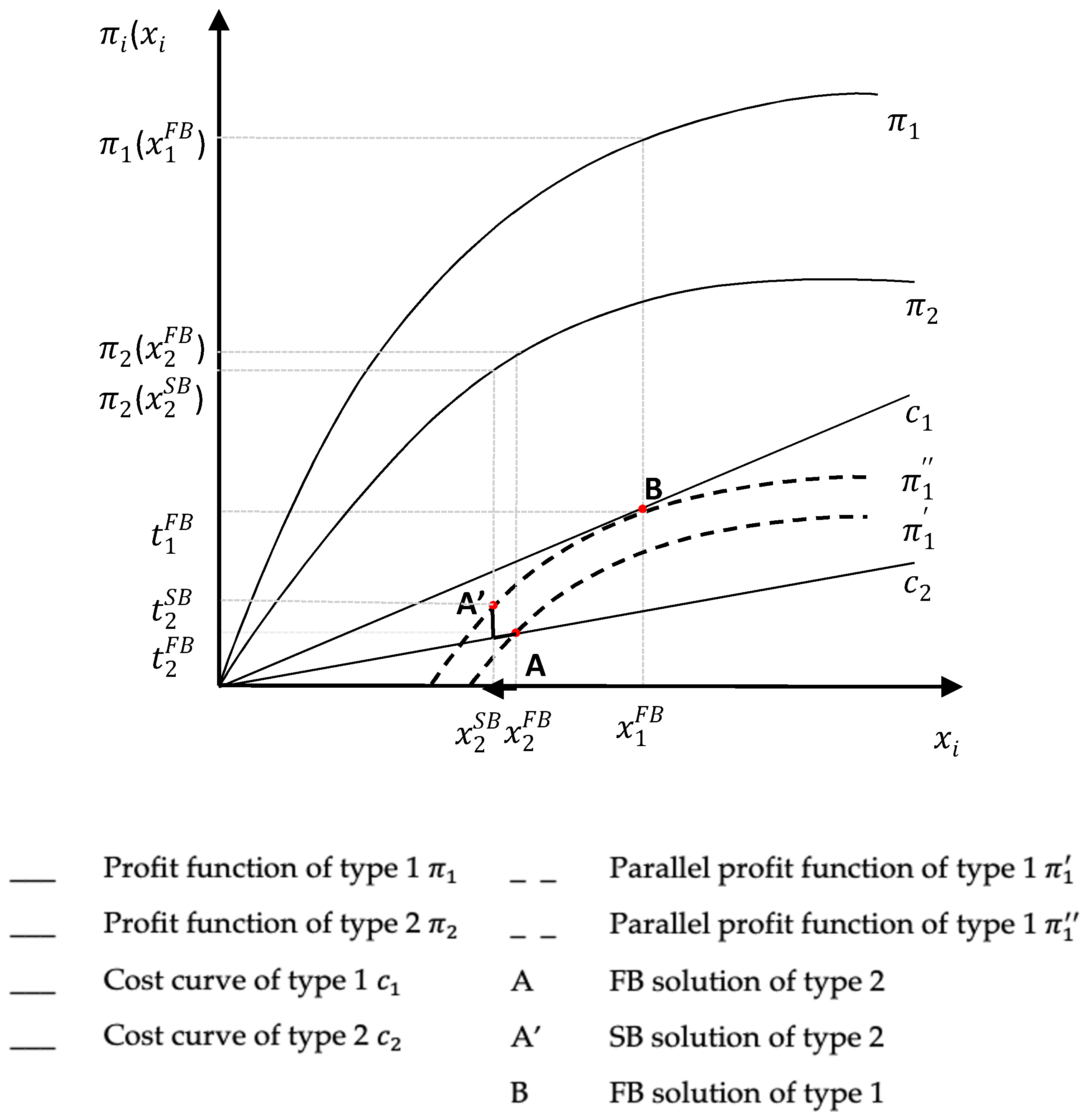
In the third case, we make the hypothesis that the properties of the profit and cost functions are still the same as in the case above, but it is assumed that the WA faces positive transaction costs from farms’ money transfers for the additional payments provided to farmers to ensure that farmers reveal their types. As transaction costs are set linear on tariffs and incorporated into farms’ tariffs to ensure that cost recovery also recovers transaction costs, the final tariffs paid by farmers will further increase. However, it is now optimal for the WA to consider a decrease in the irrigated share of type 2 instead of just increasing the tariff in order to moderate the additional transaction costs. The result is shown in Figure 3. The solution under this assumption is illustrated by the black lines drawn from point A to A’ and the decrease in the irrigated share of type 2 from $x_2^{FB}$ to $x_2^{SB}$. This move is associated with the establishment of a new level of water tariffs from $t_2^{FB}$ to $t_2^{SB}$ for type 2 and $t_1^{FB}$ = $t_1^{SB}$ for type 1.

The second-best solution is determined at point B for farm type 1 and A’ for type 2. Note that the decrease in the irrigated share from $x_2^{FB}$ to $x_2^{SB}$ eventually corresponds to a decrease in the profits of farm type 2 from ${\pi }_2^{FB}\left(x_2^{FB}\right)$ to ${\pi }_2^{SB}\left(x_2^{SB}\right)$ while the profits of farm type 1 do not change as the irrigated share for farm type 1 has not changed.

Formally, in the second-best, $C{R}_1$ and $I{C}_1$ are binding with strict equality. Maximizing the objective function subject to binding constraints with $v>0,$ the following solution is achieved:

$${\pi }_1^{\prime }\left(x_1^{FB}\right)=\frac{c_1^{\prime }\left(x_1^{FB}\right)}{1-v},$$

(15)

$${\pi }_2^{\prime }\left(x_2^{SB}\right)=\frac{c_2^{\prime }\left(x_2^{SB}\right)}{1-v}+\frac{v}{1-v}[{\pi }_1^{\prime }\left(x_2^{SB}\right)-{\pi }_2^{\prime }\left(x_2^{SB}\right)],$$

(16)

The solution indicates that the contract designed for the efficient farm type is the same as in the first-best while the contract designed for the inefficient farm type reveals a distortion in the irrigated share, which is different from the cases considered above. Comparing the solution in Equation (16) with the one in Section 4.2.3 for the inefficient farm type, it can be observed that the inefficient farm receives a more costly contract. This result occurs due to the increase in the water tariff (see Figure 3) and due to the lower irrigated share. The quota of irrigated share $x_2^{SB}$ is determined by solving Equation (16). From the right-hand side of Equation (16), it is shown that the marginal cost of type 2 is greater than the one found in Section 4.2.3 because of the positive difference in the last part of the equation (as, by assumption, the marginal profits of type 1 are greater than type 2). From the properties of the cost function, this increase in the marginal cost eventually corresponds to a lower irrigated share, represented by $x_2^{SB}$ (i.e., as illustrated in Figure 3).

One might ask why the regulator does not prefer to adjust $t_1$. However, if the regulator decreases $t_1$ to make IC₁ or IC₂ binding, they violate CR₁ by setting water tariffs at a level that is below cost. On the other hand, if the regulator increases $t_1$, CR₁ does not bind, becoming strictly greater than the costs and (from Figure 3) further incentivizes type 1 to choose the wrong contract.

The main result of this analysis is that the distance between profits and cost functions are fundamental in designing appropriate incentive contract solutions and that the chosen mechanism needs to be carefully designed to avoid any efficiency loss and, at the same time, to exploit the opportunities provided by costs/profits configurations.

5. Discussion

This paper provides a formal analysis of incentive water pricing policies in irrigated agriculture. The mechanism design refers to a case where irrigation water is supplied through open canals and is unmetered. The study considers a principal-agent model that allows the WA to develop pricing strategies aimed at maximizing social benefits. The paper further develops the model used in Lika et al. [18].

This is also the only paper that, strictly speaking, is comparable to this one. Our results are consistent with the empirical results by Lika et al. [18]; however, in our model, the costs here are assumed to be linear and are analysed with a broader set of assumptions. This allows us to identify a set of general cases that can be used in a more straightforward way for policy prescriptions. Here, we also consider more explicitly the role of incentive constraints, transaction costs and cost recovery constraints.

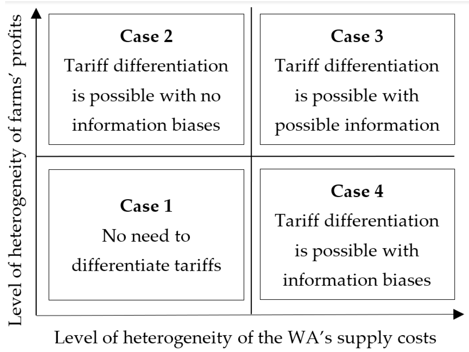
One lesson learned from the insights above is that incentive pricing in different contexts can be more or less efficient and desirable from a social point of view. The practicability of incentive pricing strategies in the absence of water metering depends on the existence of suitable proxies of water use to design pricing schemes, such as tariffs proportional to the share of irrigated area, and on the potential improvement of the “allocative” efficiency, which is linked to farm heterogeneity including in terms of costs and profits. The impact of heterogeneity on the optimal tariff design option is illustrated in Figure 4 by showing how different combinations of profits and costs fit with pricing policies. We identify four cases.

• Farms are homogeneous both in profits and costs. Under these conditions, there is no need to provide an incentive strategy to differentiate tariffs because the costs of guaranteeing price discrimination might not be justified compared with the benefit from differentiation. With such a hypothesis, the regulator can simply apply a flat rate or, better, a tariff proportional to the irrigated area without applying a more complex incentive pricing strategy.
• Farms are heterogeneous in profits but not in costs. Under this condition, the adverse selection problem will occur and the WA will impose tariff differentiation only if the efficiency gain by differentiating is higher than the costs arising from the implementing incentive strategy.
• Farmers are heterogeneous in profits and in costs. The existence of different supply costs among farm types provides the motivation to verify the possibility of differentiating tariff options in such a way as to encourage farmers to self-qualify through the choice of the contract. This possibility is influenced by the level of transaction costs faced to implement such a tariff option and by the additional cost imposed on farmers to ensure incentive-compatible contract design to face adverse selection. This cost decreases with increasing differences in profits among efficient and inefficient farm types.
• Farms are heterogeneous in costs but not in profits. If the population of farmers is located on the lower right of the figure, the WA faces an adverse selection problem. This requires the design of suboptimal contracts, including the provision of incentives, which means the pricing policy is more costly than it would be in conditions of perfect information. This option is extensively analysed above, where the achievement of efficient solutions depends on the degree of heterogeneity among farmers and transaction cost levels.

Overall, as a result of this discussion, it can be concluded that the ability to implement incentive pricing depends on (1) the characteristics of the irrigation network that affects the implementation costs (direct transaction costs); (2) the characteristics of the community of farmers served by the network that affects the economic losses caused by the presence of information biases between principals and agents (indirect transaction costs); and (3) the identification of priorities motivating the implementation of incentive mechanisms by the WA (policy, environmental and equity issues).

Several limitations do exist for this study. An important limitation is the approximation of farm water use through an irrigated share of farmland, i.e., irrigated share assumed as a proxy of water use. The use of proxy measures is considered a limitation because of imperfect estimates of water demand. Actually, the paper precisely addresses the issue that measuring irrigated area cannot fully account for the information about water use (the area can be measured and this is needed to have it as part of the contract, but it remains unknown how it relates to costs and profits for each individual farmer). However, different and better proxies can be identified.

Another limitation can be found in the fact that we considered the effect of an adverse selection problem in the presence of information asymmetries between the WA and the farmers whilst not considering the presence of the moral hazard.

Also, we left aside the effect of climate change on the water supply and ultimately its effects on water costs and the consequent implication for designing pricing schemes. As climate change is one of the main drivers of current adaptations, this could be a priority topic to be addressed in further research.

Moreover, we assumed that transaction costs are simply proportional to water tariffs when there might also be a fixed and nonlinear variable component that contributes to further complicating the WA’s incentive pricing policy. Certainly, there may be other cases in which transaction costs differ in their form and among types.

In addition, in our analysis, we did not explicitly discuss compatibility with the Polluter Pays Principle (PPP), a very important issue for water policy. Knowing that PPP is closely interlinked with the other two principles (Incentive Pricing Policies (IPP) and Cost Recovery (CR)) [42] by means of incentive pricing policy designs in this study, it is possible to boost rational water uses that might contribute to softening related negative environmental effects. However, direct interlinkages with PPP are out of the scope of this paper but could be further investigated.

However, our model can be expanded to consider these costs related to PPP by simply including them in the WA’s cost for water delivery to farmers ($c_i\left(x_i\right)$). However, as environmental and resource costs may have different behaviours (both because they follow different functional forms with respect to water abstraction and because they often have the nature of public goods), it would be preferable to work with them through a different item of the objective function and potentially a different constraint in future developments of this model.

Other limitations are related to the fact that we consider a limited set of hypotheses of combinations of profit and cost functions. For example, assuming a quadratic cost function in the modelling approach could lead to different results from the ones introduced thus far. Addressing these issues could be considered in future research.

6. Conclusions

The provision of water resources through open canals and the potential inefficiencies in its use by farmers under flat rate pricing motivates research on the design of alternative pricing strategies that provide incentives for the rational use of water resources according to the WFD requirements, IPP and CR.

The mechanism design for incentive pricing, overall, matches two of the requirements of Article 9 of the Directive 2000/60/EC [4]. The IPP is addressed by developing an incentive strategy that connects farms’ water tariffs (indirectly) with the farms’ water uses. In addition, water tariffs cover water supply costs and associated transaction costs (i.e., cost recovery).

Through our analysis, we demonstrate that incentive pricing options are possible even under asymmetric information conditions, though the related efficiency gains and losses are highly case specific. By separating hypotheses about costs and profit functions, we also show that first-best incentive contracts can be implemented even under asymmetric information, in particular, when differences in costs for water use are small compared to differences in irrigation profits across farms and/or when transaction costs related to tariff implementation are low.

The main policy prescription remains that incentive pricing strategies via menus of contracts need to be designed in such a way that the features of each particular region are taken into consideration. On the other hand, the feasibility of these contract solutions may be greater than usually expected, even when water is not measured. This can include first-best solutions that are not just theoretical options but can actually be the best solution for a class of real-life situations. In order to exploit these opportunities, the policy would need to be more carefully designed, taking into account farmers’ heterogeneity and incentive compatibility.

An obvious extension of this methodology could be in the direction of an empirical application. In addition, the investigation of the joint problem of adverse selection and moral hazard in irrigated agriculture might be a further step forward as a way of bringing models closer to a realistic assessment of the economic efficiency of different policy instruments. Another potential extension of this method (alone or combined with those listed above) could be an assessment of the effects of different transaction cost structures (fixed and variable transaction costs) on optimal policy design.

References

- Haavisto, R.; Santos, D.; Perrels, A. Determining payments for watershed services by hydro-economic modeling for optimal water allocation between agricultural and municipal water use. Water Resour. Econ. 2019, 26, 1–17. Available online: http://repositorio.senamhi.gob.pe/bitstream/handle/20.500.12542/40/1-s2.0-S2212428417300877-main.pdf?sequence=1&isAllowed=y (accessed on 27 July 2020). [CrossRef]
- Expósito, A. Irrigated agriculture and the cost recovery principle of water services: Assessment and discussion of the case of the guadalquivir river basin (Spain). Water 2018, 10, 1338. [Google Scholar] [CrossRef] [Green Version]
- OECD. Sustainable Management of Water Resources in Agriculture; OECD Publishing: Paris, France, 2010; Available online: http://www.oecd.org/greengrowth/sustainable-agriculture/49040929.pdf (accessed on 27 July 2020).
- European Commission. “Directive 2000/60/ec of the European Parliament and of the Council of 23 October 2000 Establishing a Framework for Community Action in the Field of Water Policy”. Available online: https://eur-lex.europa.eu/resource.html?uri=cellar:5c835afb-2ec6-4577-bdf8-756d3d694eeb.0004.02/DOC_1&format=PDF (accessed on 27 July 2020).
- Toan, T.D. Water pricing policy and subsidies to irrigation: A review. Environ. Process. 2016, 3, 1081–1098. [Google Scholar] [CrossRef]
- European Environment Agency. Assessment of Cost Recovery through Water Pricing; Luxembourg Publications Office: Brussels, Belgium, 2013; Available online: https://www.google.com/search?client=safari&rls=en&q=European+Environment+Agency,+Assessment+of+cost+recovery+through+water+pricing.+Luxembourg:+Publications+Office,+2013&ie=UTF-8&oe=UTF-8 (accessed on 27 July 2020).
- Easter, K.W.; Liu, Y. Cost recovery and water pricing for irrigation and drainage projects. Agriculture and rural development discussion paper 26. In The International Bank for Reconstruction and Development; The World Bank: Washington, DC, USA, 2005. [Google Scholar]
- Lika, A.; Galioto, F.; Viaggi, D. Water authorities’ pricing strategies to recover supply costs in the absence of water metering for irrigated agriculture. Sustainability 2017, 9, 2210. [Google Scholar] [CrossRef] [Green Version]
- Galioto, F.; Raggi, R.; Viaggi, D. Assessing the potential economic viability of precision irrigation: A theoretical analysis and pilot empirical evaluation. Water 2017, 9, 990. [Google Scholar] [CrossRef] [Green Version]
- Expósito, A.; Berbel, J. Why is water pricing ineffective for deficit irrigation schemes? A case study in southern spain. Water Resour. Manag. 2017, 31, 1047–1059. [Google Scholar] [CrossRef]
- Dinar, A. Policy implications from water pricing experiences in various countries. Water Policy 1998, 1, 239–250. [Google Scholar] [CrossRef]
- Bartolini, F.; Bazzani, G.M.; Gallerani, V.; Raggi, M.; Viaggi, D. The impact of water and agriculture policy scenarios on irrigated farming systems in Italy: An analysis based on farm level multi-attribute linear programming models. Agric. Syst. 2007, 93, 90–114. [Google Scholar] [CrossRef]
- Martin-Ortega, A.J.; Skuras, D.; Perni, A.; Holen, S.; Psaltopoulos, D. The disproportionality principle in the WFD: How to actually apply it. In Economics of Water Management in Agriculture; Thomas, B., Julio, B., Basil, M., Davide, V., Eds.; Science Publishers: Enfield, NH, USA, 2015; pp. 214–249. [Google Scholar]
- Bogaert, S. The Role of Water Pricing and Water Allocation in Agriculture in Delivering Sustainable Water Use in Europe—Final Report; Arcadis: Brussels, Belgium, 2012. [Google Scholar]
- Galioto, F.; Raggi, M.; Viaggi, D. Pricing policies in managing water resources in agriculture: An application of contract theory to unmetered water. Water 2013, 5, 1502–1516. [Google Scholar] [CrossRef]
- Irrigation Water Pricing: The Gap between Theory and Practice; Molle, F.; Berkoff, J. (Eds.) CABI: Wallingford, UK; Cambridge, MA, USA, 2007; Available online: https://horizon.documentation.ird.fr/exl-doc/pleins_textes/divers16-09/010045237.pdf (accessed on 27 July 2020).
- Molle, F.; Venot, J.P.; Hassan, Y. Irrigation in the jordan valley: Are water pricing policies overly optimistic? Agric. Water Manag. 2008, 95, 427–438. [Google Scholar] [CrossRef]
- Lika, A.; Galioto, F.; Scardigno, A.; Zdruli, P.; Viaggi, D. Pricing unmetered irrigation water under asymmetric information and full cost recovery. Water 2016, 8, 596. [Google Scholar] [CrossRef] [Green Version]
- Molle, F. Water scarcity, prices and quotas: A review of evidence on irrigation volumetric pricing. Irrig. Drain. Syst. 2009, 23, 43–58. [Google Scholar] [CrossRef]
- Viaggi, D.; Raggi, M.; Bartolini, G.; Gallerani, V. Designing contracts for irrigation water under asymmetric information: Are simple pricing mechanisms enough? Agric. Water Manag. 2010, 97, 1326–1332. [Google Scholar] [CrossRef]
- Johansson, R. Pricing irrigation water: A review of theory and practice. Water Policy 2002, 4, 173–199. [Google Scholar] [CrossRef]
- Smith, R.B.W.; Tsur, Y. Asymmetric information and the pricing of natural resources: The case of unmetered water. Land Econ. 1997, 73, 392. [Google Scholar] [CrossRef]
- Akerlof, G.A. The market for ‘lemons’: Quality uncertainty and the market mechanism. Q. J. Econ. 1970, 84, 488–500. Available online: https://econpapers.repec.org/article/oupqjecon/v_3a84_3ay_3a1970_3ai_3a3_3ap_3a488-500..htm (accessed on 31 July 2020). [CrossRef]
- Mirrlees, J.A. An exploration in the theory of optimum income taxation. Rev. Econ. Stud. 1971, 38, 175–208. [Google Scholar] [CrossRef]
- Spence, M. Job market signaling. Q. J. Econ. 1973, 87, 355. [Google Scholar] [CrossRef]
- Stiglitz, J. The theory of ‘screening,’ education, and the distribution of income”. Am. Econ. Rev. 1975, 65, 283–300. Available online: https://www.jstor.org/stable/1804834?seq=1 (accessed on 27 July 2020).
- Rothschild, M.; Stiglitz, J. Equilibrium in competitive insurance markets: An essay on the economics of imperfect information. In Uncertainty in Economics; Academic Press: Cambridge, MA, USA, 1976; pp. 257–280. [Google Scholar]
- Laffont, J.J.; Martimort, D. The rent extraction-effciency trade-off. In Theory of Incentives: The Principal-Agent Model; Princton University Press: Princton, NJ, USA, 2002. [Google Scholar]
- Hurwicz, L. Optimality and Informaational Effciency in Resourc Allocation Processes; Stanford University Press: Palo Alto, CA, USA, 1960. [Google Scholar]
- Harsanyi, J.C. Games with incomplete information played by ‘Bayesian’ players, I-III. Manag. Sci. 1967, 14, 159–182. Available online: http://www.dklevine.com/archive/refs41175.pdf (accessed on 27 July 2020). [CrossRef]
- Fudenberg, D.; Tirole, J. Game Theory, 1st ed.; The MIT Press: Cambridge, MA, USA, 1991. [Google Scholar]
- Gallerani, V.; Raggi, M.; Viaggi, D. Irrigation water pricing and cost recovery under asymmetric information. Water Sci. Technol. 2005, 5, 189–196. [Google Scholar] [CrossRef]
- Berbel, J.; Borrego-Maria, M.M.A.; Expósito, A.; Giannoccaro, G.; Montilla-Lopez, M.N.; Roseta-Palma, C. Analysis of irrigation water tariffs and taxes in Europe. Water Policy 2019, 21, 806–825. [Google Scholar] [CrossRef] [Green Version]
- Tsur, Y.; Dinar, A.; Doukkali, R.M.; Roe, L.T. Irrigation water pricing: Policy implications based on international comparison. Environ. Dev. Econ. 2004, 9, 735–755. [Google Scholar] [CrossRef] [Green Version]
- Cornish, G.; Bosworth, B.; Perry, C.J.; Burke, J.J. Water Charging in Irrigated Agriculture: An Analysis of International Experience; Food and Agriculture Organization of the United Nations: Rome, Italy, 2004. [Google Scholar]
- Franco-Crespo, C.; Viñas, S.J. The impact of pricing policies on irrigation water for agro-food farms in ecuador. Sustainability 2017, 9, 1515. [Google Scholar] [CrossRef] [Green Version]
- Latinopoulos, D. Derivation of irrigation water demand functions through linear and non-linear optimisation models: Application to an intensively irrigated area in northern Greece. Water Sci. Technol. 2005, 5, 75–84. [Google Scholar] [CrossRef]
- Zhang, L.; Heerink, N.; Dries, L.; Shi, X. Water users associations and irrigation water productivity in northern China. Ecol. Econ. 2013, 95, 128–136. [Google Scholar] [CrossRef] [Green Version]
- Arguedas, C.; van Soest, D.P. Optimal conservation programs, asymmetric information and the role of fixed costs. Environ. Resour. Econ. 2011, 50, 305–323. [Google Scholar] [CrossRef] [Green Version]
- Fjell, K. A cross-subsidy classification framework. J. Public Policy 2011, 21, 265–282. [Google Scholar] [CrossRef]
- Qtaishat, H.T.; El-Habbab, S.M.; Bumblauskas, P.D. Welfare economic analysis of liftingwater subsidies for banana farms in jordan. Sustainability 2019, 11, 5118. [Google Scholar] [CrossRef] [Green Version]
- Grossman, R.M. Agriculture and the polluter pays principle. Electron. J. Comp. Law 2007, 54, 317–339. Available online: http://www.ejcl.org/113/article113-15.pdf (accessed on 27 July 2020).
Figure 1.
Illustration of the first-best solution under asymmetric information.
Figure 2.
Illustration of the second-best solution under asymmetric information: the pricing effect.
Figure 3.
Illustration of the second-best solution under asymmetric information: the combined pricing and irrigated share effects.
Figure 4.
The impact of heterogeneity on pricing design options.
© 2020 by the authors. Licensee MDPI, Basel, Switzerland. This article is an open access article distributed under the terms and conditions of the Creative Commons Attribution (CC BY) license (http://creativecommons.org/licenses/by/4.0/).
Share and Cite
MDPI and ACS Style
Viaggi, D.; Galioto, F.; Lika, A. The Design of Pricing Policies for the Management of Water Resources in Agriculture Under Adverse Selection. Water 2020, 12, 2174. https://doi.org/10.3390/w12082174
AMA Style
Viaggi D, Galioto F, Lika A. The Design of Pricing Policies for the Management of Water Resources in Agriculture Under Adverse Selection. Water. 2020; 12(8):2174. https://doi.org/10.3390/w12082174
Chicago/Turabian StyleViaggi, Davide, Francesco Galioto, and Alban Lika. 2020. "The Design of Pricing Policies for the Management of Water Resources in Agriculture Under Adverse Selection" Water 12, no. 8: 2174. https://doi.org/10.3390/w12082174
Note that from the first issue of 2016, this journal uses article numbers instead of page numbers. See further details here.