Spectral Decomposition of X-ray Absorption Spectroscopy Datasets: Methods and Applications


1
Department of Chemistry, NIS Center and INSTM Reference Center, University of Turin, via P. Giuria 7, 10125 Turin, Italy
2
The Smart Materials Research Institute, Southern Federal University, Sladkova 178/24, 344090 Rostov-on-Don, Russia
*
Authors to whom correspondence should be addressed.
Crystals 2020, 10(8), 664; https://doi.org/10.3390/cryst10080664
Submission received: 17 June 2020
/
Revised: 16 July 2020
/
Accepted: 17 July 2020
/
Published: 1 August 2020
(This article belongs to the Special Issue Multivariate Analysis Applications to Crystallography)
Abstract
:X-ray absorption spectroscopy (XAS) today represents a widespread and powerful technique, able to monitor complex systems under in situ and operando conditions, while external variables, such us sampling time, sample temperature or even beam position over the analysed sample, are varied. X-ray absorption spectroscopy is an element-selective but bulk-averaging technique. Each measured XAS spectrum can be seen as an average signal arising from all the absorber-containing species/configurations present in the sample under study. The acquired XAS data are thus represented by a spectroscopic mixture composed of superimposed spectral profiles associated to well-defined components, characterised by concentration values evolving in the course of the experiment. The decomposition of an experimental XAS dataset in a set of pure spectral and concentration values is a typical example of an inverse problem and it goes, usually, under the name of multivariate curve resolution (MCR). In the present work, we present an overview on the major techniques developed to realize the MCR decomposition together with a selection of related results, with an emphasis on applications in catalysis. Therein, we will highlight the great potential of these methods which are imposing as an essential tool for quantitative analysis of large XAS datasets as well as the directions for further development in synergy with the continuous instrumental progresses at synchrotron sources.
1. Introduction
One of the main dreams for researchers working in the field of chemistry consists in identifying analytical tools which allow one to obtain an atomic-scale movie of a chemical reaction under realistic working conditions [1]. This ultimate target requires the simultaneous determination of characteristic (spectroscopic, diffractometric, etc.) signatures and concentrations of all the species involved in the analysed process (i.e., reactants, intermediates and products) monitored by one or more characterisation methods as a function of time or any other variable controlled within the experiment. In this way, a reliable correlation between structure, kinetics and functionality can be properly identified.
With an emphasis on the field of catalysis, X-ray absorption spectroscopy (XAS) demonstrated to be an extremely powerful technique, principally thanks to its local sensitivity and element selectivity, together with the possibility to simultaneously access both electronic and structural information of the material under study [2,3,4].
X-ray absorption spectroscopy measures the X-ray absorption coefficient μ(E) of the sample as a function of the energy E of the incident X-ray beam, in the proximity of an absorption edge (at energy E0) for one of the elements present in the sample, indicated as the absorber. For XAS experiments, an incident X-ray beam with continuously tunable energy together with a high photon flux to achieve satisfactory data quality are needed; these requirements almost exclusively render XAS a synchrotron-based technique. The X-ray absorption near edge structure (XANES) region of a XAS spectrum covers a few tens of eV before and after the edge. The XANES spectrum mainly reflects the unoccupied electronic levels of the absorber and contains a number of spectral fingerprints enabling an accurate determination of the absorber oxidation state, coordination geometry and symmetry [5,6,7]. The extended X-ray absorption fine structure (EXAFS) region encompasses the spectral range at higher energies, starting from the end of the XANES region and typically extending up to 1 keV after the edge. Here, if the absorber is surrounded by atomic neighbours, the smoothly decreasing μ0(E) atomic absorption background is modulated by subtle oscillations. This fine structure originates from the interference among wave-fronts back-scattered by the different shells of atomic neighbours surrounding the absorber, after the ejected photoelectron has diffused as a spherical wave [8].
The EXAFS function χ(k), obtained after “extraction” of the oscillatory part of μ(E) and expressed as a function of the photoelectron wavenumber k = (1/ħ) [2me(E − E0)]1/2 (where me is the electron mass) can be related to a specific radial arrangement of the atomic neighbours in the local environment of the absorber, with the aid of Fourier transform (FT) to bridge the photoelectron wavenumber space (k-space) to the direct R-space [2,3,4,9,10]. Fitting of the EXAFS signal based on the so-called the EXAFS equation [8] offers the possibility to quantitatively refine local structural parameters for each coordination shell including average interatomic distances, coordination numbers and types of atomic neighbours and Debye-Waller (DW) factors accounting for thermal vibrations and static structural disorder. The short photoelectron mean free path in matter and the damping effect of the core-hole lifetime limits EXAFS sensitivity to a sphere of 5–10 Å radius from the absorber, thus determining the local character of the technique.
X-ray absorption spectroscopy is an element selective but average technique. The XAS signal exclusively stems from the absorber-containing species in the system, but it is averaged over all such species simultaneously present in the sample volume probed by the X-ray beam, weighted by their relative abundance. On the one hand, element selectivity represents a key advantage in the field of catalysis, especially for the characterisation of heterogeneous catalysts where highly diluted active sites are often distributed without long-range order over a much more abundant (crystalline or amorphous) support/matrix [2,11,12,13]. On the other hand, the average response of the technique poses important challenges in situations where multiple absorber-containing species (e.g., active and inactive/spectator species) coexist and dynamically evolve along the experiment. This is most often the case during in situ/operando studies of catalysts, nowadays representing the golden standard for characterisation in the field.
This review focuses on statistical approaches and spectral decomposition methods applied to robustly resolve the different contributions within a XAS dataset, aimed at overcoming the interpretative limitations connected with the average nature of the XAS technique. While the earlier efforts in this direction date back to the 1990s [14], the last few years have seen a rapid boost in their use [7,15,16], naturally connected with the continuous instrumental developments at synchrotron sources. Nowadays, outstanding time-resolution in XAS data collection can be achieved, even on diluted samples under reaction-relevant conditions, spanning from few minutes on conventional XAS beamlines, to few seconds and down to the (sub)ms-time scale using high-energy resolution off-resonant spectroscopy (HEROS) [17,18] as well as quick [19] and dispersive XAS setups [20]. The increasingly larger datasets generated in such experiments (in the order of 103–104 scans) urgently claim for appropriate data management and analysis tools, embracing chemometrics and emerging machine learning (ML) implementations [21].
Herein, in Section 2, we provide a step-by-step overview on the key mathematical methods and models required to approach this intriguing and rapidly growing field. We start from principal component analysis (PCA), an indispensable tool to identify the number of components effectively contributing in the analysed dataset. Then, we clarify the taxonomy of the main spectral decomposition methods yielding physico-chemically meaningful spectral and concentration profiles for the identified pure components, from methods requiring a priori spectroscopic/kinetic knowledge of the investigated system to multivariate curve resolution (MCR) approaches enabling the so-called blind source separation. For each method, we critically discuss strengths and weaknesses with an emphasis on its application to XAS data analysis.
To date, XAS spectral decomposition methods have been successfully employed in a large variety of research fields; recent examples encompass solid-state physics and chemistry [22,23,24], energy-storage materials [25,26,27,28,29], environmental science [30], homogeneous [31,32] and heterogeneous catalysis [15,33,34,35,36,37,38,39,40,41,42,43]. While an exhaustive review of the available literature falls beyond the scope of this work, in Section 3, we present a selection of examples in catalysis, corroborating the general information discussed in Section 2. The selected case studies are organized around two important classes of heterogeneous catalysts, namely, metal-exchanged zeolites and supported metal catalysts, highlighting the potential of PCA coupled with various spectral decomposition methods in resolving the spectral mixture for these structurally challenging and highly dynamic systems studied by in situ/operando XAS.
A final summary is reported in Section 4, together with a critical assessment of the main areas, where we envisage the most exciting developments of the relevant methods to take place in the forthcoming future, taking us a step closer to the dream of unblurred atomic-scale movies of chemical reactions.
2. Methods for XAS Spectral Decomposition
When a sample consists of a mixture of absorbing atoms forming different chemical species or located in non-equivalent sites, the related XAS measurement represents an average of the single spectra corresponding to each species/site. It is worth noting that the XAS spectral features associated to a given absorbing atom will depend exclusively on the local geometry of the related species/site. This fact leads to the conclusion that the XAS spectra of each species characterising the sample measurement, will be different to each other and, for this reason, they can be defined as pure spectra. It follows that an arbitrary XAS spectrum can be expressed as the sum of these pure spectra weighted by their amount inside the sample:
Here, N is the number of pure spectral compounds involved in the decomposition, is the energy vector, is the energy dependent pure spectrum corresponding to the ith species/site, is a scalar value representing the fractional abundance or concentration of inside the sample under study, while is a vector containing experimental noise values associated to the measure. Because of the element-selectivity of the XAS technique, it is possible to assert that, in general, the mass balance condition must be satisfied: .
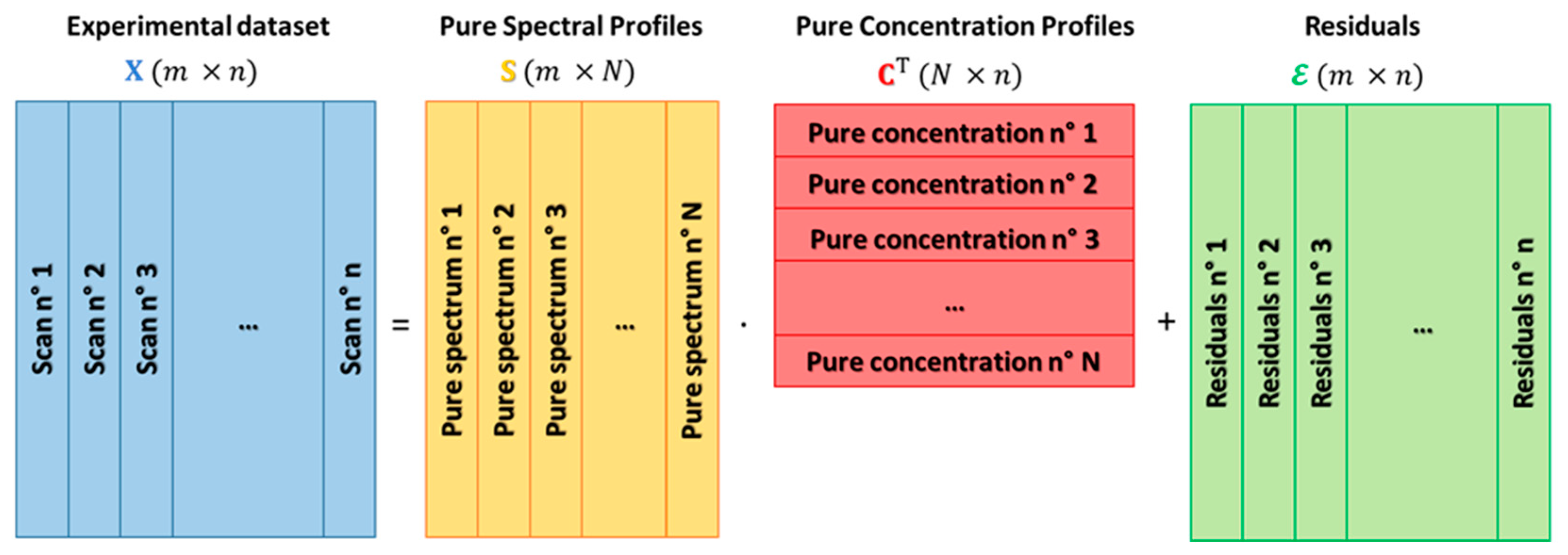
Equation (1) can be extended to the case of a dataset containing multiple spectra collected during the variation of the physico-chemical system under study, caused by the controlled modification of one or more external factors (e.g., temperature, gas feed composition, sampling time, sample position, etc.):
where is composed of energy points and spectra, i.e., , is the matrix of the pure spectral profiles having dimensions , while is the transpose of matrix , with dimensions , containing on its rows the concentration profiles associated to each spectrum of . Finally, represents the noise matrix of dimensions corresponding to dataset . A pictorial representation of the described spectral decomposition strategy is showed in Figure 1.
The issue regarding the possibility to decompose a XAS dataset as shown in Equation (2), usually called mixture analysis problem, has attracted great attention in the XAS community, especially for the analysis of data obtained from time- and space-resolved experiments [21]. For this reason, several methods based on PCA have been developed to realize it, which we will discuss in more details in the following sections.
2.1. Principal Component Analysis (PCA) of a XAS Dataset
The first step towards the decomposition shown by Equation (2) foresees the identification of the number of the N pure species characterising the XAS dataset under study. Ideally, imaging that could be a noise-free data matrix, it is possible to assert that each column (or spectra) of can be properly expressed by the linear combination of a set of N independent spectra. It follows that the rank of matrix (i.e., the number of irreducible columns or rows) must be equal to the number of pure species contributing to the dataset. Unfortunately, this statement is generally not true, because of the noise influencing the data, which makes the collected spectra independent to each other (i.e., the rank of is equal to the number of spectra composing the dataset). However, the application of the PCA procedure is able to provide deeper insights into how many components characterise a system and on the influence of the noise on the XAS data.
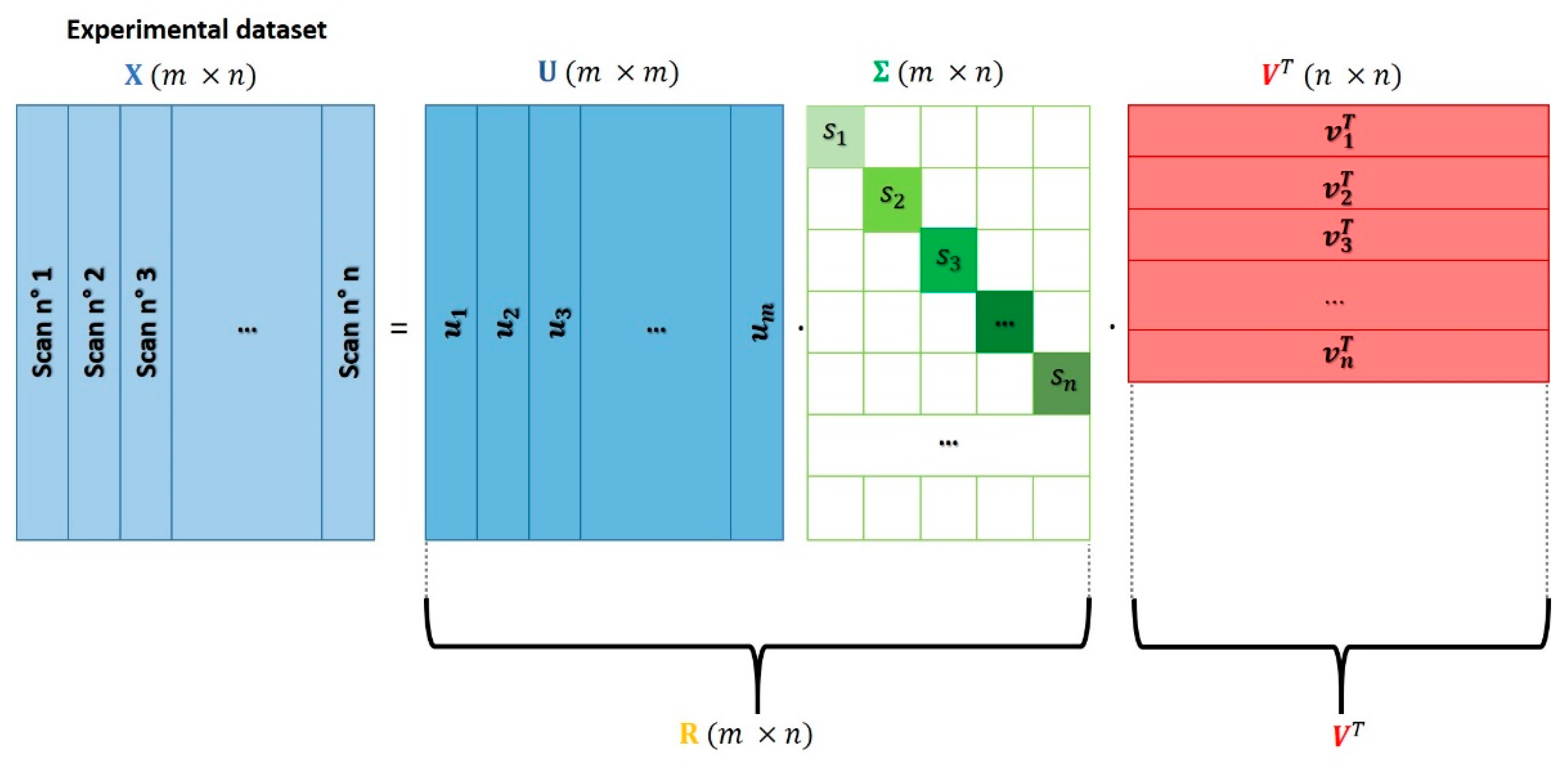
Generally speaking, PCA belongs to the family of unsupervised machine learning processing algorithms [21] and can be used in the analysis of a XAS dataset to correctly identify its rank. The PCA approach assumes that the XAS data mixture can be expressed as a linear combination of a fixed number of components weighted by their own fractions. The set of components employed in the spectral decomposition procedure must be independent to each other; moreover, they must be able to account for the highest variance of the XAS dataset including the noise. While different techniques can be applied in order to decompose a set of spectroscopic data on the basis of its principal components, a standard matrix factorization technique called singular value decomposition (SVD) is generally applied due to the fact of its robustness and accuracy. The SVD approach foresees the decomposition of the XAS data matrix in the product of three matrices:
where and are two square unitary matricse ( and ) while is a diagonal rectangular matrix ().
Figure 2 shows schematically the output of the SVD procedure. It is worth noting that this kind of decomposition is not unique and that there are different ways to perform it; in some of them, matrices or can be rectangular while squared. More information about the different algorithms employed to realize the SVD can be found in Reference [44].
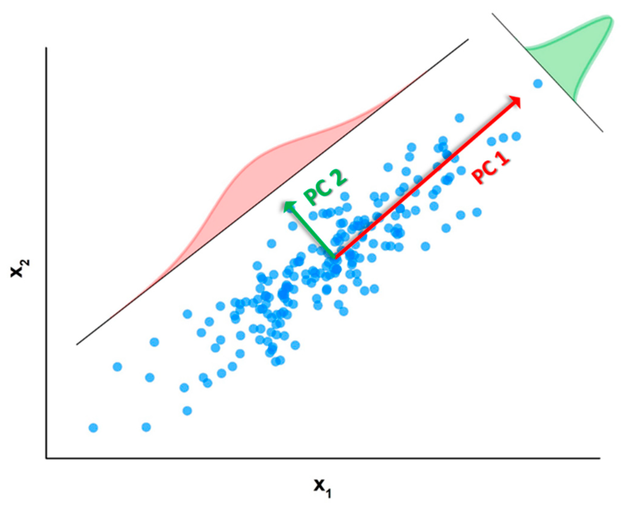
Matrix contains on its columns the eigenvectors of the covariance matrix associated to , i.e., which are the so-called principal directions or components. On the other hand, matrix shows on its rows the eigenvectors of the transpose of which, from a geometrical point of view, can be interpreted as the projection of dataset over the entire set of principal directions contained in . These vectors can be also interpreted as the principal directions (or components) taken directly from the rows of rather than from its columns. For the sake of clarity, in this work we will refer always to the name of principal components (PCs) as the columns of matrix . As a didactic representation, the principal components associated to a bi-dimensional dataset composed of 200 points are reported in Figure 3.
Finally, the diagonal elements of are named as singular values, and their magnitudes are connected to eigenvalues of the covariance matrix of through the following formula:
where and are the ith singular value and eigenvalue corresponding to and to the data covariance matrix, respectively. As already pointed out by Calvin in Reference [45], in the field of XAS analysis, the terms are usually referred to as the variances associated to the dataset principal components. However, this statement is true only if the XAS data are centred (i.e., the mean calculated over all the columns of has been subtracted to every spectrum composing ). Because in the XAS analysis, the dataset is usually not centred, the quantities retrieved by Equation (4) cannot be properly interpreted as the true data variances, despite the fact that they follow the same decreasing trend as a function of the component number (see Section 2.1.1). Nevertheless, the term variance is almost universally used in this context, even though the data mean centring condition is not satisfied [45].
The factors appearing in Equation (3) can be grouped as follows:
where . The columns of will correspond to the ones of scaled by the correspondent singular values; the connection of this expression with Equation (2) will be discussed in more detail in Section 2.2.
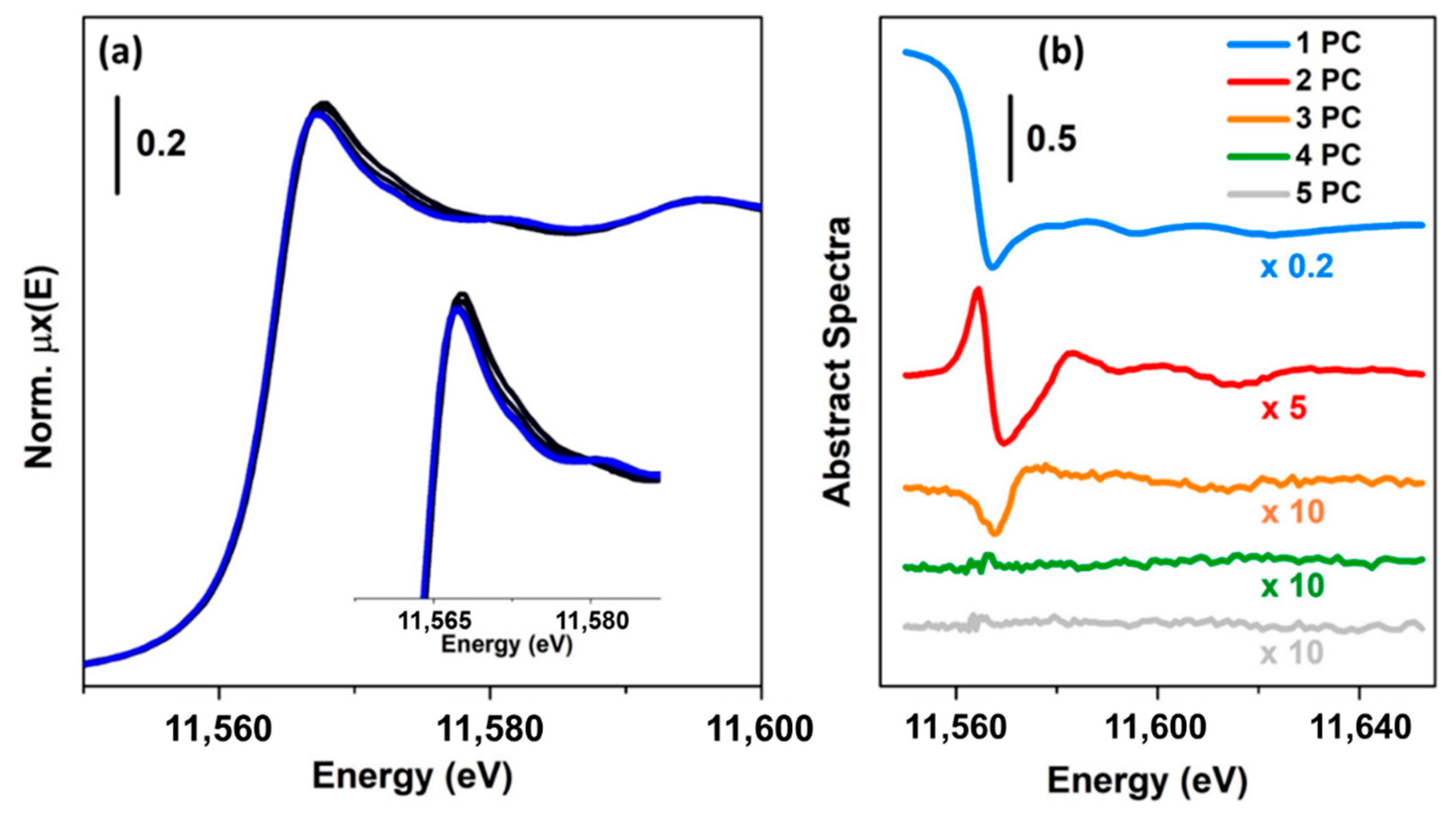
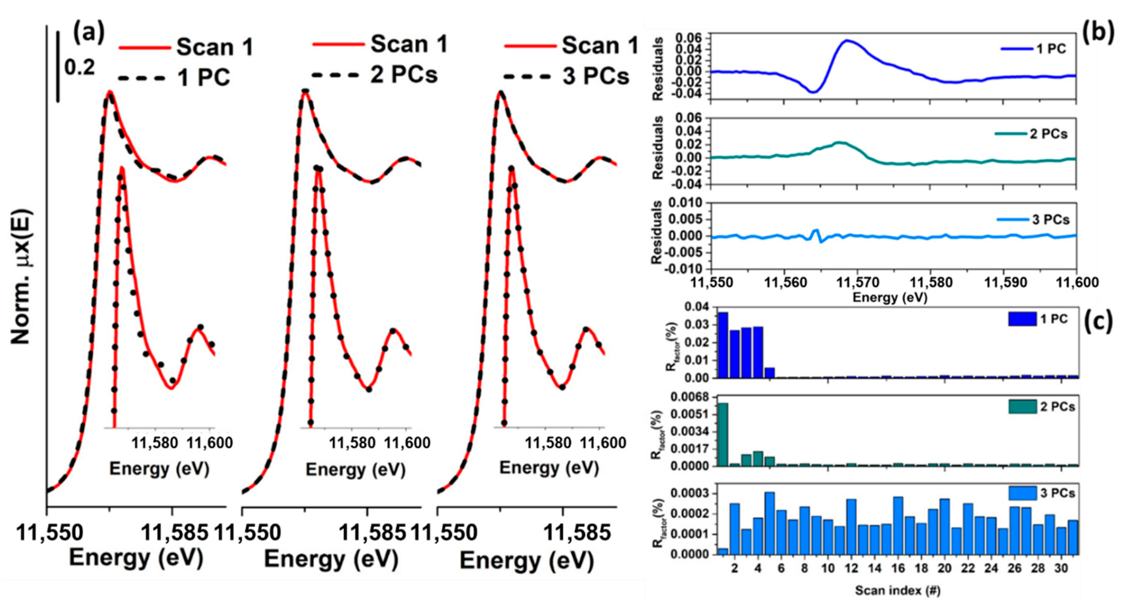
As an example, Figure 4 reports a XANES dataset, in part (a), and the related first five columns of (abstract spectra) in part (b), plotted in the same energy range. Because the first component is characterised by the highest variance, its contribution appears higher than the other components. In particular, it is interesting to note that its shape resembles an inverted XAS spectrum. The reason for the inversion depends on the output provided by the SVD decomposition (in some cases, it can be positive), while the similarity can be explained by the fact that was not centred. Because the first principal component needs to explain the highest variance of the dataset, it will assume a form resembling the mean of all the spectra composing the dataset. The second principal component captures the second highest spectral features of the XAS dataset, while the third one appears to be connected to minor but not negligible variations of the spectra. Starting from the fourth component, it is possible to see that they appear featureless on the scale of the XANES spectra. In particular, the distribution of their values, as a function of the energy, appears to follow a trend typical of the instrumental noise [45]. A second validation of this result can be obtained trying to analyse the residuals and plotting the %Rfactor related to the reconstruction of each spectrum of the XAS dataset as a function of the number of principal components involved, see Figure 5a–c. The %Rfactor is defined as: , where the subscript k denotes the number of principal components considered to reconstruct matrix , while the symbol is the Frobenius norm. If the XAS dataset is not properly represented by the chosen number of PCs, it will show, for certain scans, a higher indicating that one (or more) additional components are required to describe them. Once that the correct number of PCs is found, the values associated to the reconstruction of each spectrum must have comparable magnitudes as shown in Figure 5c.
On the basis of the results shown in Figure 4 and Figure 5, it is possible to conclude that the XAS dataset of Figure 4a can be properly described using only three principal components. Because each PC is independent to each other (i.e., they are orthogonal) their number represents a proper estimation of the rank of the XAS data matrix, corresponding to the number of chemical species associated to it. While the methods described above constitute a first qualitative approach to the analysis, different techniques have been developed in the field of the PCA in order to establish quantitatively the correct rank of a dataset. Among them, in the field of XAS, the scree test, the imbedded error (IE), the Malinowsky indicator factor (IND) and the Fisher test (F-test) are widely applied and will be discussed in more detail in the following section.
2.1.1. Quantitative Methods to Extract the Correct Number of PCs
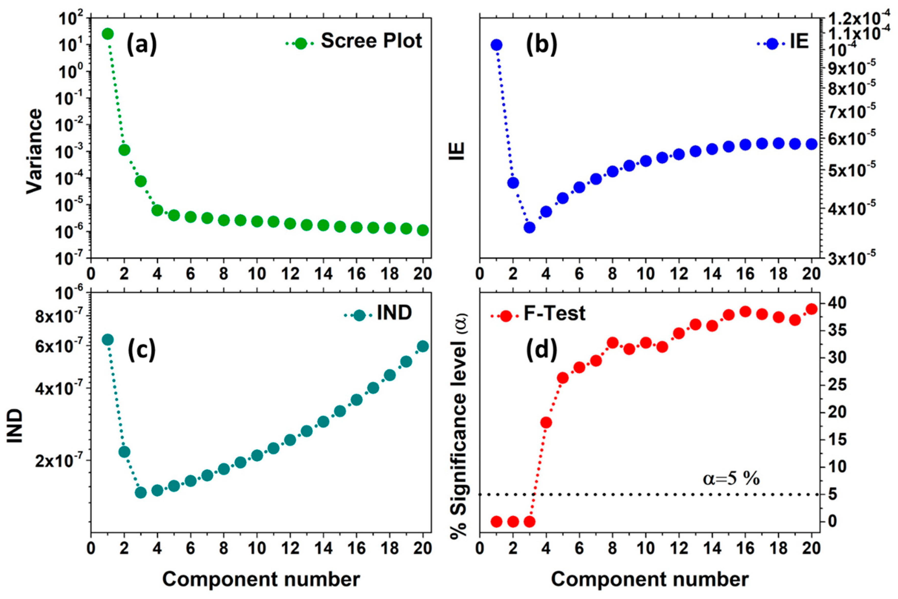
The first widely used approach is the scree test (or scree plot), and it consists in plotting the variance or the singular values magnitudes associated to each principal component versus their number, as shown in Figure 6a. As it is possible to see, after the first component, the variance associated to the components rapidly drops down, up to an elbow indicating the border between components having a real physical/chemical meaning (i.e., the number of species characterising the dataset) from those related to the data noise. It is worth noting, in fact, that the components associated to the noise must contribute approximatively in the same way to the dataset variation and for this reason they usually lie on a flat line.
The IE function is given by the following expression:
where k represents the number of components used to reproduce the dataset . If the experimental errors are distributed randomly and uniformly along each spectrum of , then the sum of the squares of the projections of the residuals, defined as: onto the noise-related PCs, should be approximately the same [47]. This means that the PCs representing the experimental noise must have approximately the same variances: . Hence, for k > N, Equation (6) can be rewritten as:
It follows that increasing the number of components, for k < N, the IE function progressively decreases until k = N, where it reaches a minimum corresponding to the proper number of PCs to consider. Then, for k > N, the IE assumes a slowly growing trend, as shown in Figure 6b.
Malinowski discovered an empirical function called IND function [47] which seems to be more sensitive than the IE function in its ability to pick-up the proper number of components [48]. The IND function is defined as:
Similarly to the IE functions, the IND estimator is calculated incrementally by increasing the number of PCs and, by definition, it reaches a minimum when the correct number of components is employed (see Figure 6c). However, it has been observed that, in this function, the minimum is more pronounced and can appear in situations where the IE does not exhibit any valley. More details about the IE and IND estimators can be found in References [47,48,49].
The Malinowski F-Test, reported in Figure 6d [47,48], is the last statistical method applied to determine the true dimensionality of a dataset. It is based on the observation that the reduced eigenvalues are constant for non-significant PCs [50]:
Because the values are still proportional to a variance, a Fisher test can be applied. The test starts from the smallest term, clearly associated to the noise, and proceeds to those values, with higher magnitude, until the first significant one is found. The kth component is considered significant on the basis of the Fisher test applied on its related standardized F-variable:
If the percentage of significance level (%SL), associated with kth F variable, is lower than a pre-fixed value (usually fixed to 5%), then the kth extracted component is accepted as a pure component.
Although these estimators have been applied with success in several XAS studies [1,14,25,51], it is worth noting that the identification of the number of PCs connected with the existence of determined chemical species critically depends on the amount of noise affecting the data, as shown by Manceau et al. [50]. In fact, deviation from the correct number of chemical species notably occurs when the level of the experimental noise is close to the variation of the data. Another cause of uncertainty in the estimation of the correct number of PCs must be found in an inconsistent normalization of the XAS dataset under analysis [50]. Moreover, if the concentration of some components is approximatively constant, or if the ratios of the concentration of some components are the same in the whole dataset, their independent contributions cannot be properly separated [37,50,52].
Finally, it is important to clarify the question regarding how many spectra are required for a proper identification of the significant components contributing to a XAS dataset. Because PCA is a statistical approach, one could think that, if the number of XAS spectra constituting a dataset is higher, there would also be a higher possibility to successfully identify all the contributing chemical species. That is ultimately not true, since PCA is a technique able to catch the highest independent variations of a dataset. It follows that it is preferable to have a lower amount of XAS spectra homogeneously sampling a chemical/physical process throughout its whole development, than a larger number of XAS spectra collected uniquely in determined moment of the reaction. Examples where the application of the PCA on a limited set of XAS spectra has been able to provide interpretable result can be found in the works by Beauchemin et al. [53], Lengke et al. [54] and Bugaev et al. [55], where the analysed XAS datasets were composed by six, eight and ten spectra, respectively.
2.2. Models Used to Decompose a XAS Dataset
As shown in Section 2.1, PCA appears to be a fundamental tool to correctly understand the number of pure species characterising a XAS dataset. Moreover, the PCA approach allows to decompose the set of data in a form resembling Equation (2): if the PCA of a XAS dataset leads to the identification of N PCs, Equation (5) can be rewritten as:
where the subscript N indicates that only the first N column of and have been considered in the reconstruction of . If the number of PCs has been chosen correctly, each residual spectrum of must resemble the white noise. It is interesting to note that among the various methods that can be adopted to decompose matrix as Equation (2), the one showed in Equation (11) is able to guarantee the highest approximation of (i.e., the lowest residual matrix), as stated by the Eckhart-Young theorem [56].
If analysed, matrices and possess the same dimensionalities of and , respectively. However, their set of spectra and concentration profiles do not have any spectroscopic meaning, as showed by Figure 4b. For this reason and can be considered only as a mathematical solution of Equation (2) and are usually named as the abstract set of spectra and concentrations of a dataset : and . Despite this problem, it is worth noting that the columns of can be combined together linearly in order to construct one or more pure spectral profiles with a chemical/physical meaning. This procedure is at the basis of some approaches quite used in the field of XAS data analysis. These include the target transformation analysis (TTA), the iterative target transform factor analysis (ITTFA) and the transformation matrix (TM) method. On the other hand, several methods been developed to realize Equation (2) without making any kind of transformations on matrix and , employing only some standard spectra or a set of selected spectral profiles for a single or multiple least-squares refinement. The most widely used are the linear combination analysis (LCA) and the alternating least squares (ALS) approaches.
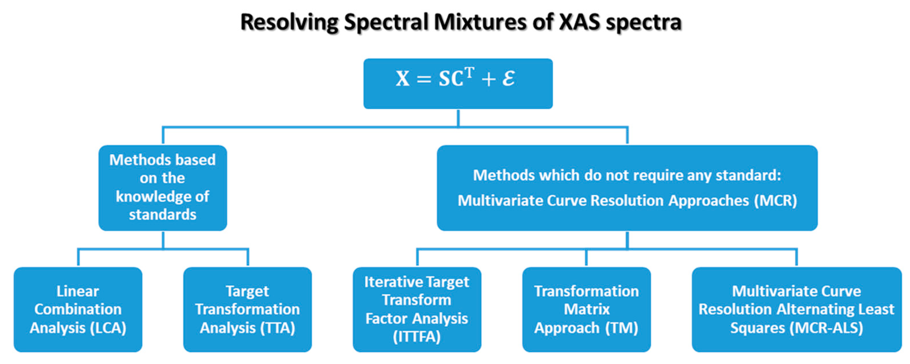
As schematically illustrated in Figure 7, all the methods cited before can be formally grouped in two classes: the methods requiring a priori knowledge of standard spectra (TTA and LCA) and the ones which allow blind source separation of the dataset (ITTFA, TM and ALS) which can be grouped inside the family of the multivariate curve resolution (MCR) algorithms. In the following, each cited method will be described in detail.
2.2.1. Methods Based on the Knowledge of Standards
Linear Combination Analysis
Given an experimental spectrum, if a set of k known reference spectra, named as standards, is supposed to correspond to the independent species present in the sample, they can be employed in Equation (1) to retrieve the related fractions through the following minimization procedure:
where is the ith standard spectrum involved in the reconstruction. This method is the so-called linear combination analysis (LCA), and it can be properly applied in the absence of non-linear effects, due to the sample thickness or fluorescence self-absorption, distorting the experimental data [3]. Equation (12) can undergo towards further modifications if one wants to optimize, besides the fraction estimations, secondary parameters such as the shifts in energy of each reference. It is possible, in fact, to construct, in this case, a function returning each selected reference, interpolated over a fine energy grid, depending on as: . These quantities, together with each term can then be refined minimizing Equation (12) through a non-linear least squares approach [57,58].
The LCA method can be clearly extended to the study of a dataset once that the number of components has been defined by means of PCA. However, it is worth noting that the LCA of a series of XAS spectra can be performed properly only under the hypothesis that the selected set of standards is able to describe adequately each spectrum in the dataset. Moreover, how it was described by Giorgetti et al. [59], it is required to safely exclude secondary processes affecting the measure, such as the loss or the dissolution of some part of the sample, which can make the mass-balance condition constraint incorrect. These phenomena can be detected by analysing the XAS background of each spectrum; if it appears globally stable, it is possible to conclude that the modifications of the XAS features are only due to the relevant physico-chemical processes and not to experimental artefacts. On these bases, the minimization procedure reported in Equation (12) can be realized employing each spectrum composing , resulting in a set of concentrations profiles which describe, for each scan, the amount of each reference characterising the experimental spectra composing the XAS dataset.
Target Transformation Analysis (TTA)
As stated before, PCA is able to provide the main N independent sources of variation of a XAS dataset but the retrieved abstract spectra and concentration values do not have any kind of physical/chemical meaning. Herein, it is possible to apply the target transformation approach in order to verify if some standard known spectra, usually named as target spectra, can potentially explain the variation of the spectral features of the XAS dataset [47,53]. The target transformation is a powerful method that allows testing a putative target without a priori knowledge or assumptions about the species present in the spectral mixture [53]. Basically, it consists in constructing the test spectrum as the linear combination of the abstract spectral profiles , by identifying the weights associated to the abstract spectral profiles using a least squares approach. This is equivalent to transform the known target spectrum in the reconstructed one using an oblique transformation:
The putative vector is accepted as a solution of Equation (2), if its spectral signatures can be reproduced based on the abstract spectra retained at the PCA step. A widely applied criterion used to establish if a XAS standard is an acceptable target is the SPOIL factor introduced by Malinowski, whose derivation can be found in References [47,60]. The idea is the following: if the target belongs to the dataset, it should be reproduced by the components as well as the original spectra; if not, it should add error to the data mixture spoiling it [45]. Malinowski classified the SPOIL values using three thresholds: a target spectrum can be considered acceptable if the related SPOIL value is lower than three, moderately acceptable if the value is within three and six, and unacceptable is it is higher than six [53]. When all the N standard spectra have been identified and tested to be acceptable using the SPOIL test, their transformation matrix , containing on its columns the least squares weights appearing in Equation (13) can be inverted and multiplied to in order to retrieve the related set of pure and meaningful concentration profiles, i.e., and . Furthermore, if required, the elements of can be renormalized by their sum, so that the sum on the elements of each row of is be equal to one. However, this implies that their projection over and is not complete causing a small increase of the residuals, i.e., . In general, this is an effect that appear every time that a solution, coming from the application of a transformation matrix on the abstract spectral and concentration profiles, is modified in order to provide a feasible set of spectra and concentrations values. Nonetheless, the differences among and are quite small and usually it is possible to assume . The same statement can be asserted for the ITTFA and MCR-ALS approaches (see Section 2.2.2).
The main problem of the LCA and TTA approaches is that they require a priori knowledge of XAS standards involved in the description of each single spectrum composing a dataset. There are, in fact, several cases where it is not possible to know a priori which are the species characterising a set of measurements. At the same time, some reference spectra corresponding to determinate compounds are unavailable because simply unknown or difficult, if not impossible, to obtain synthetically. In order to overcome this problem, several methods belonging to the MCR family have been applied and developed as it will be discussed in more details in the following sections.
2.2.2. Multivariate Curve Resolution (MCR) Approaches Applied to XAS Data
Multivariate curve resolution (MCR) is a generic denomination for a family of approaches aimed to realize the decomposition in Equation (2) from the sole information derived from the original data matrix, including the contributions coming from different chemical species [61]. Among the large number of methods which have been developed for this purpose [61], in the following sub-sections three main approaches are listed and described which allow retrieval of relevant results in the analysis of XAS datasets. These include: the iterative target transform factor analysis (ITTFA), the transformation matrix approach (TM) and, finally, the alternating least squares method (ALS). Among them, only the ITTFA and the ALS approaches can be employed to realize the so-called blind source separation of the dataset components [21], especially for the XAS datasets showing large variations of their spectral features. On the other hand, the TM method is mostly suitable for those datasets composed of spectra presenting limited variations in the XAS spectral features. However, the resulting set of spectra and concentrations require a careful a posteriori assessment by the user, who needs to discriminate the feasible solutions retrieved from Equation (2) based on their physico-chemical and spectroscopic reliability. Generally speaking, although a priori knowledge is not mandatory in implementing such approaches, the availability of complementary information on the investigated systems and chemical processes often plays a crucial role in retrieving a meaningful solution.
In case of the MCR approaches, some rules of thumb should be followed to have higher possibilities to retrieve a feasible solution from Equation (2). As in the PCA case, it appears more useful to have a lower amount of XAS spectra but homogeneously sampling the entire reaction process rather than a larger dataset contained several spectra acquired only in some specific moment of the experiment. The reason for this choice stands in the possibility to obtain a uniform distribution of the variations of the XAS spectral features during the entire measurement, thus increasing the probability to avoid a deficiency in the estimation of the rank of the dataset. Moreover, this methodology helps in identifying an initial set of spectra and concentration profiles as close as possible to the ideal, pure ones, leading the subsequent refinement towards a chemical/physical interpretable solution. Finally, it is worth to mention here a fundamental result by Manne [62], who proposed two theorems aimed at defining when a dataset can be uniquely and correctly resolved. These states that: (i) the concentration profile of a determined compound can be correctly resolved if all the components inside the range of scans, where it is supposed to appear and evolve (i.e., its concentration window) are also present outside; (ii) the pure spectrum of a compound can be correctly recovered if its related concentration window is not fully embedded into the window of another component [61]. If these requirements are satisfied, a feasible solution can be identified using an MCR approach.
Iterative Target Transform Factor Analysis (ITTFA)
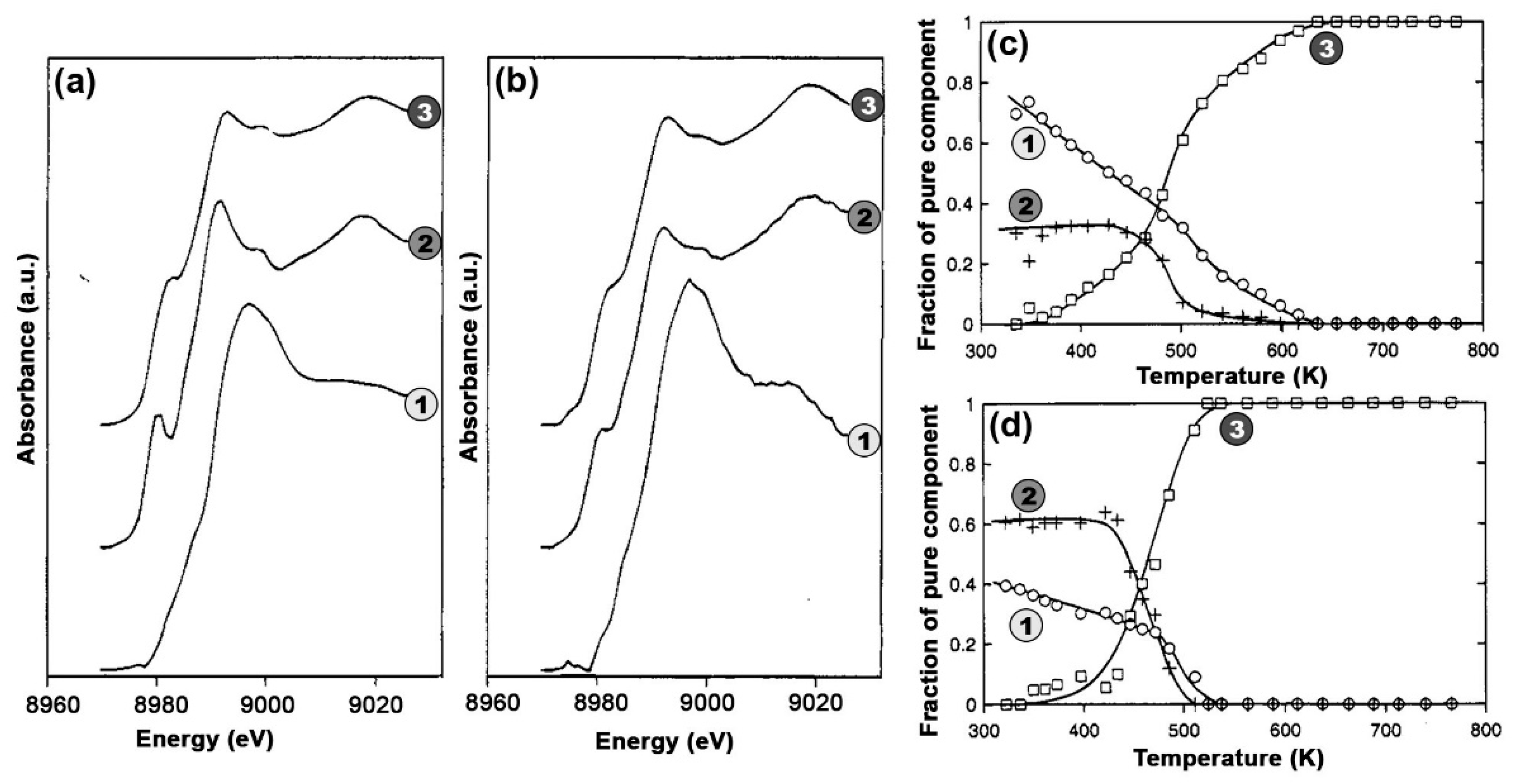
The first application of an MCR approach to a set of XAS data has been realized by Fernandez-Garcia et al. [14]; see Section 3.2.1 for additional information. The authors were able to correctly estimate three pure Cu K-edge XANES spectra characterising a series of measurements involving two bimetallic CuPd/zeolite samples during a temperature-programmed reduction (TPR) experiment employing a self-modelling curve resolution algorithm referred to as ITTFA [47], currently implemented, e.g., in the XAS code PrestoPronto [63]. The first step of this method consists of the application of PCA on the acquired measurements in order to identify the number of pure species characterising a dataset and its related abstract spectral and concentration profiles: and . Since the selected components do not have any spectroscopic meaning, they need to undergo towards a series of transformations regarding their rotation in the component space. Herein, the abstract concentration profiles are first subjected to an orthogonal rotation called varimax [47], allowing to align each column of along the pure unknown concentration profiles , and revealing the scan number corresponding to the spectra where the maximum concentration of each pure component is observed. Furthermore, a test concentration matrix is generated considering for each component a delta function (), with an amplitude equal to one, peaking in correspondence of the temperature value where the maximum intensity of the related varimax-rotated concentration profile is detected. The transpose of identified test matrix can be multiplied by giving rise to the following transformation matrix:
Afterwards, the matrix is used to convert in as:
The recovered spectral profiles of can be seen, algebraically, as the projection of the matrix columns over the vector base defined by . Clearly, the direct solution provided by Equation (15) can be, sometimes, not chemically/physically correct. It is possible, in fact, that one or more concentration profiles could have some negative values. This problem can be easily solved forcing the negative terms to be equal to zero; at the same time the concentration values referring to each scan can be scaled by their sum imposing, in this way, the mass balance condition. Afterwards, the constrained version of is set as the appearing in Equation (14), then the entire procedure described above is repeated until the Frobenius norm between two corrected concentration matrixes coming from two consecutive iterations is lower than a user-defined value. An alternative criterion foresees to simply stop the refinement when a maximum number of iterations is reached [64]. Finally, the transformation matrix, associated with the last refined form of matrix , is used to recover the matrix containing the pure spectral profiles as . If some spectrum of matrix has negative values, these can be set directly to be zero, making the solution spectroscopically interpretable.
While the ITTFA appears to be an intriguing approach, because it does not require any standard or a priori knowledge of the system under study, it also presents some limitations. Starting from the initial set of concentration profiles, the algorithm provides a very quick improvement towards the correct profile, but afterwards the process dramatically slows down and it reaches with difficulty the required set of pure profiles [64]. A second relevant problem connected with this approach is the rotational ambiguity phenomenon which affects almost all the algorithms attempting to realize the blind source decomposition of matrix and will be discussed in mode details in the following.
Transformation Matrix Approach (TM)
The transformation matrix (TM) approach was introduced by Smolentsev et al. [1], and it is currently implemented in the PyFitIt software for the quantitative analysis of XANES spectra [65]. This method is similar to the TTA, and it is based on the observation that the decomposition shown in Equation (11) is not unique. In fact, it can be rewritten as:
where is a is a square invertible matrix, called transformation matrix. Because the matrix product is equal to the identity matrix , the variation of each element of does not have any kind of impact on the decomposition shown by Equation (11). However, the abstract spectra and concentration profiles can be grouped in the following way: and . Afterwards, the elements of can be properly moved in order to retrieve a set of pure spectra and concentration profiles spectroscopically interpretable and representing a solution to Equation (2). From a practical point of view, this step is realized in PyFitIt through the usage of a set of sliders which can be directly moved by the user. Because matrix is a squared matrix with dimensions , the general number of sliders that could be moved would be equal to . While for the simplest case (i.e., ) four sliders can still be moved without large difficulties; however, when the number of species in the dataset starts to increase, this approach appears to be not so practical. Nevertheless, the possibility to impose a set of physical constraints can substantially reduce the number of sliders to move, together with their range of variation. As already stated in previous sections, it is possible to include the non-negativity of the spectral and concentration profiles and the mass balance condition. While the first two constraints can be implemented looking for a set of parameters of able to provide absorption coefficients and concentration values that are non-negative, the mass balance condition is less straightforward to realize. In general, one should move the sliders in order to guarantee for each scan that the sum of all the concentration values is equal to one. If the XANES profiles, composing the dataset, only show small variations in their spectral shapes and intensities, it is possible to impose the normalization of the spectral profiles through the following formula:
where is the normalization factor used to scale the ith spectrum determining , while Emin and Emax are the minimum and maximum energy values of the XANES range, respectively. If the absorption edge region does not undergo towards abrupt changes, the normalization factors remain almost unvaried from spectrum to spectrum: (based on our experience, the variations of involve usually the third decimal digit), allowing to maintain the same jump of absorption normalization (i.e., , where is the energy edge position) approximatively constant for each XANES in the dataset. The requirement of the dataset normalization ensures the equality between each element of the first abstract concentration of Equation (17) (i.e., ) and the normalization coefficient related to the first abstract spectrum: , where while is the first vector columns (i.e., the first abstract spectrum) of matrix . This result can be used to guarantee the condition . In fact, it is possible to show that the normalization of the components reduces the number of matrix transformation elements from N2 to N2–N and determines the following simplification:
The presence of these constraints obviously limits the range of variation of the elements of and only the construction of a proper set of strongly selective constraints can lead to the isolation of a series of XANES components extremely close to the real physical/chemical solution. These can foresee, for example, the requirement that a particular spectrum in the dataset could be considered as pure. It follows that a selected column of could be recovered using a least squares approach as in Equation (13) in order to allow the equality between the pure spectrum and the experimental one. The number of sliders to move is then reduced to . Furthermore, other constraints can be clearly implemented and imposed in order to reduce the number of free sliders, as described in Reference [65]. As an example, Figure 8 reports the solution found by applying this approach to the set of Pt L3-edge XANES spectra shown in Figure 4a.
Applications of these methods can be found inSection 3.2.2 and Section 3.2.3.
The ALS approach, usually referred to as MCR-ALS, is a spectral un-mixing method introduced by Tauler and co-workers [66,67,68]. The MCR–ALS method has been largely used during the last two decades in different fields of research, ranging from chromatography to image analysis [61,68]. This method was applied for the first time in the field of XAS data analysis in the pioneering work by Conti et al. [25]. Afterward, an increasing number of research groups have begun to use it in the analysis of XAS datasets relevant to different research areas such as batteries [25], quantum-dots formation [24], solid-state chemistry [22] and heterogeneous catalysis [15,33,34,35,51]. The main reasons behind the spread of this algorithm can be found in its simple implementation and robustness of the code as well as in the availability of practical graphical user interfaces (GUIs) and packages which facilitate its application [69,70].
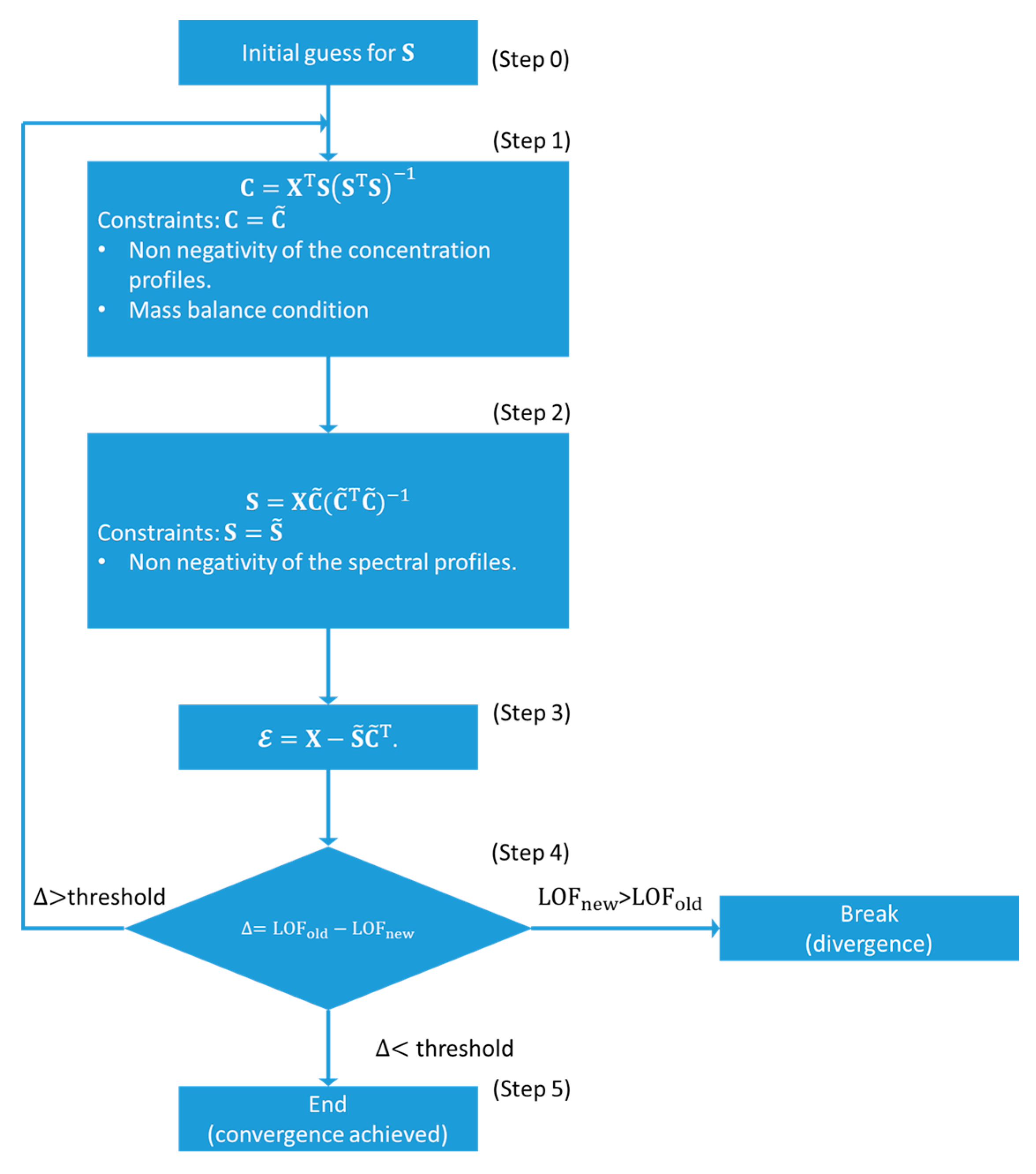
The flow diagram at the base of the MCR-ALS algorithm is shown in Figure 9. In contrast to the approaches presented before in this Section, this method is not based on the rotations of the abstract spectral and concentration matrices. The first step of the algorithm consists in the estimation of a set of spectra or concentration profiles, the number of which should correspond to the number of signal-related PCs. This step can be realized using different methods. For the analysis of XAS data the most widely used are the evolving factor analysis (EFA) and the simple-to-use interactive self-modelling mixture analysis (SIMPLISMA) algorithms [71,72].
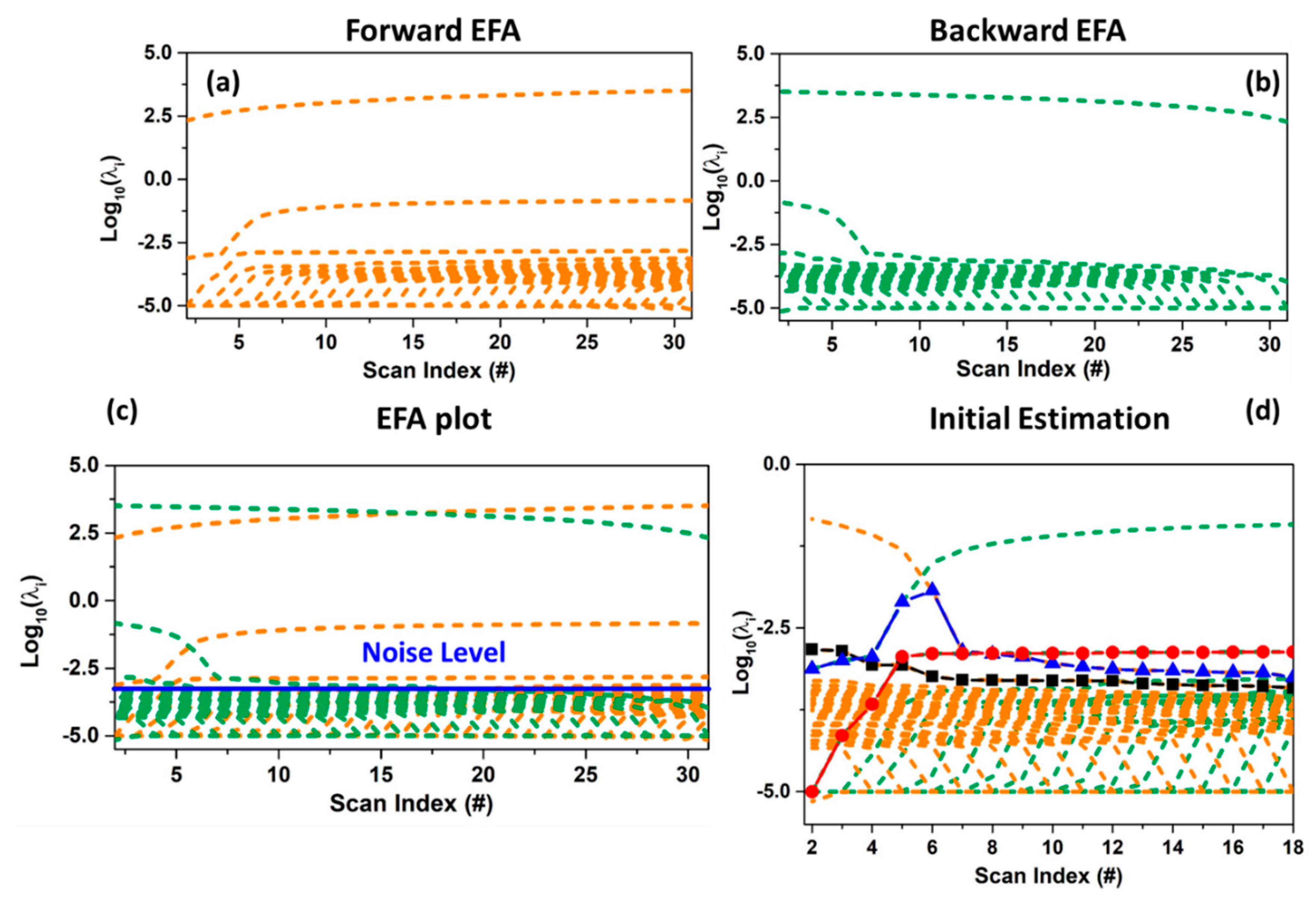
The EFA algorithm monitors the changes in the significant number of components (not noise related) during the progress of the measurement by performing many local rank analyses of sub-datasets with increasing size, obtained including every time a new spectrum. This step is realized from the first scan (forward EFA, see Figure 10a) till to the last one and vice versa (backward EFA, see Figure 10b) [25,61,73]. Evolving factor analysis results in a plot showing the log-scale of the eigenvalues of the covariance matrix of each sub-dataset of varying during the evolution of a physical or chemical variable (e.g., time or temperature). When the complete dataset is considered at one extreme of the plot (forward or backward), the number of eigenvalues curves above a user-fixed threshold (indicating the noise level) defines the total rank of the data mixture (i.e., the number of chemical species characterising it) (see Figure 10c). On the basis of this plot, supposing the existence of N pure components, the concentration profile of the first contribution is obtained combining the 1st significant eigenvalues line of the forward EFA plot with the Nth line of the backward EFA plot; the profile of the second contribution relates the line of the 2nd eigenvalues curve in the forward EFA plot to the (N−1)th line of the backward EFA plot, and so forth. In general, each element of a determined concentration profile is selected as the smallest value between the forward and backward combined eigenvalues lines (see Figure 10d). Furthermore, the retrieved concentration values can be rescaled, for each scan, for their sum, maintaining the validity of the mass balance condition, and then employed in the ALS refinement.
On the other side, the mathematical principle of the SIMPLISMA algorithm consists in the identification of a set of spectral or concentration profiles, equals to the number of the significant components. Each of them must experience a non-zero contribution from one and only one mixture component [61,74]. The identification of these spectral profiles is realised by the generation and the analysis of a series of vectors containing as elements a set of statistical variables expressing the level of purity associated to each spectrum in the dataset. The vector proper of the first pure specie is retrieved just as the ratio among the standard deviation and the mean of the XAS dataset calculated over its rows: . Herein, will have a number of elements equal to the number of scans comprising . The choice of defying this vector through is connected to the evidence that the standard deviation is generally higher for those scans where the concentration values of one component is significantly larger than the intensities of the others present in the chemical mixture. On the other hand, reflects the intensities of the concentration profiles of the individual pure components and, for this reason, it is used to scale the quantity [61]. Furthermore, the equation defining is corrected in order to account for the noise effects which can lead to a wrong identification of the purest spectra in the dataset, by adding a fixed value to the denominator of , usually taken as the 1–5% of the maximum value of . Under this correction, the vector assumes the following form: . The position, in , of the element with the highest intensity is able to provide the scan index of the first purest spectrum present in the XAS dataset. The vectors associated to the subsequent pure spectral profiles (the second, the third, etc.) must be independent (i.e., orthogonal) to each other. This requirement is realised through the calculation of a set of weights (with i = 2, 3, …) which will be then applied progressively to the ratio . These quantities are retrieved directly from the covariance matrix of . A detailed description of how these weights are constructed mathematically can be found in chapter 3 of Reference [61]. Finally, as already described for the vector, the position of the maximum value of each new weighted vector provides the scan number corresponding to the ith purest XAS spectrum. In case one wants to retrieve the purest set of concentration profiles, the same procedure described above needs to be repeated with the exception that the mean and the standard deviation of the dataset are extracted over the columns of .
Clearly, if the dataset does not exhibit any pure spectral profile, the algorithm will identify the most different spectra or concentration values among the experimental ones. It follows that, usually, the output profiles provided by this method cannot be associated to determined pure components and their further refinement through an ALS approach is strongly advised.
Supposing that the MCR-ALS initialization has been realized using a set of spectra , the related concentration matrix can be obtained, using a least squares approach, minimizing the square of residuals between the experimental XAS dataset and the approximated one: which lead to the linear least squares solution: (step 1). Afterwards, a set of constraints must be imposed on to guarantee physico-chemical meaningfulness of the retrieved concentration profiles. As described in the precedent sections, dealing with XAS spectra it is possible to apply only two kind of constraints: the non-negativity of the spectra and concentration values and the mass balance condition (only if there are not phenomena involving the lost or dissolution of the sample under measurement). It follows that the negative elements of each column of are set to zero while the row elements can be scaled by their related sum ensuring the condition , where is the element of matrix sited in row i and column (scan) . Afterwards, the corrected matrix is involved in the calculation of the new set of spectral profiles minimizing, for a second time, the squared residuals between and the reconstructed dataset: , the solution of which is: . The negative values of are then forced to be zero, converting in (step 2). It is worth noting that the alternating computation of matrices and in the linear least squares approach followed by setting negative values to zero and by imposing the concentrations closure is simple but very crude and can make the algorithm quite slows, especially if the XAS data matrix is composed by several spectra. This problem can be solved employing some non-negative least squares algorithms (implemented in the most widely used software for data analysis such as Python, MATLAB and Wolfram Mathematica) which provides, as solution, a positive set of spectra or concentration subjected to linear constraints criteria (i.e., the mass balance condition) [75].
The corrected version of and can be employed to generate as: (step 3). Finally, the residual matrix is used for the calculation of the so-called lack of fit parameter (LOF) (step 4):
After the calculation of the LOF parameter, using Equation (19), for the first iteration (i.e., LOF1), the ALS routine is re-started deriving a new set of concentration profiles from step 1 using the corrected spectral profiles obtained from step 2 of the first cycle. The procedure then continues as described before until the LOF parameter for the second cycle is calculated (LOF2). Once this step is completed, the difference within LOF1 and LOF2 is evaluated. If this quantity is lower than a user defined value or threshold (usually 0.1%) the convergence is achieved and the ALS routine is stopped, otherwise the spectral profiles are employed in step 1 of the third cycle and so on. It is possible that among two or more cycles the LOF parameter starts to increase, indicating the divergence of the routine; in this case the algorithm is automatically stopped.
As for the ITTFA approach, the main weakness of the MCR-ALS algorithm stands in this poor convergence and in the so-called rotational ambiguity. This phenomenon expresses the fact that there is not a unique solution for the task of decomposing the XAS matrix into the product of two positive matrices and [64]. In fact, as showed for the TM approach, it is always possible to decompose as: . This evidence indicates that sets of spectra and concentration profiles with different shapes can reproduce the original dataset with the same fit quality. It follows that the final result retrieved by the ITTFA and by the ALS approaches strongly depends on the initialisation of the routine, especially when the spectra composing the experimental dataset are similar to each other [61]. Different ways to assess the ambiguity of a solution can be found in References [76,77,78,79]. A common way to decrease or suppress this phenomenon foresees the usage of further constraints in the algorithm. These can involve, for example, the requirement that a pure spectrum or concentration profile could correspond to a determinate XAS standard or concentration values retrieved by other techniques (e.g., UV spectroscopy [32]). A second method requires that different datasets, supposed to be characterised by the same components, could be merged and analysed together in order to increase the probability to have a certain region of the data matrix where a particular species is dominant over the others. This procedure helps the initialization of the algorithms to identify, from the analysis of the dataset, a proper initial set of spectral and concentration profiles closer to the real solution. An example where this strategy provided good results can be found in Reference [51], where multiple XANES datasets collected on Cu-zeolites (chabazite) samples with different Si/Al and Cu/Al ratios, during thermal pre-treatment process carried out under consistent conditions, were joined in one larger dataset (see Section 3.1.1).
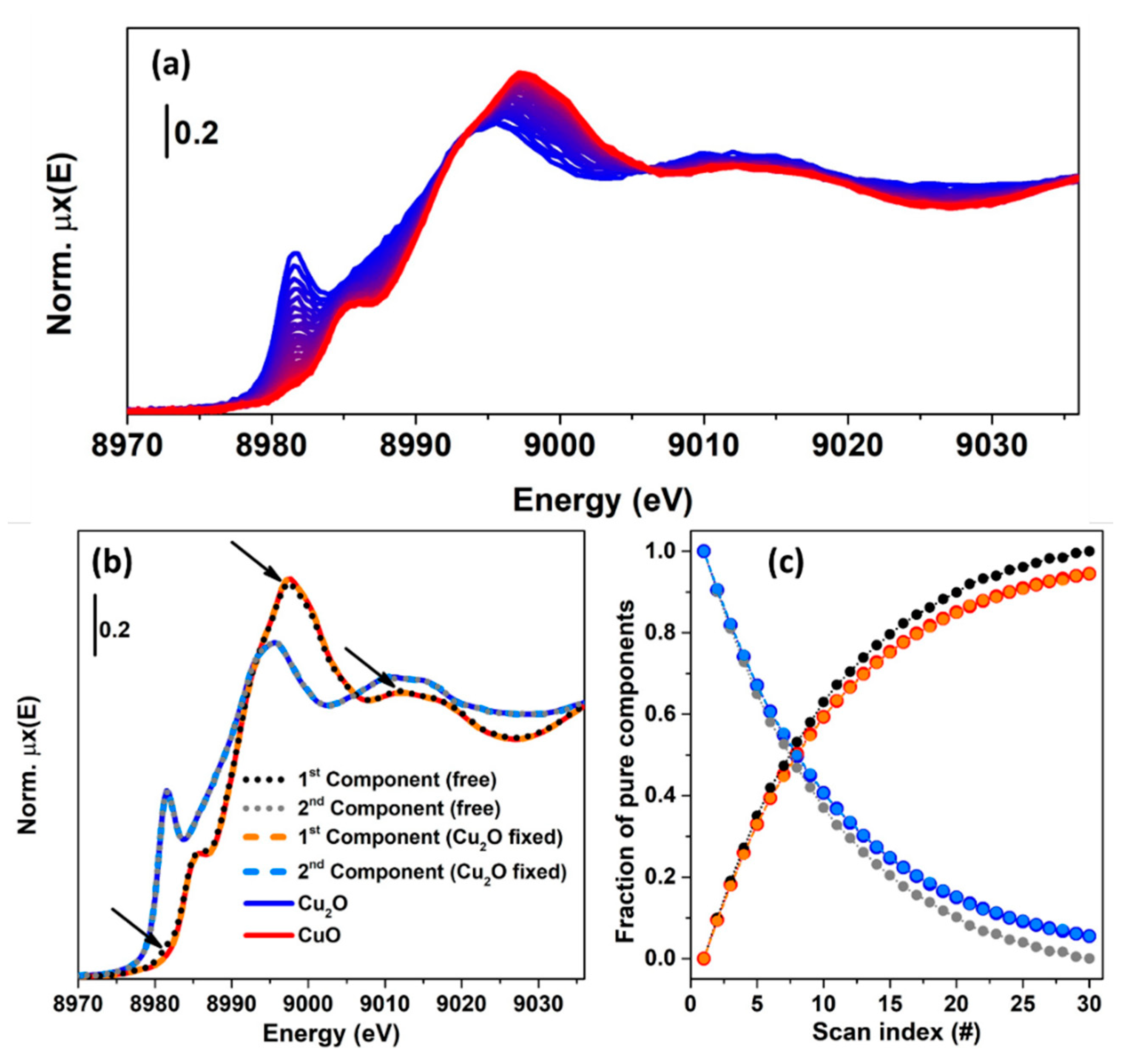
In order to clarify the concept of rotational ambiguity, two examples are reported in the following. In both of them, the same spectra corresponding to Cu K-edge XANES for CuO and Cu2O oxides have been considered. In the first case, a theoretical XAS dataset composed by 30 spectra, see Figure 11a, is generated on the basis of two concentration profiles following the kinetics curves: and , where denotes the scan number (or time). A noise matrix composed of 30 vectors, having their values selected following a normal distribution with mean 0 and standard deviation equal to 0.005, was added to the noise-free theoretical dataset in order to simulate the effect of the instrumental error in the measurement. The MCR-ALS routine, shown in Figure 9, was initialized using the EFA algorithm. Without any constraints, the algorithm converged after 21 iterations. The set of pure spectra and concentrations profiles are reported in Figure 11b,c (dotted black and grey curves). Focusing on the spectral profiles, small differences appear among the ALS retrieved spectra and the reference ones. These are localized around the rising-edge (approximately 8982 eV), the white line (approximately 8995 eV) and the post edge (approximately 9028 eV) features and refer exclusively to the first component, while the second is approximatively equal to the spectrum of Cu2O. On the other hand, bigger differences appear analysing the concentration profiles. It is possible to see, in fact, that the concentrations of the pure spectra retrieved without any constraint slightly deviated from the real values. As described before, the deviations involving the extracted spectra and concentrations were connected with the rotational ambiguity affecting the solution of Equation (2). Indeed, the ALS routine converged towards one of the several minima. The requirement that one pure spectrum corresponds perfectly to the Cu2O reference drives the algorithm to identify the correct solution (convergence after 19 iterations), as shown in Figure 11b,c, where the constrained pure spectral and concentration profiles (orange and azure dashed curves) coincided with the standards.
The example showed before demonstrated that under a proper set of constraints, the ALS algorithm can provide a solution approximatively equal to the real one. However, it worth noting that the possibility of reaching a meaningful result depends also on the initial estimation of the spectral or concentration profiles. In the case illustrated in Figure 11, the theoretical dataset was characterised by two species, which, at scan 0, had a relative fraction set to 1 (Cu2O):0 (CuO). This fact, as stated before, helps the EFA algorithm (and the SIMPLISMA algorithm as well) to identify a set of spectral profiles closer to the real ones.
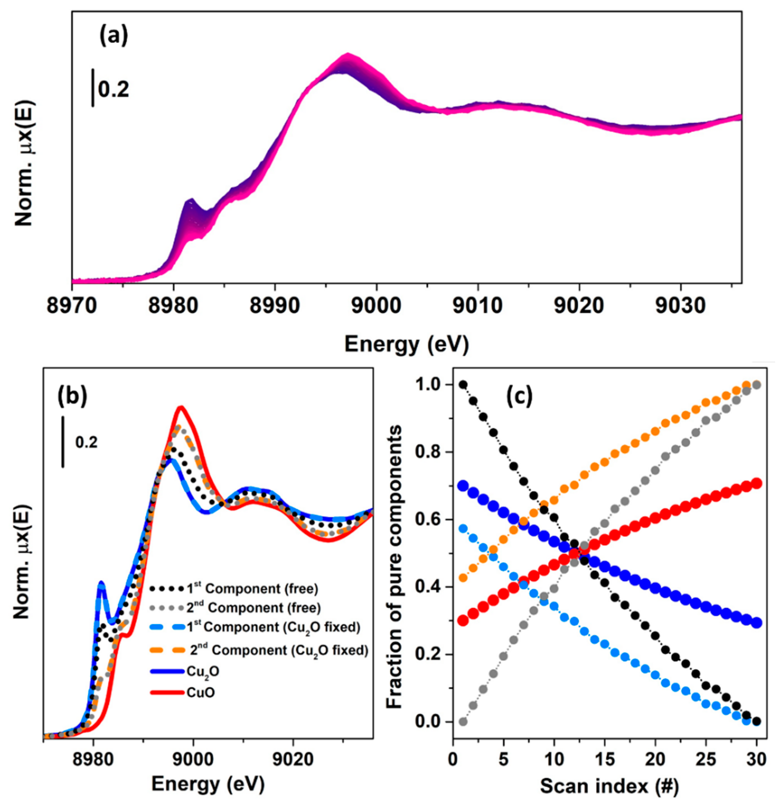
In the second case, see Figure 12a, a XANES dataset was generated by combining the reference spectra using two kinetics curves having the following equations: and . It is possible to see that during the thirty scans the relative fraction, for both the species, was never equal to one. Moreover, the magnitudes of the kinetic constant this time are lower than in the precedent case, indicating a slow variation of the simulated oxidation process. This fact has a strong influence of the result retrieved by the MCR-ALS analysis, as shown in Figure 12b,c. Herein, it is possible to observe that the solution provided by the unconstrained optimization (convergence after 22 iterations) led to a wrong set of spectral and concentration profiles, see the dotted, black and grey concentrations.
At the same time, the introduction of a stronger constraint (convergence after 13 iterations) in the routine, i.e., fixing the Cu2O reference spectrum, still does not lead the algorithm to solve correctly the problem. In this case, the first component and the spectrum corresponding to Cu2O are, as expected, identical. This implies that two among the four elements of the matrix causing the rotational ambiguity effect, are fixed. However, the remaining two elements are responsible of the wrong solution related to the second component (orange, dashed curve in Figure 12b) whose incorrect concentration values are compensated for by the introduction in the ALS-retrieved spectrum of CuO of spectral features proper of the Cu2O compound which is required to satisfy the mass balance condition. As told before, under circumstances equivalent to the one presented in Figure 12, only the introduction of further strongly selective constraints, such as the knowledge of a kinetic model, can orient the algorithm toward a spectroscopically meaningful minimum value [61].
Evaluation of the Level of Ambiguity Affecting a MCR Solution
As showed in the precedent examples, the rotational ambiguity phenomenon represents the main hurdle for all the described MCR approaches. It has been shown that the application of a hard set of constraints in the pure factorization problem shown by Equation (2) can lead to the identification of a solution that can often be considered extremely close or even coincident to the correct one. Whenever this is not possible, one might be interested in computing not only a single factorization of Equation (2) but the full range of all its solutions obeying a certain set of user defined constraints. Because all these sets of concentration and spectral profiles must be associated to a determined sequence of elements of the transformation matrix, it is possible to visualize the region of (where is the number of the elements of matrix generated considering PCs) named the area of feasible solutions (AFS). Furthermore, once these regions have been delimited, they can be employed to investigate the extent of unresolved remaining ambiguities [61].
In the field of chemometrics, several approaches have been developed in order to account for all the possible feasible solutions and to identify the bands of the maxima and minima variation of the spectral and concentration profiles solution of Equation (2). Assuming the existence of N chemical species, one of the most promising approaches consists of performing a change of coordinates and representing the columns and rows of the experimental data matrix in the U and space [74]: in the U space, the coordinates of the n data columns are while in the the m data rows assume the form of . Furthermore, it is possible to demonstrate that the normalisation, realized by dividing each new coordinate sited in U and by and , respectively, reduces by one unit the dimensions of the data representation. In the particular case of a two- and three-component system, these projections can be properly represented graphically in one- and two-dimensional plots together with the ensemble of feasible spectra and concentration profiles, which can be obtained exploiting determined computational geometric approaches or the grid search method [74,80,81]. This procedure facilitates the graphical representation of rotational ambiguities in all the MCR results and provides a good estimation of their impact on the retrieved solution of Equation (2). More details about this method can be found in Reference [61] as well as in the review provided in Reference [82].
In the field of XAS, to the best of our knowledge, the only two works where the AFS analysis is taken into account deals with the TM approach, foreseeing the multiple minimization of a penalty function , directly depending on the values of the spectral and concentration profiles [65,76] and expressed in the following form:
where , and are the elements of the vectors representing the spectral and concentration profiles retrieved from Equation (16) and depending linearly for the elements of matrix : and . is a Heaviside function that returns 0 if the spectral values are higher or equal to 0 or 1 for their negative values, while is a second function, associated to the concentrations profiles, that returns 0 for those concentrations within 0 and 1, while it is equal to 1 if this last condition is not satisfied. Several other constraints can be employed in order to reduce the AFS, such as the mass balance condition which, in the TM approach, can be simply realized exploiting Equation (18). By randomly initializing function and minimizing it for a considerable number of iterations (i.e., 1000 or more) it is possible to obtain a graphical representation of all the combinations of the elements of the transformation matrix satisfying the required constraints, determining, in this way the AFS of the XAS dataset.
2.3. Spectral Decomposition of a XAS Dataset: Differences among the XANES and EXAFS Region
So far, an overview on the principal methods used to decompose a XAS data matrix has been provided. It is worth noting that in the previous sections, the general term XAS has been used instead of the more specific ones: XANES and EXAFS. This choice is attributable to the fact that in the field of XAS data analysis, there are works applying these spectral decomposition methods in both regions. However, it is possible to verify that, at the moment, the number of articles connected with the analysis of the XANES region is higher than ones related to EXAFS. The reasons are multiple. First of all, it is worth noting that the XANES part of a XAS spectrum is usually collected faster than the EXAFS part; moreover, the spectral features affecting a XANES spectrum are always more distinguishable than in the EXAFS. The second reason is more conceptual, and it is still debated. Various works have been written dealing with the application of PCA and MCR approaches on EXAFS spectra [83,84]. However, considering the application of the PCA analysis on a set of EXAFS spectra, some ambiguities on the retrieved result can appear. As stated by Klementiev in Reference [85], the EXAFS region is described by a sum of modulated sine functions. These form a complete set of vectors and, for this reason, they can be linearly combined to reproduce any kind of function. Moreover, the functional shape of EXAFS makes each spectrum strongly correlated with any others, regardless of spatial structural correlations, possibly translating into ambiguities in the PCA solution. A clever solution to this problem is the one provided by Rochet et al. [35], and it consists in processing by PCA the entire XAS spectra as they are (XANES + EXAFS), exploiting the dominant fingerprints of the XANES part to drive the PCA algorithm to suggest a reasonable number of pure species characterising the dataset. This result is made also possible thanks to the usage of a Quick-EXAFS monochromator, offering unique capabilities for the sub-second time-resolved characterisation of catalysts under working conditions [86,87]. Afterwards the MCR approaches can be applied to decompose the XAS dataset and, once a feasible set of pure spectra and concentration has been retrieved from each XAS pure spectrum, the EXAFS part can be extracted according to standard procedures in the field, and properly analysed in the direct space, after e.g., Fourier Transform.
A further problem influencing the spectral decomposition of an EXAFS dataset can emerge when the EXAFS spectra are collected following a process as a function of the temperature. In fact, while the XANES region is substantially unaffected by thermal effects, the same is not true for the EXAFS part. Indeed, the Debye-Waller factor strongly depends on the temperature [88] and can cause the rise of misleading components during the PCA analysis of the EXAFS spectra.
Finally, it is not recommended to use the PCA with derivative or difference, spectra since they show sharpened features and even small misalignments in energy will have a substantial impact on the analysis [45].
3. Selected Applications in Catalysis
3.1. Cu-Speciation in Cu-Zeolite Catalysts: The Role of MCR-ALS of XANES Data
The last decade has seen a renaissance of Cu-exchanged zeolites, as effective platforms for selective redox processes to face urgent environmental and energetic challenges [89]. Cu-exchanged molecular sieves with chabazite topology (Cu-CHA) conjugate outstanding activity/selectivity and superior hydrothermal stability in ammonia-mediated selective catalytic reduction of harmful nitrogen oxides (NH3-SCR), representing the catalysts of choice for deNOx applications in the automotive sector [90,91,92]. A number of Cu-zeolites, including Cu-mordenite (Cu-MOR) [38,93,94,95,96] and Cu-CHA [97,98,99,100] have also shown the ability to stabilize Cu-oxo species active towards the direct selective oxidation of methane to methanol (DMTM), a “dream reaction” with enormous implications for the chemical industry at large [101,102].
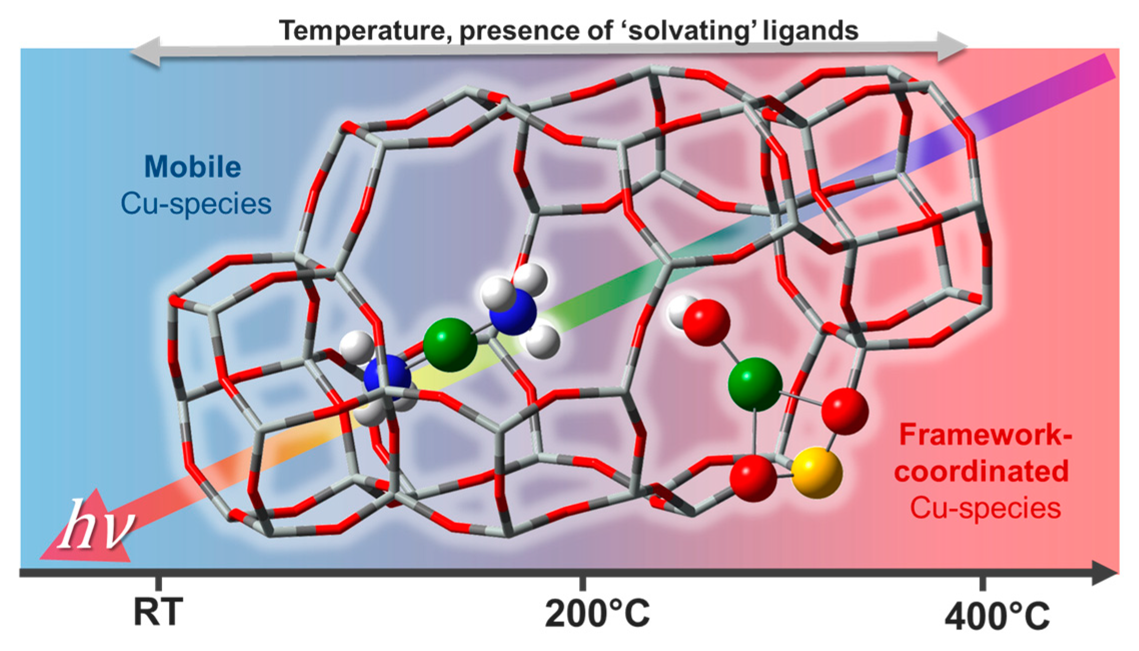
Quantitative determination of the chemical nature and atomic-scale structure of the Cu-species formed without long-rage order in the crystalline zeolite framework after pre-treatment and under reaction conditions represents a key step to keep advancing the field. Cu-zeolites, despite being extensively studied for decades, still present intriguing traits of complexity [89] in connection with the dynamic response of Cu-speciation to the physico-chemical conditions under which the sample is investigated (Figure 13). Recent studies have shown that the active site in low-temperature NH3-SCR catalyst was a mobile Cu-molecular entity that “lives in symbiosis” with the inorganic solid framework [103,104,105,106,107]. Only in high-temperature NH3-SCR regimes, do the mobile Cu-species lose their ligands and find docking sites at the internal walls of the zeolite crystal lattice. These framework-coordinated Cu-species often adopt quite peculiar coordination geometries which are difficult to reproduce in ad hoc synthesized model compounds. Moreover, their nature and redox properties are strongly influenced by compositional characteristics (Si/Al and Cu/Al ratios) of the investigated Cu-zeolite.
In this context, in situ/operando XAS, eventually aided by computational modelling [2,5,6,108], represents an ideal technique to clarify local structure and chemical properties of Cu-species formed [2,4,109,110,111]. Nonetheless, XAS datasets collected in such experiments mostly consist of a mixture of spectroscopic contributions arising from multiple Cu-species, evolving with composition- and condition-dependent concentration profiles. This often hampers quantitative determination of Cu-speciation, hence preventing the possibility to establish robust structure-activity relationships.
To address this limitation, the use of MCR-ALS analysis on large XAS datasets has proven to be extremely effective, enabling quantification of Cu-speciation in Cu-CHA [37,39,40,51,100] and Cu-MOR [38] under conditions relevant to both DMTM and NH3-SCR [89,112,113]. In the following, we will summarize these findings, aiming at highlighting the potential of the MCR/XAS combination to face the characterisation challenge in metal-exchanged zeolites, reveal structure-activity correlations and ultimately decipher reaction mechanisms and nature of the active sites for the targeted processes.
A general note is deserved about how reconstruction ambiguities, discussed in Section 2.2.2, have been managed in the successful research examples reported below for Cu-zeolites. In all the presented cases, multiple XAS datasets collected (i) under the same conditions (temperature profile and reaction feed) on Cu-zeolites with the same topology but different compositional characteristics and/or (ii) under different conditions for the same Cu-zeolite sample were collectively analysed by MCR-ALS. Upon careful selection of the set of samples/experimental protocols, through such “multi-way” MCR-ALS analysis, it was possible to maximize the variance of the global dataset, greatly enhancing the chances to have portions of the dataset characterised by the presence of each PC with concentration close to unit. As shown in Section 2.2.2, in addition to the use of non-negativity constrains for spectral and concentration profiles as well as mass balance condition, this represents an important requirement to drive the reconstruction towards a meaningful solution. If, under the relevant experimental conditions certain Cu-species are still expected to contribute only minorly in the whole dataset, it was shown that the MCR-ALS algorithm can be “guided” by fixing the spectral profile for one or more PCs to those obtained for well-characterised model compounds [37].
A second important aspect regards the a posteriori validation of the obtained solution and of the assignment of each PC to a well-defined Cu-species/sites formed in the zeolite framework. An emerging strategy, pursued, for example, in Reference [51], is the critical comparison of MCR-ALS-retrieved XANES spectra with DFT-assisted simulations, giving access to the theoretical XANES features for an individual structural/electronical configuration of the absorber atom. Moreover, as we will highlight on a case-by-case basis in the following examples, complementary characterisation/testing results consistently obtained in the same study or available in the previous literature, also represent an essential counterpart to assess the validity of the information extracted from MCR analysis of in situ/operando XAS data.
3.1.1. Cu-Speciation in Dehydrated Cu-CHA and Cu-MOR Zeolites and Implications for DMTM
The effect of compositional characteristics on the Cu-speciation in dehydrated Cu-CHA has been extensively debated in the recent literature [89,114]. Two major Cu-sites were suggested to exist with their relative abundance determined by composition, these include: (i) self-reduction-resistant Z2Cu(II) species (Z denotes coordination to zeolite lattice oxygens in the proximity of a charge-balancing Al atom) hosted in 6MRs of the CHA framework at paired 2Al sites and (ii) 1Al Z[Cu(II)OH] complexes stabilized next to isolated 1Al sites preferentially in the 8MR, known to undergo substantial self-reduction to ZCu(I) during pretreatment in inert atmosphere at 400 °C [51,104,115].
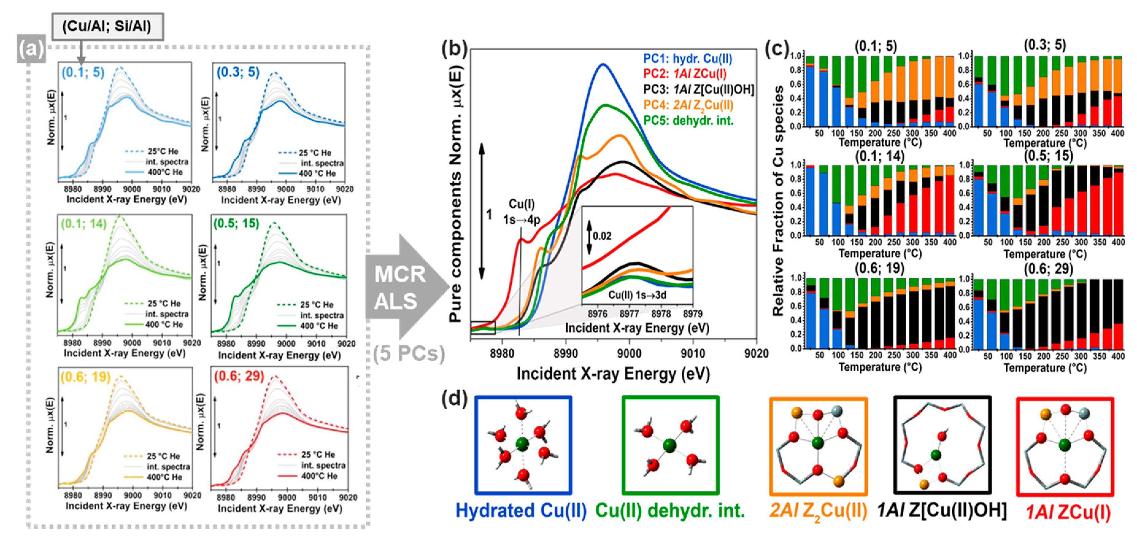
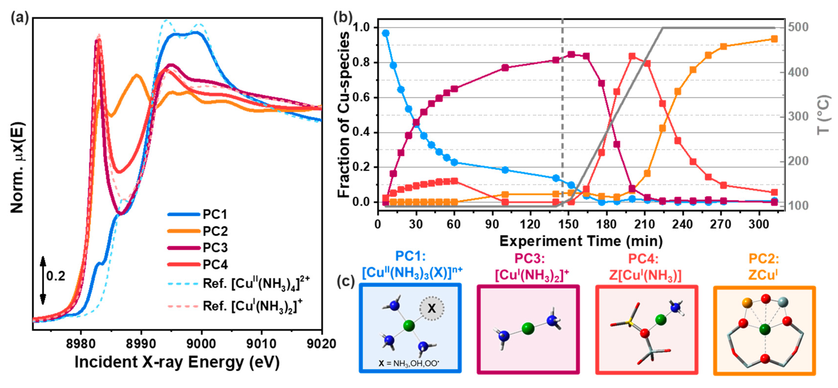
In this context, MCR-ALS analysis (see Section 2.2.2) of temperature- and composition-dependent XANES collected at the BM23 beamline [116] of the European Synchrotron Radiation Facility (ESRF) during thermal pretreatment in He gas flow (Figure 14a) have provided unprecedent quantitative evidences of Cu-speciation in dehydrated Cu-CHA [51]. After PCA of the global XANES dataset, MCR-ALS allowed extracting chemically meaningful spectra and concentration profiles of five pure Cu-species. Based on the spectroscopic fingerprints of each MCR-ALS-retrieved XANES (Figure 14b) and of the correspondent temperature-dependent concentration profiles (Figure 14c), it was possible to reliably assign each pure spectrum to the Cu-species, shown in Figure 14d, also aided by XANES simulations based on the available DFT-optimized geometries for each Cu-species/site.
Framework-interacting Cu-species were formed from mobile Cu(II) aquo-complexes present at RT (PC1) via a four-coordinated Cu(II) dehydration intermediate (PC5), peaking around 130 °C. Then, 1Al Z[Cu(II)OH] (PC3) and 2Al Z2Cu(II) (PC4) species progressively developed, with relative abundance strongly influenced by the Si/Al ratio in the parent zeolite. The Z[Cu(II)OH] peaked around 200 °C and therein started to progressively decrease, in favour of reduced ZCu(I) (PC2) species. Conversely, the Z2Cu(II) sites, dominant at Si/Al = 5, reached a steady population in the 200–300 °C range and remained stable until 400 °C. The Cu-speciation at 400 °C can be described for all samples as a combination of Z[Cu(II)OH]/ZCu(I) and Z2Cu(II) sites, as independently validated by DFT-assisted multi-component EXAFS fits. Remarkably, the self-reducibility level for Z[Cu(II)OH] complexes did not monotonously depend on the Si/Al ratio: the optimal reducibility was observed at Si/Al~15 as was also confirmed by complementary IR spectroscopy of adsorbed N2 [51].
The pure MCR-retrieved XANES spectra shown in Figure 14b further allowed establishing quantitative structure-activity relationships for the stepwise DMTM conversion over a different set of Cu-CHA samples [100]. In particular, the quantitative determination of Cu-speciation by simple XANES linear combination analysis (see Section 2.2.1) using MCR-ALS-derived references indicated that the reducibility after thermal treatment in He gas flow at 500 °C can be used as a descriptor for the methanol productivity in the DMTM process over Cu-CHA.
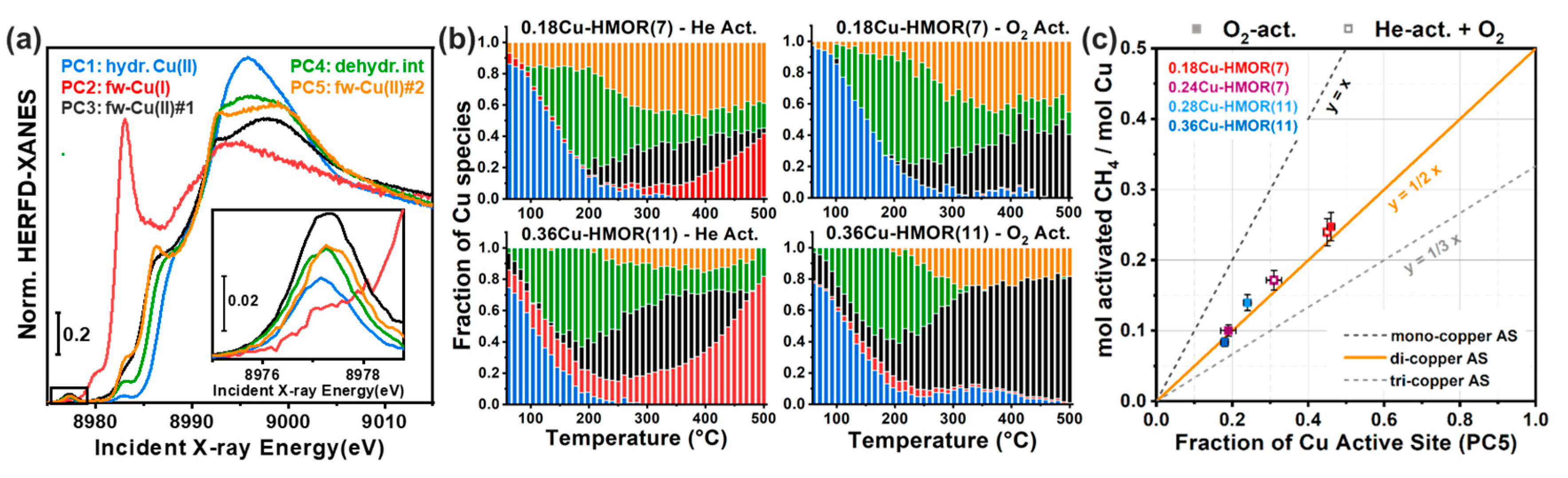
This correlation, together with a number of complementary evidences, indicated that: (i) redox-inert Z2Cu(II) species at 2Al sites were inactive for the DMTM conversion; (ii) Z[Cu(II)OH] complexes at 1Al sites were not directly active but were identified as the precursors to the active sites, plausibly represented by CuxOy moieties formed in the presence of O2. Further insights on the formation of O2-derived species in Cu-CHA were obtained from MCR analysis of high-energy resolution fluorescence-detected XANES data [110,111] collected by means of a crystal spectrometer at an undulator source [37]. Data analysis by MCR–ALS, aided by the enhanced energy-resolution guaranteed by High Energy Resolution Fluorescence Detected (HERFD) XANES, enabled the identification of an additional framework-coordinated Cu(II) species. This component, solely formed in the presence of O2 at temperature >200 °C, is plausibly connected with a CuxOy species and suggested to play a role in the DMTM conversion over Cu-CHA [37].
Another demonstration of the potential of MCR-ALS analysis of HERFD XANES datasets was provided in the context of methane conversion over Cu-MOR. In particular, by correlating XANES-derived information about Cu-speciation during different pretreatments with laboratory activity measurements carried out under consistent conditions, it was possible to unambiguously assess the nuclearity of the DMTM Cu active sites in the investigated Cu-MOR zeolites [38], lively debated in the specialized literature. Temperature-dependent HERFD XANES measurements were performed at the ID26 beamline [110] of the ESRF during thermal treatment in both O2 and He gas flow for two selected Cu-MOR zeolites, showing significantly different DMTM productivities. The global HERFD XANES dataset was analysed by means of PCA and MCR-ALS, identifying 5 PCs with the pure spectra and concentration profiles shown in Figure 15a,b.
These findings for Cu-MOR underpin a similar scenario as previously discussed for Cu-CHA (Figure 14) [51]. Pseudo-octahedral Cu(II) aquo complexes (PC1) undergo partial dehydration to four coordinated Cu(II) dehydration intermediates (PC4). This species reaches maximum concentration around 200 °C, and then gradually converts into two framework-interacting fw-Cu(II) species (PC3, PC5). Among these, fw-Cu(II)#1 (PC3) efficiently undergoes reduction to fw-Cu(I) (PC2) in He gas flow already from 250 °C. Conversely, fw-Cu(II)#2 (PC5) remains stable in He up to 400 °C and is more abundant in the 0.18Cu-HMOR(7) sample, showing the best DMTM performance. All this evidence consistently suggests that fw-Cu(II)#2 should represent the CuxOy active site for the DMTM conversion.
A second stage of the study involved the characterisation of a larger set of Cu-MOR materials by higher-quality HERFD XANES, after the samples were maintained at 500 °C in O2 for 30 min or kept in He flow and subsequently exposed to O2 at the same temperature. The MCR-ALS-retrieved spectra reported in Figure 15a were thus employed as references in LCA of high-quality HERFD XANES scans, to precisely quantify Cu-speciation in this complete set of samples/conditions. Finally, laboratory DMTM activity tests were repeated under exactly the same pretreatment protocols as adopted for HERFD XANES. The resulting yield of CH4 oxidation products per Cu was observed to directly correlate with the abundance of fw-Cu(II)#2, corroborating the assignment of this component to CuxOy active sites (Figure 15c). Here, all the experimental points are observed to match the characteristic trend line for stoichiometric DMTM conversion over a di-copper active site (orange, solid line in Figure 15c), requiring two Cu ions to activate a CH4 molecule.
It is clear that such an accurate Cu speciation-activity correlation would have been out of reach without braiding spectral decomposition techniques, superior energy resolution and careful selection of samples and treatment protocols in order to maximize the variance of the analysed dataset.
3.1.2. Cu-Speciation in Cu-CHA Catalysts under NH3-SCR-Relevant Conditions
As mentioned at the beginning of Section 3.1, the Cu-CHA zeolite represents the catalyst of choice for commercial deNOx applications especially in the automotive sector, to remove polluting nitrogen oxides from the exhaust gases of diesel vehicles via NH3-SCR [89,90,114]. The reaction stoichiometry is given by: 4 NO + 4 NH3 + O2→4 N2 + 6 H2O. Here, ammonia is a key reactant, which is also known to induce profound modifications in the nature of Cu-species present in the catalysts, due to the fact of its high solvation/mobilization ability towards Cu ions [92,105,106,107]. Thus, clarifying nature and thermal stability of Cu-amino-complexes formed inside the CHA zeolite in the presence of ammonia is an important step to clarify certain aspects of the NH3-SCR mechanism.
In this context, PCA and MCR-ALS analysis of XAS data obtained for Cu-CHA during NH3-temperature programmed desorption (TPD, He gas flow) and temperature programmed surface reaction (TPSR, 1% NO/He gas flow) (Figure 16) has provided important insights [39]. Such approach has enabled a much higher level of detail with respect to what would have been possible by LCA using the experimental spectra of model Cu-amino complexes, e.g., [Cu(I)(NH3)2]+ and [Cu(II)(NH3)4]2+ as references.
The MCR-ALS results pointed to the formation of mixed-ligand amino-Cu(II) complexes such as [Cu(II)(NH3)3(OH)]+ (PC1, light blue in Figure 16), starting to desorb NH3 already from 100 °C. Notably, the MCR-ALS retrieved XANES spectrum for these species (Figure 16a) closely resembles the one of [Cu(II)(NH3)4]2+. However, it exhibited broadened features in correspondence of both the rising-edge and while line peaks, consistently with the replacement of one over four NH3 with a different ligand. A key result attained by MCR-ALS analysis was the possibility to deconvolve contributions from mobile [Cu(I)(NH3)2]+ (PC3) and framework-coordinated Z[Cu(I)(NH3)] (PC4) moieties, while allowing to extract the XANES signature of the latter species, difficult to replicate synthetically. As evident in the profiles reported in Figure 16b, the concentration peak of such Z[Cu(I)(NH3)] intermediates preludes to the final NH3 desorption step leading to bare ZCu(I) species (PC2), well matching the dip in NO conversion commonly detected around 350 °C during NH3-SCR over Cu-CHA [117]. This observation could have interesting mechanistic implications: the formation of Z[Cu(I)(NH3)] is envisaged to transiently hamper O2-activation within the SCR cycle, separating low-temperature and high-temperature regimes where O2 is believed to be more efficiently activated over mobile [Cu(I)(NH3)2]+ by transient pair formation [106,107] or over bare ZCu(I) ions, respectively.
The study discussed above focused on in situ XAS experiments, to obtain information relevant to the SCR reaction by separately investigating the interaction of selected reactants with the catalyst. In a more recent report, Clark et al. [40] conjugated time-resolved XAS and MCR-ALS analysis to monitor Cu-CHA under actual operando conditions during NH3-SCR as well as to follow the transient modification in Cu-speciation during fast cut-off/addition of NH3 and NO. Operando Cu K-edge XAS measurements were performed at the SuperXAS beamline of the Swiss Light Source (SLS) [118] in quick-scanning extended X-ray absorption fine structure spectroscopy (QEXAFS) mode, reaching an excellent time-resolution of 500 ms/scan.
The MCR-ALS analysis was simultaneously applied to multiple QEXAFS datasets collected following the cut-off/addition of either NH3 or NO from the reaction mixture at several temperatures [119].
Figure 17a reports the MCR-ALS-retrieved pure spectra for the five components identified during operando QEXAFS experiments, compared with reference Cu K-edge XANES spectra for relevant model compounds (Figure 17b). The comparison corroborated the assignment proposed by the authors. However, it also emphasized the added value of MCR analysis, allowing for instance isolation of the spectral signatures for framework-coordinated Cu(I) and Cu(II) ions, which significantly differ from those of Cu2O and CuO references, in line with previous studies [51,104]. Furthermore, MCR-ALS analysis has provided quantitative evidence about the concentration profiles of the identified spectral components during the different transient experiments performed. With this respect, examples related to NH3 cut-off experiments at 190, 225, 283 and 400 °C are reported in Figure 17c, while Figure 17d reports the correspondent concentrations of NH3 and NO from online mass spectrometry during the same experiments.
In agreement with previous reports [105], the Cu-speciation after equilibration under SCR conditions is strongly influenced by operation temperature. In particular, below 283 °C a significant fraction of “solvated” linear Cu(I) species was observed. Conversely, from 283 °C upward, solvated Cu(I) and Cu(II) species were no longer detected, whereas Cu-speciation was dominated by framework-coordinated Cu ions. Importantly, perturbation of the steady-state SCR conditions by cutting-off NH3 translated into transient modifications in Cu-speciation. In particular, at both 190 and 225 °C, MCR-ALS revealed a transient increase in solvated square planar Cu(II) species immediately after NH3 removal from the gas feed. In parallel, mass spectrometry data (Figure 17d) indicated a transient increase in NO conversion. These findings allowed the authors to support the previously proposed NH3 inhibition effect [119], implying that NH3 locks solvated Cu-ions to Cu(I) species, hampering their re-oxidation to Cu(II) with a consequent decrease the SCR activity in the low-temperature range.
While the interested reader is referred to the original work by Clark et al. for additional chemical insights about NH3-SCR reactivity [40], the selected example well demonstrates the impact of MCR techniques in effectively interpreting the larger and larger spectral datasets collected by quick and dispersive XAS [19,20,118,120,121,122] to boost the time resolution of the technique. Remarkably, a similar approach combining operando QEXAFS and PCA/MCR-ALS analysis has been also recently employed to investigate Pd/Cu-exchanged zeolite Y catalysts for the heterogeneous Wacker oxidation of ethylene [43].
3.2. Shedding Light on Supported Metal Catalysts by XAS Spectral Decomposition Techniques
Transition-metal complexes and low-nuclearity metal-oxo clusters in zeolites discussed in the previous section play an important role in the current scenario of selective redox catalysis [89,123]. Nonetheless, supported metal catalysts remain the most classical and ubiquitously exploited systems in the field of heterogeneous catalysis, for (de)hydrogenation/oxidation reactions, biomass conversion, Fischer-Tropsch and ammonia synthesis, deNOx applications and many other well-established and emerging processes [124,125,126,127]. Also in this context, XAS have been widely employed, to elucidate local structural properties, electronic configuration and reactivity of supported metal/metal-oxide nanoparticles (NPs) [2,128,129]. Careful EXAFS analysis has shown a great potential in the characterisation of such structurally-challenging and dynamic nano-systems, enabling robust determination of statistically-averaged size and shape of the NPs under catalysis-relevant conditions, together with details on compositional distribution (e.g., core/shell, cluster-to-cluster or random alloy) in bimetallic systems [130]. Still, we envisage that spectral decomposition techniques allowing blind source separation of the dataset components [21] will have a significant impact to keep advancing the field, e.g., unlocking the information hidden in subtle variations of the XANES spectra for both the metal and the support components. The few selected examples discussed in the following sections are aimed at supporting these considerations, while demonstrating the potential of XAS spectral decompositions methods alternative to MCR-ALS, widely covered in previous Section 3.1.
Also, in this case, a note is deserved on strategies adopted to mitigate the rotational ambiguity problem. Similarly to what was previously mentioned in Section 3.1, critical comparison with complementary characterisation results is essential: the pioneering study by Fernandez-Garcia et al. [14] about zeolite-supported bimetallic PdCu particles using ITTFA (Section 3.2.1) refers for instance to H2-TPR studies for cross-validation of the in situ XANES results. For more recent applications involving the TM matrix approach, both the selected examples (Section 3.2.2 and Section 3.2.3) emphasize the importance of identifying and applying suitable constrains in order to reduce as much as possible the number of free parameters (i.e., user-controlled sliders in the PyFitIt implementation). With this respect, boundaries conditions can be used, e.g., setting as pure spectra the first and/or the last experimental scans in the dataset. In parallel, normalization of the extracted spectral profiles can be employed as an additional strategy to reduce the number of free parameters. For a detailed description on how these constraints are mathematically realized, the interested reader is referred to Reference [65].
3.2.1. Phase Behaviour of a Pd-Cu Bimetallic Catalyst during H2-TPR
Fernandez-Garcia et al. employed for the first time in the analysis of XANES data a self-modelling approach, the ITTFA method (see Section 2.2.2), in order to study the phase speciation in Pd-Cu bimetallic catalysts during TPR in H2 [14]. The authors analysed two bimetallic samples, namely, PdCu50 (1% Pd and 0.5% Cu) and PdCu25 (1% Pd and 0.25% Cu) supported on the K-exchanged form of an L zeolite (KL) [14]. The XANES-TPR experiments were performed in a controlled-atmosphere cell, heating the sample at a rate of 5 K/min from RT to 773 K in flowing H2/He (5 vol % H2). The resulting datasets are reported in Figure 18a,b.
The application of PCA on both datasets and the further study of the derived statistical estimators, employed to identify the correct number of chemical species affecting the dataset, revealed the presence of three principal components. In particular, the authors analysed the variance associated to each component together with the dataset IND and F-Test. Therein, they underlined a certain degree of ambiguity related on the number of PCs to consider. In particular, while the variance analysis and the F-Test suggested the existence of three components, the Malinowski IND factor showed a minimum in correspondence of the fourth component. This problem was solved visually examining the shape and intensity of this last component, which appeared dominated principally by noise and, for this reason, excluded from the subsequent analysis. Having identified the correct number of pure components characterising the XANES datasets, the authors applied ITTFA (see Section 2.2.2) to convert the three abstract spectral profiles in the corresponding set of spectroscopically interpretable pure XANES. The retrieved pure spectral profiles together with their related concentration values during H2-TPR experiments are shown in Figure 19.
Analysing Figure 19, it is interesting to observe that two species, (1) and (2), are simultaneously present at the beginning of the H2-TPR process (after the calcination of the catalysts [14]) while only one, (3), is required to describe the final state of the system.
The shape of the spectrum (1) in Figure 19 corresponds to a Cu(II) species, having a square-planar coordination in perfect agreement with the Cu(II) coordination symmetry proper of Cu-Pd mixed oxides. Moreover, it is worth noting in Figure 19c,d, that the concentration profiles of this species, for both the samples, did not show a characteristic reduction temperature, suggesting the presence of a solid solution of the Cu component in the PdO host matrix. The second species, whose concentration was higher for the PdCu25 sample, possesses a XANES spectrum ascribable to Cun+ cations exchanged into L-zeolite positions [131]. In order to obtain deeper insights on this species, the authors tried to compare it quantitatively with two reference spectra corresponding to CuO and Cu2O oxides. However, the analysis of the SPOIL factors (see also Section 2.2.1) indicated that it did not correspond to either of the two Cu oxides (SPOIL > 6 in both cases). This finding is ultimately in agreement with the results discussed in the previous Section 3.1, highlighting how framework-coordinated Cu ions in zeolites adopt peculiar coordination geometries, difficultly reproduced by model compounds such as CuO and Cu2O. Finally, during the reduction process, no intermediate compounds were observed. Both the Cu species yielded to a third component, species (3), which was assigned to metallic Cu(0), occurring in the form proper of the Cu-Pd alloy.
3.2.2. Pd Carbide and Hydride Formation in Supported Pd-Catalysts
Supported Pd-based catalysts are massively employed at the industrial scale for selective hydrogenation of hydrocarbons [132,133]. Under reactions conditions, metallic Pd may convert into Pd-hydride (Pd-H) or Pd-carbide (Pd-C) phases, with consequent modifications in the activity and selectivity of the catalysts [134]. Upon formation of such species, H or C atoms enter the fcc lattice of metal Pd, occupying interstitial octahedral sites and causing elongation of the lattice parameter detectable by PXRD and EXAFS [135,136]. Nonetheless, both the techniques have been shown to possess poor sensitivity in discriminating among Pd-H and Pd-C phases which render them rather ineffective in pinpointing the active Pd-phase under reaction conditions. With this respect, more accurate information can be accessed by probing the modification in the electronic states due to the mixing of Pd orbitals with those of H/C ligands upon formation of Pd-H/Pd-C bonds. Here, XPS [137,138] and Pd L-edges studies [139,140] using low-energy X-rays have provided important insights. However, the possibility to obtain equivalent information by hard X-ray XANES at Pd K-edge, much more suited for in situ/operando experiments at ambient pressure, have been also demonstrated [141]. In this context, rather limited spectral variance across the obtained datasets was often observed, which put a prize on advanced data analysis methods capable to robustly capture the underlying modifications in Pd-speciation. Beside differential ΔXANES approaches [55,141], statistical analysis and spectral decomposition methods can offer viable solutions in the interpretation of these data.
With this respect, Bugaev et al. [55] investigated the formation and decomposition of the Pd-C phase in the bulk and at the surface of 2.6 nm Pd NPs supported on wood-based activated carbon upon their exposure to acetylene, hydrogen and their mixtures, by means of Pd K-edge XAS measurements carried out at the BM31 beamline [142] of the ESRF.
Initially, the sample was activated in pure H2 at 120 °C, successively evacuated, and cooled down to 100 °C to obtain the spectrum of the clean NPs (pure Pd metallic phase). Then, it was exposed to a mixture of acetylene and hydrogen with partial pressures of 350 and 650 mbar, respectively, resulting in the formation of Pd-H species. In order to form the Pd-C phase, the sample was subsequently exposed to pure acetylene, and three consecutive XAS spectra were collected. The stability and reversibility of the carbide phase were checked first by evacuation down to 10−3 mbar at 100 °C and then by treatment in hydrogen (1000 mbar at 100 °C) and subsequent evacuation, that caused the partial removal of Pd-C species. Then, the sample was exposed again to pure acetylene at 100 °C determining a further grown of the carbide phase. The resulting dataset, shown in Figure 20a, consisted in only ten spectra, but acquired uniformly during the entire evolution of the metal, hydride and carbide phases. Here, PCA led to the identification of three pure Pd-species, as consistently supported by all the employed statistical estimators, namely, scree plot, IE, IND and F-test. Afterwards, the retrieved three pure components and their related weights were modified on the basis of the TM approach (see Section 2.2.2) employing the non-negativity constraint for the normalized spectral and concentration profiles as well as the mass balance condition. Moreover, because the first spectrum of the dataset corresponded to the pure Pd metal phase, it was safely fixed as a pure component, determining the reduction of the elements of the transformation matrix from six to four [65].
The retrieved pure spectra are reported in Figure 20b, while Figure 20c shows the correspondent concentration profiles. They were assigned to pure Pd metal NPs, Pd-hydride and Pd-carbide phases, for the 1st, 2nd and 3rd components, respectively.
It is possible to see from the spectral and concentration profiles reported in Figure 20b,c the initial state is represented by pure metallic Pd. Then, exposing the sample to a mixture of acetylene and hydrogen at 100 °C (with the partial pressures described before) it is possible to assist to the Pd-H phase formation and to the subsequent hydrogenation of acetylene to ethylene. After the exposure to pure acetylene, the pure metallic and carbide phases coexist in the investigated Pd-NPs. At longer time scales, the concentration of the metallic phase shows a decreasing trend, while the opposite behaviour is observed for the carbide one. After cleaning in hydrogen, a drop in the Pd-component and an increase of the pure metallic phase are visible. It is interesting to note that the Pd-component was not observed, in its pure state, in any of the investigated experimental conditions. Moreover, it is remarkable that the EXAFS of the Pd-component virtually coincided with that of the hydride, meaning that both phases have similar interatomic distances as showed by complementary PXRD studies [135].
3.2.3. Tracking the Ce-Speciation in Pt/CeO2 Catalysts under Redox Conditions
Noble metals on redox-active CeO2 supports are largely employed in the automotive sector to clean vehicles exhaust gases from polluting products such as CO, NOx and unreacted hydrocarbons. In relation with their application in gas aftertreatment systems, these catalysts naturally operate under rapid oscillations of the gas feed composition [143], making transient XAS experiments particularly suited to determine and correlate reduction/oxidation kinetics of both noble-metal NPs and ceria support.
To this aim, Guda et al. [65,144] employed, at the SuperXAS beamline of the SLS, a setup for fluorescence-detected XAS with sub-second time resolution to track Ce-speciation in 1.5 wt% Pt/CeO2 catalysts while cycling CO and O2 gas feeds. The sample was sieved to 100–150 μm grain size and placed into an in situ plug-flow reactor cell [145]. Afterwards, the reactor was connected to gas lines devoted to reductive (5% CO in argon) and oxidative (21% O2 in argon) gas feeds; fast electro-valves allowed quick switching between these two mixtures. The study involved XAS data collection at both Pt L3- and Ce L3-edge; hereafter, we focus on the latter dataset, addressing the response of the CeO2 support. Figure 21a shows the set of experimental spectra, recorded during two redox cycles at 26 °C and 90 °C, consisting into 120 s of reduction by CO gas flow followed by 60 s of oxidation in O2. These cycles were repeated for every energy point of the spectrum, selected by the monochromator; in each point, the Ce L3 fluorescence signal was recorded with 0.3 s time resolution, ultimately resulting in 1103 Ce L3 XANES spectra.
The differences between subsequent spectra are hardly visible from simple qualitative analysis of the dataset, as it can be noted in Figure 21a. Thus, quantitative analysis of the PCs was applied to clarify the number of pure components in the set of spectra and their concentrations profiles. PCA performed on the raw fluorescence-detected data indicated the presence of two components affecting the dataset; all the statistical estimators (scree plot, IE, IND, and F-test) suggested the same number of PCs. Similar to what was done in the previously discussed example, also in this case the TM approach (see Section 2.2.2) was employed to model the abstract spectra and concentrations, starting from an initial transformation matrix consisting of four elements. Imposing the normalization of the components, the number of its free parameters was reduced to two. Afterwards, these elements were moved in order to guarantee the non-negativity of the spectra and concentration values, as well as the mass balance condition, yielding the solution shown in Figure 21b,c.
Kinetic curves showed in Figure 21c contain important information about the catalytic properties of the system. First, it is possible to directly estimate the concentration of active oxygen atoms which are released from ceria lattice at the two investigated temperatures of 26 and 90 °C. Indeed, each released oxygen leaves two electrons in the system, which reduce two ceria atoms from Ce(IV) to Ce(III). The amount of lattice oxygen that can be extracted in CO atmosphere from the ceria support in the investigated Pt/CeO2 system increases six times upon temperature increase. Another important feature is that at 26 °C ceria is not fully oxidized in the O2 atmosphere and a small fraction of Ce(III) atoms is constantly present in the lattice, as also indicated by other methods [146]. Finally, the time-dependent concentrations can be further used to calculate kinetic constants of the system which are important to understand the microscopic origin of the catalytic behaviour of the ceria-based catalysts [144].
4. Conclusions and Perspectives
In summary, in this work we introduced and described in detail different methods employed to decompose a XAS data matrix in a set of pure spectral and concentration profiles referring to the different species present in the measured chemical mixture. All the decomposition approaches are initially based on the analysis of the principal components, representing an essential and well-established procedure to understand the number of chemical species affecting the dataset.
Selection of the most appropriate methods among the various MCR approaches described in the previous sections should be driven by the degree of variation of the dataset. In particular, the TM method demonstrated to be useful when the XAS data matrix only shows small changes in its spectral features. Conversely, the ITTFA and the MCR-ALS routines appear to be more suitable for those datasets that are characterised by several components and affected by larger variations.
In all cases, the definition of a good set of constraints involving also the possibility to combine the chemical information gained by different theoretical and experimental techniques (see below) leads the routines toward a feasible and meaningful solution, delivering accurate information which would be difficult, if not impossible, to get otherwise by the simple qualitative analysis of the XAS spectra.
Since their first appearance in the context of XAS data analysis, PCA and MCR approaches rapidly spread across several research areas. These methods imposed as essential tools for in-depth analysis of datasets acquired during time-resolved experiments, as illustrated by the examples discussed in this review with an emphasis on in situ/operando characterisation in catalysis. Here, thanks to the advent of third-generation synchrotron radiation facilities, an accurate description of the chemical species involved in a process can be achieved with resolution down to sub-ms timescale, allowing to capture even short-lived reaction intermediates [33]. Applications of these methods to space-resolved XAS [147] have been also reported, especially in the fields of environmental/earth science and cultural heritage [148,149]. With this respect, we envisage important developments also in catalysis-related research, to guide data analysis in advanced spectroscopic applications able to reveal and track heterogeneities of individual catalyst particles in both the time and space domain [150].
However, as shown before, the main bottleneck of these techniques remains connected with the ambiguity of the identified solution. Indeed, in most cases, only the presence of a strong set of constraints can drive the MCR algorithms towards a chemically/physically interpretable result. In this respect, it is worth noting that the employment of certain constraints clearly depends on the knowledge of the system under study, which sometimes is challenging to access, if not ultimately precluded.
In order to overcome this problem, different theoretical and experimental multi-technique approaches have been employed together with XAS analysis of the sample under study. For instance, Smolentsev et al. [1] conjugated the TM decomposition approach with a XANES interpolation-based method to shed light on a reaction involving a methylrhenium trioxide catalyst. In this work, the authors showed that it is possible to remove the ambiguity associated to the MCR solution by minimizing an objective function depending on the elements of the transformation matrix and on the structural parameters characterising the XANES interpolated spectra. Similarly, Tavani et al. [32] analysed a set of energy-dispersive XANES spectra obtained on a class of non-heme iron complexes using again the TM method. Afterwards, the isolated spectra were quantitatively characterised by full multiple scattering calculations using the MXAN code [151,152]. This procedure allowed retrieving mechanistic information about the room-temperature reaction of Fe(II)(tris(2-pyridylmethyl)amine) with peracetic acid in CH3CN as well as with native non-derivatized TPA substrate.
Noteworthy are the joined applications of the MCR algorithm on sets of data referring to different experimental techniques employed to track a determined reaction. Notably, EPR, XANES/EXAFS, UV-Vis and ATR-IR spectroscopic methods were employed for the first time in the same experimental setup by Rabeah et al. [31] for the investigation of unclear aspects connected to the selective aerobic oxidation mechanism of benzyl alcohol by a Cu/TEMPO catalytic system. The authors showed that the MCR-ALS approach executed on two sets of XAS and UV-Vis data acquired simultaneously during the same experiment was able to identify a set of three pure species, among which only one was not EPR-silent.
Taken together, these pioneering examples outline two important development routes to further improve reliability and applicability of MCR-based approaches, including (i) theory-driven constrains or/and output validation and (ii) combined analysis of multi-technique datasets, possibly acquired in a quasi-simultaneous fashion and unlocking complementary information on the investigated system/process.
Finally, it is worth noting that, to the best of our knowledge, MCR algorithms have never been applied to the analysis of soft X-ray Near Edge X-ray Absorption Fine Structure (NEXAFS) spectra, to date. However, much valuable information on the physico-chemical properties of the system under study could emerge combining NEXAFS measurements of deep-core K- and L-edge spectra. In particular, NEXAFS analysis would be uniquely suited not only for studying light elements (O, C, N, etc.) but also for the parallel investigation of transition metals, which plays a key role in a multitude of catalytic reactions [153,154]. In fact, since the XANES region is governed by the dipole selection rules, the d-shell properties of the first-row transition metals would be best probed by the L2,3 absorption edges [155,156]. Moreover, while NEXAFS measurement are typically carried out under high-vacuum conditions, in the last decade innovative experimental layouts and cell design have made possible in situ/operando studies under gaseous environments at atmospheric pressure [153,157,158]. These instrumental advances together with the competitive time-resolution achievable at dedicated beamlines are paving the way to previously unexplored characterisation opportunities, e.g., in the fields of catalysis and gas adsorption/sensing [159,160,161,162]. In this context, also considering the remarkably high spectral variance and sharp resonances commonly characterising in situ NEXAFS datasets, we expect a rapid growth in the use of statistical and spectral decomposition techniques.
The major problem connected with the application of MCR approaches to NEXAFS analysis can be identified in the complex data treatment procedure which is employed to properly correct and normalize the acquired set of data [163]. The presence of several edges sited at close distances in energy can make the data normalization protocols well established for hard X-ray XAS sometimes difficult or even impossible to realize. In addition, due to the presence of a gas atmosphere, if in situ NEXAFS measurements are performed in total electron yield (TEY) mode, it is probable that the spectral background would not be linear [158]. Nonetheless, different codes specifically designed for the analysis of soft XAS data have been recently developed [163,164], allowing to overcome these issues and making the application of MCR approaches to this typology of data soon a reality.
Author Contributions
Conceptualization, writing, review and editing, A.M. and E.B. All authors have read and agreed to the published version of the manuscript.
Funding
The APC was funded by project n. 2017KKP5ZR PRIN-2017 MOSCATo (Cutting-edge X-ray methods and models for the understanding of surface site reactivity in heterogeneous catalysts and sensors).
Acknowledgments
We are grateful to E. Groppo and M. Carosso for insightful discussions about Pt/Al2O3 catalysts and to S. Bordiga and G. Ricchiardi for their support and advice. We acknowledge many colleagues at synchrotron sources for their competent and friendly help during several XAS experiments, in particular, at the ESRF: K.A. Lomachenko (ID24/BM23), P. Glatzel (ID26), A. Longo (ID20), W. Van Beek (BM31); at the Elettra synchrotron: L. Braglia, P. Torelli (APE-HE). A.M. thanks A.A. Guda, S.A. Guda, A L. Bugaev, M.A. Soldatov and A.V. Soldatov (The Smart Materials Research Institute, Southern Federal University) and F. Tavani and P. D’Angelo (Sapienza, Università di Roma) for fruitful collaborations on method developments. We are deeply indebted to C. Lamberti for showing us the direction, being an amazing mentor and a brilliant guide.
Conflicts of Interest
The authors declare no conflict of interest.
References
- Smolentsev, G.; Guilera, G.; Tromp, M.; Pascarelli, S.; Soldatov, A.V. Local structure of reaction intermediates probed by time-resolved X-ray absorption near edge structure spectroscopy. J. Chem. Phys. 2009, 130, 174508. [Google Scholar] [CrossRef] [PubMed]
- Bordiga, S.; Groppo, E.; Agostini, G.; van Bokhoven, J.A.; Lamberti, C. Reactivity of surface species in heterogeneous catalysts probed by in situ X-ray absorption techniques. Chem. Rev. 2013, 113, 1736–1850. [Google Scholar] [CrossRef] [PubMed] [Green Version]
- Mino, L.; Agostini, G.; Borfecchia, E.; Gianolio, D.; Piovano, A.; Gallo, E.; Lamberti, C. Low-dimensional systems investigated by X-ray absorption spectroscopy: A selection of 2D, 1D and 0D cases. J. Phys. D Appl. Phys. 2013, 46, 72. [Google Scholar] [CrossRef]
- Garino, C.; Borfecchia, E.; Gobetto, R.; Salassa, L.; van Bokhoven, J.A.; Lamberti, C. Determination of the electronic and structural configuration of coordination compounds by synchrotron-radiation techniques. Coord. Chem. Rev. 2014, 277–278, 130–186. [Google Scholar] [CrossRef] [Green Version]
- Rehr, J.J.; Ankudinov, A.L. Progress in the theory and interpretation of XANES. Coord. Chem. Rev. 2005, 249, 131–140. [Google Scholar] [CrossRef]
- Joly, I.; Grenier, S. Theory of X-ray Absorption Near Edge Structure. In X-ray Absorption and X-ray Emission Spectroscopy: Theory and Application; van Bokhoven, J.A., Lamberti, C., Eds.; John Wiley & Sons: Hoboken, NJ, USA, 2016; pp. 73–98. [Google Scholar]
- Guda, A.A.; Guda, S.A.; Lomachenko, K.A.; Soldatov, M.A.; Pankin, I.A.; Soldatov, A.V.; Braglia, L.; Bugaev, A.L.; Martini, A.; Signorile, M.; et al. Quantitative structural determination of active sites from in situ and operando XANES spectra: From standard ab initio simulations to chemometric and machine learning approaches. Catal. Today 2019, 336, 3–21. [Google Scholar] [CrossRef]
- Sayers, D.E.; Stern, E.A.; Lytle, F.W. New Technique for Investigating Noncrystalline Structures: Fourier Analysis of the Extended X-Ray Absorption Fine Structure. Phys. Rev. Lett. 1971, 27, 1204–1207. [Google Scholar] [CrossRef]
- Penner-Hahn, J.E. X-ray absorption spectroscopy in coordination chemistry. Coord. Chem. Rev. 1999, 190-192, 1101–1123. [Google Scholar] [CrossRef]
- Rehr, J.J.; Albers, R.C. Theoretical approaches to X-ray absorption fine structure. Rev. Mod. Phys. 2000, 72, 621–654. [Google Scholar] [CrossRef]
- Koningsberger, D.C.; Ramaker, D.E. Applications of X-ray Absorption Spectroscopy in Heterogeneous Catalysis: EXAFS, Atomic XAFS, and Delta XANES. In Handbook of Heterogeneous Catalysis; Wiley-VCH Verlag GmbH & Co. KGaA: Weinheim, Germany, 2008; pp. 774–803. [Google Scholar] [CrossRef]
- Meitzner, G. In Situ XAS Characterization of Heterogeneous Catalysts. In In-Situ Spectroscopy in Heterogeneous Catalysis; Wiley-VCH Verlag: Weinheim, Germany, 2004; pp. 179–194. [Google Scholar] [CrossRef]
- Lamberti, C.; van Bokhoven, J.A. X-Ray Absorption and Emission Spectroscopy for Catalysis. In X-ray Absorption and X-ray Emission Spectroscopy: Theory and Application; John Wiley & Sons: Hoboken, NJ, USA, 2016; pp. 351–383. [Google Scholar] [CrossRef]
- Fernandez-Garcia, M.; Alvarez, C.M.; Haller, G.L. XANES-TPR Study of Cu-Pd Bimetallic Catalysts: Application of Factor Analysis. J. Phys. Chem. 1995, 99, 12565–12569. [Google Scholar] [CrossRef]
- Voronov, A.; Urakawa, A.; van Beek, W.; Tsakoumis, N.E.; Emerich, H.; Rønning, M. Multivariate curve resolution applied to in situ X-ray absorption spectroscopy data: An efficient tool for data processing and analysis. Anal. Chim. Acta 2014, 840, 20–27. [Google Scholar] [CrossRef] [PubMed] [Green Version]
- La Fontaine, C.; Belin, S.; Barthe, L.; Roudenko, O.; Briois, V. ROCK: A Beamline Tailored for Catalysis and Energy-Related Materials from ms Time Resolution to µm Spatial Resolution. Synchrotron Radiat. News 2020, 33, 20–25. [Google Scholar] [CrossRef]
- Błachucki, W.; Hoszowska, J.; Dousse, J.-C.; Kayser, Y.; Stachura, R.; Tyrała, K.; Wojtaszek, K.; Sá, J.; Szlachetko, J. High energy resolution off-resonant spectroscopy: A review. Spectrochim. Acta B 2017, 136, 23–33. [Google Scholar] [CrossRef] [Green Version]
- Błachucki, W.; Szlachetko, J.; Hoszowska, J.; Dousse, J.C.; Kayser, Y.; Nachtegaal, M.; Sá, J. High Energy Resolution Off-Resonant Spectroscopy for X-ray Absorption Spectra Free of Self-Absorption Effects. Phys. Rev. Lett. 2014, 112, 173003. [Google Scholar] [CrossRef]
- Nachtegaal, M.; Müller, O.; König, C.; Frahm, R. QEXAFS: Techniques and Scientific Applications for Time-Resolved XAS. In X-ray Absorption and X-ray Emission Spectroscopy: Theory and Application; John Wiley & Sons: Hoboken, NJ, USA, 2016; pp. 155–183. [Google Scholar] [CrossRef]
- Mathon, O.; Kantor, I.; Pascarelli, S. Time-Resolved XAS Using an Energy Dispersive Spectrometer: Techniques and Applications. In X-ray Absorption and X-ray Emission Spectroscopy: Theory and Application; John Wiley & Sons: Hoboken, NJ, USA, 2016; pp. 185–212. [Google Scholar] [CrossRef]
- Timoshenko, J.; Frenkel, A.I. “Inverting” X-ray Absorption Spectra of Catalysts by Machine Learning in Search for Activity Descriptors. ACS Catal. 2019, 9, 10192–10211. [Google Scholar] [CrossRef]
- Carvalho, H.W.P.; Pulcinelli, S.H.; Santilli, C.V.; Leroux, F.; Meneau, F.; Briois, V. XAS/WAXS Time-Resolved Phase Speciation of Chlorine LDH Thermal Transformation: Emerging Roles of Isovalent Metal Substitution. Chem. Mater. 2013, 25, 2855–2867. [Google Scholar] [CrossRef]
- Kränzlin, N.; Staniuk, M.; Heiligtag, F.J.; Luo, L.; Emerich, H.; van Beek, W.; Niederberger, M.; Koziej, D. Rationale for the crystallization of titania polymorphs in solution. Nanoscale 2014, 6, 14716–14723. [Google Scholar] [CrossRef]
- Caetano, B.L.; Briois, V.; Pulcinelli, S.H.; Meneau, F.; Santilli, C.V. Revisiting the ZnO Q-dot Formation Toward an Integrated Growth Model: From Coupled Time Resolved UV–Vis/SAXS/XAS Data to Multivariate Analysis. J. Phys. Chem. C 2017, 121, 886–895. [Google Scholar] [CrossRef]
- Conti, P.; Zamponi, S.; Giorgetti, M.; Berrettoni, M.; Smyrl, W.H. Multivariate Curve Resolution Analysis for Interpretation of Dynamic Cu K-Edge X-ray Absorption Spectroscopy Spectra for a Cu Doped V2O5 Lithium Battery. Anal. Chem. 2010, 82, 3629–3635. [Google Scholar] [CrossRef]
- Mullaliu, A.; Conti, P.; Aquilanti, G.; Plaisier, J.R.; Stievano, L.; Giorgetti, M. Operando XAFS and XRD Study of a Prussian Blue Analogue Cathode Material: Iron Hexacyanocobaltate. Condens. Matter 2018, 3, 36. [Google Scholar] [CrossRef] [Green Version]
- Fehse, M.; Bessas, D.; Darwiche, A.; Mahmoud, A.; Rahamim, G.; La Fontaine, C.; Hermann, R.P.; Zitoun, D.; Monconduit, L.; Stievano, L.; et al. The Electrochemical Sodiation of FeSb2: New Insights from Operando 57Fe Synchrotron Mössbauer and X-ray Absorption Spectroscopy. Batter. Supercaps 2019, 2, 66–73. [Google Scholar] [CrossRef] [Green Version]
- Fehse, M.; Iadecola, A.; Sougrati, M.T.; Conti, P.; Giorgetti, M.; Stievano, L. Applying chemometrics to study battery materials: Towards the comprehensive analysis of complex operando datasets. Energy Storage Mater. 2019, 18, 328–337. [Google Scholar] [CrossRef]
- Eveillard, F.; Gervillié, C.; Taviot-Guého, C.; Leroux, F.; Guérin, K.; Sougrati, M.T.; Belin, S.; Delbègue, D. Unravelling lithiation mechanisms of iron trifluoride by operando X-ray absorption spectroscopy and MCR-ALS chemometric tools. New J. Chem. 2020, 44, 10153–10164. [Google Scholar] [CrossRef]
- Vantelon, D.; Davranche, M.; Marsac, R.; La Fontaine, C.; Guénet, H.; Jestin, J.; Campaore, G.; Beauvois, A.; Briois, V. Iron speciation in iron–organic matter nanoaggregates: A kinetic approach coupling Quick-EXAFS and MCR-ALS chemometrics. Environ. Sci. Nano 2019, 6, 2641–2651. [Google Scholar] [CrossRef]
- Rabeah, J.; Briois, V.; Adomeit, S.; La Fontaine, C.; Bentrup, U.; Brückner, A. Multivariate Analysis of Coupled Operando EPR/XANES/EXAFS/UV–Vis/ATR-IR Spectroscopy: A New Dimension for Mechanistic Studies of Catalytic Gas-Liquid Phase Reactions. Chem. Eur. J. 2020, 26, 7395–7404. [Google Scholar] [CrossRef]
- Tavani, F.; Martini, A.; Capocasa, G.; Di Stefano, S.; Lanzalunga, O.; D’Angelo, P. Direct mechanistic evidence for a non-heme complex reaction through a multivariate XAS analysis. Inorg. Chem. 2020, 59, 9979–9989. [Google Scholar] [CrossRef] [PubMed]
- Cassinelli, W.H.; Martins, L.; Passos, A.R.; Pulcinelli, S.H.; Santilli, C.V.; Rochet, A.; Briois, V. Multivariate curve resolution analysis applied to time-resolved synchrotron X-ray Absorption Spectroscopy monitoring of the activation of copper alumina catalyst. Catal. Today 2014, 229, 114–122. [Google Scholar] [CrossRef]
- Hong, J.P.; Marceau, E.; Khodakov, A.Y.; Gaberova, L.; Griboval-Constant, A.; Girardon, J.S.; La Fontaine, C.; Briois, V. Speciation of Ruthenium as a Reduction Promoter of Silica-Supported Co Catalysts: A Time-Resolved in Situ XAS Investigation. ACS Catal. 2015, 5, 1273–1282. [Google Scholar] [CrossRef]
- Rochet, A.; Baubet, B.; Moizan, V.; Devers, E.; Hugon, A.; Pichon, C.; Payen, E.; Briois, V. Intermediate Species Revealed during Sulfidation of Bimetallic Hydrotreating Catalyst: A Multivariate Analysis of Combined Time-Resolved Spectroscopies. J. Phys. Chem. C 2017, 121, 18544–18556. [Google Scholar] [CrossRef]
- Barzan, C.; Piovano, A.; Braglia, L.; Martino, G.A.; Lamberti, C.; Bordiga, S.; Groppo, E. Ligands Make the Difference! Molecular Insights into CrVI/SiO2 Phillips Catalyst during Ethylene Polymerization. J. Am. Chem. Soc. 2017, 139, 17064–17073. [Google Scholar] [CrossRef]
- Martini, A.; Alladio, E.; Borfecchia, E. Determining Cu-Speciation in the Cu-CHA Zeolite Catalyst: The Potential of Multivariate Curve Resolution Analysis of In Situ XAS Data. Top. Catal. 2018, 61, 1396–1407. [Google Scholar] [CrossRef]
- Pappas, D.K.; Martini, A.; Dyballa, M.; Kvande, K.; Teketel, S.; Lomachenko, K.A.; Baran, R.; Glatzel, P.; Arstad, B.; Berlier, G.; et al. The Nuclearity of the Active Site for Methane to Methanol Conversion in Cu-Mordenite: A Quantitative Assessment. J. Am. Chem. Soc. 2018, 140, 15270–15278. [Google Scholar] [CrossRef] [PubMed]
- Borfecchia, E.; Negri, C.; Lomachenko, K.A.; Lamberti, C.; Janssens, T.V.W.; Berlier, G. Temperature-dependent dynamics of NH3-derived Cu species in the Cu-CHA SCR catalyst. React. Chem. Eng. 2019, 4, 1067–1080. [Google Scholar] [CrossRef]
- Clark, A.H.; Nuguid, R.J.G.; Steiger, P.; Marberger, A.; Petrov, A.W.; Ferri, D.; Nachtegaal, M.; Kröcher, O. Selective Catalytic Reduction of NO with NH3 on Cu-SSZ-13: Deciphering the Low and High-temperature Rate-limiting Steps by Transient XAS Experiments. ChemCatChem 2020, 12, 1429–1435. [Google Scholar] [CrossRef]
- Passos, A.R.; La Fontaine, C.; Pulcinelli, S.H.; Santilli, C.V.; Briois, V. Quick-EXAFS and Raman monitoring of activation, reaction and deactivation of NiCu catalysts obtained from hydrotalcite-like precursors. Phys. Chem. Chem. Phys. 2020, in press. [Google Scholar] [CrossRef] [PubMed]
- Nikulshina, M.; Blanchard, P.; Lancelot, C.; Griboval-Constant, A.; Marinova, M.; Briois, V.; Nikulshin, P.; Lamonier, C. Genesis of active phase in MoW/Al2O3 hydrotreating catalysts monitored by HAADF and in situ QEXAFS combined to MCR-ALS analysis. Appl. Catal. B: Environ. 2020, 269, 118766. [Google Scholar] [CrossRef]
- Imbao, J.; van Bokhoven, J.A.; Clark, A.; Nachtegaal, M. Elucidating the mechanism of heterogeneous Wacker oxidation over Pd-Cu/zeolite Y by transient XAS. Nat. Commun. 2020, 11, 1118. [Google Scholar] [CrossRef] [Green Version]
- Demmel, J.; Gu, M.; Eisenstat, S.; Slapnicar, I.; Veselic, K.; Drmac, Z. Computing the singular value decomposition with high relative accuracy. Linear Alg. Appl. 1999, 299, 21–80. [Google Scholar] [CrossRef]
- Calvin, S. XAFS for Everyone; CRC Press: Boca Raton, FL, USA, 2013. [Google Scholar]
- Carosso, M.; Vottero, E.; Lazzarini, A.; Morandi, S.; Manzoli, M.; Lomachenko, K.A.; Ruiz, M.J.; Pellegrini, R.; Lamberti, C.; Piovano, A.; et al. Dynamics of Reactive Species and Reactant-Induced Reconstruction of Pt Clusters in Pt/Al2O3 Catalysts. ACS Catal. 2019, 9, 7124–7136. [Google Scholar] [CrossRef]
- Malinowski, E.R. Factor Analysis in Chemistry; Wiley: Weinheim, Germany, 2002. [Google Scholar]
- Brereton, R.G. Chemometrics: Data Analysis for the Laboratory and Chemical Plant; John Wiley & Sons: Hoboken, NJ, USA, 2003. [Google Scholar]
- Malinowski, E.R. Determination of the number of factors and the experimental error in a data matrix. Anal. Chem. 1977, 49, 612–617. [Google Scholar] [CrossRef]
- Manceau, A.; Marcus, M.; Lenoir, T. Estimating the number of pure chemical components in a mixture by X-ray absorption spectroscopy. J. Synchrotron Radiat. 2014, 21, 1140–1147. [Google Scholar] [CrossRef] [PubMed]
- Martini, A.; Borfecchia, E.; Lomachenko, K.A.; Pankin, I.A.; Negri, C.; Berlier, G.; Beato, P.; Falsig, H.; Bordiga, S.; Lamberti, C. Composition-driven Cu-speciation and reducibility in Cu-CHA zeolite catalysts: A multivariate XAS/FTIR approach to complexity. Chem. Sci. 2017, 8, 6836–6851. [Google Scholar] [CrossRef] [PubMed] [Green Version]
- Timoshenko, J.; Shivhare, A.; Scott, R.W.J.; Lu, D.Y.; Frenkel, A.I. Solving local structure around dopants in metal nanoparticles with ab initio modeling of X-ray absorption near edge structure. Phys. Chem. Chem. Phys. 2016, 18, 19621–19630. [Google Scholar] [CrossRef] [PubMed]
- Beauchemin, S.; Hesterberg, D.; Beauchemin, M. Principal component analysis approach for modeling sulfur K-XANES spectra of humic acids. Soil Sci. Soc. Am. J. 2002, 66, 83–91. [Google Scholar] [CrossRef]
- Lengke, M.F.; Ravel, B.; Fleet, M.E.; Wanger, G.; Gordon, R.A.; Southam, G. Mechanisms of gold bioaccumulation by filamentous cyanobacteria from gold(III)-Chloride complex. Environ. Sci. Technol. 2006, 40, 6304–6309. [Google Scholar] [CrossRef]
- Bugaev, A.L.; Usoltsev, O.A.; Guda, A.A.; Lomachenko, K.A.; Pankin, I.A.; Rusalev, Y.V.; Emerich, H.; Groppo, E.; Pellegrini, R.; Soldatov, A.V.; et al. Palladium Carbide and Hydride Formation in the Bulk and at the Surface of Palladium Nanoparticles. J. Phys. Chem. C 2018, 122, 12029–12037. [Google Scholar] [CrossRef]
- Markovsky, I. Structured low-rank approximation and its applications. Automatica 2008, 44, 891–909. [Google Scholar] [CrossRef]
- Moré, J.J. The Levenberg-Marquardt algorithm: Implementation and theory. In Numerical Analysis; Springer: Berlin/Heidelberg, Germany, 1978; pp. 105–116. [Google Scholar]
- Nelder, J.A.; Mead, R. A Simplex Method for Function Minimization. Comput. J. 1965, 7, 308–313. [Google Scholar] [CrossRef]
- Giorgetti, M.; Mukerjee, S.; Passerini, S.; McBreen, J.; Smyrl, W.H. Evidence for reversible formation of metallic Cu in Cu0.1V2O5 xerogel cathodes during intercalation cycling of Li+ ions as detected by X-ray absorption spectroscopy. J. Electrochem. Soc. 2001, 148, A768–A774. [Google Scholar] [CrossRef] [Green Version]
- Malinowski, E.R. Theory of error for target factor analysis with applications to mass spectrometry and nuclear magnetic resonance spectrometry. Anal. Chim. Acta 1978, 103, 339–354. [Google Scholar] [CrossRef]
- Ruckebusch, C. Resolving Spectral Mixtures: With Applications from Ultrafast Time-Resolved Spectroscopy to Super-Resolution Imaging; Elsevier: Amsterdam, The Netherlands, 2016; Volume 30. [Google Scholar]
- Manne, R. On the resolution problem in hyphenated chromatography. Chemom. Intell. Lab. Syst. 1995, 27, 89–94. [Google Scholar] [CrossRef]
- Figueroa, S.J.A.; Prestipino, C. PrestoPronto: A code devoted to handling large data sets. In Proceedings of the 16th International Conference on X-ray Absorption Fine Structure, Karlsruhe, Germany, 23–28 August 2015; Iop Publishing Ltd.: Bristol, UK, 2016; Volume 712. [Google Scholar]
- Maeder, M. Practical Data Analysis in Chemistry, 1st ed.; Elsevier: Amsterdam, The Netherlands, 2007. [Google Scholar]
- Martini, A.; Guda, S.A.; Guda, A.A.; Smolentsev, G.; Algasov, A.; Usoltsev, O.; Soldatov, M.A.; Bugaev, A.; Rusalev, Y.; Lamberti, C.; et al. PyFitIt: The software for quantitative analysis of XANES spectra using machine-learning algorithms. Comput. Phys. Commun. 2020, 250, 107064. [Google Scholar] [CrossRef]
- de Juan, A.; Tauler, R. Chemometrics applied to unravel multicomponent processes and mixtures: Revisiting latest trends in multivariate resolution. Anal. Chim. Acta 2003, 500, 195–210. [Google Scholar] [CrossRef]
- de Juan, A.; Tauler, R. Multivariate curve resolution (MCR) from 2000: Progress in concepts and applications. Crit. Rev. Anal. Chem. 2006, 36, 163–176. [Google Scholar] [CrossRef]
- Tauler, R. Multivariate curve resolution applied to second order data. Chemom. Intell. Lab. Syst. 1995, 30, 133–146. [Google Scholar] [CrossRef]
- Camp, C.H. pyMCR: A Python Library for Multivariate Curve Resolution Analysis with Alternating Regression (MCR-AR). J. Res. Natl. Inst. Stand. Technol. 2019, 124, 124018. [Google Scholar] [CrossRef]
- Jaumot, J.; de Juan, A.; Tauler, R. MCR-ALS GUI 2.0: New features and applications. Chemom. Intell. Lab. 2015, 140, 1–12. [Google Scholar] [CrossRef]
- Gemperline, P.J. A priori estimates of the elution profiles of the pure components in overlapped liquid chromatography peaks using target factor analysis. J. Chem. Inf. Comput. Sci. 1984, 24, 206–212. [Google Scholar] [CrossRef]
- Windig, W.; Guilment, J. Interactive self-modeling mixture analysis. Anal. Chem. 1991, 63, 1425–1432. [Google Scholar] [CrossRef]
- Márquez-Alvarez, C.; Rodríguez-Ramos, I.; Guerrero-Ruiz, A.; Haller, G.L.; Fernández-García, M. Selective Reduction of NOx with Propene under Oxidative Conditions: Nature of the Active Sites on Copper-Based Catalysts. J. Am. Chem. Soc. 1997, 119, 2905–2914. [Google Scholar] [CrossRef]
- Abdollahi, H.; Tauler, R. Uniqueness and rotation ambiguities in Multivariate Curve Resolution methods. Chemom. Intell. Lab. 2011, 108, 100–111. [Google Scholar] [CrossRef]
- Kraft, D. A Software Package for Sequential Quadratic Programming; DFVLR: Köln, Germany, 1988. [Google Scholar]
- Martini, A.G.A.; Guda, S.; Dulina, A.; Tavani, F.; D’Angelo, P.; Borfecchia, E.; Soldatov, A. Estimating a set of pure XANES spectra from multicomponent chemical mixtures using a transformation matrix-based approach. Springer Proc. Phys. 2020. submitted. [Google Scholar]
- Jaumot, J.; Tauler, R. MCR-BANDS: A user friendly MATLAB program for the evaluation of rotation ambiguities in Multivariate Curve Resolution. Chemom. Intell. Lab. Syst. 2010, 103, 96–107. [Google Scholar] [CrossRef]
- Jurss, A.; Sawall, M.; Neymeyr, K. On generalized Borgen plots. I: From convex to affine combinations and applications to spectral data In memory of Odd S. Borgen (1929–1994). J. Chemom. 2015, 29, 420–433. [Google Scholar] [CrossRef]
- Rajko, R.; Istvan, K. Analytical solution for determining feasible regions of self-modeling curve resolution (SMCR) method based on computational geometry. J. Chemom. 2005, 19, 448–463. [Google Scholar] [CrossRef]
- Henry, R.C. Duality in multivariate receptor models. Chemom. Intell. Lab. 2005, 77, 59–63. [Google Scholar] [CrossRef]
- Rajkó, R. Natural duality in minimal constrained self modeling curve resolution. J. Chemom. 2006, 20, 164–169. [Google Scholar] [CrossRef]
- Golshan, A.; Abdollahi, H.; Beyramysoltan, S.; Maeder, M.; Neymeyr, K.; Rajkó, R.; Sawall, M.; Tauler, R. A review of recent methods for the determination of ranges of feasible solutions resulting from soft modelling analyses of multivariate data. Anal. Chim. Acta 2016, 911, 1–13. [Google Scholar] [CrossRef]
- Frenkel, A.I.; Kleifeld, O.; Wasserman, S.R.; Sagi, I. Phase speciation by extended X-ray absorption fine structure spectroscopy. J. Chem. Phys. 2002, 116, 9449–9456. [Google Scholar] [CrossRef] [Green Version]
- Wasserman, S.R.; Allen, P.G.; Shuh, D.K.; Bucher, J.J.; Edelstein, N.M. EXAFS and principal component analysis: A new shell game. J. Synchrotron Radiat. 1999, 6, 284–286. [Google Scholar] [CrossRef] [Green Version]
- Klementiev, K. XANES Dactyloscope: A Program for Quick and Rigorous XANES Analysis for Windows. Available online: https://intranet.cells.es/Beamlines/CLAESS/software/XDmanual110.pdf (accessed on 22 July 2020).
- Fonda, E.; Rochet, A.; Ribbens, M.; Barthe, L.; Belin, S.; Briois, V. The SAMBA quick-EXAFS monochromator: XAS with edge jumping. J. Synchrot. Radiat. 2012, 19, 417–424. [Google Scholar] [CrossRef] [PubMed]
- La Fontaine, C.; Barthe, L.; Rochet, A.; Briois, V. X-ray absorption spectroscopy and heterogeneous catalysis: Performances at the SOLEIL’s SAMBA beamline. Catal. Today 2013, 205, 148–158. [Google Scholar] [CrossRef]
- Sevillano, E.; Meuth, H.; Rehr, J.J. Extended X-ray absorption fine structure Debye-Waller factors. I. Monatomic crystals. Phys. Rev. B 1979, 20, 4908–4911. [Google Scholar] [CrossRef]
- Borfecchia, E.; Beato, P.; Svelle, S.; Olsbye, U.; Lamberti, C.; Bordiga, S. Cu-CHA—A model system for applied selective redox catalysis. Chem. Soc. Rev. 2018, 47, 8097–8133. [Google Scholar] [CrossRef] [PubMed] [Green Version]
- Beale, A.M.; Gao, F.; Lezcano-Gonzalez, I.; Peden, C.H.; Szanyi, J. Recent advances in automotive catalysis for NOx emission control by small-pore microporous materials. Chem. Soc. Rev. 2015, 44, 7371–7405. [Google Scholar] [CrossRef]
- Deka, U.; Lezcano-Gonzalez, I.; Weckhuysen, B.M.; Beale, A.M. Local environment and nature of Cu active sites in zeolite-based catalysts for the selective catalytic reduction of NOx. ACS Catal. 2013, 3, 413–427. [Google Scholar] [CrossRef]
- Janssens, T.V.; Falsig, H.; Lundegaard, L.F.; Vennestrøm, P.N.; Rasmussen, S.B.; Moses, P.G.; Giordanino, F.; Borfecchia, E.; Lomachenko, K.A.; Lamberti, C. A consistent reaction scheme for the selective catalytic reduction of nitrogen oxides with ammonia. ACS Catal. 2015, 5, 2832–2845. [Google Scholar] [CrossRef] [Green Version]
- Alayon, E.M.C.; Nachtegaal, M.; Bodi, A.; van Bokhoven, J.A. Reaction Conditions of Methane-to-Methanol Conversion Affect the Structure of Active Copper Sites. ACS Catal. 2014, 4, 16–22. [Google Scholar] [CrossRef]
- Grundner, S.; Markovits, M.A.; Li, G.; Tromp, M.; Pidko, E.A.; Hensen, E.J.; Jentys, A.; Sanchez-Sanchez, M.; Lercher, J.A. Single-site trinuclear copper oxygen clusters in mordenite for selective conversion of methane to methanol. Nat. Commun. 2015, 6, 7546. [Google Scholar] [CrossRef]
- Tomkins, P.; Ranocchiari, M.; van Bokhoven, J.A. Direct conversion of methane to methanol under mild conditions over Cu-Zeolites and beyond. Acc. Chem. Res. 2017, 50, 418–425. [Google Scholar] [CrossRef]
- Sushkevich, V.L.; Palagin, D.; Ranocchiari, M.; van Bokhoven, J.A. Selective anaerobic oxidation of methane enables direct synthesis of methanol. Science 2017, 356, 523–527. [Google Scholar] [CrossRef] [PubMed]
- Narsimhan, K.; Iyoki, K.; Dinh, K.; Román-Leshkov, Y. Catalytic oxidation of methane into methanol over copper-exchanged zeolites with oxygen at low temperature. ACS Cent. Sci. 2016, 2, 424–429. [Google Scholar] [CrossRef] [Green Version]
- Kulkarni, A.R.; Zhao, Z.-J.; Siahrostami, S.; Nørskov, J.K.; Studt, F. Monocopper active site for partial methane oxidation in Cu-exchanged 8MR zeolites. ACS Catal. 2016, 6, 6531–6536. [Google Scholar] [CrossRef]
- Wulfers, M.J.; Teketel, S.; Ipek, B.; Lobo, R.F. Conversion of methane to methanol on copper-containing small-pore zeolites and zeotypes. Chem. Commun. 2015, 51, 4447–4450. [Google Scholar] [CrossRef]
- Pappas, D.K.; Borfecchia, E.; Dyballa, M.; Pankin, I.A.; Lomachenko, K.A.; Martini, A.; Signorile, M.; Teketel, S.; Arstad, B.; Berlier, G.; et al. Methane to Methanol: Structure–Activity Relationships for Cu-CHA. J. Am. Chem. Soc. 2017, 139, 14961–14975. [Google Scholar] [CrossRef] [PubMed] [Green Version]
- Saha, D.; Grappe, H.A.; Chakraborty, A.; Orkoulas, G. Postextraction Separation, On-Board Storage, and Catalytic Conversion of Methane in Natural Gas: A Review. Chem. Rev. 2016, 116, 11436–11499. [Google Scholar] [CrossRef] [PubMed]
- Lunsford, J.H. Catalytic conversion of methane to more useful chemicals and fuels: A challenge for the 21st century. Catal. Today 2000, 63, 165–174. [Google Scholar] [CrossRef]
- Giordanino, F.; Borfecchia, E.; Lomachenko, K.A.; Lazzarini, A.; Agostini, G.; Gallo, E.; Soldatov, A.V.; Beato, P.; Bordiga, S.; Lamberti, C. Interaction of NH3 with Cu-SSZ-13 catalyst: A complementary FTIR, XANES, and XES study. J. Phys. Chem. Lett. 2014, 5, 1552–1559. [Google Scholar] [CrossRef]
- Paolucci, C.; Parekh, A.A.; Khurana, I.; Di Iorio, J.R.; Li, H.; Albarracin Caballero, J.D.; Shih, A.J.; Anggara, T.; Delgass, W.N.; Miller, J.T. Catalysis in a cage: Condition-dependent speciation and dynamics of exchanged Cu cations in SSZ-13 Zeolites. J. Am. Chem. Soc. 2016, 138, 6028–6048. [Google Scholar] [CrossRef]
- Lomachenko, K.A.; Borfecchia, E.; Negri, C.; Berlier, G.; Lamberti, C.; Beato, P.; Falsig, H.; Bordiga, S. The Cu-CHA deNOx Catalyst in Action: Temperature-Dependent NH3-Assisted Selective Catalytic Reduction Monitored by Operando XAS and XES. J. Am. Chem. Soc. 2016, 138, 12025–12028. [Google Scholar] [CrossRef]
- Gao, F.; Mei, D.; Wang, Y.; Szanyi, J.; Peden, C.H.F. Selective Catalytic Reduction over Cu/SSZ-13: Linking Homo- and Heterogeneous Catalysis. J. Am. Chem. Soc. 2017, 139, 4935–4942. [Google Scholar] [CrossRef] [PubMed]
- Paolucci, C.; Khurana, I.; Parekh, A.A.; Li, S.; Shih, A.J.; Li, H.; Di Iorio, J.R.; Albarracin-Caballero, J.D.; Yezerets, A.; Miller, J.T.; et al. Dynamic multinuclear sites formed by mobilized copper ions in NOx selective catalytic reduction. Science 2017, 357, 898–903. [Google Scholar] [CrossRef] [PubMed] [Green Version]
- Guda, S.A.; Guda, A.A.; Soldatov, M.A.; Lomachenko, K.A.; Bugaev, A.L.; Lamberti, C.; Gawelda, W.; Bressler, C.; Smolentsev, G.; Soldatov, A.V.; et al. Optimized Finite Difference Method for the Full-Potential XANES Simulations: Application to Molecular Adsorption Geometries in MOFs and Metal-Ligand Intersystem Crossing Transients. J. Chem. Theory Comput. 2015, 11, 4512–4521. [Google Scholar] [CrossRef] [PubMed]
- Van Bokhoven, J.A.; Lamberti, C. X-ray Absorption and X-ray Emission Spectroscopy: Theory and Applications; John Wiley & Sons: Hoboken, NJ, USA, 2016; Volume 1. [Google Scholar]
- Glatzel, P.; Bergmann, U. High resolution 1s core hole X-ray spectroscopy in 3D transition metal complexes—Electronic and structural information. Coord. Chem. Rev. 2005, 249, 65–95. [Google Scholar] [CrossRef]
- Singh, J.; Lamberti, C.; van Bokhoven, J.A. Advanced X-ray absorption and emission spectroscopy: In situ catalytic studies. Chem. Soc. Rev. 2010, 39, 4754–4766. [Google Scholar] [CrossRef] [PubMed] [Green Version]
- Kvande, K.; Pappas, D.K.; Borfecchia, E.; Lomachenko, K.A. Advanced X-ray Absorption Spectroscopy Analysis to Determine Structure-Activity Relationships for Cu-Zeolites in the Direct Conversion of Methane to Methanol. ChemCatChem 2020, 12, 2385–2405. [Google Scholar] [CrossRef]
- Newton, M.A.; Knorpp, A.J.; Sushkevich, V.L.; Palagin, D.; van Bokhoven, J.A. Active sites and mechanisms in the direct conversion of methane to methanol using Cu in zeolitic hosts: A critical examination. Chem. Soc. Rev. 2020, 49, 1449–1486. [Google Scholar] [CrossRef]
- Gao, F.; Peden, C.H.F. Recent Progress in Atomic-Level Understanding of Cu/SSZ-13 Selective Catalytic Reduction Catalysts. Catalysts 2018, 8, 140. [Google Scholar] [CrossRef] [Green Version]
- Borfecchia, E.; Lomachenko, K.A.; Giordanino, F.; Falsig, H.; Beato, P.; Soldatov, A.V.; Bordiga, S.; Lamberti, C. Revisiting the nature of Cu sites in the activated Cu-SSZ-13 catalyst for SCR reaction. Chem. Sci. 2015, 6, 548–563. [Google Scholar] [CrossRef] [Green Version]
- Mathon, O.; Beteva, A.; Borrel, J.; Bugnazet, D.; Gatla, S.; Hino, R.; Kantor, I.; Mairs, T.; Munoz, M.; Pasternak, S.; et al. The time-resolved and extreme conditions XAS (TEXAS) facility at the European Synchrotron Radiation Facility: The general-purpose EXAFS bending-magnet beamline BM23. J. Synchrotron Radiat. 2015, 22, 1548–1554. [Google Scholar] [CrossRef]
- Chen, L.; Janssens, T.V.W.; Skoglundh, M.; Grönbeck, H. Interpretation of NH3-TPD Profiles from Cu-CHA Using First-Principles Calculations. Top. Catal. 2019, 62, 93–99. [Google Scholar] [CrossRef] [Green Version]
- Muller, O.; Nachtegaal, M.; Just, J.; Lutzenkirchen-Hecht, D.; Frahm, R. Quick-EXAFS setup at the SuperXAS beamline for in situ X-ray absorption spectroscopy with 10 ms time resolution. J. Synchrotron Radiat. 2016, 23, 260–266. [Google Scholar] [CrossRef] [PubMed] [Green Version]
- Marberger, A.; Petrov, A.W.; Steiger, P.; Elsener, M.; Krocher, O.; Nachtegaal, M.; Ferri, D. Time-resolved copper speciation during selective catalytic reduction of NO on Cu-SSZ-13. Nat. Catal. 2018, 1, 221–227. [Google Scholar] [CrossRef]
- Pascarelli, S.; Mathon, O.; Mairs, T.; Kantor, I.; Agostini, G.; Strohm, C.; Pasternak, S.; Perrin, F.; Berruyer, G.; Chappelet, P.; et al. The Time-resolved and Extreme-conditions XAS (TEXAS) facility at the European Synchrotron Radiation Facility: The energy-dispersive X-ray absorption spectroscopy beamline ID24. J. Synchrotron Radiat. 2016, 23, 353–368. [Google Scholar] [CrossRef] [PubMed]
- Briois, V.; La Fontaine, C.; Belin, S.; Barthe, L.; Moreno, T.; Pinty, V.; Carcy, A.; Girardot, R.; Fonda, E. ROCK: The new Quick-EXAFS beamline at SOLEIL. J. Phys. Conf. Ser. 2016, 712, 1088. [Google Scholar] [CrossRef]
- Diaz-Moreno, S.; Amboage, M.; Basham, M.; Boada, R.; Bricknell, N.E.; Cibin, G.; Cobb, T.M.; Filik, J.; Freeman, A.; Geraki, K.; et al. The Spectroscopy Village at Diamond Light Source. J. Synchrotron Radiat. 2018, 25, 998–1009. [Google Scholar] [CrossRef] [Green Version]
- Kosinov, N.; Liu, C.; Hensen, E.J.M.; Pidko, E.A. Engineering of Transition Metal Catalysts Confined in Zeolites. Chem. Mater. 2018, 30, 3177–3198. [Google Scholar] [CrossRef]
- Anderson, J.A.; Garcia, M.F. Supported Metals in Catalysis; Imperial College Press: London, UK, 2012. [Google Scholar]
- Munnik, P.; de Jongh, P.E.; de Jong, K.P. Recent Developments in the Synthesis of Supported Catalysts. Chem. Rev. 2015, 115, 6687–6718. [Google Scholar] [CrossRef] [PubMed]
- Liu, L.; Corma, A. Metal Catalysts for Heterogeneous Catalysis: From Single Atoms to Nanoclusters and Nanoparticles. Chem. Rev. 2018, 118, 4981–5079. [Google Scholar] [CrossRef] [Green Version]
- Zhang, L.; Zhou, M.; Wang, A.; Zhang, T. Selective Hydrogenation over Supported Metal Catalysts: From Nanoparticles to Single Atoms. Chem. Rev. 2020, 120, 683–733. [Google Scholar] [CrossRef]
- Kuzmin, A.; Chaboy, J. EXAFS and XANES analysis of oxides at the nanoscale. IUCrJ 2014, 1, 571–589. [Google Scholar] [CrossRef] [PubMed] [Green Version]
- Timoshenko, J.; Duan, Z.; Henkelman, G.; Crooks, R.M.; Frenkel, A.I. Solving the Structure and Dynamics of Metal Nanoparticles by Combining X-ray Absorption Fine Structure Spectroscopy and Atomistic Structure Simulations. Annu. Rev. Anal. Chem. 2019, 12, 501–522. [Google Scholar] [CrossRef] [PubMed] [Green Version]
- Frenkel, A.I. Applications of extended X-ray absorption fine-structure spectroscopy to studies of bimetallic nanoparticle catalysts. Chem. Soc. Rev. 2012, 41, 8163–8178. [Google Scholar] [CrossRef] [PubMed] [Green Version]
- Fernandez-Garcia, M.; Haller, G.L. Phase behavior of a Pd-Cu bimetallic catalyst during temperature-programmed reduction. J. Phys. IV 1997, 7, 895–896. [Google Scholar] [CrossRef]
- Borodziński, A.; Bond, G.C. Selective Hydrogenation of Ethyne in Ethene-Rich Streams on Palladium Catalysts. Part 1. Effect of Changes to the Catalyst During Reaction. Catal. Rev. 2006, 48, 91–144. [Google Scholar] [CrossRef]
- Borodziński, A.; Bond, G.C. Selective Hydrogenation of Ethyne in Ethene-Rich Streams on Palladium Catalysts, Part 2: Steady-State Kinetics and Effects of Palladium Particle Size, Carbon Monoxide, and Promoters. Catal. Rev. 2008, 50, 379–469. [Google Scholar] [CrossRef]
- McCaulley, J.A. In-situ X-ray absorption spectroscopy studies of hydride and carbide formation in supported palladium catalysts. J. Phys. Chem. C 1993, 97, 10372–10379. [Google Scholar] [CrossRef]
- Bugaev, A.L.; Guda, A.A.; Lomachenko, K.A.; Shapovalov, V.V.; Lazzarini, A.; Vitillo, J.G.; Bugaev, L.A.; Groppo, E.; Pellegrini, R.; Soldatov, A.V.; et al. Core–Shell Structure of Palladium Hydride Nanoparticles Revealed by Combined X-ray Absorption Spectroscopy and X-ray Diffraction. J. Phys. Chem. C 2017, 121, 18202–18213. [Google Scholar] [CrossRef]
- Bugaev, A.L.; Usoltsev, O.A.; Lazzarini, A.; Lomachenko, K.A.; Guda, A.A.; Pellegrini, R.; Carosso, M.; Vitillo, J.G.; Groppo, E.; van Bokhoven, J.A.; et al. Time-resolved operando studies of carbon supported Pd nanoparticles under hydrogenation reactions by X-ray diffraction and absorption. Faraday Discuss. 2018, 208, 187–205. [Google Scholar] [CrossRef]
- Teschner, D.; Borsodi, J.; Wootsch, A.; Révay, Z.; Hävecker, M.; Knop-Gericke, A.; Jackson, S.D.; Schlögl, R. The Roles of Subsurface Carbon and Hydrogen in Palladium-Catalyzed Alkyne Hydrogenation. Science 2008, 320, 86–89. [Google Scholar] [CrossRef]
- Armbrüster, M.; Behrens, M.; Cinquini, F.; Föttinger, K.; Grin, Y.; Haghofer, A.; Klötzer, B.; Knop-Gericke, A.; Lorenz, H.; Ota, A.; et al. How to Control the Selectivity of Palladium-based Catalysts in Hydrogenation Reactions: The Role of Subsurface Chemistry. ChemCatChem 2012, 4, 1048–1063. [Google Scholar] [CrossRef]
- Soldatov, A.V.; Della Longa, S.; Bianconi, A. Relevant role of hydrogen atoms in the XANES of Pd hydride: Evidence of hydrogen induced unoccupied states. Solid State Commun. 1993, 85, 863–868. [Google Scholar] [CrossRef]
- Tew, M.W.; Nachtegaal, M.; Janousch, M.; Huthwelker, T.; van Bokhoven, J.A. The irreversible formation of palladium carbide during hydrogenation of 1-pentyne over silica-supported palladium nanoparticles: In situ Pd K and L3 edge XAS. Phys. Chem. Chem. Phys. 2012, 14, 5761–5768. [Google Scholar] [CrossRef] [PubMed]
- Bugaev, A.L.; Guda, A.A.; Lazzarini, A.; Lomachenko, K.A.; Groppo, E.; Pellegrini, R.; Piovano, A.; Emerich, H.; Soldatov, A.V.; Bugaev, L.A.; et al. In situ formation of hydrides and carbides in palladium catalyst: When XANES is better than EXAFS and XRD. Catal. Today 2017, 283, 119–126. [Google Scholar] [CrossRef]
- van Beek, W.; Safonova, O.V.; Wiker, G.; Emerich, H. SNBL, a dedicated beamline for combined in situ X-ray diffraction, X-ray absorption and Raman scattering experiments. Phase Transit. 2011, 84, 726–732. [Google Scholar] [CrossRef]
- Trovarelli, A.; Fornasiero, P. Catalysis by Ceria and Related Materials; Imperial College Press: London, UK, 2013. [Google Scholar]
- Guda, A.A.; Bugaev, A.L.; Kopelent, R.; Braglia, L.; Soldatov, A.V.; Nachtegaal, M.; Safonova, O.V.; Smolentsev, G. Fluorescence-detected XAS with sub-second time resolution reveals new details about the redox activity of Pt/CeO2 catalyst. J. Synchrot. Radiat. 2018, 25, 989–997. [Google Scholar] [CrossRef] [Green Version]
- Chiarello, G.L.; Nachtegaal, M.; Marchionni, V.; Quaroni, L.; Ferri, D. Adding diffuse reflectance infrared Fourier transform spectroscopy capability to extended X-ray-absorption fine structure in a new cell to study solid catalysts in combination with a modulation approach. Rev. Sci. Instrum. 2014, 85, 074102. [Google Scholar] [CrossRef]
- Kopelent, R.; van Bokhoven, J.A.; Szlachetko, J.; Edebeli, J.; Paun, C.; Nachtegaal, M.; Safonova, O.V. Catalytically Active and Spectator Ce3+ in Ceria-Supported Metal Catalysts. Angew. Chem. Int. Ed. 2015, 54, 8728–8731. [Google Scholar] [CrossRef]
- Mino, L.; Borfecchia, E.; Segura-Ruiz, J.; Giannini, C.; Martinez-Criado, G.; Lamberti, C. Materials characterization by synchrotron X-ray microprobes and nanoprobes. Rev. Mod. Phys. 2018, 90, 025007. [Google Scholar] [CrossRef]
- Ryser, A.L.; Strawn, D.G.; Marcus, M.A.; Johnson-Maynard, J.L.; Gunter, M.E.; Möller, G. Micro-spectroscopic investigation of selenium-bearing minerals from the Western US Phosphate Resource Area. Geochem. Trans. 2005, 6, 1. [Google Scholar] [CrossRef]
- Meirer, F.; Liu, Y.; Pouyet, E.; Fayard, B.; Cotte, M.; Sanchez, C.; Andrews, J.C.; Mehta, A.; Sciau, P. Full-field XANES analysis of Roman ceramics to estimate firing conditions—A novel probe to study hierarchical heterogeneous materials. J. Anal. At. Spectrom. 2013, 28, 1870–1883. [Google Scholar] [CrossRef]
- Buurmans, I.L.C.; Weckhuysen, B.M. Heterogeneities of individual catalyst particles in space and time as monitored by spectroscopy. Nat. Chem. 2012, 4, 873–886. [Google Scholar] [CrossRef] [PubMed]
- Benfatto, M.; Congiu-Castellano, A.; Daniele, A.; Della Longa, S. MXAN: A new software procedure to perform geometrical fitting of experimental XANES spectra. J. Synchrotron Radiat. 2001, 8, 267–269. [Google Scholar] [CrossRef] [PubMed]
- Hayakawa, K.; Hatada, K.; Longa, S.D.; D’Angelo, P.; Benfatto, M. Progresses in the MXAN Fitting Procedure. AIP Conf. Proc. 2007, 882, 111–113. [Google Scholar] [CrossRef] [Green Version]
- Tamenori, Y. Electron yield soft X-ray photoabsorption spectroscopy under normal ambient-pressure conditions. J. Synchrotron Radiat. 2013, 20, 419–425. [Google Scholar] [CrossRef] [Green Version]
- Beaumont, S.K. Soft XAS as an in situ technique for the study of heterogeneous catalysts. Phys. Chem. Chem. Phys. 2020, in press. [Google Scholar] [CrossRef]
- Stöhr, J. NEXAFS Spectroscopy; Springer: Berlin/Heidelberg, Germany, 2013. [Google Scholar]
- de Groot, F. Multiplet effects in X-ray spectroscopy. Coord. Chem. Rev. 2005, 249, 31–63. [Google Scholar] [CrossRef]
- Escudero, C.; Jiang, P.; Pach, E.; Borondics, F.; West, M.W.; Tuxen, A.; Chintapalli, M.; Carenco, S.; Guo, J.; Salmeron, M. A reaction cell with sample laser heating for in situ soft X-ray absorption spectroscopy studies under environmental conditions. J. Synchrotron Radiat. 2013, 20, 504–508. [Google Scholar] [CrossRef]
- Castán-Guerrero, C.; Krizmancic, D.; Bonanni, V.; Edla, R.; Deluisa, A.; Salvador, F.; Rossi, G.; Panaccione, G.; Torelli, P. A reaction cell for ambient pressure soft X-ray absorption spectroscopy. Rev. Sci. Instrum. 2018, 89, 054101. [Google Scholar] [CrossRef]
- Heine, C.; Hävecker, M.; Stotz, E.; Rosowski, F.; Knop-Gericke, A.; Trunschke, A.; Eichelbaum, M.; Schlögl, R. Ambient-Pressure Soft X-ray Absorption Spectroscopy of a Catalyst Surface in Action: Closing the Pressure Gap in the Selective n-Butane Oxidation over Vanadyl Pyrophosphate. J. Phys. Chem. C 2014, 118, 20405–20412. [Google Scholar] [CrossRef]
- Kortright, J.B.; Marti, A.M.; Culp, J.T.; Venna, S.; Hopkinson, D. Active Response of Six-Coordinate Cu2+ on CO2 Uptake in Cu(dpa)2SiF6-i from in Situ X-ray Absorption Spectroscopy. J. Phys. Chem. C 2017, 121, 11519–11523. [Google Scholar] [CrossRef]
- Edla, R.; Braglia, L.; Bonanni, V.; Miotello, A.; Rossi, G.; Torelli, P. Study of Gaseous Interactions on Co3O4 Thin Film Coatings by Ambient Pressure Soft X-ray Absorption Spectroscopy. J. Phys. Chem. C 2019, 123, 24511–24519. [Google Scholar] [CrossRef]
- Braglia, L.; Fracchia, M.; Ghigna, P.; Minguzzi, A.; Meroni, D.; Edla, R.; Vandichel, M.; Ahlberg, E.; Cerrato, G.; Torelli, P. Understanding Solid-gas Reaction Mechanisms by Operando Soft X-ray Absorption Spectroscopy at Ambient Pressure. J. Phys. Chem. C 2020, 24, 14202–14212. [Google Scholar] [CrossRef]
- Simonne, D.H.; Martini, A.; Signorile, M.; Piovano, A.; Braglia, L.; Torelli, P.; Borfecchia, E.; Ricchiardi, G. THORONDOR: A software for quick treatment and analysis for low energy XAS data. J. Synchrotron Radiat. 2020. submitted. [Google Scholar]
- Gann, E.; McNeill, C.R.; Tadich, A.; Cowie, B.C.C.; Thomsen, L. Quick AS NEXAFS Tool (QANT): A program for NEXAFS loading and analysis developed at the Australian Synchrotron. J. Synchrotron Radiat. 2016, 23, 374–380. [Google Scholar] [CrossRef] [PubMed]
Figure 1.
Schematic representation of the spectral decomposition regarding an X-ray absorption spectroscopy (XAS) experimental dataset , composed of n spectra (scans) and by m energy points, in the product of a matrix , containing N pure spectral profiles, and matrix C, containing their related concentration values. The error in the proposed decomposition is represented by the residual matrix . It is worth noting that, if the correct number of pure species characterising the measurements is identified, matrix must contains on its columns only the contributions coming from the experimental noise.

Figure 2.
Schematic representation of the singular value decomposition (SVD) procedure applied on the XAS dataset X. The experimental spectra composing it are displaced on its columns. Matrix X is decomposed in three matrices: , and , having dimensions equal to (m × m), (m × n) and (n × n), respectively. The quantities m and n indicate the number of energy points of each experimental spectrum, and the number of spectra composing X. The white squares and rectangles, shown in , underline that this matrix only contains non-null values on its main diagonal, which are the so-called singular values of X: . Matrices and can be multiplied together in order to provide a new matrix, R, that, together with is able to realize a decomposition similar to the one shown in Equation (2). As it is shown in Figure 4b, the analysis of the spectra composing the new matrix R represents a fundamental step for the identification of the correct number of pure species characterising the dataset. Moreover, for some methods, it constitutes the initial step required to properly realize decomposition (2). More details about this topic will be provided in Section 2.2.

Figure 3.
Pictorial representation of the principal directions or components (the red and the green arrows) of a bi-dimensional dataset composed of 200 points. The red and green Gaussians represent the fraction of the dataset variance expressed by the first and second component.
Figure 3.
Pictorial representation of the principal directions or components (the red and the green arrows) of a bi-dimensional dataset composed of 200 points. The red and green Gaussians represent the fraction of the dataset variance expressed by the first and second component.

Figure 4.
(a) Pt L3-edge XAS dataset composed of 32 spectra acquired on a Pt/Al2O3 catalyst. The X-ray Absorption Near Edge Structure (XANES) scans monitor the interaction of the catalyst with a flow of H2/inert at 120 °C followed by a dehydrogenation process in inert atmosphere (He). More information about the sample and the experimental conditions can be found in Reference [46]. The inset reports a magnification of the energy range containing the white-line peak, where the more evident spectral modifications are observed. (b) The first five columns of matrix for the dataset are reported in part (a), plotted in the same energy range and scaled by the factors indicated in the figure for visualization purposes. These abstract spectral profiles do not have any chemical-physical meaning, and they can be considered just as a mathematical solution to Equation (2) and as discussed more in detail in Section 2.2. However, their visual/qualitative analysis is able to provide deeper insights about the number of chemical species present in the sample.

Figure 5.
(a) Reconstruction of the first scan of the experimental dataset shown in Figure 4a using one, two and three components. The insets report magnifications of the white-line feature. The level of misfit between the experimental spectrum and its reconstructed version diminishes with the increase in the number of PCs. With two PCs, there is a lack of reproduction connected with the white line, as shown by the inset and by the related residuals plotted in panel (b), while passing to three PCs, the reproduction becomes excellent. (b) A plot of the residuals associated with the reconstruction shown in panel (a). These profiles have been calculated as the difference between the first experimental XANES scan and the first spectrum of the dataset reconstructed with one, two and three PCs, respectively. It is evident that with three PCs the residuals proper of the reconstruction of the first scan of the series resembles only the noise. (c) The trend of the for each scan increasing the number of PCs involved in the representation. With three PCs, the appears distributed uniformly along all the scans of the dataset, indicating that the correct rank of the data matrix corresponds to three.

Figure 6.
Statistical estimators used to evaluate the number of PCs contributing to the Pt L3-edge XAS dataset from Figure 4a: (a) scree plot; (b) Imbedded Error (IE) function; (c) Malinowsky indicator factor (IND) and (d) Fisher test (F-test). As it is possible to see, all the methods showed a number of signal-related PCs equal to three. The elbow of the scree plot appears at the third component; in the Malinowsky F-test only three components were below the significance level of 5%, while both the IND and IE factors showed a minimum sited at PC = 3.

Figure 7.
Pictorial representation of principal methods available to resolve a XAS data matrix in a set of pure spectral and concentration profiles as shown in Equation (2).
Figure 7.
Pictorial representation of principal methods available to resolve a XAS data matrix in a set of pure spectral and concentration profiles as shown in Equation (2).

Figure 8.
The result of the TM approach applied to the set of data reported in Figure 4a, including retrieved pure (a) spectra and (b) concentration profiles. Herein, the normalization constraint together with the requirement that the first spectrum of the XANES dataset corresponds to a pure specie have been imposed. The method shows that the process involves a three-step mechanism. The 1st component corresponds to partially oxidized Pt nanoparticles (NPs). The 2nd component corresponds to the maximum hydrogen coverage upon interaction of Pt NPs with the H2/He mixture at 120 °C. Finally, the 3rd component, forming during the dehydrogenation step, corresponds to the minimum hydrogen coverage over the supported Pt NPs. More information about the analysed process and complementary characterisation results for this system can be found in Reference [46].Alternating Least Squares (MCR-ALS).

Figure 9.
Flow diagram of the traditional ALS algorithm.

Figure 10.
Operation principle of the evolving factor analysis (EFA) method applied on the XANES dataset shown in Figure 4a. On the ordinate axes are reported the intensities of the eigenvalues of the dataset covariance matrix (in log10 scale) as a function of the considered scan number. (a) Forward EFA plots. (b) Backward EFA plot. (c) Joint forward and backward EFA plot. The continuous blue line indicates the level of noise underlying the border among the significant and not significant singular values. (d) Magnification of graph (c) showing the derivation of the initial estimation of the concentration profiles (black, blue and red curves) associated to the chemical compounds characterising the XANES dataset showed in Figure 4. In general, each element of a selected concentration profile is retrieved as the antilogarithm of the smallest value between the forward and backward combined eigenvalues lines.

Figure 11.
(a) Theoretical dataset (30 spectra), generated combining two spectra referring to Cu2O and CuO compounds using the following kinetic equations for the concentrations: and , where the variable denotes the scan number (or time). (b,c) Set of spectral and concentration profiles retrieved from the MCR-ALS algorithm using unconstrained and constrained optimizations. The arrows in part (b) highlight the main differences between the spectrum retrieved by the unconstrained refinement (1st component) and the CuO reference.

Figure 12.
(a) Theoretical dataset (30 spectra), generated combining two spectra referring to Cu2O and CuO compounds using the following kinetic equations for the concentrations: and , where the variable denotes the scan number (or time). (b,c) Set of concentration and spectral profiles retrieved from the MCR–ALS algorithm using unconstrained and constrained optimizations.

Figure 13.
Pictorial representation of the impact of the physico-chemical environment on Cu-speciation in Cu-CHA. Left: homogeneous-like [Cu(I)(NH3)2]+ complexes; right: heterogeneous-like framework-coordinated Z[Cu(II)(OH)] moieties, where Z indicates coordination to zeolitic oxygens in the proximity of an Al exchange site.

Figure 14.
(a) Multi-composition time-dependent XANES dataset collected on Cu-CHA during He-activation from RT to 400 °C. Cu/Al and Si/Al ratios of the investigated samples are indicated in the top-left corner of each panel. (b) The XANES spectra and (c) concentration profiles of the five Cu-species (identified by PCA) obtained by MCR-ALS analysis of the dataset in part (a). (d) Models of the identified Cu-species. Atoms colour code: Cu, green; H, white; O, red; Si, grey; Al, orange. Unpublished figure, reporting results previously published in Reference [51].

Figure 15.
(a) MCR-ALS-retrieved XANES spectra of pure Cu-species obtained from the analysis of time-dependent HERFD-XANES dataset collected on two Cu-MOR samples with different compositional characteristics, indicated in parts (b,c) by ‘Cu/Al’Cu-HMOR(‘Si/Al’) labels, during thermal treatment in O2 and He gas flow from 60 to 500 °C. The inset reports a magnification of the 1s→3d pre-edge peak. (b) Corresponding temperature-dependent concentration profiles of each Cu-species. (c) Quantitative correlation between the normalized productivity for direct methane to methanol (DMTM) conversion and the fraction of fw-Cu(II)#2 (PC5: presumed DMTM active site) from XANES analysis. Unpublished figure, reporting results previously published in Reference [38].

Figure 16.
(a) MCR-ALS-retrieved XANES spectra for the in situ XAS dataset collected during NH3-temperature programmed desorption (TPD) and temperature programmed surface reaction (TPSR) experiments starting from Cu-CHA samples activated under oxidizing or inert conditions. The XANES spectra of [CuII(NH3)4]2+ and [CuI(NH3)2]+ complexes (measured at RT in the solution phase) are also reported for comparison. (b) Example of concentration profiles of the four identified Cu-species during NH3-TPSR (1%NO/He). The temperature profile is reported as a grey line, and corresponding values are given on the right ordinate axis. The vertical grey, dashed line marks the beginning of the heating ramp from 100 to 500 °C for the TPSR step of the experiment. (c) Illustration of the Cu-species assigned to the 4 PCs identified in the dataset, using the same colour code as in parts (a,b). Unpublished figure, reporting data previously published in Reference [39].

Figure 17.
(a) The MCR-ALS-derived spectral components from the simultaneous analysis of QEXAFS data collected during multiple experiments on Cu-CHA (Cu/Al = 0.17; Si/Al = 14,) following the cut-off and addition of either NH3 or NO from the reaction mixture at 190, 225, 283, and 400 °C. (b) The XAS spectra of relevant reference compounds. (c) Concentration profiles of the five Cu-species resolved from MCR analysis of time-resolved QEXAFS spectra after cut-off of 1000 ppm NH3 from the gas feed at indicated temperatures. Prior to removing NH3 from the gas feed, the catalysts were equilibrated under NH3-SCR conditions (1000 ppm NH3, 1000 ppm NO, 6 vol% O2, 2 vol% H2O with balance of N2, total flow 50 mL min−1). (d) Correspondent concentrations of NH3 and NO from online mass spectrometry during QEXAFS experiments at the four investigated temperatures. Adapted with permission from Reference [40]. Copyright (2020) Wiley.

Figure 18.
(a) Representative Cu K-edge XANES spectra referring to sample PdCu50. (b) Same as (a) for the PdCu25 sample. Adapted with permission from Reference [14]. Copyright (1995) American Chemical Society.
Figure 18.
(a) Representative Cu K-edge XANES spectra referring to sample PdCu50. (b) Same as (a) for the PdCu25 sample. Adapted with permission from Reference [14]. Copyright (1995) American Chemical Society.

Figure 19.
(a,c) Set of pure spectra and concentration profiles extracted for the PdCu50 sample using the ITTFA approach. (b,d) Same as (a,c) but for the PdCu25 sample. Adapted with permission from Reference [14]. Copyright (1995) American Chemical Society.
Figure 19.
(a,c) Set of pure spectra and concentration profiles extracted for the PdCu50 sample using the ITTFA approach. (b,d) Same as (a,c) but for the PdCu25 sample. Adapted with permission from Reference [14]. Copyright (1995) American Chemical Society.

Figure 20.
(a) Pd K-edge XANES dataset (ten spectra) collected under the experimental conditions showed in panel (c). (b,c) Set of the three pure XANES spectra and concentration profiles retrieved from the Pd K-edge XANES dataset shown in (a) using the TM approach. Unpublished figure reporting data previously published in Reference [55].

Figure 21.
(a) Dataset including 1103 Ce L3-edge XANES spectra acquired in florescence mode on a 1.5 wt% Pt/CeO2 catalyst during cyclic reduction and oxidation conditions. The inset shows a magnification of the white-line peak for all the spectra, indicating the presence of very small variations of the XANES features during the reaction. (b,c) Set of pure spectral and concentration profiles retrieved by applying the TM approach to the dataset shown in part (a). The blue and red spectra correspond to Ce(III) and Ce(IV) compounds, respectively. Unpublished figure, reporting data previously published in References [65,144].

© 2020 by the authors. Licensee MDPI, Basel, Switzerland. This article is an open access article distributed under the terms and conditions of the Creative Commons Attribution (CC BY) license (http://creativecommons.org/licenses/by/4.0/).
Share and Cite
MDPI and ACS Style
Martini, A.; Borfecchia, E. Spectral Decomposition of X-ray Absorption Spectroscopy Datasets: Methods and Applications. Crystals 2020, 10, 664. https://doi.org/10.3390/cryst10080664
AMA Style
Martini A, Borfecchia E. Spectral Decomposition of X-ray Absorption Spectroscopy Datasets: Methods and Applications. Crystals. 2020; 10(8):664. https://doi.org/10.3390/cryst10080664
Chicago/Turabian StyleMartini, Andrea, and Elisa Borfecchia. 2020. "Spectral Decomposition of X-ray Absorption Spectroscopy Datasets: Methods and Applications" Crystals 10, no. 8: 664. https://doi.org/10.3390/cryst10080664
Note that from the first issue of 2016, this journal uses article numbers instead of page numbers. See further details here.