Data-Driven Hybrid Equivalent Dynamic Modeling of Multiple Photovoltaic Power Stations Based on Ensemble Gated Recurrent Unit
 Huan Long
 Shaohui Xu1
 - 1School of Electric Engineering, Southeast University, Nanjing, China
- 2Jiangsu Key Laboratory of Smart Grid Technology and Equipment, Nanjing, China
- 3State Grid Jiangsu Electric Power Company Limited, Nanjing, China
- 4National Electric Power Dispatching and Communication Center, Nanjing, China
With the increasing penetration of the photovoltaic (PV) in the distributed grid network, the dynamic response analysis of the system becomes more and more complex and costs lots of computational time in the simulation. To cut down the computational resources while guaranteeing the accuracy, this paper proposes a data-driven hybrid equivalent model for the dynamic response process of the multiple PV power stations. The data-driven hybrid equivalent model contains the simple equivalent model and data-driven error correction model. In the equivalent model, the distributed PV power stations in the same branch are equivalent to one power station model based on the parameter equivalence and feeder equivalence. The data-driven error correction model tracks and corrects the difference of dynamic response between the equivalent model and precise model. The ensemble Gated Recurrent Unit (GRU) model based on the bagging ensemble structure utilizes the simple equivalent dynamic response as input to learn the dynamic response errors. The simulation results validate the super-performance of the proposed model both in the response speed and accuracy.
Introduction
With the aggravation of energy crisis, the advantages of PV power generation become increasingly apparent. In recent years, due to the government policy support (Ferreira et al., 2018), a large number of PV stations, including central and distributed PV stations, are constructed. It brings in the increase of PV penetration and affects the power quality and stability. While the central and distributed PV stations are different in physical and control parameters, their dynamic characteristics of active and reactive power response are quite different. The disturbances of solar irradiance and load could change the power flow and node voltage fluctuation. In addition, if the solar irradiance changes rapidly, grid stability would face a great challenge. In order to research the system dynamic characteristics containing the central and distributed PV stations, it is necessary to establish a model to describe it.
The equivalent physical model and precise physical model are the common models to represent the system dynamic characteristics (Batzelis, 2017; Abido and Sheraz Khalid, 2018). However, the PV station is a high-order non-linear system including many internal states (Xiang et al., 2016). Describing each PV stations precisely in the system makes the mathematical model extremely complex and contains dozens of orders, which enlarges computation cost. With the aim of reducing the complexity of the system and the cost of simulation, the equivalent model is introduced. However, if the equivalent model ignores too many internal states, it cannot reflect the dynamic characteristics accurately. Since the data of the dynamic process reflects the system dynamic characteristics, the data-driven model can be utilized to track and correct the difference between the precise and equivalent models.
At present, several researches based on PV physical model have been developed. The current literatures mainly focus on establishing the static model (Piazza et al., 2017), daily average power generation of PV station (Muhammad Qamar et al., 2016),main components of the PV station, such as PV array (Hariharan et al., 2016; Shao et al., 2018), DC-DC (Direct Current/Direct Current) converter (Chandra Mouli et al., 2017; Siouane et al., 2019; Zapata et al., 2019) and DC-AC (Direct Current/Alternating Current) inverter (Kim et al., 2018). In addition, PV-grid connected devices, such as filters (Dehedkar and Vitthalrao Murkute, 2018) and transformers (Yamaguchi and Fujita, 2018), are also widely studied.
The equivalence modeling of the system dynamic process containing PV stations have been widely researched. A two-staged PV station model was proposed which simplified the boost converter but established the precise filter (Piazza et al., 2017). But this model was considered as an independent system which ignored its grid-connected dynamic characteristics. In Remon et al. (2016), the large-scale distributed PV stations were equivalent to a single PV station. However, this method only considered the equivalence of the physical parameters but disregarded the difference of control parameters, which impacted the model accuracy. Literatures (Zou et al., 2015; Li W. et al., 2018) proposed a dynamic modeling which was similar as the wind farm. Based on proportional and integral parameters, this method clustered PV station through K-means algorithm and built a multi-turbine equivalent model. Literatures (Li P. et al., 2018; Li et al., 2019) clustered the distributed PV stations based on the dynamic affinity propagation. It considered the dissimilar physical and control parameters of different PV stations and introduced the long short-term memory neural network to improve the model accuracy. Many studies have been conducted in building the equivalent model of the PV clusters. However, the equivalent model combined with the data-driven model is still in its infancy.
Clustering algorithm building the equivalent distributed PV stations are based on certain indicators, such as the number of clusters, which are set artificially. The selection of clustering indicators usually needs lots of engineering experience and mathematical knowledge. Considering the assistance of the error correction model, the accuracy requirement of the equivalent model is reduced. Therefore, the equivalent process in this paper is simplified and all the distributed PV stations are divided based on the feeder. The feeder equivalent and parameter equivalent are used to establish the simple equivalent model. Following the above researches, we propose a hybrid equivalent model combining the data-driven correction model with physical equivalent model to describe the dynamic characteristics of multiple PV stations. The main contributions of this paper are concluded as follows:
(1) The framework of data-driven hybrid equivalent model for the dynamic process of the multiple PV stations is proposed.
(2) The error correction model is built based on the ensemble GRU model. Several GRU based models are generated and integrated as an ensemble GRU to further improve the model accuracy.
The remainder of this paper is structured as follows: section “Precise Dynamic Modeling for A Single Two-Staged PV Station” establishes a precise dynamic model of a single two-stage PV station; section “The Framework of Data-Driven Hybrid Equivalent Dynamic Model for Central and Distributed PV Stations” introduces the framework of the data-driven hybrid dynamic equivalent model; section “Equivalent Model for Central and Distributed PV Stations” builds the simple equivalent model for the central and distributed PV stations; section “Ensemble GRU Based Error Correction Model” describes the data-driven error correction model based on the ensemble GRU; section “Case Study” shows the simulation settings and results, and section “Conclusion” gives the conclusion.
Precise Dynamic Modeling for a Single Two-Staged PV Station
The two-staged PV station (Sangwongwanich et al., 2017) is currently the most common PV station due to its stable performance, which is used and analyzed in this paper. The structure of the two-stage PV station is illustrated in Figure 1, which includes including the PV array, DC/DC converter, DC/AC inverter and filter. The detailed mathematic models of each component are described in the following subsections.
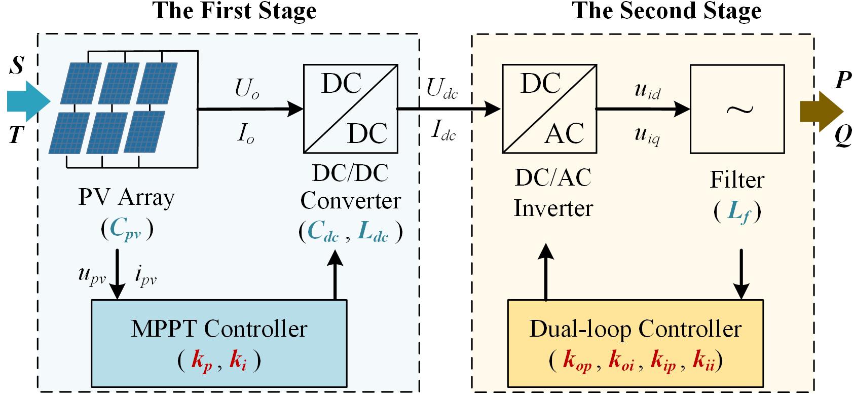
Figure 1. The structure of the two-stage PV station.
The First Stage Modeling of PV Station
In the First stage, the PV array converts the solar irradiance S into the electric energy, which is impacted by the ambient temperature T. Then, the DC-DC converter boosts the DC power by the array capacitance Cpv and control the PV array output voltage by the Maximum Power Point Tracking (MPPT) controller.
PV Array Modeling
The mathematic model of the PV array is essentially the single diode equivalent model (Hariharan et al., 2016). Its non-linear output characteristics are determined by four parameters, including open-circuit voltage, Uoc, short-circuit current, Isc, the maximum power voltage, Um, and the maximum power current, Im. The output characteristics of ipv - upv of the single PV module is described in Eq. (1). The coefficients C1 and C2 in (1) are determined by the values of Uoc, Isc, Um, and Im (Li P. et al., 2018).
Considering the series-parallel connection of the circuit, the output voltage Upv and current Ipv of the PV array can be formulated as (2) and (3) and the corresponding power output Ppv is presented in (4).
where Np and Ns are the parallel and series number of the modules in the PV, and the η is the conversion efficiency of the PV array.
DC-DC Converter Modeling
In Figure 1, the boost converter is selected as the DC-DC converter to maintain the current continuous (Chandra Mouli et al., 2017). The DC-DC boost converter and the PV array is connected by the array capacitance Cpv. The output characteristics of this connection in Laplace domain is given in Eq. (5).
where IL is the inductance current of the DC-DC boost converter.
The dynamic characteristics of the DC-DC boost converter can be represented as the switching cycle average model. When the capacitance Cdc and the inductance Ldc of the boost converter are enough large, the average output voltage Udc in the capacitance and the average output current Idc in the inductance in the Laplace domain are presented in Eqs (6) and (7).
where D is the duty ratio of the switch and determined by the MPPT controller.
MPPT Controller Modeling
The MPPT converter is used to control the switch status to guarantee the PV array output voltage can track the maximum voltage Um and work at the maximum power point (Dehedkar and Vitthalrao Murkute, 2018). The model of the controller in the Laplace domain is displayed as (8).
where kp and ki are the proportional gain and integral gain of the controller, respectively.
The Second Stage Modeling of PV Station
In the second stage, the DC-AC inverter converts the DC of PV output into three-phase AC with the same frequency and amplitude as the grid. The controller of the DC-AC inverter is a dual-loop controller including the DC voltage control and reactive power control. Besides, a filter is also needed for the harmonic suppression.
DC-AC Inverter Modeling
Power model of inverter is generally used in power flow calculation (Dutta and Chatterjee, 2018). The control strategy for inverter in this paper is SPWM control. Under SPWM mode, the output voltage of the inverter in d-q coordinate system is shown in (9).
where uid and uiq are components of the inverter output voltage in d-axis and q-axis, respectively, urd and urq are the components of the modulation wave voltage in d-axis and q-axis, respectively, and the Up is the peak voltage of the carrier wave.
Dual-Loop Controller Modeling
The control system is divided into inner loop control and outer loop control. The outer loop control consists of DC voltage outer loop control and reactive power outer loop control. The inner loop control is the current inner loop control.
In the outer loop control, the output voltage and current of PV array first determine the DC reference voltage Uref. Then, the difference between the actual measured voltage Udc and Uref is calculated. The reference current id,ref in the d-axis in the DC voltage outer loop control is presented in (10).
where kop and koi are the proportional and integral gains of outer loop control, respectively, and id is the d-axis component of the actual output current of the PV system.
The reactive power outer loop control compares the reactive power Qfilt measured from the filter circuit with the reference reactive power Qref to get the reactive power difference. The reference current iq,ref in q-axis is calculated by (11). The iq is the q-axis components of the actual output current of the PV system.
In the current inner loop, the SPWM modulation wave is generated, which is controlled by id,ref and iq,ref. The components of the SPWM modulation wave voltage in d-axis and q-axis, urd and urq, are shown as (12) and (13).
where kip and kii are the proportional and integral gains of inner loop control, respectively, usd and usq are the components of the actual grid voltage in q-axis and d-axis, the Lf is the filter inductance and ω is the angle frequency of the power grid.
Based on the description of the two-staged PV station modeling, the main factors affecting the output dynamic characteristics of PV station generation can be divided into physical and control parameters. The physical parameters contain the Cpv, Cdc, Ldc, and Lf. The control parameters consist of the control parameters of the MPPT controller and dual-loop controller, including kp, ki, kip, kii, kop, and koi. When the physic and control parameters are fixed, the corresponding output dynamic characteristics of the single PV station under the standard test condition is determined. Thus, the dynamic process f(⋅) of the single PV station can be described as (14).
The Framework of Data-Driven Hybrid Equivalent Dynamic Model for Central and Distributed PV Stations
Through the precise model of the dynamic characteristics of the single PV station in section “Precise Dynamic Modeling for A Single Two-Staged PV Station,” it is clear that the PV stations are highly non-linear system. With the penetration rate of the renewable energy increasing, the distributed PV stations gradually become the mainstream way, especially in industrial and rural areas. It brings in lots of uncertainty and stochastic for the power grid and makes the whole grid system quiet complex. Thus, it is necessary to build a dynamic equivalence model with high precision and short simulation time to study the impact of the central PV and large distributed PV stations. In Figure 2, a data-driven hybrid equivalent dynamic modeling approach is proposed. It consists of the physical equivalent model and error correction model.

Figure 2. The framework of data-driven hybrid equivalent dynamic modeling.
In the equivalent modeling part, the precise dynamic model of the PV stations is first simplified into the equivalent model from the aspect of physics, including the physical parameters equivalence and control parameters. According to the mathematical model of PV system in section “Precise Dynamic Modeling for A Single Two-staged PV Station,” physical parameters are composed of PV array capacitance Cpv, boost converter capacitance Cdc, boost converter inductance Ldc and filter inductance Lf. The control parameters include the control parameters of PWM system (kp, ki) and SPWM system (kip, kii, kop, koi). Since the distributed PV stations are installed in the different places and different feeders, the feeder equivalence is necessary for the distributed PV stations.
In the error correction modeling part, the errors between the physical equivalent and precise model are considered and corrected, including the steady-state error and the transient error. The steady-state error is usually small or a constant. The transient error is introduced by the equivalent control parameters and performs different in different test conditions. The data-driven approach is utilized to learn the errors of the dynamic output characteristics of the two models under multiple different work situations to make the hybrid equivalent model more accurate.
Equivalent Model for Central and Distributed PV Stations
The principle of simplifying an equivalent model of central PV stations and distributed PV stations is the output voltage and power of the equivalent model must be the same as the precise one. In addition, the distributed PV model are located at different places of different feeders. Thus, the node voltage and load need to be considered, while simplifying the distributed PV stations.
The Feeder Equivalence
Since distributed PV stations scatter in the feeders, one or more loads might exist between two PV stations. When multiple distributed PV stations are equivalent to a cluster in the system, the power distribution is also affected. Therefore, the node voltage and power flow should be considered while simplifying the distributed PV stations (Zhang et al., 2019). The load transfer and line impedance equivalence are implied on every node. The schematic diagram of feeder equivalence is displayed in Figure 3.
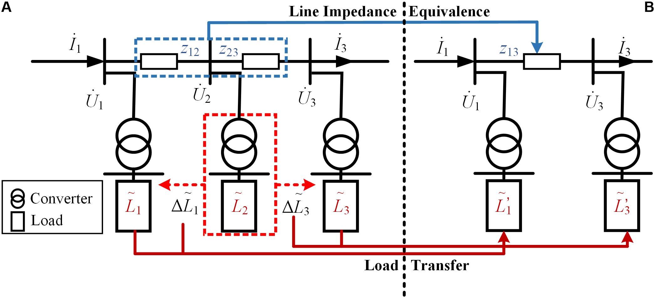
Figure 3. Schematic diagram of feeder equivalence. (A) Original feeder (B) equivalent feeder.
Suppose the voltage, injection current and load of the i-th node are denoted as , and , respectively. The impedance of line i-j is represented as zij. In Figure 3A, based on the Kichhoff’s current law, the relationship between the node 1 and node 3 can be presented as (15).
When node 2 disappears, the load of the node 2 is transferred into node 1 and node 3. The transfer amount of load from node 2 to node 1 and node 3 are denoted as and , respectively. Since the injection current of node 1 should keep equal to the output current of node 3 and the total power should remain unchanged, the values of and are calculated as (16) and (17). The load of node 1 and node 3 after the load transferring are and , presented in (18).
Except the load transfer of the node 2, the line impedance is also need to be modified, which impacts the line power loss. To keep the line power loss between node 1 and node 3 the same before and after the load transferring, the equivalent value of line impedance between node 1 and node 3 is displaye in (19).
After load transfer and feeder equivalence for each node in the network, multiple distributed PV stations can be equivalent to a single PV station model.
The Parameter Equivalence
In the parameter equivalence, it includes the physical parameters equivalence and control parameters adjustment. The principle of the physical parameters equivalence is based on the ratio of the total installed capacity of multiple PV stations to the installed capacity of a single PV station. Suppose n PV stations are clustered into one PV stations. The physical parameters of the i-th PV station, i = 1,2, …, n, include the capacitance and inductance parameters of the array, Cpv,i and Lpv,i, the capacitance and inductance parameters of the boost converter, Cdc,i and Ldc,i, and the inductance of filter, Lf,i. The corresponding aggregation parameters are determined by (20)–(22).
where the subscript EQ represents the equivalent value in the equivalent model and the value of the ρi is the ratio of the total installed capacity of n PV stations to the installed capacity of the i-th one.
Besides, considering each PV station connects to the power grid by a transformer, the capacity and impedance parameters of the transformer is also needed to be modified. The corresponding aggregation parameters are shown as (23).
where St,i and Zt,i are denoted as the rated capacity and impedance of the i-th PV station transformer.
The control parameters of the MPPT and dual-loop controller are adjusted after the aggregation physical parameters fixed. The initial control parameters in the equivalent model are determined by the average values of the control parameters of all the equivalent PV stations. To make the dynamic performance of the equivalent model close to the precise one, the control parameters are further adjusted artificially.
Ensemble GRU Based Error Correction Model
The distribution and aggregation of central PV stations and distributed PV stations are quite different. The physical and control parameters of each PV station in central PV plants are roughly equal, and their dynamic characteristics are close. But parameters of distributed PV stations are different. When the external conditions change, an obvious gap exists in their dynamic response. Thus, it is a data-driven error correction model is proposed in this section to fit the error between the precise model and the equivalent model. Considering the error data are the time series data, the GRU algorithm, which is powerful for dealing with the time series data, is used for modeling the errors.
At specific time t, the active power and reactive power of the equivalent model are denoted as EP(t) and EQ(t), respectively. The parameters, EP(t), EQ(t) and solar irradiance S are regarded as the input data of the error correction model. The target data of the error correction model are the corresponding errors of the active and reactive power at time t, CP(t) and CQ(t), which can be obtained by the precise and equivalent models.
The equivalent model and the accurate model are simulated under different conditions and a large amount of errors data are generated. The error dataset is then used to train the GRU to build the error correction model. The structural unit of GRU is shown in the Figure 4.
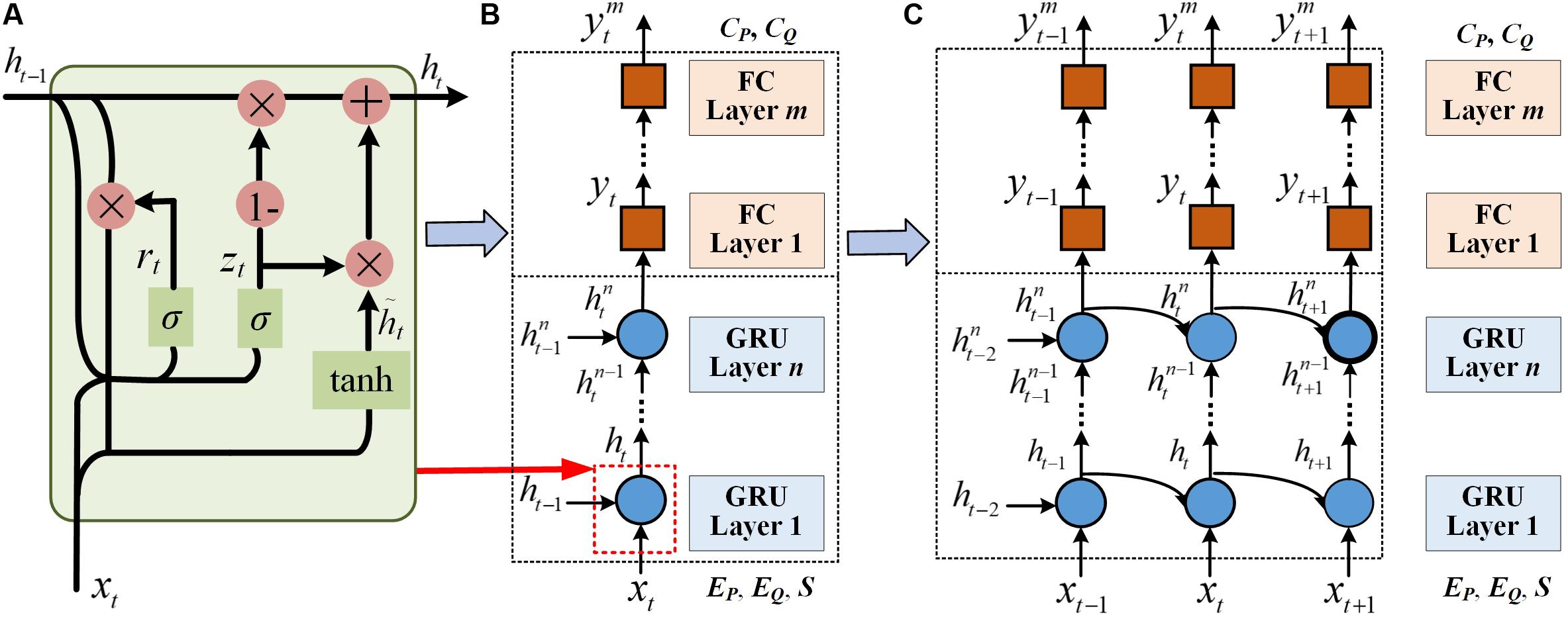
Figure 4. The structure of a single GRU model: (A) The structure of GRU layer, (B) The structure at a specific time t, (C) The structure for time series.
The Figure 4A displays the structure of the single GRU layer. The input data of each layer consists of the current error data xt and the hidden node ht–1 of the upper layer, where ht–1 contains the relevant information of the previous node. GRU contains two gates, a reset gate and an update gate. The parameter rt in the reset gate is used to control the degree of information forgetting in the previous moment. The parameter zt in the update gate is used to control the amount of information retained from time t-1 to t. After the gate processing, the data from the reset and update gates are added to get the data ht of the current layer. To enhance the information learning capacity, a single GRU base model is composed of n GRU layers, shown as Figure 4B. The Figure 4C shows the unfolded form of GRU model as the increasing of time t.
To further improve the accuracy and reduce stochastic of the neural network training, the ensemble technique is applied. In Figure 1, the structure of the ensemble GRU model is displayed. The BP neural network is used as the ensemble structure to train the weights of each sub-model. The whole dataset is divided into three parts, training dataset, validation dataset and test dataset.
The training dataset is firstly used to train the several GRU models, which are regarded as the sub-models of the ensemble model. To avoid the over-fitting phenomenon of the ensemble model, the data used to train each GRU are randomly selected through the bootstrapping technique. The structure of each GRU, such as the number of the units in each GRU layer, is also randomly generated.
Then, the outputs of each GRU model are regarded as the input of the BP neural network. The CP(t) and CQ(t) are regarded as the output. The weights of sub-models are learned by the validation dataset. At last, the testing data are used to verify the performance of the ensemble GRU model.
In the training process of the ensemble model, the data of EP(t), EQ(t) and S are first used as the input of each GRU model. The estimated active and reactive power errors of N GRU models are obtained, C’P, i(t) and C’Q, i(t), i = 1,…, N. To ensemble all the GRU models, the C’P, i(t) and C’Q, i(t) are regarded as the input of the BP neural network to the weights of each GRU. The active and inactive power estimated by the BP neural network are denoted as C’P(t) and C’Q(t). The active and reactive power of the hybrid model at time t, P’(t) and Q’(t), are calculated through (24) and (25).
Case Study
In this section, the proposed method is validated through a radial active distributed network simulation system, shown in Figure 5A. In Figure 5A, there are a central PV stations and 8 distributed PV stations (PV1∼PV8). Since the central PV station has two different types of PV, it is divided into two parts, central PV station 1 and central PV station 2. In addition, the PV system includes transformers, transmission lines and loads. The installed capacities of the 10 two-staged PV stations are: 21 kW for PV1 and PV2, 23.4 kW for PV3 and PV4, 18 kW for PV5 and PV6, 18.6 kW for PV7 and PV8,475 kW for central PV station 1 and 338 kW for central PV station 2. The total installed capacity is 975 kW and the total load is 1532+j781kVA. The parameters of PV system are set according to the PV system used in engineering. The sample frequency is set to 500 Hz. Since the system reaches the steady state after 0.25 s, the sample time period is set from 0.25 to 0.55 s. Each group contains 150 sampling points.
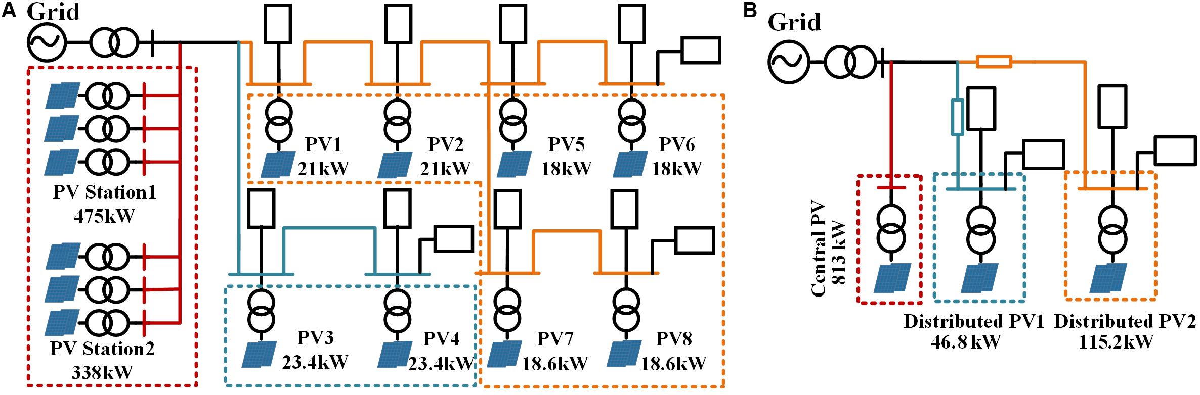
Figure 5. Schematic diagram of the multiple PV stations system: (A) The original system, (B) The equivalent system.
The detailing physical and equivalent physical system are built on the Simulink platform in Matlab. The first stage of the model is composed of the PV array, converter, MPPT controller and PWM controller. The first stage calls the PI controller model, integrator model, saturation model, product model and other mathematical models in Simulink Library. PI controller model and saturation model are used to realize PWM control. MPPT controller is affected by PWM controller and consists of mathematical models. The second stage is composed of the inverter, filter and dual-loop controller. Compared with the first stage, the second stage calls the vector conversion model in Simulink Library additionally. The vector conversion model converts three-phase current into d-q coordinate system.
The error correction model is built by Keras on the Pycharm platform. The simulations are conducted on a PC with Intel (R) CPU i7-6500U, 2.5 GHz, RAM 8 GB.
Experiment Settings
The Settings of PV Stations and Test Scenarios
The physical and control parameters of each PV stations, which determines their dynamic process performance are shown as Table 1. In Table 1, it is obvious the control parameters of each PV station are quite different, which brings lots of difficulties on the control parameter setting of the equivalent model. The error correction model can make up the difference between the precise model and equivalent model. Thus, the requirement of the equivalent model is reduced by building the error correction model.
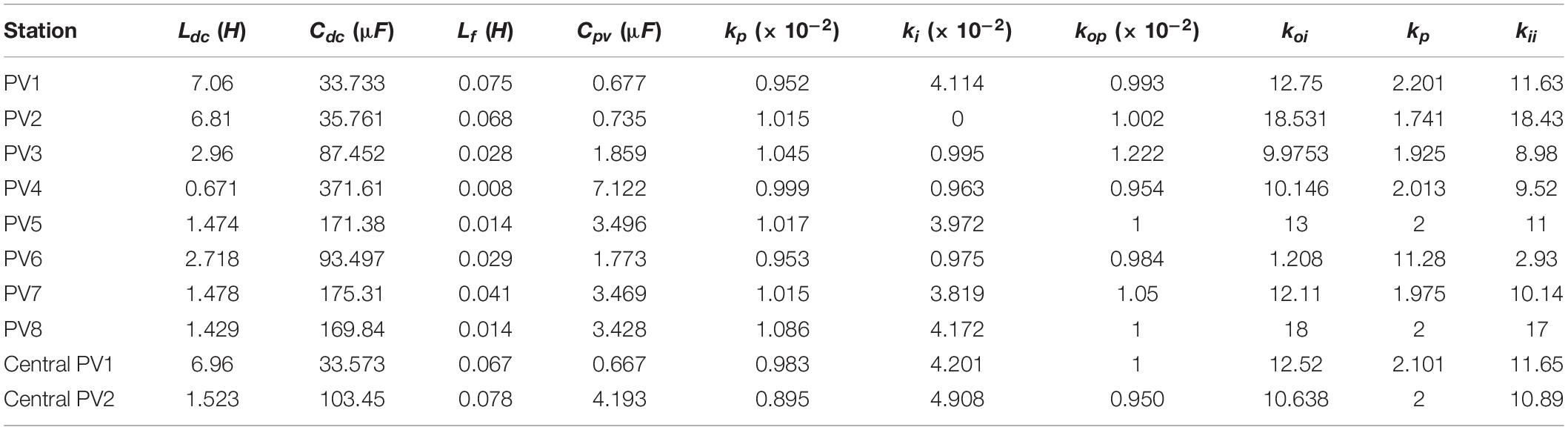
Table 1. Physical and control parameters of PV stations.
In order to validate the universality of the model, three test scenarios are designed. In Case I, the random disturbance is considered and added into the input irradiance data, which can be described as the random input signal. This case represents the shift of the day and night and the situation of load slightly reducing and increasing. In Case II and Case III, the abrupt change of the input irradiance data is considered. In Case II, the rapid rise or fall of irradiance appears in a short period of time and remains stable, which can be called as the step input signal. This case is used to describe the instantaneous change in irradiance, the situation of short circuit or instantaneous load rejection. In Case III, a continuous and rapid rise and fall of the irradiance happens over a very short period of time, named as pulse input signal.
To train a general error correction model, the data under different test scenarios are needed to be collected. The detailed settings of three cases for data collection are shown as follows:
Case I: set the irradiance from 300 to 1500 W/m2, and noise is set from 5 to 40 W/m2. This case has 960 groups of experiments.
Case II: set the irradiance from 300 to 1500 W/m2. The abrupt change happens at 0.33 s and the change amplitude is set from 40 to 120 W/m2. This case has 960 groups of experiments.
Case III: set the irradiance from 300 to 1500 W/m2. The abrupt changes happen at 0.27 and 0.37 s. The change amplitude is set from 40 to 120 W W/m2. This case has 960 groups of experiments.
The Settings of Ensemble GRU
Since the active power is greatly impacted by the external factors, the ensemble model of active power contains 50 GRU base models. Since the variance of the reactive power is relatively stable, the ensemble model is set to include 25 base models. Each GRU base model has the same number of the hidden layers, including 3 GRU layers and 3 full connection (FC) layers. The activation function of the GRU layer is tanh function and the FC layer is Relu function. To reduce the impact of the over-fitting, the dropout layer is added after the first and second GRU layers. The number of units of the different GRU layers are randomly generated to form different GRU base models. The detailed parameter setting of a single GRU base model is shown as Table 2. The Adam optimizer is used to train the GRU base model. 150 samples are randomly selected as a batch.
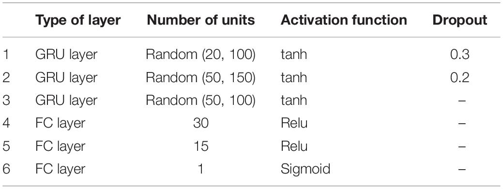
Table 2. Parameter setting of a single GRU based model.
To avoid the neuron saturation, the sample data of every moment is normalized by the min-max normalization, which maps each sample data to [0, 1], shown as (26).
where X is the actual value of input variable, Xmin and Xmax are the minimal and maximal value of input variable, and X’ is the corresponding normalized value. The sequences of collected 3000 groups are disordered. The 2000 groups of samples are used to form the training dataset and the rest groups for testing. The root mean square error (RMSE) is used to evaluate the performance of the error correction model. The RMSE of each group is shown as (27).
where Ct is the output of error correction model, Et is the actual error, t is the index of the time step in each group, and N is the total number of samples in each group. The RMSE of training dataset and test dataset are calculated by average the RMSEs of all groups in the dataset.
Simulation Performance and Analysis
Simulation Result
In this section, the performance of the data-driven hybrid model is displayed and analyzed under the three test scenarios. According to the above equivalent method, the equivalent model of PV system is first established. The central PV1 and central PV2 are equivalent to a PV station with the capacity of 813 kW. Then, all the distributed PV stations located in the same branch are equivalent to one PV station. The distributed PV stations are equivalent as two PV stations, distributed PV1 and PV2 according to the distribution characteristics. The equivalent model of the system is displayed as Figure 5B. The corresponding equivalent parameters of equivalent PV stations are given in Table 3.
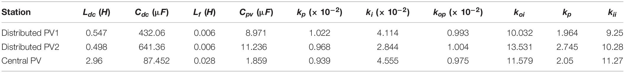
Table 3. Physical and control parameters of equivalent models.
Table 4 shows the RMSE between three equivalent models and the precise model. The hybrid model is the data-driven hybrid equivalent model with single GRU. The hybrid ensemble model is the data-driven hybrid equivalent with ensemble GRU. In Table 4, it is clear that RMSE is significantly reduced after introducing error correction model. The error of model with ensemble GRU is smaller than the one with single GRU for all three scenarios. Since the impact of the reactive power affected by the changes of irradiance and load is less than the active power, the error correction model performs better for the reactive power. In Case I, the irradiance fluctuates slightly and the errors are the least among three scenarios. The Case III has two rapid disturbances and the greater errors than Case I and Case II.
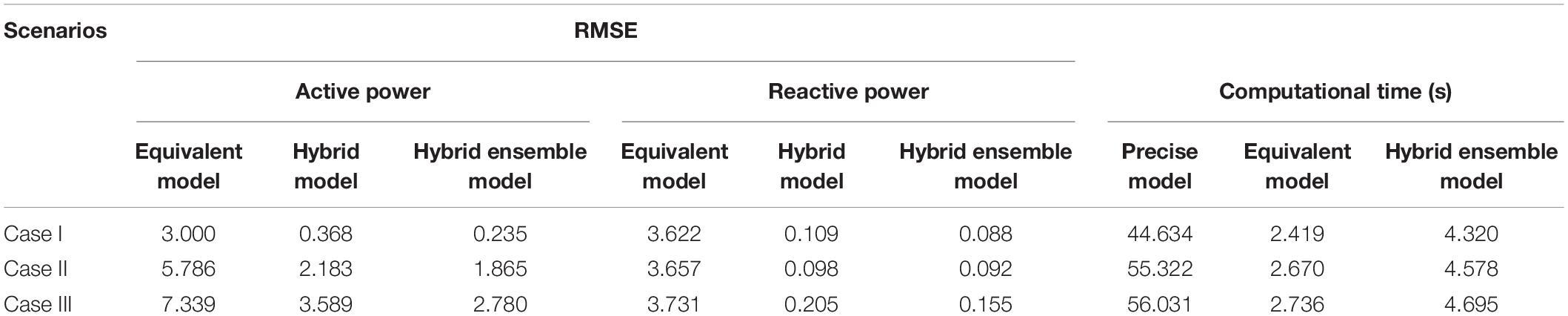
Table 4. Computational errors (RMSE) and computational time of different models.
Table 4 also shows the simulation time required for the precise model, equivalent model and data-driven hybrid ensemble model. It can be seen that the simulation time of the hybrid model with ensemble GRU is far less than that of the precise model. The error correction model needs the active and reactive power time-series output of the equivalent model and work after the equivalent. Besides, the error correction model contains multiple GRU models, which needs the time to obtain output of each GRU model. Combined with the above two points, the simulation time of the hybrid ensemble model is longer than that of the equivalent model. This advantage becomes more and more obvious with the complexity of system increasing. The purpose of reducing simulation time is realized by using the data-driven hybrid model.
Besides, Figure 6 shows the training and test results of active power by ensemble GRU under Case II, respectively. The result of test dataset is close to that of training dataset, which indicates that there is no over fitting or under fitting.
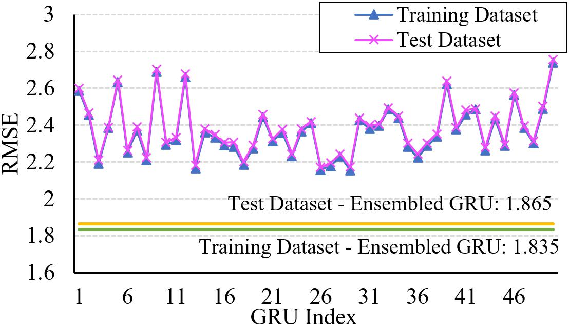
Figure 6. RMSE of active power of each GRU base model and ensemble GRU model in Case II.
Simulation Example Under Different Test Scenarios
In Figure 7, three test examples are separately selected from three test scenarios. In Figure 7A, the irradiance randomly changes from 830 to 850 W/m2. The irradiance randomly changes within a small margin. In this situation, the PV system usually works in a disturbed environment which means it is always in a dynamic process. The active and reactive power response of different models in this case are shown in Figure 8. It is obvious that there is a certain error between the equivalent and precise models. After the introducing error correction model, the error between the power output of the equivalent and precise model is significantly reduced. Besides, the reactive power is less impacted by the change of the random irradiance and keeps stable in the whole process.
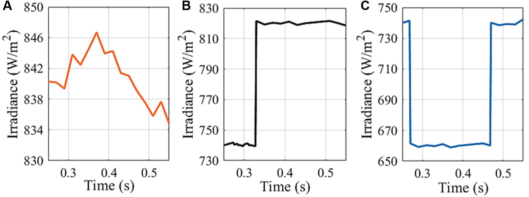
Figure 7. Examples of irradiance input data in three test scenarios: (A) Case I, (B) Case II, (C) Case III.
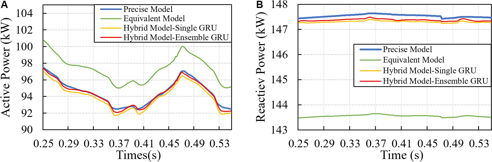
Figure 8. Example of the response of precise, equivalent and hybrid model in Case I: (A) Active power, (B) Reactive power.
In the example of Case II, the irradiance rapidly rises from 740 to 820 W/m2, shown as Figure 7B. This scenario can reflect the operation of load rejection and load increase in the infinite source power grid. The load change in the power grid is usually long-term and completed in a short time, which can be approximated as the step response. Figure 9 gives the corresponding active and reactive power response. When irradiance rapidly rises or falls in a short period of time, the dynamic characteristics of the equivalent model approach to the oscillation process. After using single GRU model for error tracking, the output characteristics of the equivalent model are improved to some extent, but there are still some deviations. The error tracking of Ensemble GRU model is further improved. The raised errors in some areas are eliminates through Ensemble GRU, such as the error appearing from 0.39 to 0.44 s.
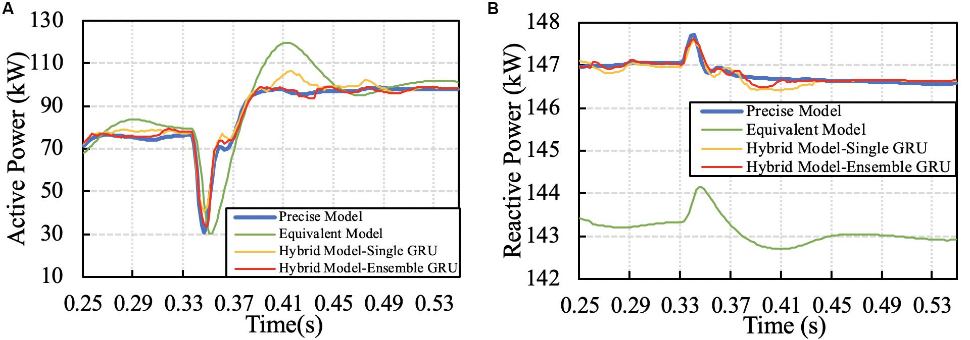
Figure 9. Example of the response of precise, equivalent and hybrid model in Case II: (A) Active power, (B) Reactive power.
In Case III, the irradiance rapidly falls from 740 to 660 W/m2 at 0.27 s and then rises to 740 W/m2 at 0.37 s, shown as Figure 7C. This scenario reflects the instantaneous disturbance of PV system and can represent that the PV system is blocked for a short time or the grid is short-circuited. The corresponding active and reactive power response are shaped in Figure 10. In this case, due to the short time interval between two abrupt disturbs, the influence of control parameters is amplified. It is clear that the dynamic response of the equivalent model is slower than the precise one. Through the error correction, this lag is almost removed. Under this condition, the hybrid model can still track the error accurately.
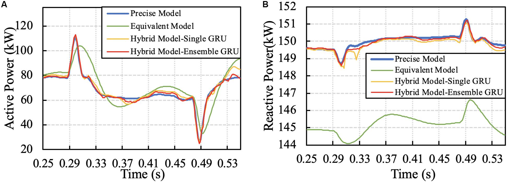
Figure 10. Example of the response of precise, equivalent and hybrid model in Case III: (A) Active power, (B) Reactive power.
Conclusion
This paper proposed a hybrid data-driven model to build the equivalent model of the dynamic process of the multiple PV stations in the distributed network. The dynamic process of the PV system were described by the physical and control parameters. The data model and the physical model were combined to build an accurate model.
The equivalent models for central and distributed PV stations were firstly established from the physical aspect. The equivalent models needed to consider the physical parameter and feeder equivalence. Since the control parameters were determined artificially, the errors existed between the simple equivalent model and the precise model. The data-driven model was introduced to track and correct the errors.
The ensemble GRU model was utilized as the error correction model. Three different test cases were established to help build the error correction model of the active and reactive power. The simulation results showed that the proposed hybrid data-driven model improved the fitting precision of the dynamic characteristics while keeping the low model complexity and short computational time.
Data Availability Statement
The raw data supporting the conclusions of this article will be made available by the authors, without undue reservation, to any qualified researcher.
Author Contributions
HL: conceptualization, methodology, and writing – reviewing and editing. SX: data curation, software, and writing – original draft preparation. All authors contributed to the article and approved the submitted version.
Funding
This article was supported with the Science and Technology Program of State Grid Corporation of Jiangsu Province: Research and Application of Integrated Energy Regulation Technology Aiming at the Interaction of Source, Grid, Load, and Storage (Grant No. 521002190049), and the National Natural Science Foundation of China under Grant 51807023.
Conflict of Interest
XL, ZY, and JJ were employed by company State Grid Jiangsu Electric Power Company Limited. CL was employed by company National Electric Power Dispatching and Communication Center.
The remaining authors declare that the research was conducted in the absence of any commercial or financial relationships that could be construed as a potential conflict of interest.
References
Abido, M. A., and Sheraz Khalid, M. (2018). Seven-parameter PV model estimation using differential evolution. Electr. Eng. 100, 971–981. doi: 10.1007/s00202-017-0542-2
Batzelis, E. I. (2017). Simple PV performance equations theoretically well founded on the single-diode model. IEEE J. Photovolt. 7, 1400–1409. doi: 10.1109/JPHOTOV.2017.2711431
Chandra Mouli, G., Schijffelen, J., Bauer, P., and Zeman, M. (2017). Design and comparison of a 10-kW interleaved boost converter for PV application using Si and SiC devices. IEEE J. Emerg. Select. Top. Power Electron. 5, 610–623. doi: 10.1109/JESTPE.2016.2601165
Dehedkar, M., and Vitthalrao Murkute, S. (2018). “Optimization of PV system using distributed MPPT control,” in Proceedings of the 2018 International Conference on System Modeling & Advancement in Research Trends (SMART), (Moradabad: IEEE).
Dutta, S., and Chatterjee, K. (2018). A buck and boost based grid connected PV inverter maximizing power yield from two PV arrays in mismatched environmental conditions. IEEE Trans. Ind. Electr. 65, 5561–5571. doi: 10.1109/TIE.2017.2774768
Ferreira, A., Kunh, S. S., Fagnani, K. C., De Souza, T. A., Tonezer, C., Dos Santos, G. R., et al. (2018). Economic overview of the use and production of photovoltaic solar energy in brazil. Renew. Sustain. Energy Rev. 81, 181–191. doi: 10.1016/j.rser.2017.06.102
Hariharan, R., Chakkarapani, M., Saravana Ilango, G., and Nagamani, C. (2016). A method to detect photovoltaic array faults and partial shading in PV systems. IEEE J. Photovolt. 6, 1278–1285. doi: 10.1109/JPHOTOV.2016.2581478
Kim, J., Kwon, J., and Kwon, B. (2018). High-efficiency two-stage three-level grid-connected photovoltaic inverter. IEEE Trans. Indust. Electr. 65, 2368–2377. doi: 10.1109/TIE.2017.2740835
Li, P., Gu, W., Long, H., Cao, G., Cao, Z., Xu, B., et al. (2019). High-precision dynamic modeling of two-staged photovoltaic power station clusters. IEEE Trans. Power Syst. 34, 4393–4407. doi: 10.1109/TPWRS.2019.2915283
Li, P., Gu, W., Wang, L., Xu, B., Wu, M., and Shen, W. (2018). Dynamic equivalent modeling of two-staged photovoltaic power station clusters based on dynamic affinity propagation clustering algorithm. Int. J. Electr. Power Energy Syst. 95, 463–475. doi: 10.1016/j.ijepes.2017.08.038
Li, W., Chao, P., Liang, X., Ma, J., Xu, D., and Jin, X. (2018). A practical equivalent method for DFIG wind farms. IEEE Trans. Sustain. Energy 9, 610–620. doi: 10.1109/TSTE.2017.2749761
Muhammad Qamar, R., Nadarajah, M., and Ekanayake, C. (2016). On recent advances in PV output power forecast. Solar Energy 136, 125–144. doi: 10.1016/j.solener.2016.06.073
Piazza, M., Luna, M., Petrone, G., and Spagnuolo, G. (2017). Translation of the single-diode PV model parameters identified by using explicit formulas. IEEE J. Photovolt. 7, 1009–1016. doi: 10.1109/JPHOTOV.2017.2699321
Remon, D., Cantarellas, M., and Rodriguez, P. (2016). Equivalent model of large-scale synchronous photovoltaic power plants. IEEE Trans. Ind. Appl. 52, 5029–5040. doi: 10.1109/TIA.2016.2598718
Sangwongwanich, A., Yang, Y., and Blaabjerg, F. (2017). A sensorless power reserve control strategy for two-stage grid-connected PV systems. IEEE Trans. Power Electron. 32, 8559–8569. doi: 10.1109/TPEL.2017.2648890
Shao, C., Wang, W., Hang, L., Tong, A., and Wang, S. (2018). “A novel PV array connection strategy with PV-buck module to improve system efficiency,” in Proceedings of the 2018 International Power Electronics Conference (IPEC-Niigata 2018 -ECCE Asia), (Niigata: IEEE).
Siouane, S., Jovanoviæ, S., and Poure, P. (2019). Open-switch fault-tolerant operation of a two-stage buck/buck–boost converter with redundant synchronous switch for PV systems. IEEE Trans. Ind. Electron. 66, 3938–3947. doi: 10.1109/TIE.2018.2847653
Xiang, J., Wei, W., and Cai, H. (2016). Modelling, analysis and control design of a two-stage photovoltaic generation system. IET Renew. Power Gener. 10, 1195–1203. doi: 10.1049/iet-rpg.2015.0514
Yamaguchi, D., and Fujita, H. (2018). A new PV converter for a high-leg delta transformer using cooperative control of boost converters and inverters. IEEE Trans. Power Electron. 33, 9542–9550. doi: 10.1109/TPEL.2018.2791343
Zapata, J., Kouro, S., Carrasco, G., Renaudineau, H., and Meynard, A. T. (2019). Analysis of partial power DC–DC converters for two-stage photovoltaic systems. IEEE J. Emerg. Select. Top. Power Electron. 7, 591–603. doi: 10.1109/JESTPE.2018.2842638
Zhang, M., Song, B., and Wang, J. (2019). Circulating current control strategy based on equivalent feeder for parallel inverters in islanded microgrid. IEEE Trans. Power Syst. 34, 595–605. doi: 10.1109/TPWRS.2018.2867588
Keywords: central PV power station, distributed PV power station, data-driven dynamic modeling, equivalent model, gated recurrent unit
Citation: Long H, Xu S, Lu X, Yang Z, Li C, Jing J and Wu Z (2020) Data-Driven Hybrid Equivalent Dynamic Modeling of Multiple Photovoltaic Power Stations Based on Ensemble Gated Recurrent Unit. Front. Energy Res. 8:185. doi: 10.3389/fenrg.2020.00185
Received: 27 May 2020; Accepted: 14 July 2020;
Published: 31 July 2020.
Edited by:
Long Wang, University of Science and Technology Beijing, ChinaReviewed by:
Shancheng Jiang, Sun Yat-sen University, ChinaWei Liu, Nanjing University of Science and Technology, China
Copyright © 2020 Long, Xu, Lu, Yang, Li, Jing and Wu. This is an open-access article distributed under the terms of the Creative Commons Attribution License (CC BY). The use, distribution or reproduction in other forums is permitted, provided the original author(s) and the copyright owner(s) are credited and that the original publication in this journal is cited, in accordance with accepted academic practice. No use, distribution or reproduction is permitted which does not comply with these terms.
*Correspondence: Huan Long, hlong@seu.edu.cn