A Novel Geometric Error Compensation Method for Gantry-Moving CNC Machine Regarding Dominant Errors

Abstract

Gantry-type computer numerical control (CNC) machines are widely used in the manufacturing industry. A novel structure with moveable gantry is proposed to improve the traditional gantry-type machine structure’s disadvantage of taking up too much space. Geometric errors have direct impacts on the actual position of the tool, which significantly reduces the accuracy of machines. Errors of different components are always coupled and have uncertain effects on the total geometric error. Thus, it is essential to find an effective way to identify the dominant errors and do targeted compensation. First, a novel identification method using value leaded global sensitivity analysis (VLGSA) is proposed to find the dominant errors. In VLGSA, weighting factors which show the influence of the error range are used to modify the multi-body system (MBS) error model. Results show that the dominant errors in three directions respectively contribute 80%, 86% and 85% of the total error in their directions. Then, errors identified by VLGSA are modeled by least-square linear fitting and B-spline interpolation methods, respectively, according to the feature of error data. Finally, the models are applied in a new real-time compensation system developed on the Beckhoff TwinCAT servo system. Experimental results from the gantry-type CNC engraving and milling machine show the proposed method can help figure out the most dominant errors and reduce around 90% of the total error.

1. Introduction

Gantry-type manufacturing equipment has already played an indispensable role in the modern manufacturing industry. In traditional gantry-type machines, the X-direction feed movement is realized by the motion of workbench, while the gantry is fixed on the machine bed. A vast room of more than twice the feed stroke should be reserved to ensure the processing capability, which causes the waste of space. Thus, a novel structure with a moveable gantry is proposed. Different from the traditional structure, the workbench is fixed and two ball-screw feed systems are symmetrically arranged to drive the gantry. Only half the space is needed comparing with the traditional one. However, machines with moveable gantries require higher accuracy. Many factors are affecting the accuracy of gantry-type machine tools, such as geometric error, thermal error, servo system error and so forth. Thermal errors widely appear in engineering machinery devices and many researchers have done great jobs on optimizing heat transformation [1,2,3,4]. Geometric error is another common component and usually donates most in the final inaccuracy [5]. The geometric errors directly influence the final position of the tool nose and the errors are generally related to the tiny defect of the machine itself, like the wrong structure of the feed system. There are two ways to resolve the problem. One is adjusting the physical structure, which is complicated and expensive and may be limited by the skill of the technical staff. The other one is compensating for the existing errors by numerical control (NC) code or software, which is much more flexible and can achieve high quality [6]. However, the compensation needs a clear understanding of the existing errors. Error modeling is firstly required to reach the goal.

The technique of geometric modeling has been persistently developed in recent decades. In the application of the robot industry, Paul, R.P. [7] and Veitschegger, W.K. [8] gave methods using the homogeneous transformation matrix and differential transformation. The precise location of the robot’s terminal point with the existence of geometric size errors and kinematic errors was found in their research. These works established the basis of error analysis. Chen, J.X. et al. [5] took further research based on the fundamental principle of Paul and Veitschegger, by analyzing the differential movement and differential transformation. They proposed a comprehensive method of both discovering how geometric error propagates through every single axis. Zhao, Q.Q. et al. [9] established the topology structure of the machine tool using multi-body system theory and proposed two conceptions, which were relative motion matrices of axis and connectors and connection matrix of machine tool connectors. Based on the homogeneous coordinate transformation theory, Zhou, X.T. [10] built the error model of the classic three-axis machine tool, decomposed the final error into the errors existing in the components in the whole motion chain. These works showed the development and application of different error modeling methods, gave inspirations to further research. Still, many of them were limited in modeling. Models based on these methods are usually complex mathematical expressions of a vast amount of error items, making it a sophisticated work to compensate for all the items. However, compensation towards several specific error items, which can be defined as dominant errors, may provide enough accuracy improvement. Thus, more research could be done to simplify the compensation.

Sensitivity analysis (SA) is a kind of method to quantify the uncertainties of an unknown system using great data, which may help in finding the most valuable error items to compensate. For a specific model, a vast amount of different input and output data can be obtained through all kinds of scientific sampling methods and powerful calculation tools. Thus the sensitivity analysis can help to identify the weight each input has in affecting system outputs. SA consists of two main branches, one is local sensitivity analysis (LSA) and the other is called global sensitivity analysis (GSA). [11,12] The GSA is more commonly used in the manufacturing industry with its ability to find out the result differences under the changes of parameters. It can emphasize the interaction power of the parameters by using additional methods. Usually, SA is used in economic analysis. However, it is also found suitable in the engineering field recently.

Fan, J.W. et al. [13] established a prediction model of component tolerance and proposed a sensitivity analysis based on component motion. The proposed sensitivity analysis was experimentally verified and several main parameters that donate to errors most were found out. Yan, Y. et al. [14] established the error model of multi-process assembling and built the sensitivity analysis model of parameters towards assembling error using the method of matrix differentiation. Li, J. and Xue, F.G. [15] proposed general local sensitivity indices (GLSIs), general global sensitivity indices (GGSIs) and general global sensitivity fluctuation indices (GGSFIs) based on traditional sensitivity analysis. A five-axis machine was analyzed using the above indices. One common limit of the above works is that the sensitivity indices calculation is carried out on the original error model without considering the impact of error value range towards sensitivity analysis. Besides, sensitivity analysis of machine tools was only done for performance assessment, targeted compensation was missing and validity was not verified.

Sensitivity analysis tells what to concentrate on; error measurement and fitting tell how to describe and deal with them. With all kinds of advanced measurement equipment, precision error data can be obtained. According to the error data, the error model can be established for compensation. However, appropriate fitting methods are needed to ensure the compensation accuracy. To improve manufacturing performance, many researchers have done great works. Fang, K.G. and Yang, J.G. [16] considered thermal factors, used the orthogonal polynomial method to build the total error model, compensated 90% of spindle geometric error. Wang, W. et al. [17] used the Newton interpolation method to construct the thermal and geometric error model of the computer numerical control (CNC) milling machine, established a real-time compensation system. The experiment based on the Fanuc CNC machine was carried out to show the compensation system works well. Tuo, Z.Y. et al. [18] using cubic spline interpolation established the thermal and geometric error model and improved the position accuracy of the CNC machine. The B-spline curve is commonly used in computer aided design (CAD) areas for its ability to describe the continual material. It is also used in trajectory planning for its smooth character. Li, Y.H. et al. [19] used the quantic B-spline curve to optimize the motion path of pick-and-place robots. His work showed that the B-spline curve is appropriate for smooth machine motion, which is also suitable for compensation relative movement of machine tools.

In this paper, the multi-body system theory was used to establish the geometric error model of the gantry-moving engraving and milling machine. Then the translation errors in all three directions are extracted from the error matrix to analyze the significant error items which impact the precision most. Value leaded global sensitivity analysis (VLGSA) is proposed and used in the above analysis process, in which the measurement value of each error item is considered to modify the total geometric error model. The B-spline curve was developed into the B-spline interpolation method and used on the result of machine error measurement. A real-time compensation system based on the Beckhoff servo system, TwinCAT control software and C# language was built to eliminate the errors. The compensation experiment verified the validity of the above crucial error finding and compensation method.

2. Geometric Modeling Based on Multibody System

The multi-body system (MBS) illustrates a kind of mechanical system in which a series of rigid or flexible bodies interconnect [20]; every single body may undergo translation and rotation in different scales. It is a general and systematic method for geometric error modeling and is widely used in the analysis of robots, machine tools and coordinate measurement.

The core of MBS is using the low-order-body arrays to describe the topology structure of the system [20], using transformation matrices to calculate the motion relationship. Usually, the inertial coordinate system is chosen as body B₀, the basic component is selected as body B₁, other elements are divided into several branches and the numbered along the direction away from B₁, branch by branch.

2.1. Coordinate System Definition and Topology Structure Description of the Gantry-Moving CNC Machine

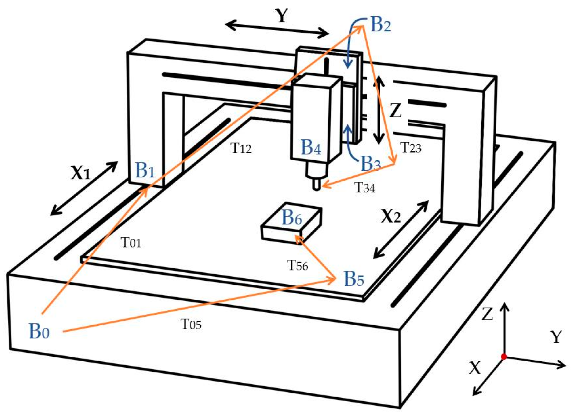
In this paper, a gantry-moving engraving and milling machine with three-dimension movements is taken to describe the ideal of presented geometric error modeling method. The structure of the chosen machine is shown in Figure 1.

The gantry-moving CNC machine has two servo motors in the X direction. Two motors are symmetrically arranged to drive the gantry through ball-screw feed systems. X1 and X2 represent the movement of two feed systems. The synchronization error between two movements is an important cause of X-direction yaw error.

Since the machine locates on a stable ground coordinate system, the machine bed itself can be directly chosen as body B₀. As the orange lines show in Figure 1, the engraving and mill machine can be seen as a two-branch topology structure [21]. The first branch (tool branch) consists of the moveable gantry (B₁), Y direction slide (B₂), Z direction slide (B₃) and the spindle with the tool on it (B₄). The second branch (workpiece branch) consists of the workbench (B₅) and the workpiece (B₆).

Table 1. Size of main components.

Main Parameters of the Components	Value (mm)
Size of the workbench (width × length)	3000 × 1500
Stroke of the gantry (X-direction stroke)	2400
Stroke of the Y slide (Y-direction stroke)	1200
Stroke of the Z slide (Z-direction stroke)	240

shows the main sizes of these components.

The final topology structure and coordinate definition with the position and motion relationships are shown in Figure 2, where the vectors between bodies show their relations. Take B₀ and B₁ as an example, T_01p means the position transformation between B₀ and B₁; T_01s means the motion transformation between B₀ and B₁; T_01pe and T_01se represent the error of position and motion transformations respectively. T_01p, T_01pe, T_01s and T_01se constitute the total coordinate transformation between B₀ and B₁ (T₀₁).

Table 2. Low-order-body Array of Chosen Machine.

Body	1	2	3	4	5	6
L1(j)	0	1	2	3	0	5
L2(j)		0	1	2		0
L3(j)			0	1
L4(j)				0

shows the low-order-body array of the machine, in which L is the low-order-body operator. For body B_j, its n-th order low-order-body number can be defined as Equation (1):

$${\mathrm{L}}^{\mathrm{n}}(\mathrm{j})=\mathrm{i}$$

(1)

where n means that B_i is the n-th order low-order-body of body B_j

Similarly, other equation can be inferred as Equations (2) and (3):

$${\mathrm{L}}^{\mathrm{n}}(\mathrm{j})=\mathrm{L}({\mathrm{L}}^{\mathrm{n}-1}(\mathrm{j}))$$

(2)

$${\mathrm{L}}^0(\mathrm{j})=\mathrm{j}.$$

(3)

2.2. Coordinate Transformation and Model Establishment

The actual position and motion between bodies can be expressed by matrix, more specifically by position matrix, motion matrix, position error matrix and motion error matrix. After binging every single body to their fixed coordinate, the position and motion transformation can be demonstrated by the multiplication of a series of 4 × 4 homogeneous eigenmatrix [22].

For a three-dimensional Cartesian coordinate system, translation can be expressed as Equation (4), in which x, y and z are translation along three axes, respectively. Rotation around three axes can be expressed as Equations (5)–(7).

$$\mathrm{T}=\left[\begin{array}{cccc}1& 0& 0& \mathrm{x}\\ 0& 1& 0& \mathrm{y}\\ 0& 0& 1& \mathrm{z}\\ 0& 0& 0& 1\end{array}\right]$$

(4)

$$\mathrm{R}\mathrm{o}\mathrm{t}(\mathrm{x},{\mathsf{\theta }}_{\mathrm{x}})=\left[\begin{array}{cccc}1& 0& 0& 0\\ 0& \mathrm{c}\mathrm{o}\mathrm{s}{\mathsf{\theta }}_{\mathrm{x}}& -\sin {\mathsf{\theta }}_{\mathrm{x}}& 0\\ 0& \sin {\mathsf{\theta }}_{\mathrm{x}}& \cos {\mathsf{\theta }}_{\mathrm{x}}& 0\\ 0& 0& 0& 1\end{array}\right]$$

(5)

$$\mathrm{R}\mathrm{o}\mathrm{t}(\mathrm{y},{\mathsf{\theta }}_{\mathrm{y}})=\left[\begin{array}{cccc}\cos {\mathsf{\theta }}_{\mathrm{y}}& 0& \sin {\mathsf{\theta }}_{\mathrm{y}}& 0\\ 0& 1& 0& 0\\ -\sin {\mathsf{\theta }}_{\mathrm{y}}& 0& \cos {\mathsf{\theta }}_{\mathrm{y}}& 0\\ 0& 0& 0& 1\end{array}\right]$$

(6)

$$\mathrm{R}\mathrm{o}\mathrm{t}(\mathrm{z},{\mathsf{\theta }}_{\mathrm{z}})=\left[\begin{array}{cccc}\cos {\mathsf{\theta }}_{\mathrm{z}}& -\sin {\mathsf{\theta }}_{\mathrm{z}}& 0& 0\\ \sin {\mathsf{\theta }}_{\mathrm{z}}& \cos {\mathsf{\theta }}_{\mathrm{z}}& 0& 0\\ 0& 0& 1& 0\\ 0& 0& 0& 1\end{array}\right]$$

(7)

However, both structure error and motion error exist in the manufacturing process. Take the X-direction movement as an example (shown in Figure 3). Errors between two coordinates can be divided into six types, including three linear error and three angle error. Linear errors are position error and straightness error along with two directions. Angle errors are roll error, pitch error and yaw error. Similarly, geometric errors in other directions can be defined as

Table 3. Geometric errors in the chosen caving and milling machine.

Error Type	Error Item	Error Symbol
X-direction feed errors	Position error	$\Delta {\mathrm{x}}_{\mathrm{x}}$
	Y-direction straightness error	$\Delta {\mathrm{y}}_{\mathrm{x}}$
	Z-direction straightness error	$\Delta {\mathrm{z}}_{\mathrm{x}}$
	Roll error	$\Delta {\mathsf{\alpha }}_{\mathrm{x}}$
	Pitch error	$\Delta {\mathsf{\beta }}_{\mathrm{x}}$
	Yaw error	$\Delta {\mathsf{\gamma }}_{\mathrm{x}}$
Y-direction feed errors	Position error	$\Delta {\mathrm{y}}_{\mathrm{y}}$
	X-direction straightness error	$\Delta {\mathrm{x}}_{\mathrm{y}}$
	Z-direction straightness error	$\Delta {\mathrm{z}}_{\mathrm{y}}$
	Roll error	$\Delta {\mathsf{\beta }}_{\mathrm{y}}$
	Pitch error	$\Delta {\mathsf{\alpha }}_{\mathrm{y}}$
	Yaw error	$\Delta {\mathsf{\gamma }}_{\mathrm{y}}$
Z-direction feed errors	Position error	$\Delta {\mathrm{z}}_{\mathrm{z}}$
	X-direction straightness error	$\Delta {\mathrm{x}}_{\mathrm{z}}$
	Y-direction straightness error	$\Delta {\mathrm{y}}_{\mathrm{z}}$
	Roll error	$\Delta {\mathsf{\gamma }}_{\mathrm{z}}$
	Pitch error	$\Delta {\mathsf{\beta }}_{\mathrm{z}}$
	Yaw error	$\Delta {\mathsf{\alpha }}_{\mathrm{z}}$
Structure errors	X-Y perpendicularity error	$\Delta {\mathsf{\gamma }}_{\mathrm{x}\mathrm{y}}$
	X-Z perpendicularity error	$\Delta {\mathsf{\beta }}_{\mathrm{x}\mathrm{z}}$
	Y-Z perpendicularity error	$\Delta {\mathsf{\alpha }}_{\mathrm{y}\mathrm{z}}$

.

According to the principle of homogeneous matrix transformation, the general error matrix between B₀ and B₁ which containing all six errors can be calculated by multiplying six homogeneous eigenmatrices, as Equation (8) shows (where “c” for “cos” and “s” for “sin”).

$$\begin{array}{ll}{\mathrm{T}}_{01\mathrm{e}}& =\mathrm{T}\Delta {\mathrm{x}}_{\mathrm{x}}\times \mathrm{T}\Delta {\mathrm{y}}_{\mathrm{x}}\times \mathrm{T}\Delta {\mathrm{z}}_{\mathrm{x}}\times \mathrm{T}\Delta \mathsf{\theta }{\mathrm{x}}_{\mathrm{x}}\times \mathrm{T}\Delta \mathsf{\theta }{\mathrm{y}}_{\mathrm{x}}\times \mathrm{T}\Delta \mathsf{\theta }{\mathrm{z}}_{\mathrm{x}}\\ & =\left[\begin{array}{cccc}\mathrm{c}\Delta \mathsf{\theta }{\mathrm{y}}_{\mathrm{x}}\mathrm{c}\Delta \mathsf{\theta }{\mathrm{z}}_{\mathrm{x}}& -\mathrm{c}\Delta \mathsf{\theta }{\mathrm{y}}_{\mathrm{x}}\mathrm{s}\Delta \mathsf{\theta }{\mathrm{z}}_{\mathrm{x}}& \mathrm{s}\Delta \mathsf{\theta }{\mathrm{y}}_{\mathrm{x}}& \Delta {\mathrm{x}}_{\mathrm{x}}\\ \mathrm{c}\Delta \mathsf{\theta }{\mathrm{x}}_{\mathrm{x}}\mathrm{s}\Delta \mathsf{\theta }{\mathrm{z}}_{\mathrm{x}}+\mathrm{s}\Delta \mathsf{\theta }{\mathrm{x}}_{\mathrm{x}}\mathrm{s}\Delta \mathsf{\theta }{\mathrm{y}}_{\mathrm{x}}\mathrm{c}\Delta \mathsf{\theta }{\mathrm{z}}_{\mathrm{x}}& \mathrm{c}\Delta \mathsf{\theta }{\mathrm{x}}_{\mathrm{x}}\mathrm{c}\Delta \mathsf{\theta }{\mathrm{z}}_{\mathrm{x}}-\mathrm{s}\Delta \mathsf{\theta }{\mathrm{x}}_{\mathrm{x}}\mathrm{s}\Delta \mathsf{\theta }{\mathrm{y}}_{\mathrm{x}}\mathrm{s}\Delta \mathsf{\theta }{\mathrm{z}}_{\mathrm{x}}& -\mathrm{c}\Delta \mathsf{\theta }{\mathrm{y}}_{\mathrm{x}}\mathrm{s}\Delta \mathsf{\theta }{\mathrm{x}}_{\mathrm{x}}& \Delta {\mathrm{y}}_{\mathrm{x}}\\ \mathrm{s}\Delta \mathsf{\theta }{\mathrm{x}}_{\mathrm{x}}\mathrm{s}\Delta \mathsf{\theta }{\mathrm{z}}_{\mathrm{x}}-\mathrm{c}\Delta \mathsf{\theta }{\mathrm{x}}_{\mathrm{x}}\mathrm{c}\Delta \mathsf{\theta }{\mathrm{z}}_{\mathrm{x}}\mathrm{s}\Delta \mathsf{\theta }{\mathrm{y}}_{\mathrm{x}}& \mathrm{c}\Delta \mathsf{\theta }{\mathrm{z}}_{\mathrm{x}}\mathrm{s}\Delta \mathsf{\theta }{\mathrm{x}}_{\mathrm{x}}+\mathrm{c}\Delta \mathsf{\theta }{\mathrm{x}}_{\mathrm{x}}\mathrm{s}\Delta \mathsf{\theta }{\mathrm{y}}_{\mathrm{x}}\mathrm{s}\Delta \mathsf{\theta }{\mathrm{z}}_{\mathrm{x}}& \mathrm{c}\Delta \mathsf{\theta }{\mathrm{x}}_{\mathrm{x}}\mathrm{c}\Delta \mathsf{\theta }{\mathrm{y}}_{\mathrm{x}}& \Delta {\mathrm{z}}_{\mathrm{x}}\\ 0& 0& 0& 1\end{array}\right]\end{array}$$

(8)

In the translation movement, the three angle errors are usually tiny, so the approximation that $\sin \mathsf{\theta }\approx \mathsf{\theta }$ and $\cos \mathsf{\theta }\approx 1$ can be introduced. Putting the approximation into Equation (8) and ignoring the second-order and high-order elements, the equation can be simplified as Equation (9).

$${\mathrm{T}}_{01\mathrm{e}}=\left[\begin{array}{cccc}1& -\Delta \mathsf{\theta }{\mathrm{z}}_{\mathrm{x}}& \Delta \mathsf{\theta }{\mathrm{y}}_{\mathrm{x}}& \Delta \mathrm{x}\\ \Delta \mathsf{\theta }{\mathrm{z}}_{\mathrm{x}}& 1& \Delta \mathsf{\theta }{\mathrm{x}}_{\mathrm{x}}& \Delta \mathrm{y}\\ \Delta \mathsf{\theta }{\mathrm{y}}_{\mathrm{x}}& \Delta \mathsf{\theta }{\mathrm{x}}_{\mathrm{x}}& 1& \Delta \mathrm{z}\\ 0& 0& 0& 1\end{array}\right]$$

(9)

According to the method above, the transformation matrices of the chosen engraving and mill machine are listed in

Table 4. The transformation matrix of the chosen caring and mill machine.

Neighbor Bodies	Ideal Position and Motion Matrix	Position and Motion Error Matrix
0–1	${\mathrm{T}}_{01\mathrm{p}}={\mathrm{I}}_{4\times 4}$	${\mathrm{T}}_{01\mathrm{p}\mathrm{e}}=\left[\begin{array}{cccc}1& \Delta {\mathsf{\gamma }}_{\mathrm{x}\mathrm{y}}& \Delta {\mathsf{\beta }}_{\mathrm{x}\mathrm{z}}& 0\\ \Delta {\mathsf{\gamma }}_{\mathrm{x}\mathrm{y}}& 1& -\Delta {\mathsf{\alpha }}_{\mathrm{y}\mathrm{z}}& 0\\ -\Delta {\mathsf{\beta }}_{\mathrm{x}\mathrm{z}}& \Delta {\mathsf{\alpha }}_{\mathrm{y}\mathrm{z}}& 1& 0\\ 0& 0& 0& 1\end{array}\right]$
	${\mathrm{T}}_{01\mathrm{s}}=\left[\begin{array}{cccc}1& 0& 0& \mathrm{x}\\ 0& 1& 0& 0\\ 0& 0& 1& 0\\ 0& 0& 0& 1\end{array}\right]$	${\mathrm{T}}_{01\mathrm{s}\mathrm{e}}=\left[\begin{array}{cccc}1& -\Delta {\mathsf{\gamma }}_{\mathrm{x}}& \Delta {\mathsf{\beta }}_{\mathrm{x}}& \Delta {\mathrm{x}}_{\mathrm{x}}\\ \Delta {\mathsf{\gamma }}_{\mathrm{x}}& 1& -\Delta {\mathsf{\alpha }}_{\mathrm{x}}& \Delta {\mathrm{y}}_{\mathrm{x}}\\ -\Delta {\mathsf{\beta }}_{\mathrm{x}}& \Delta {\mathsf{\alpha }}_{\mathrm{x}}& 1& \Delta {\mathrm{z}}_{\mathrm{x}}\\ 0& 0& 0& 1\end{array}\right]$
1–2	${\mathrm{T}}_{12\mathrm{p}}={\mathrm{I}}_{4\times 4}$	${\mathrm{T}}_{12\mathrm{p}\mathrm{e}}={\mathrm{I}}_{4\times 4}$
	${\mathrm{T}}_{12\mathrm{s}}=\left[\begin{array}{cccc}1& 0& 0& 0\\ 0& 1& 0& \mathrm{y}\\ 0& 0& 1& 0\\ 0& 0& 0& 1\end{array}\right]$	${\mathrm{T}}_{12\mathrm{s}\mathrm{e}}=\left[\begin{array}{cccc}1& -\Delta {\mathsf{\gamma }}_{\mathrm{y}}& \Delta {\mathsf{\beta }}_{\mathrm{y}}& \Delta {\mathrm{x}}_{\mathrm{y}}\\ \Delta {\mathsf{\gamma }}_{\mathrm{y}}& 1& -\Delta {\mathsf{\alpha }}_{\mathrm{y}}& \Delta {\mathrm{y}}_{\mathrm{y}}\\ -\Delta {\mathsf{\beta }}_{\mathrm{y}}& \Delta {\mathsf{\alpha }}_{\mathrm{y}}& 1& \Delta {\mathrm{z}}_{\mathrm{y}}\\ 0& 0& 0& 1\end{array}\right]$
2–3	${\mathrm{T}}_{23\mathrm{p}}={\mathrm{I}}_{4\times 4}$	${\mathrm{T}}_{23\mathrm{p}}={\mathrm{I}}_{4\times 4}$
	${\mathrm{T}}_{23\mathrm{s}}=\left[\begin{array}{cccc}1& 0& 0& 0\\ 0& 1& 0& \mathrm{y}\\ 0& 0& 1& 0\\ 0& 0& 0& 1\end{array}\right]$	${\mathrm{T}}_{23\mathrm{s}\mathrm{e}}=\left[\begin{array}{cccc}1& -\Delta {\mathsf{\gamma }}_{\mathrm{z}}& \Delta {\mathsf{\beta }}_{\mathrm{z}}& \Delta {\mathrm{x}}_{\mathrm{z}}\\ \Delta {\mathsf{\gamma }}_{\mathrm{z}}& 1& -\Delta {\mathsf{\alpha }}_{\mathrm{z}}& \Delta {\mathrm{y}}_{\mathrm{z}}\\ -\Delta {\mathsf{\beta }}_{\mathrm{z}}& \Delta {\mathsf{\alpha }}_{\mathrm{z}}& 1& \Delta {\mathrm{z}}_{\mathrm{z}}\\ 0& 0& 0& 1\end{array}\right]$
3–4	${\mathrm{T}}_{34\mathrm{p}}={\mathrm{I}}_{4\times 4}$	${\mathrm{T}}_{34\mathrm{p}\mathrm{e}}={\mathrm{I}}_{4\times 4}$
	${\mathrm{T}}_{34\mathrm{s}}={\mathrm{I}}_{4\times 4}$	${\mathrm{T}}_{34\mathrm{s}\mathrm{e}}={\mathrm{I}}_{4\times 4}$
0–5	${\mathrm{T}}_{05\mathrm{p}}={\mathrm{I}}_{4\times 4}$	${\mathrm{T}}_{05\mathrm{p}\mathrm{e}}={\mathrm{I}}_{4\times 4}$
	${\mathrm{T}}_{05\mathrm{s}}={\mathrm{I}}_{4\times 4}$	${\mathrm{T}}_{05\mathrm{s}\mathrm{e}}={\mathrm{I}}_{4\times 4}$
5–6	${\mathrm{T}}_{56\mathrm{p}}={\mathrm{I}}_{4\times 4}$	${\mathrm{T}}_{56\mathrm{p}\mathrm{e}}={\mathrm{I}}_{4\times 4}$
	${\mathrm{T}}_{56\mathrm{s}}={\mathrm{I}}_{4\times 4}$	${\mathrm{T}}_{56\mathrm{s}\mathrm{e}}={\mathrm{I}}_{4\times 4}$

.

The coordinate system eigenmatrix of two neighboring bodies can be written as Equation (10). Eigenmatrix with errors can be written as Equation (11).

$${\mathrm{T}}_{01}={\mathrm{T}}_{01\mathrm{p}}\times {\mathrm{T}}_{01\mathrm{p}\mathrm{e}}\times {\mathrm{T}}_{01\mathrm{s}}\times {\mathrm{T}}_{01\mathrm{s}\mathrm{e}}$$

(10)

$${\mathrm{T}}_{01\mathrm{e}}={\mathrm{T}}_{01}-{\mathrm{T}}_{01\mathrm{i}}.$$

(11)

Coordinate system eigenmatrix of any two bodies can be written as Equation (12).

$${\mathrm{T}}_{\mathrm{S}\mathrm{G}}={\left[{\displaystyle \prod _{\mathrm{K}=\mathrm{m},{\mathrm{L}}^{\mathrm{m}}\left(\mathrm{S}\right)=\mathrm{Q}}^{\mathrm{K}=1}{\mathrm{T}}_{\mathrm{L}}^{\mathrm{K}}\left(\mathrm{S}\right){\mathrm{L}}^{\mathrm{K}-1}\left(\mathrm{S}\right)}\right]}^{-1}\times {\displaystyle \prod _{\mathrm{J}=\mathrm{n},{\mathrm{L}}^{\mathrm{n}}\left(\mathrm{G}\right)=\mathrm{Q}}^{\mathrm{J}=1}{\mathrm{T}}_{\mathrm{L}}^{\mathrm{J}}\left(\mathrm{G}\right){\mathrm{L}}^{\mathrm{J}-1}\left(\mathrm{G}\right)}$$

(12)

As for the topology structure of the chosen engraving and milling machine mentioned above, the coordinate transformation eigenmatrix in both ideal situation and actual situation (with errors) should be calculated as Equation (13)

$$\begin{array}{ll}{\mathrm{T}}_{64}& ={\left({\displaystyle \prod _{\mathrm{k}=2}^{\mathrm{k}=1}{\mathrm{T}}_{{\mathrm{L}}^{\mathrm{k}}(6){\mathrm{L}}^{\mathrm{k}-1}(6)}}\right)}^{-1}\times {\displaystyle \prod _{\mathrm{j}=4}^{\mathrm{j}=1}{\mathrm{T}}_{{\mathrm{L}}^{\mathrm{j}}(4){\mathrm{L}}^{\mathrm{j}-1}(4)}}\\ & ={\left({\mathrm{T}}_{05}\times {\mathrm{T}}_{56}\right)}^{-1}\times {\mathrm{T}}_{01}\times {\mathrm{T}}_{12}\times {\mathrm{T}}_{23}\times {\mathrm{T}}_{34}\end{array}$$

(13)

The geometric error of the machine can then be calculated by subtracting the ideal transformation eigenmatrix and the actual transformation eigenmatrix between the tool and workpiece, like Equation (14). The result ${\mathrm{T}}_{64\mathrm{e}}$ is the final matrix containing the angle errors and linear errors between the tool coordinate system and the workpiece coordinate system. In planar milling, the angle errors represent small posture fault and the linear errors along three axes have the most significant impact on the misalignment between tool nose and the target point on the workpiece.

$${\mathrm{T}}_{64\mathrm{e}}={\mathrm{T}}_{64}-{\mathrm{T}}_{64\mathrm{i}}$$

(14)

3. Dominant Errors Identification with VLGSA

From the perspective of the black box, system models can always be demonstrated as a function Y = f(X), in which x is the vector of several uncertain inputs of the system and y is one of the system outputs which is chosen to be analyzed. In this paper, the model targets the total geometric error of the engraving and milling machine. Y represents the final error and the X equals the vector of each error item like the X-direction position error. By doing VLGSA to the model function, the effects of inputs on a particular output can be quantified into indices. In other words, the impact of each error item on the total geometric error can be described with numbers and the dominant errors, which cause most of the total error, can be found.

3.1. Decomposition of the Variance and Indices Calculating

In the system, model function Y = f(X) is under the assumption that the inputs distribute independently within a unit and uniform space. Therefore, the actual input scales should be transformed into the unit space [23]. The function can be decomposed as Equation (15).

$$\mathrm{Y}={\mathrm{f}}_0+{\displaystyle \sum _{\mathrm{i}=1}^{\mathrm{d}}{\mathrm{f}}_{\mathrm{i}}({\mathrm{X}}_{\mathrm{i}})}+{\displaystyle \sum _{1\le \mathrm{i}<\mathrm{j}\le \mathrm{d}}^{}{\mathrm{f}}_{\mathrm{i}\mathrm{j}}({\mathrm{X}}_{\mathrm{i}},{\mathrm{X}}_{\mathrm{j}})+\dots +{\mathrm{f}}_{12\dots \mathrm{d}}}({\mathrm{X}}_1,{\mathrm{X}}_2,\dots ,{\mathrm{X}}_{\mathrm{d}}),$$

(15)

where ${\mathrm{f}}_0$ is a component of constant; ${\mathrm{f}}_{\mathrm{i}}$ is the function of ${\mathrm{X}}_{\mathrm{i}}$, which represents the effect ${\mathrm{X}}_{\mathrm{i}}$ donates alone (the geometric error caused by one specific error component); ${\mathrm{f}}_{\mathrm{i}\mathrm{j}}$ is the function with two inputs ${\mathrm{X}}_{\mathrm{i}}$ and ${\mathrm{X}}_{\mathrm{j}}$, representing the effect to the output given by ${\mathrm{X}}_{\mathrm{i}}$ and ${\mathrm{X}}_{\mathrm{j}}$ together. Similarly, the other higher parts can be defined as above.

This composition must be in the condition that sub-components are independent of each other. In other words, all the components in the equation are orthogonal. It can be shown in the following Equation (16).

$${\displaystyle {\int }_0^1{\mathrm{f}}_{{\mathrm{i}}_1{\mathrm{i}}_2\dots {\mathrm{i}}_{\mathrm{s}}}}({\mathrm{X}}_{{\mathrm{i}}_1},{\mathrm{X}}_{{\mathrm{i}}_2},\dots ,{\mathrm{X}}_{{\mathrm{i}}_{\mathrm{s}}})\mathrm{d}{\mathrm{X}}_{{\mathrm{i}}_{\mathrm{k}}}=0,(\mathrm{k}=1,2,\dots ,\mathrm{s}).$$

(16)

It makes the result that the components of the decomposition function can be defined in terms of expected values, as Equations (17)–(19) show.

$${\mathrm{f}}_0=\mathrm{E}(\mathrm{Y})$$

(17)

$${\mathrm{f}}_{\mathrm{i}}({\mathrm{X}}_{\mathrm{i}})=\mathrm{E}(\mathrm{Y}|{\mathrm{X}}_{\mathrm{i}})-{\mathrm{f}}_0$$

(18)

$${\mathrm{f}}_{\mathrm{i}\mathrm{j}}({\mathrm{X}}_{\mathrm{i}},{\mathrm{X}}_{\mathrm{j}})=\mathrm{E}(\mathrm{Y}|{\mathrm{X}}_{\mathrm{i}},{\mathrm{X}}_{\mathrm{j}})-{\mathrm{f}}_0-{\mathrm{f}}_{\mathrm{i}}-{\mathrm{f}}_{\mathrm{j}}$$

(19)

Other components containing more inputs can be defined as equations above. The ${\mathrm{f}}_{\mathrm{i}}$ which shows the effect of change input ${\mathrm{X}}_{\mathrm{i}}$ can be known as the primary interaction or the first-order interaction. The ${\mathrm{f}}_{\mathrm{i}\mathrm{j}}$ shows the effect of changing both ${\mathrm{X}}_{\mathrm{i}}$ and ${\mathrm{X}}_{\mathrm{j}}$ at the same time. It can be known as second-order interaction. The higher-order interactions can be defined similarly.

Square and integrate the decomposition Equation (15), the new equation is got and can be organized as Equations (20) and (21).

$${\displaystyle {\int }_0^1{\mathrm{f}}^2(\mathrm{X})}\mathrm{d}\mathrm{X}={\mathrm{f}}_0{}^2+{\displaystyle \sum _{\mathrm{i}=1}^{\mathrm{d}}{\displaystyle {\int }_0^1{\mathrm{f}}_{\mathrm{i}}{}^2\mathrm{d}{\mathrm{X}}_{\mathrm{i}}}}+{\displaystyle \sum _{1\le \mathrm{i}<\mathrm{j}\le \mathrm{d}}^{}{\displaystyle {\int }_0^1{\displaystyle {\int }_0^1{\mathrm{f}}_{\mathrm{i}\mathrm{j}}{}^2}\mathrm{d}{\mathrm{X}}_{\mathrm{i}}\mathrm{d}{\mathrm{X}}_{\mathrm{j}}}+\dots +{\displaystyle {\int }_0^1\dots {\displaystyle {\int }_0^1{\mathrm{f}}_{12\dots \mathrm{d}}{}^2\mathrm{d}{\mathrm{X}}_1\mathrm{d}{\mathrm{X}}_2\dots \mathrm{d}{\mathrm{X}}_{\mathrm{d}}}}}$$

(20)

$${\displaystyle {\int }_0^1{\mathrm{f}}^2(\mathrm{X})}\mathrm{d}\mathrm{X}-{\mathrm{f}}_0{}^2={\displaystyle \sum _{\mathrm{j}=1}^{\mathrm{d}}{\displaystyle \sum _{1\le \mathrm{i}<\mathrm{j}\le \mathrm{d}}^{}{\displaystyle {\int }_0^1\dots {\displaystyle {\int }_0^1{\mathrm{f}}_{\mathrm{i}\dots \mathrm{j}}{}^2}\mathrm{d}{\mathrm{X}}_{\mathrm{i}}}}}\dots \mathrm{d}{\mathrm{X}}_{\mathrm{j}}$$

(21)

It is found that the left part of the equation is the variance of Y(X) and the right part is variance terms. This leads to the decomposition with variance expression, shown as Equations (22)–(24).

$$\mathrm{V}\mathrm{a}\mathrm{r}(\mathrm{Y})={\displaystyle \sum _{\mathrm{i}=1}^{\mathrm{d}}{\mathrm{V}}_{\mathrm{i}}}+{\displaystyle \sum _{1\le \mathrm{i}<\mathrm{j}\le \mathrm{d}}^{}{\mathrm{V}}_{\mathrm{i}\mathrm{j}}}+\dots +{\mathrm{V}}_{12\dots \mathrm{d}}$$

(22)

$${\mathrm{V}}_{\mathrm{i}}=\mathrm{V}\mathrm{a}{\mathrm{r}}_{{\mathrm{X}}_{\mathrm{i}}}({\mathrm{E}}_{{\mathrm{X}}_{~\mathrm{i}}}(\mathrm{Y}|{\mathrm{X}}_{\mathrm{i}}))$$

(23)

$${\mathrm{V}}_{\mathrm{i}\mathrm{j}}=\mathrm{V}\mathrm{a}{\mathrm{r}}_{{\mathrm{X}}_{\mathrm{i}\mathrm{j}}}({\mathrm{E}}_{{\mathrm{X}}_{\sim \mathrm{i}\mathrm{j}}}(\mathrm{Y}|{\mathrm{X}}_{\mathrm{i}},{\mathrm{X}}_{\mathrm{j}}))-{\mathrm{V}}_{\mathrm{i}}-{\mathrm{V}}_{\mathrm{j}},$$

(24)

where ${\mathrm{X}}_{~\mathrm{i}}$ represents the whole series of variables except ${\mathrm{X}}_{\mathrm{i}}$.

Then the “first-order sensitivity index,” which is the direct sensitivity factor based on the variance, can be defined as Equation (25).

$${\mathrm{S}}_{\mathrm{i}}=\frac{{\mathrm{V}}_{\mathrm{i}}}{\mathrm{V}\mathrm{a}\mathrm{r}(\mathrm{Y})}.$$

(25)

After estimating, the component $\mathrm{V}\mathrm{a}{\mathrm{r}}_{{\mathrm{X}}_{\mathrm{i}}}({\mathrm{E}}_{{\mathrm{X}}_{~\mathrm{i}}}(\mathrm{Y}|{\mathrm{X}}_{\mathrm{i}}))$ can be written as Equation (26).

$$\mathrm{V}\mathrm{a}{\mathrm{r}}_{{\mathrm{X}}_{\mathrm{i}}}({\mathrm{E}}_{{\mathrm{X}}_{~\mathrm{i}}}(\mathrm{Y}|{\mathrm{X}}_{\mathrm{i}}))\approx \frac{1}{\mathrm{N}}{\displaystyle \sum _{\mathrm{j}=1}^{\mathrm{N}}\mathrm{f}{(\mathrm{B})}_{\mathrm{j}}}(\mathrm{f}{(\mathrm{A}{\mathrm{B}}_{\mathrm{i}})}_{\mathrm{j}}-\mathrm{f}{(\mathrm{A})}_{\mathrm{j}})$$

(26)

The second-order and higher-order sensitivity index can be defined in the same way, which represents the effect of the output variance causing by the change of several inputs, simultaneously.

The sensitivity indices satisfy the following principle.

$${\displaystyle \sum _{\mathrm{i}=1}^{\mathrm{d}}{\mathrm{S}}_{\mathrm{i}}}+{\displaystyle \sum _{1\le \mathrm{i}<\mathrm{j}\le \mathrm{d}}^{}{\mathrm{S}}_{\mathrm{i}\mathrm{j}}}+\dots +{\mathrm{S}}_{12\dots \mathrm{d}}=1$$

(27)

For some functions which are simple in structure, the first-order sensitivity indices can be obtained by calculating the integrals of the decomposition function. However, the more common way for most cases is estimating, which provides an easy solution to all kinds of functions and it is often finished by the Monte Carlo method. The Monte Carlo method needs to generate a set of random points in the unit hypercube space, then use the points to calculate and use statistic method to estimate the character of the model. In actual work, the random points are usually pseudorandom. The most used points sequence is the Latin hypercube sequence and Sobol sequence. Several steps should be taken as follow to calculate the sensitivity index using the estimation method.

• Generate a matrix of $\mathrm{N}\times 2\mathrm{d}$, in which N is the number of sample points and d is the dimension of the model (number of inputs). Points in these matrices should be randomly distributed.
• Generate matrix A using the first d columns of the above matrix and matrix B using the rest d columns. These two matrices distribute the first two samples, which have n points in d-dimension hypercube space.
• Generate d more matrices $\mathrm{A}{\mathrm{B}}_{\mathrm{i}}$ by replacing the i-th column of matrix A with the same column in matrix B.
• Use above d + 2 matrices as inputs of the model and get d + 2 result matrices. Theses matrices contain $\mathrm{f}{(\mathrm{A})}_{\mathrm{j}}$, $\mathrm{f}{(\mathrm{B})}_{\mathrm{j}}$ and $\mathrm{f}{(\mathrm{A}{\mathrm{B}}_{\mathrm{i}})}_{\mathrm{j}}$ mentioned in Equation (26).
• Use matrices above to calculate the sensitivity index with Equation (27).

3.2. Machine Geometric Error Measurement for Value Leaded Factors Construction

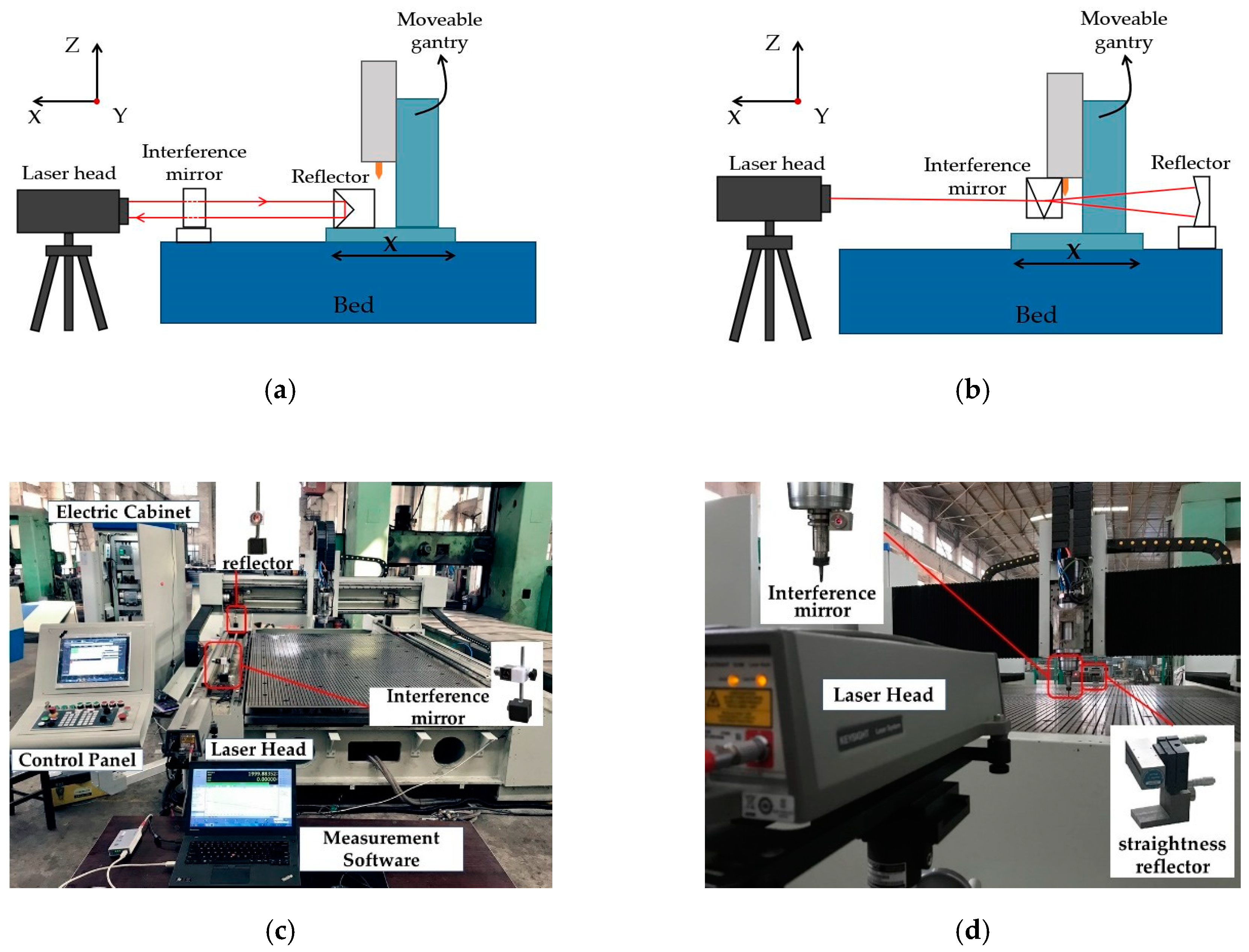
The sample points of the global sensitivity analysis distribute in the unit hypercube space. However, error items are different in scale and the usual sample method may cause inaccuracy in estimating the actual impact of each error item. Thus, a value-leaded factor based on error measurement is proposed to modify the geometric error model, which normalizes errors’ effects to the same level. The Keysight 5530 dual-frequency laser interferometer measurement system is used in the measurement, cooperating with several kinds of mirror groups, 21 geometric errors of the engraving and milling machine can be detected. Measurements are done with the standard of ISO230-1 and the processes are shown in Figure 3. This work includes many time-consuming steps. For each error component, measurement is done in different feed speeds, with the range from 500 mm/min to 6000 mm/min and the interval of 500 mm/min. The measurement stroke is x = 2000 mm, y = 1000 mm, z = 200 mm, which covers the main processing area. The start points are set in x = 200 mm, y = 100 mm and z = 20 mm in machine coordinate system to leave enough space for installing measurement instruments. All the measurements are done for three times. The scale of each error and their ratios are obtained from the measurements. They are used for the normalization of the sample of the global sensitivity analysis. The measured errors are shown in

Table 5. Max error value in the whole stroke.

No.	Item	Max Value	No.	Item	Max Value
1	$\Delta {\mathrm{x}}_{\mathrm{x}}$	0.1212 mm	12	$\Delta {\mathsf{\gamma }}_{\mathrm{y}}$	0.0034 mm/1000 mm
2	$\Delta {\mathrm{y}}_{\mathrm{x}}$	0.0456 mm	13	$\Delta {\mathrm{z}}_{\mathrm{z}}$	0.0218 mm
3	$\Delta {\mathrm{z}}_{\mathrm{x}}$	0.0805 mm	14	$\Delta {\mathrm{x}}_{\mathrm{z}}$	0.0213 mm
4	$\Delta {\mathsf{\alpha }}_{\mathrm{x}}$	0.0037 mm/1000 mm	15	$\Delta {\mathrm{y}}_{\mathrm{z}}$	0.0337 mm
5	$\Delta {\mathsf{\beta }}_{\mathrm{x}}$	0.0032 mm/1000 mm	16	$\Delta {\mathsf{\gamma }}_{\mathrm{z}}$	0.0033 mm/1000 mm
6	$\Delta {\mathsf{\gamma }}_{\mathrm{x}}$	0.0034 mm/1000 mm	17	$\Delta {\mathsf{\beta }}_{\mathrm{z}}$	0.0035 mm/1000 mm
7	$\Delta {\mathrm{y}}_{\mathrm{y}}$	0.0728 mm	18	$\Delta {\mathsf{\alpha }}_{\mathrm{z}}$	0.0036 mm/1000 mm
8	$\Delta {\mathrm{x}}_{\mathrm{y}}$	0.1068 mm	19	$\Delta {\mathsf{\gamma }}_{\mathrm{x}\mathrm{y}}$	0.0125 mm/1000 mm
9	$\Delta {\mathrm{z}}_{\mathrm{y}}$	0.1538 mm	20	$\Delta {\mathsf{\beta }}_{\mathrm{x}\mathrm{z}}$	0.0082 mm/1000 mm
10	$\Delta {\mathsf{\beta }}_{\mathrm{y}}$	0.0036 mm/1000 mm	21	$\Delta {\mathsf{\alpha }}_{\mathrm{y}\mathrm{z}}$	0.0063 mm/1000 mm
11	$\Delta {\mathsf{\alpha }}_{\mathrm{y}}$	0.0037 mm/1000 mm

0.0037 mm/1000 mm means the deviation caused by $\Delta {\mathsf{\alpha }}_{\mathrm{x}}$ in the stroke of 1000 mm is 0.0037 mm. Other angle errors are described in the same way.

.

3.3. Indices Calculation and Global Sensitivity Analysis

The analysis program is made in Matlab according to the steps of the proposed VLGAS method. The geometric error model of the engraving and milling machine built with multi-body system theory is adjusted for normalization based on the error measurement. Putting the model into the analysis program and setting the analysis parameters, the first-order sensitivity indices in three directions are calculated and listed in

Table 6. First-order sensitivity index of each error item.

Number	Item	First-Order Sensitivity
		X-Direction	Y-Direction	Z-Direction
1	$\Delta {\mathrm{x}}_{\mathrm{x}}$	0.333	0.002	0.010
2	$\Delta {\mathrm{y}}_{\mathrm{x}}$	0.004	0.277	0.011
3	$\Delta {\mathrm{z}}_{\mathrm{x}}$	0.006	0.003	0.092
4	$\Delta {\mathsf{\alpha }}_{\mathrm{x}}$	0.000	0.018	0.014
5	$\Delta {\mathsf{\beta }}_{\mathrm{x}}$	0.029	0.003	0.007
6	$\Delta {\mathsf{\gamma }}_{\mathrm{x}}$	0.039	0.007	0.000
7	$\Delta {\mathrm{y}}_{\mathrm{y}}$	0.003	0.424	0.007
8	$\Delta {\mathrm{x}}_{\mathrm{y}}$	0.306	0.027	0.008
9	$\Delta {\mathrm{z}}_{\mathrm{y}}$	0.010	0.000	0.460
10	$\Delta {\mathsf{\beta }}_{\mathrm{y}}$	0.028	0.000	0.007
11	$\Delta {\mathsf{\alpha }}_{\mathrm{y}}$	0.000	0.018	0.008
12	$\Delta {\mathsf{\gamma }}_{\mathrm{y}}$	0.005	0.005	0.000
13	$\Delta {\mathrm{z}}_{\mathrm{z}}$	0.004	0.004	0.297
14	$\Delta {\mathrm{x}}_{\mathrm{z}}$	0.160	0.001	0.003
15	$\Delta {\mathrm{y}}_{\mathrm{z}}$	0.006	0.160	0.007
16	$\Delta {\mathsf{\gamma }}_{\mathrm{z}}$	0.000	0.000	0.000
17	$\Delta {\mathsf{\beta }}_{\mathrm{z}}$	0.000	0.000	0.000
18	$\Delta {\mathsf{\alpha }}_{\mathrm{z}}$	0.000	0.000	0.000
19	$\Delta {\mathsf{\gamma }}_{\mathrm{x}\mathrm{y}}$	0.002	0.058	0.000
20	$\Delta {\mathsf{\beta }}_{\mathrm{x}\mathrm{z}}$	0.027	0.000	0.058
21	$\Delta {\mathsf{\alpha }}_{\mathrm{y}\mathrm{z}}$	0.000	0.018	0.014

The data is drawn and shown in Figure 4 to demonstrate clearly.

.

The angle errors are at a very low level, high-order elements linking to angle errors can be eliminated from the MBS model. Thus, some elements’ sensitivity indices are zero in a particular direction.

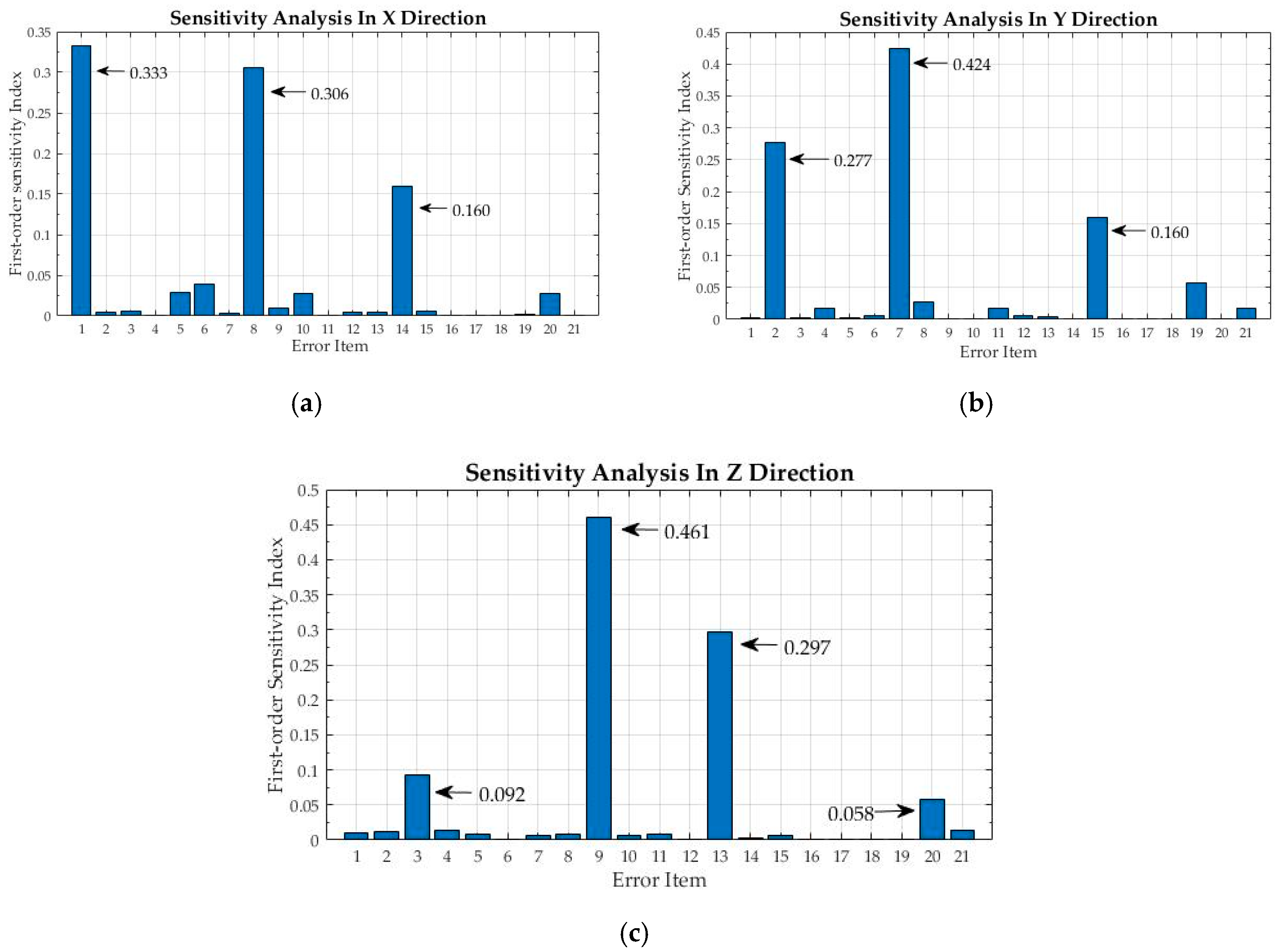
For the X-direction movement, as shown in Figure 4, with the geometric errors changing in a certain range, the sensitivity indices of $\Delta {\mathrm{x}}_{\mathrm{x}}$, $\Delta {\mathrm{x}}_{\mathrm{y}}$ and $\Delta {\mathrm{x}}_{\mathrm{z}}$ are largest and contribute 80% of total value together. For Y direction, the most dominant error element is $\Delta {\mathrm{y}}_{\mathrm{y}}$, which has the highest sensitivity index value of 0.424, the other two dominant error elements are $\Delta {\mathrm{y}}_{\mathrm{x}}$ and $\Delta {\mathrm{y}}_{\mathrm{z}}$, these three elements contribute about 86% of the total value. Similarly, the three linear errors $\Delta {\mathrm{z}}_{\mathrm{x}}$, $\Delta {\mathrm{z}}_{\mathrm{y}}$ and $\Delta {\mathrm{z}}_{\mathrm{z}}$ have the largest impact on the Z direction, with the proportion of around 85%.

In conclusion, for the chosen engraving and milling machine, the dominant errors are mainly linear items, specifically speaking the position error and two straightness errors from the other two feed directions. In other words, compensation aiming at these three errors can provide remarkable improvement to the chosen machine with the minimum cost.

4. Error Compensation

In this section, error data in the whole stroke are listed and modeled based on their character. Different models are applied to a novel real-time compensation system and compared. The linear error in the X direction is chosen as an example. Errors in other directions can be dealt the same way. As shown in the last section, the main error components, which have the largest impact on X-direction linear error, are “X-direction position error,” “X-direction straightness error along with the Y-direction movement” and “X-direction straightness error along with the Z-direction movement.” They all have a close relation to the feed movement, which means they can be compensated by adjusting feed trajectory.

4.1. Position Error Model Based on the Least-Square Method

Position errors are measured three times on each point and the average values are calculated to reduce the measurement error. The error values are listed in

Table 7. Position error in the X direction.

Position (mm)	Error (μm)
	First	Second	Third	Average
0	0	0.012	0.030	0.014
200	−4.797	−6.652	−6.051	−5.833
400	−21.881	−19.252	−18.362	−19.831
600	−32.453	−31.848	−29.204	−31.168
800	−45.158	−40.832	−41.461	−42.483
1000	−59.489	−59.900	−59.560	−59.649
1200	−77.401	−68.519	−63.663	−69.861
1400	−85.961	−80.098	−78.703	−81.587
1600	−95.536	−90.457	−87.197	−91.063
1800	−111.129	−106.270	−98.881	−105.427
2000	−126.542	−118.889	−118.035	−121.155

Origin of the position located on x = 200 mm in machine coordinate system.

,

Table 8. Position error in the Y direction.

Position (mm)	Error (μm)
	First	Second	Third	Average
0	−0.015	−0.035	−0.017	−0.022
100	14.051	14.713	17.019	15.261
200	12.107	11.935	15.522	13.188
300	17.304	17.404	22.221	18.976
400	25.420	25.753	30.710	27.294
500	21.872	22.118	27.867	23.952
600	37.037	37.911	43.779	39.575
700	43.048	43.633	49.924	45.535
800	52.870	54.024	61.151	56.015
900	66.971	68.642	72.338	69.317
1000	71.151	72.285	74.859	72.765

Origin of the position located on y = 100 mm in machine coordinate system.

and

Table 9. Position error in the Z direction.

Position (mm)	Error (μm)
	First	Second	Third	Average
0	0.001	0.053	0.026	0.0267
20	−2.384	−2.422	−2.032	−2.279
40	−4.349	−4.725	−4.561	−4.545
60	−6.437	−6.542	−6.443	−6.474
80	−8.771	−8.713	−8.739	−8.741
100	−10.944	−11.021	−10.867	−10.944
120	−13.196	−13.022	−12.879	−13.032
140	−15.562	−15.469	−15.264	−15.432
160	−17.372	−17.551	−17.411	−17.445
180	−19.198	−19.131	−19.316	−19.215
200	−21.542	−22.037	−21.693	−21.757

Origin of the position located on z = 20 mm in machine coordinate system.

.

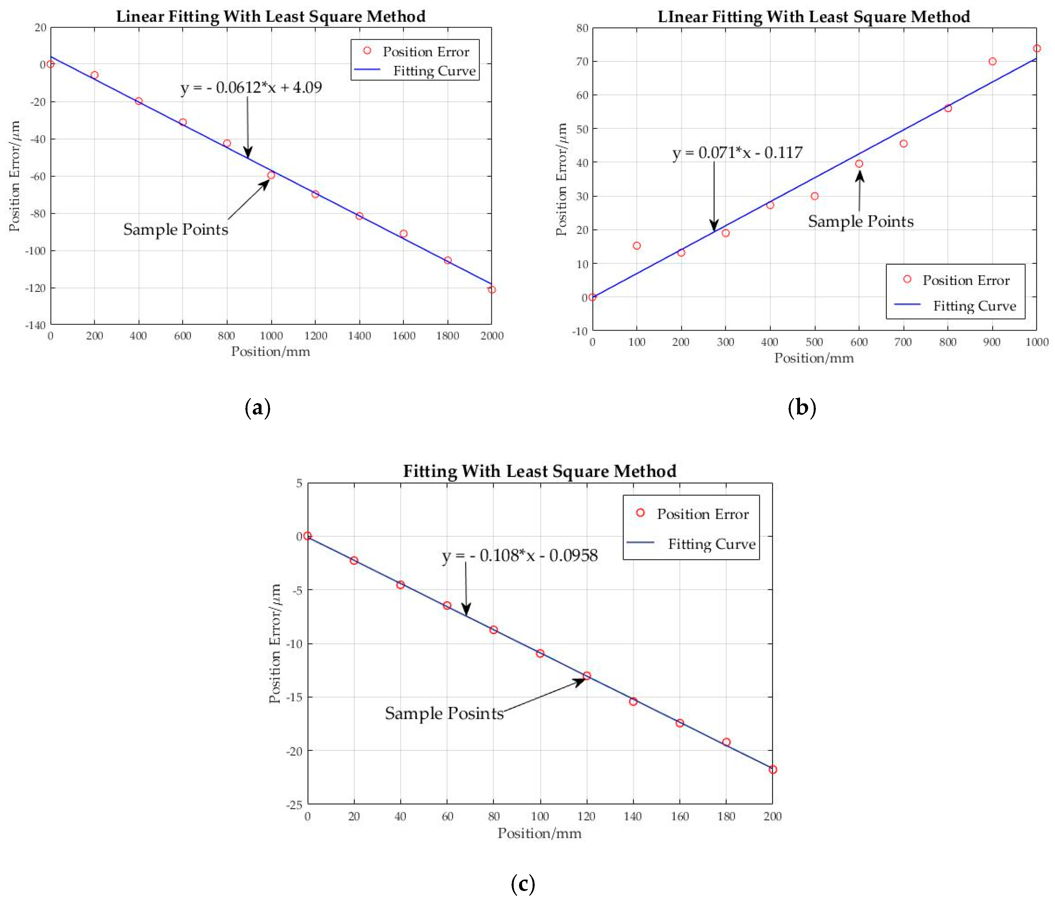
According to the tables, position errors show an obverse trend of linear distribution in the whole stroke. The error value accumulates through the feed movement and the maximum value appears at the end of the stroke. The maximum values in the three directions are −121.155, 72.765 and −19.215, respectively. Thus, the least square method is chosen to establish the mathematical model of the position errors to describe the linear trend.

The least-square method is a commonly used fitting method, in which the fitting curve not necessarily cross the sample points but makes these points as close as possible to the curve. For the sample points (${\mathrm{x}}_{\mathrm{i}}$, ${\mathrm{y}}_{\mathrm{i}}$), a series of equations can be built and used to create the function of the points, the residual sum of squares ${\displaystyle \sum _{\mathrm{i}=1}^{\mathrm{n}}{\mathsf{\delta }}_{\mathrm{i}}^2}$ is chosen to decide the best coefficients of the unknown function. The fitting functions are shown as Equations (28)–(30). The fitting curves of the position errors are shown in Figure 5.

$$\mathrm{y}=-0.0612\mathrm{x}+4.09$$

(28)

$$\mathrm{y}=0.071\mathrm{x}-0.117$$

(29)

$$\mathrm{y}=-0.108\mathrm{x}-0.0958$$

(30)

4.2. Straightness Error Model Based on B-Spline Interpolation.

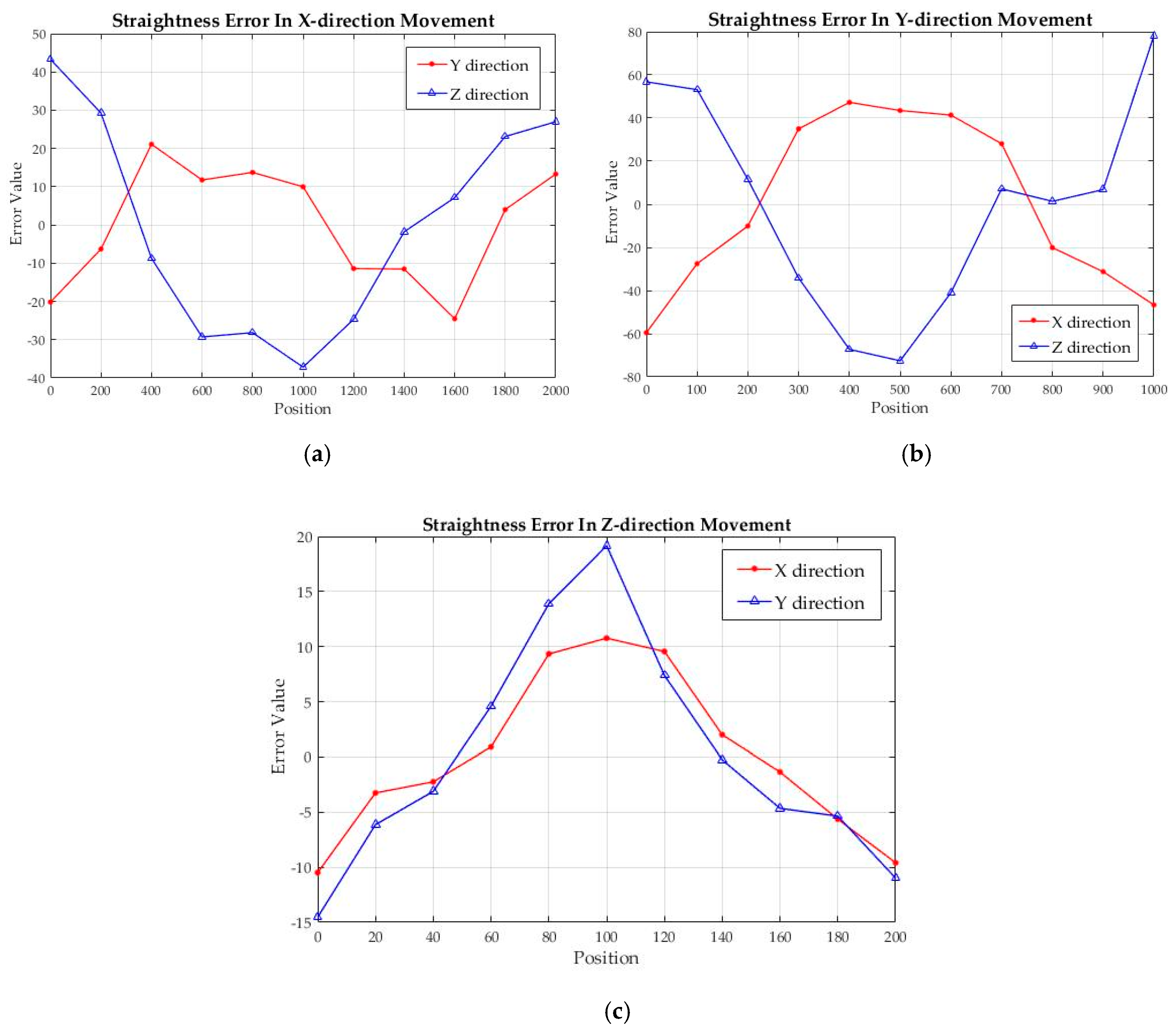
The straightness errors are also measured three times to calculate the average value. The curve of errors is drawn in Figure 6 to show the error intuitively.

According to Figure 6, the max value of the straightness errors is lower than the position errors. The curves fluctuate with the total trend of increasing first and then decreasing, except Y-direction error along with the X-direction movement. The maximum values respectively appear in the point of x₁ = 1600 mm, x₂ = 1000 mm, y₁ = 400 mm, y₂ = 500 mm, z₁ = 100 mm and z₂ = 100 mm for the six straightness errors. The distortion of the guides during manufacturing is the leading cause of straightness errors.

The B-spline curve is a kind of unique curve, which is developed from the Bezier curve and is constructed by the linear combination of B-spline base curves. B-spline curves have many excellent properties, such as geometric invariance, convex hull, convexity retention, variation reduction and local support and so forth. B-spline surface reconstruction is one of the research hotspots and critical technologies of reverse engineering. Therefore, in this paper, the B-spline interpolation is used to establish the mathematical error model of the straightness error, which can describe the continual material property of the guide. The B-spline base function and curve construction function are listed in Appendix A.

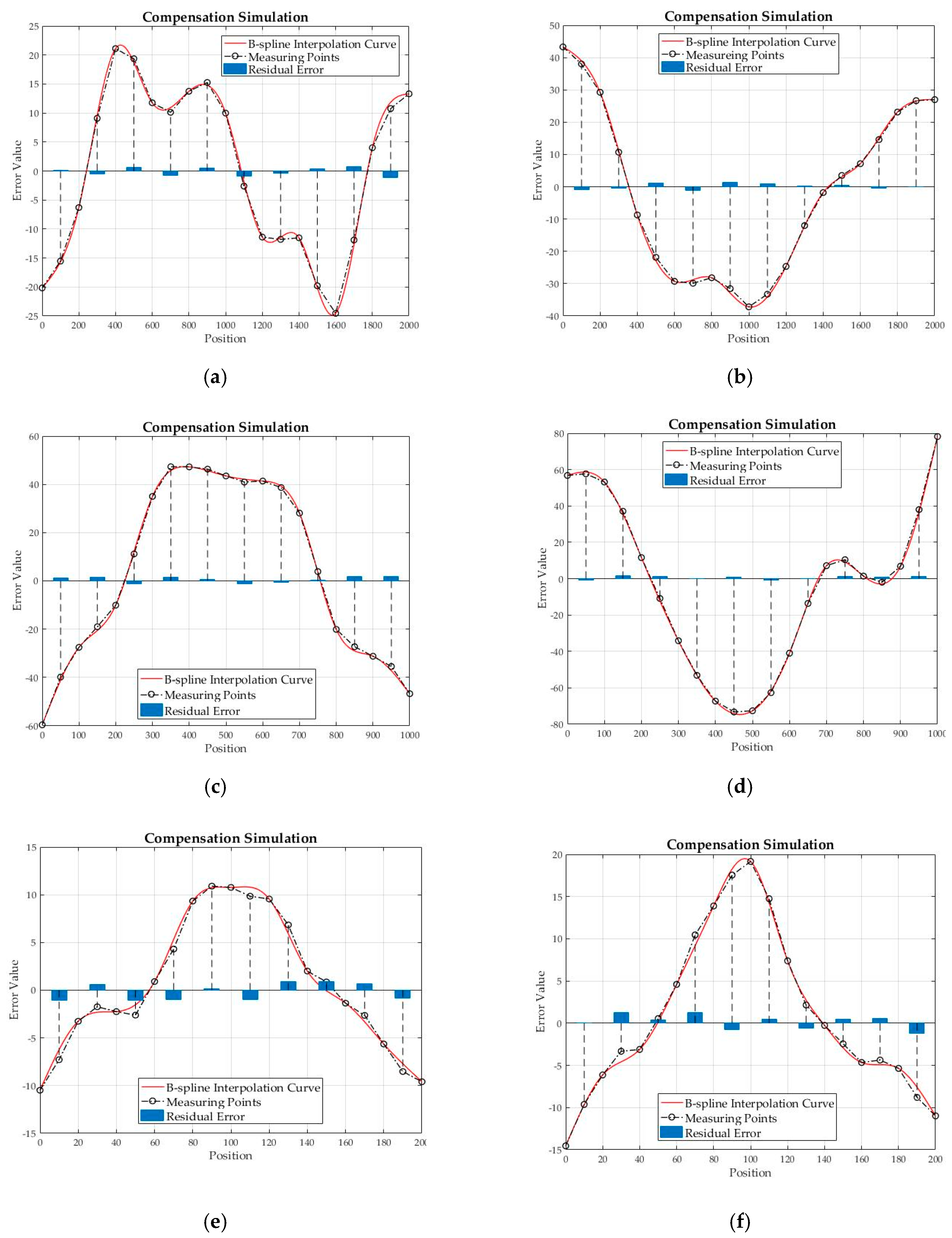
Expanding the measurement point number and doing compensation simulation with the interpolation result, it is shown that the values of residual error keep at a low level after the interpolation and compensation. Interpolation results are shown in Figure 7.

4.3. Compensation System and Experiment

Aiming to error compensation, many researchers in previous works try to change the G code according to the error modeling result, which performs well in reducing the error value [24]. However, this kind of method need pre-work for each program and cannot be real-time. With the advantages of Beckhoff’s open CNC system, the error model can help to improve machine accuracy in a more effective and real-time way.

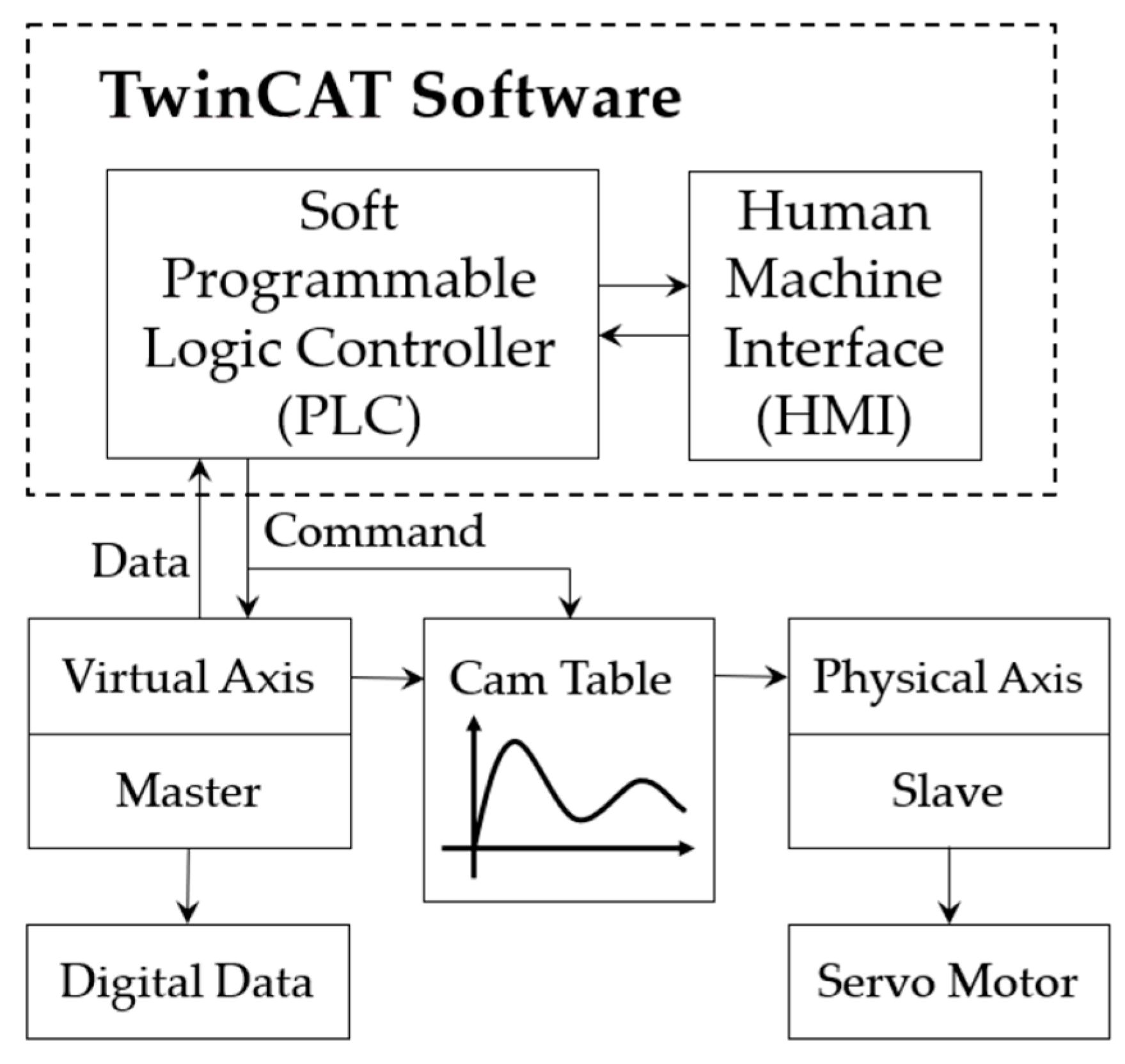
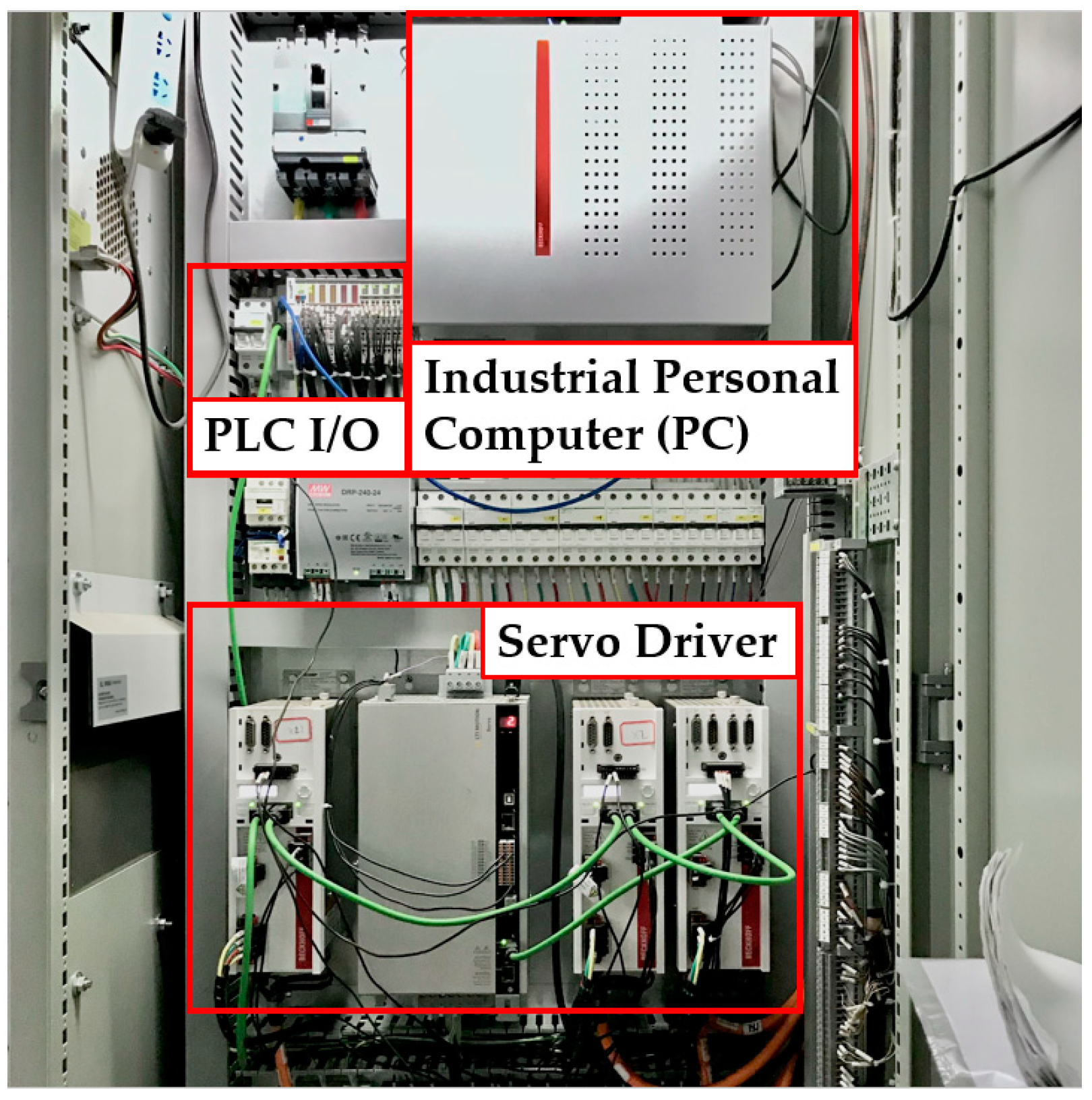
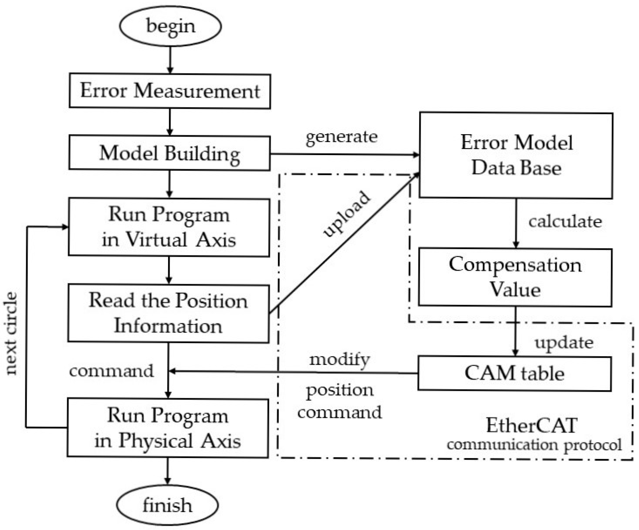
The compensation strategy combines the virtual axis and electronic cam technology based on the TwinCAT control system of Beckhoff. The core of the strategy is uploading error model points into the cam table to help change the actual tool path and offsetting the trajectory deviation. Firstly, a virtual axis is established to accept the motion command. The virtual axis is a kind of electronic symbol in control software. It does not connect to any physical component and only has digital motion simulation. Therefore, it represents the ideal motion state. Secondly, set the virtual axis as the master and create another axis symbol connecting to the physical axis motor as the slave. Thus, the slave axis can move with the master axis, which is the virtual axis and has no physical output, according to specific rules. Thirdly, set the rule between two axes as “electronic cam,” then the physical axis can do superimposed movements of both ideal movements and cam-curve movements based on compensation models. The cam table can be created in two ways: cam design tool assembled in TwinCAT software and user interface linking to soft programmable logic controller (PLC) program. Soft PLC method has better real-time property and the table value can be changed in the feed process. The compensation system can be described in Figure 8. The hardware of the compensation system is shown in Figure 9.

Suppose that x is the ideal position when the feed system moves along the X direction and $\Delta \mathrm{x}$ is the position error generated in the feed stroke, then the cam table value in this position should be set as $-\Delta \mathrm{x}$. Give the motion command to the virtual axis, the electronic cam offset will compensate the error in position x. With the help of the Beckhoff EtherCAT communication system, massive data can be transmitted in real-time. Therefore, coordinate information in all directions can be read and the cam table can be modified with the calculated compensation value based on error models, without delay. The compensation process is expressed in Figure 10.

The compensation system is composed of both hardware and software. The hardware platform of the compensation system is provided by Beckhoff industrial personal computer (PC) and the compensation software is written in C# language. With the Beckhoff ADS communication protocol, data in PLC and Servo controller are easy to be dealt with the algorithm in compensation software and then transmitted back.

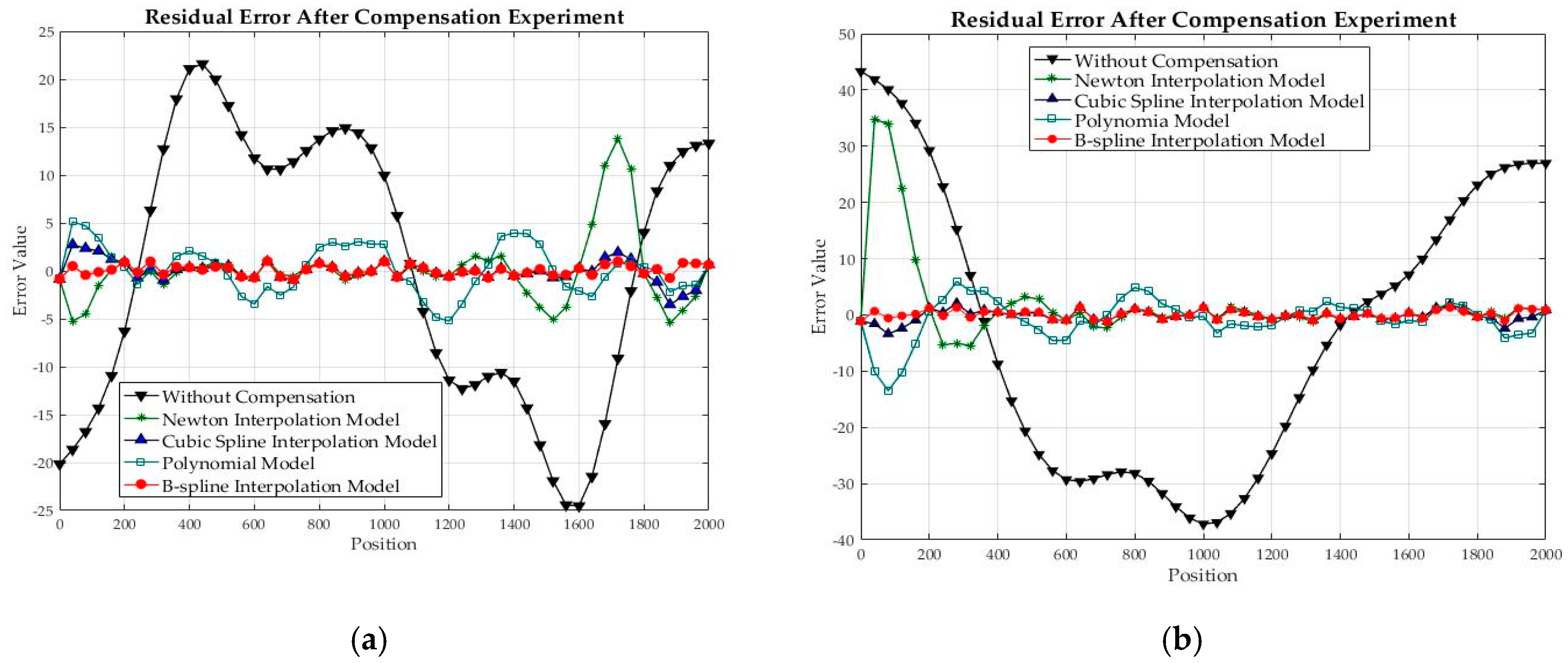
Straightness error after compensation is measured to verify the compensation effect. The error models built by three other usual fitting methods (Polynomial Fitting, Newton Interpolation and Cubic Spline Interpolation) are used to compare with the chosen method of B-spline interpolation. As for the total compensation effect, a space movement of x = 2000 mm, y = 1000 mm and z = 200 mm is carried out and the X-direction total error is measured. The error values are measured by absolute grating rulers. If the total error is curbed at a low level, both the error modeling method and the sensitivity analysis method can be verified to be effective, for only the dominant error components analyzed by the method are compensated. Compensation results are shown in Figure 11.

In Figure 11a,b, the straightness errors along the X-direction movement are shown. The five data curves are respectively the residual error of four chosen compensation models, including the proposed B-spline model and three commonly used fitting models and the error without any compensation. Three comparison models are the Newton interpolation model, the cubic spline interpolation and the polynomial model. From the image, it is obvious that the compensation ability of the B-spline interpolation model is most significant. Newton interpolation model has good performance in the middle part of the stroke but it also shows the Runge’s phenomenon, which leads to huge residual error in the beginning and the end of the movement. The polynomial model has a good ability to follow the trend of the error curve had has a smooth residual error curve. With the polynomial model, the compensation process avoids steep fluctuation of velocity and acceleration. The cubic spline interpolation model has the same capability of eliminating error with the B-spline interpolation model in most positions but still has defects in the beginning and the end of the prediction. The B-spline interpolation method is a kind of sectional interpolation, which means the shape of the interpolation curve only depends on nearby points. Thus, the curve will not be influenced by Runge’s phenomenon. The massive jump of both velocity and acceleration does not exist in the interpolation curve and because of the local adjustable property, the B-spline interpolation can fit irregular error data without influence the fitting of other flat areas. In conclusion, the compensation based on the B-spline interpolation model improves the machine’s straightness accuracy to a remarkable level. The Y-direction and Z-direction straightness errors in the X-direction movement reduce to 2.92 μm and 5.27 μm from 46.55 μm and 80.62 μm. The total straightness accuracy has been improved by around 95%.

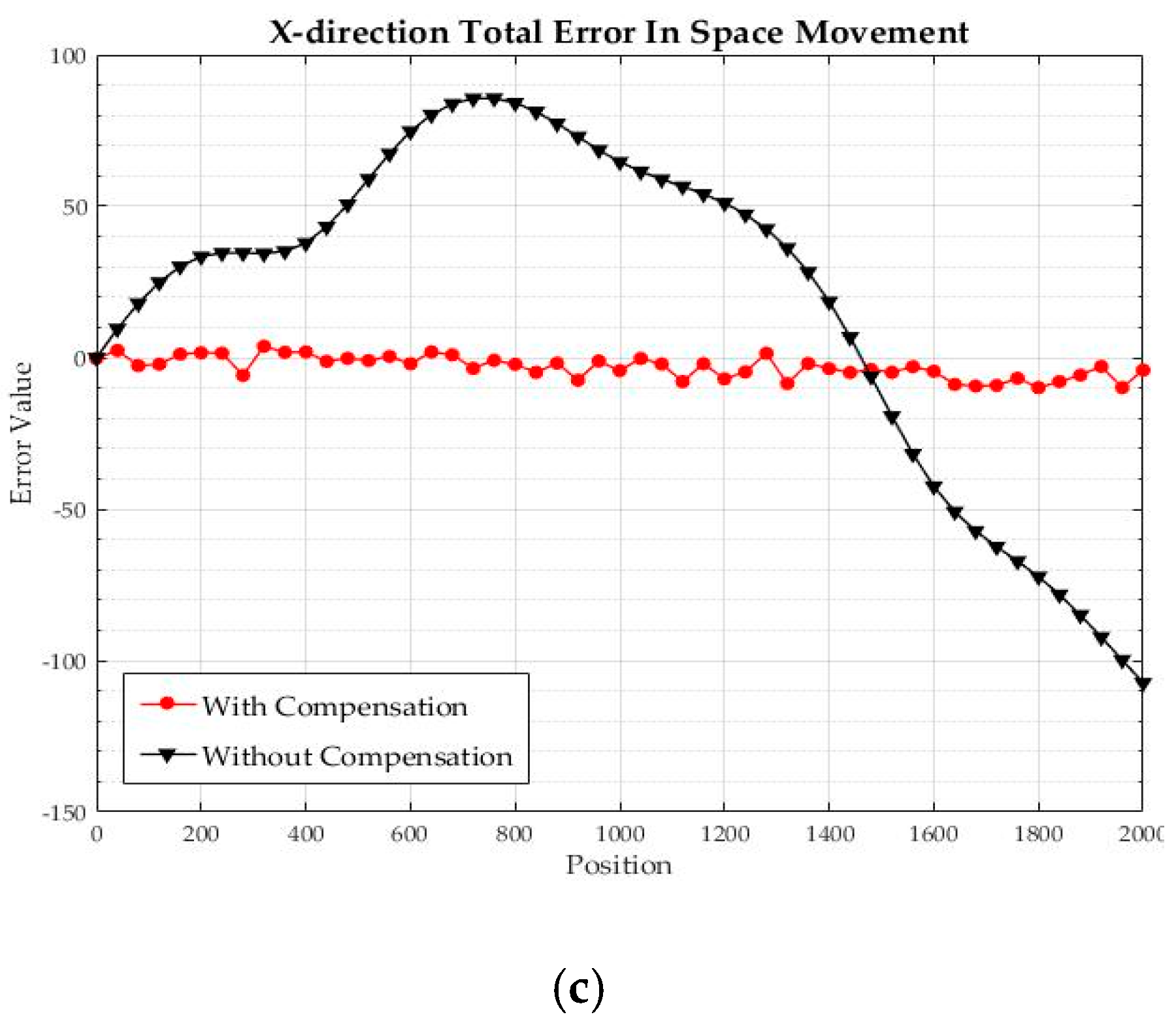
Figure 11c shows the total error of the X-direction position in the space movement with a stroke of x = 2000 mm, y = 1000 mm and z = 200 mm. Two curves respectively show the error before and after compensation. The max value before compensation appears at the end of the stroke, with the error around 110 μm. After compensation, the total error shows a trend of fluctuating enlargement, with the max error of −9.88 μm. In conclusion, after compensation aiming at dominant error components calculated by the VLGSA method, the total error of the X direction in space movement reduces around 90%. The remarkable accuracy improvement of the machine shows the validity of using VLGSA in finding the key errors. Meanwhile, considering the VLGSA method is applied to the MBS model, the model accuracy is also verified.

5. Conclusions

Structural and motional geometric errors widely exist in CNC machines. They are the most common factors reducing the precision machine accuracy, affecting the quality of products. Therefore, characterizing error trends, finding the most dominant error items and finally decreasing total geometric error play an essential role in the development of the modern industry. However, considering the complexity of precision CNC machine tools, the process of targeted compensation can be sophisticated. The following works have been done in this paper to achieve the goal of improving machine accuracy.

• A geometric error model was established with the MBS method. By building the topological structure relationship, the sophisticated error transmitting was decoupled into the calculation of several error matrices, which can be measured separately.
• Based on the MBS error model, error items dominant most to total geometric error were identified by value leaded global sensitivity analysis (VLGSA), in which the actual range of errors was considered in the process of sensitivity analysis. The interaction of different parameters was analyzed in the proposed analysis method.
• Appropriate error fitting methods were applied to measured data. The error data was measured by a high-precision dual-frequency laser interferometer. Considering its excellent ability to describe continual material and significant usage in CAD, the B-spline interpolation method developed on the B-spline curve was used to establish the straightness error model.
• A real-time online compensation system was built based on the Beckhoff TwinCAT servo system. A compensation experiment was carried out using the designed compensation system. The straightness error in the X-direction movement was compensated with four error models to verify the ability of the B-spline interpolation model. The X-direction error in a space movement of x = 2000 mm, y = 1000 mm and z = 200 mm was compensated as a sample. The remarkable reduction of geometric error in X-direction showed the above research was effective.

However, this research is based on the CNC machine operating at a single speed and in cold start temperature. The working condition is more sophisticated in the actual manufacturing process. Thus, further works need to concentrate more on the relationship of geometric errors and the working condition, such as acceleration and changing workforce.

References

- Sarafraz, M.M.; Peyghambarzadeh, S.M. Experimental study on subcooled flow boiling heat transfer to water–diethylene glycol mixtures as a coolant inside a vertical annulus. Exp. Therm. Fluid Science 2013, 50, 154–162. [Google Scholar] [CrossRef]
- Goodarzi, M.; D’Orazio, A.; Keshavarzi, A. Develop the nano scale method of lattice Boltzmann to predict the fluid flow and heat transfer of air in the inclined lid driven cavity with a large heat source inside, Two case studies: Pure natural convection & mixed convection. Phys. Stat. Mech. Appl. 2018, 509, 210–233. [Google Scholar]
- Sarafraz, M.M. Experimental investigation on pool boiling heat transfer to formic acid, propanol and 2-butanol pure liquids under the atmospheric pressure. J. Appl. Fluid Mech. 2013, 6, 73–79. [Google Scholar]
- Goodarzi, M.; Amiri, A.; Goodarzi, M.S. Investigation of heat transfer and pressure drop of a counter flow corrugated plate heat exchanger using MWCNT based nanofluids. Int. Commun. Heat Mass Transf. 2015, 66, 172–179. [Google Scholar] [CrossRef]
- Chen, J.X.; Lin, S.W.; Zhou, X.L. A comprehensive error analysis method for the geometric error of multi-axis machine tool. Int. J. Mach. Tools Manuf. 2016, 106, 56–66. [Google Scholar] [CrossRef]
- Bai, H.; Shen, J.X. Synthesis error modeling of the CNC machine tool based on multi-body system Theory. Aeronaut. Manuf. Technol. 2017, 1, 117–121. [Google Scholar]
- Paul, R.P.; Zhang, H. Computationally efficient kinematics for manipulators with spherical wrists based on the homogeneous transformation representation. Int. J. Robot. Res. 1986, 5, 32–44. [Google Scholar] [CrossRef]
- Veitschegger, W.K.; Wu, C.H. Robot accuracy analysis based on kinematics. IEEE J. Robot. Autom. 1986, 2, 171–178. [Google Scholar] [CrossRef]
- Zhao, Q.Q.; Jun, H.; Liu, Z.G. Modeling method on motive axes error transfer chain for machine tool of arbitrary topological structure. J. Mech. Eng. 2016, 52, 130–137. [Google Scholar] [CrossRef]
- Zhou, X.T. The Research on Machining Accuracy Prediction Based on Machine Tool Error Modeling. Master’s Thesis, Shandong University, Shandong, China, 20 March 2016. [Google Scholar]
- Chhatre, S.; Francis, R.; Zhou, Y.H.; Titchener, H.N.; King, J.; Keshavarz, M.E. Global sensitivity analysis for the determination of parameter importance in bio-manufacturing processes. Biotechnol. Appl. Biochem. 2008, 51, 79–90. [Google Scholar] [CrossRef]
- Cossarini, G.; Solidoro, C. Global sensitivity analysis of a trophodynamic model of the Gulf of Trieste. Ecol. Model. 2008, 212, 16–27. [Google Scholar] [CrossRef]
- Fan, J.W.; Tao, H.H.; Wu, C.J.; Tang, Y.H. Method of error sensitivity analysis of machine tools. J. Beijing Univ. Technol. 2019, 45, 314–320. [Google Scholar]
- Yan, Y.; Wang, G.; Zhang, F.P. Precision assembly geometric error sensitivity analysis based on the error transformation model for precision assembly. Trans. Beijing Inst. Technol. 2017, 37, 682–686. [Google Scholar]
- Li, J.; Xue, F.G.; Liu, X.J. Geometric error modeling and sensitivity analysis of a five-axis machine tool. Int. J. Adv. Manuf. Technol. 2015, 82, 2037–2051. [Google Scholar] [CrossRef]
- Fan, K.G.; Yang, J.G.; Yang, L.Y. Orthogonal polynomials-based thermally induced spindle and geometric error modeling and compensation. Int. J. Adv. Manuf. Technol. 2013, 65, 1791–1800. [Google Scholar] [CrossRef]
- Wang, W.; Zhang, Y.; Yang, J.G. Geometric and thermal error compensation for CNC milling machines based on Newton interpolation method. Proc. Inst. Mech. Eng. Part C J. Mech. Eng. Sci. 2012, 227, 771–778. [Google Scholar] [CrossRef]
- Tuo, Z.Y.; Huang, Y.Q.; Shen, M.W. Modeling of geometric and thermal complex position error of CNC machine tools based on cubic spline interpolation. J. Shanghai Jiao Tong Univ. 2016, 50, 668–672. [Google Scholar]
- Li, Y.H.; Huang, T.; Derek, G.C. An approach for smooth trajectory planning of high-speed pick-and-place parallel robots using quantic B-splines. Mech. Mach. Theory 2018, 126, 479–490. [Google Scholar] [CrossRef] [Green Version]
- Guo, C.; Yang, L.; Li, Q.Y. Modeling of volumetric errors for NC machine tools on multi-body system theories. Mach. Des. Manuf. 2005, 3, 123–125. [Google Scholar]
- Liu, Z.F.; Li, D.D.; Liu, Z.Z. Gantry machining tool assembly method and predictive optimization based on multi-body system. Comput. Integr. Manuf. Syst. 2014, 20, 394–400. [Google Scholar]
- Fan, J.W.; Tang, Y.H.; Wang, H.L. Error modeling and identification technology for a CNC camshaft grinder. J. Vib. Shock 2017, 36, 257–264. [Google Scholar]
- Yu, D.J.; Li, R. Application of Sobol method to sensitivity analysis of a non-linear passive vibration isolators. J. Vib. Eng. 2004, 17, 210–213. [Google Scholar]
- Gao, X.; Tong, H.; Zhou, L. Geometric error compensation of CNC machine tools based on G-code modification. Manuf. Technol. Mach. Tool 2015, 1, 57–62. [Google Scholar]
Figure 1.
Structure of the gantry-moving engraving and milling machine. B0-bed, B1-moveable gantry, B2-Y direction slide, B3-Z direction slide, B4-spindle with the tool, B5-workbench, B6-workpiece. T01–T56 represent the coordinate transformation between the components.
Figure 2.
The topology structure and coordinate definition of the machine. Orange lines show the coordinate transformation between different bodies, which are marked with T01p, T01pe, etc.
Figure 3.
Error measurement. (a) Principle of the position error measurement; (b) Principle of the straightness error measurement; (c) Position error measurement experiment; (d) Straightness error measurement experiment.
Figure 4.
Image of first-order sensitivity index. (a) First-order sensitivity of X-direction error; (b) First-order sensitivity of Y-direction error; (c) First-order sensitivity of Z-direction error.
Figure 5.
Image of fitting curves. (a) Fitting curve of X-direction position error; (b) Fitting curve of Y-direction position error; (c) Fitting curve of Z-direction position error.
Figure 6.
Image of straightness error. (a) Straightness error in the X-direction movement; (b) Straightness error in the Y-direction movement; (c) Straightness error in the Z-direction movement.
Figure 7.
Compensation simulation with B-spline interpolation model. (a) Y-direction straightness error in X-direction movement; (b) Z-direction straightness error in X-direction movement; (c) X-direction straightness error in Y-direction movement; (d) Z-direction straightness error in Y-direction movement; (e) X-direction straightness error in Z-direction movement; (f) Y-direction straightness error in Z-direction movement.
Figure 8.
The structure of the compensation system.
Figure 9.
The hardware of the compensation system.
Figure 10.
The process of the proposed compensation method.
Figure 11.
Compensation experiment result. (a) Residual Y-direction straightness error in X-direction movement before and after compensation; (b) Residual Z-direction straightness error in X-direction movement before and after compensation; (c) Residual X-direction total error before and after compensation.