Guaranteed Lower Bounds for the Elastic Eigenvalues by Using the Nonconforming Crouzeix–Raviart Finite Element

Abstract

This paper uses a locking-free nonconforming Crouzeix–Raviart finite element to solve the planar linear elastic eigenvalue problem with homogeneous pure displacement boundary condition. Making full use of the Poincaré inequality, we obtain the guaranteed lower bounds for eigenvalues. Besides, we also use the nonconforming Crouzeix–Raviart finite element to the planar linear elastic eigenvalue problem with the pure traction boundary condition, and obtain the guaranteed lower eigenvalue bounds. Finally, numerical experiments with MATLAB program are reported.

1. Introduction

The linear elasticity discusses how solid objects deform and become internally stressed under prescribed loading conditions, and is widely used in structural analysis and engineering design. It has been well-known that using the finite element methods for the elasticity equations/eigenvalue problems, the displacement field can be determined numerically. There have been many studies on the finite element methods for the elastic equations/eigenvalue problems (e.g., see [1,2,3,4,5,6,7,8,9,10,11,12,13,14,15,16,17,18,19,20,21,22,23,24,25]). For the elastic equations/eigenvalue problems with pure displacement boundary condition, [1,2,3] studied the conforming finite element methods. As we all know, when $\lambda \to \infty$ (or Poisson ratio $\nu \to \frac{1}{2}$), i.e., the elastic material is nearly incompressible, the locking phenomenon will occur by using the conforming finite elements to solve the equations/eigenvalue problems. In order to overcome the phenomenon of locking, various numerical methods for the linear elasticity equations have been developed. For instance, Brenner et al. [4,5] applied nonconforming Crouzeix–Raviart finite element (CR element). Based on the nonconforming CR element Hansbo [6] proposed a discontinuous Galerkin method, the discontinuous Galerkin method is closely related to the classical nonconforming CR element, which is obtained when one of the stabilizing parameters tends to infinity. Lee et al. [7] proposed a nonconforming Galerkin method based on triangular and quadrilateral elements. Botti et al. [8] constructed a low-order nonconforming approximation method. Rui [9] constructed a finite difference method on staggered grids. Zhang et al. [10] developed the nonconforming virtual element method. Chen et al. [11] presented a nonconforming triangular element and a nonconforming rectangular element. For the elasticity equations with interfaces, Lee [12] adopted the immersed finite element method based on the nonconforming CR element. Jo [13] introduced a low order finite element method for three dimensional elasticity problems. In recent years, mixed nonconforming finite element methods seem to be much more attractive (see [14,15,16,17]), among them, [14,15] studied the linear elasticity equations, [16,17] discussed the elastic eigenvalue problems. Besides, for the pure traction problem, the classical finite element methods can be found in the literature (e.g., see [15,18,19,20,21,22,23,24,25]). In this paper, we apply the nonconforming CR element to the planar linear elastic eigenvalue problem with the pure displacement and the pure traction boundary conditions, and obtain the guaranteed lower bounds for the eigenvalues.

In 1973, Crouzeix and Raviart in [26] first introduced the triangular CR element to solve the stationary Stokes equations. Armentano and Dur$\acute{a}$n in [27] first used the CR element to get the asymptotic lower bounds for the eigenvalues of the Laplace operator. On the basis of their work, finding the asymptotic lower bounds of eigenvalues was further developed by many researchers (e.g., see [28,29,30,31,32,33,34,35,36,37,38]). In recent years, the guaranteed lower bounds for eigenvalues have attracted academic attention. Carstensen in [39] first used the CR element to get the guaranteed lower bounds for eigenvalues of the Laplacian operator. In [40], Carstensen provided a guaranteed lower bounds for the biharmonic operator by nonconforming elements. Li in [41] discussed the guaranteed lower bounds for eigenvalues of the Stokes operator in any dimension. In [42] Liu further developed the work of [39], and gave a framework that provides guaranteed lower eigenvalue bounds for the self-adjoint eigenvalue problems. Later, in [43] Xie et al. presented an guaranteed lower bounds of Stokes eigenvalues by nonconforming elements. You et al. in [44] studied the guaranteed lower bounds for the Steklov eigenvalue problem. Hu et al. in [45] discussed the guaranteed lower bounds for eigenvalues of elliptic operators.

As far as we all know, there is no report on the lower eigenvalue bounds for the elastic eigenvalue problem. Based on the above work, we verify all conditions of the framework of Liu in [42] and apply the framework to the elastic eigenvalue problem, and obtain lower eigenvalue bounds. For the planar linear elastic eigenvalue problem with the pure displacement boundary, we make full use of the Poincaré inequality with an explicit bound in [42] (see (23)) to prove (22) and (26), which is important to lower eigenvalue bounds. We further develop the work of [44] to obtain the guaranteed lower bounds for eigenvalues by using the nonconforming CR element, and prove that is locking-free (see Theorem 1 for details). Besides, we also apply the work of Carstensen in [40] and Liu in [42] to the planar linear elastic eigenvalue problem with the pure traction boundary. We prove that using the nonconforming CR element also can obtain the guaranteed lower bounds for eigenvalues (see Theorem 2 for details), and it can be seen from the numerical experiments that it is locking-free. Further, numerical experiments show that using the linear conforming finite element to solve the planar linear elastic eigenvalue problem with the pure traction boundary is locking-free, this is an interesting phenomenon.

Throughout the paper, C denotes a positive constant independent of the mesh size h and Lamé parameters u and $\lambda$, which may not be the same in different occurrences. The bold letters represent vector-valued operators, functions and associated spaces.

2. The Pure Displacement Problem

Let $\mathbf{x}={(x,y)}^T\in \Omega$, $\Omega \subset {\mathbb{R}}^2$ be a bounded polygonal domain. The standard notation $L^2(\Omega )$ and $W^{s,p}$ are used to denote Lebesgue function space and Sobolev spaces, respectively. For $p=2$, $H^s(\Omega )$ and their associated norms ${\parallel ·\parallel }_{H^s(\Omega )}$ and seminorms ${|·|}_{H^s(\Omega )}$ are used. We denote $H_0^1(\Omega )=\{v\in H^1(\Omega ):v{|}_{\partial \Omega }=0\}$, the space ${\mathbf{L}}^2(\Omega ):=L^2(\Omega )\times L^2(\Omega )$ and Hilbert space ${\mathbf{H}}_0^1(\Omega ):=H_0^1(\Omega )\times H_0^1(\Omega )$. We also define the norms and seminorms on the space ${\mathbf{H}}^s(\Omega )$, for any $\mathbf{v}\left(\mathbf{x}\right)={(v_1\left(\mathbf{x}\right),v_2\left(\mathbf{x}\right))}^T$,

$${\parallel \mathbf{v}\parallel }_{{\mathbf{H}}^s(\Omega )}:={\left({\int }_{\Omega }{\displaystyle \sum _{\alpha \le s}}{\left|{\partial }^{\alpha }\mathbf{v}\right|}^{2}d\mathbf{x}\right)}^{\frac{1}{2}}=\sqrt{\parallel v_1{\parallel }_{H^s(\Omega )}^2+{\parallel v_2\parallel }_{H^s(\Omega )}^2},$$

$${\left|\mathbf{v}\right|}_{{\mathbf{H}}^s(\Omega )}:={\left({\int }_{\Omega }{\displaystyle \sum _{\alpha =s}}{\left|{\partial }^{\alpha }\mathbf{v}\right|}^{2}d\mathbf{x}\right)}^{\frac{1}{2}}=\sqrt{|v_1{|}_{H^s(\Omega )}^2+{\left|v_2\right|}_{H^s(\Omega )}^2}.$$

Let the displacement vector $\mathbf{u}\left(\mathbf{x}\right)={(u_1\left(\mathbf{x}\right),u_2\left(\mathbf{x}\right))}^T$, and the displacement gradient tensor $\nabla \mathbf{u}$ be defined by

$$\nabla \mathbf{u}=\left[\begin{array}{cc}{\partial }_x{u}_1& {\partial }_y{u}_1\\ {\partial }_x{u}_2& {\partial }_y{u}_2\end{array}\right].$$

The strain tensor $ϵ\left(\mathbf{u}\right)$ is defined by

$$ϵ\left(\mathbf{u}\right)=\frac{1}{2}(\nabla \mathbf{u}+{\left(\nabla \mathbf{u}\right)}^T),$$

and the stress tensor $\sigma \left(\mathbf{u}\right)$ is defined by

$$\begin{array}{cc}\hfill \sigma \left(\mathbf{u}\right)& =2\mu ϵ\left(\mathbf{u}\right)+\lambda \mathrm{tr}\left(ϵ\right(\mathbf{u}\left)\right)\mathbf{I},\hfill \\ \hfill & =\left[\begin{array}{c}(2\mu +\lambda ){\partial }_x{u}_1+\lambda {\partial }_y{u}_2\mu ({\partial }_y{u}_1+{\partial }_x{u}_2)\\ \mu ({\partial }_y{u}_1+{\partial }_x{u}_2)(2\mu +\lambda ){\partial }_y{u}_2+\lambda {\partial }_x{u}_1\end{array}\right],\hfill \end{array}$$

where $\mathbf{I}\in {\mathbb{R}}^{2\times 2}$ is the identity matrix, and the positive constants u, $\lambda$ are Lamé parameters given by

$$\mu =\frac{E}{2(1+\nu )},\lambda =\frac{E\nu }{(1+\nu )(1-2\nu )},$$

here the parameter $\nu \in (0,\frac{1}{2})$ is the Poisson ratio and E denotes Young${}^{’}$s modulus. We note that the coefficients $\mu$ and $\lambda$ are $0<{\mu }_1<\mu <{\mu }_2<\infty$ and $0<\lambda <\infty$.

Consider the elastic eigenvalue problem with homogeneous pure displacement boundary condition:

$$\{\begin{array}{c}-\nabla ·\sigma \left(\mathbf{u}\right)=\gamma \rho \mathbf{u},in\Omega ,\\ \mathbf{u}=\mathbf{0},on\partial \Omega ,\end{array}$$

(1)

where $\rho \left(\mathbf{x}\right)$ is the mass density. Without loss of generality, we assume that $\rho \equiv 1$ throughout this paper.

The weak formulation of (1) is: Find $(\gamma ,\mathbf{u})\in \mathbb{R}\times {\mathbf{H}}_0^1(\Omega ),\mathbf{u}\ne \mathbf{0}$, such that

$$a(\mathbf{u},\mathbf{v})=\gamma b(\mathbf{u},\mathbf{v}),\forall \mathbf{v}\in {\mathbf{H}}_0^1(\Omega ),$$

(2)

where

$$\begin{array}{cc}\hfill a(\mathbf{u},\mathbf{v})& ={\int }_{\Omega }\sigma \left(\mathbf{u}\right):\nabla \mathbf{v}d\mathbf{x}\hfill \\ \hfill & =2\mu {\int }_{\Omega }ϵ\left(\mathbf{u}\right):ϵ\left(\mathbf{v}\right)d\mathbf{x}+\lambda {\int }_{\Omega }\left(\mathrm{div}\mathbf{u}\right)\left(\mathrm{div}\mathbf{v}\right)d\mathbf{x}\hfill \\ \hfill & =\mu {\int }_{\Omega }\nabla \mathbf{u}:\nabla \mathbf{v}d\mathbf{x}+(\mu +\lambda ){\int }_{\Omega }\left(\mathrm{div}\mathbf{u}\right)\left(\mathrm{div}\mathbf{v}\right)d\mathbf{x},\hfill \\ \hfill b(\mathbf{u},\mathbf{v})& ={\int }_{\Omega }\rho \mathbf{u}·\mathbf{v}d\mathbf{x},\hfill \end{array}$$

(3)

and $A:B=\mathrm{tr}\left(A{B}^T\right)$ is the Frobenius inner product of matrices A and B, and we use ${\parallel A\parallel }_{{\underset{\sim }{\mathbf{L}}}^2(\Omega )}^2={\int }_{\Omega }A:Ad\mathbf{x}$ to denote the ${\mathbf{L}}^2$-norm of matrix A. From the following Korn${}^{’}$s inequality (see [4], Corollary 11.2.25)

$${\parallel ϵ\left(\mathbf{v}\right)\parallel }_{{\underset{\sim }{\mathbf{L}}}^2(\Omega )}\ge C{\parallel \mathbf{v}\parallel }_{{\mathbf{H}}^1(\Omega )},\forall \mathbf{v}\in {\mathbf{H}}_0^1(\Omega ),$$

(4)

we know that the bilinear form $a(·,·)$ is ${\mathbf{H}}_0^1(\Omega )$-coercive. We use $a(·,·)$ and ${\parallel ·\parallel }_a=\sqrt{a(·,·)}$ as an inner product and norm on ${\mathbf{H}}_0^1(\Omega )$, respectively, use $b(·,·)$ and ${\parallel ·\parallel }_{{\mathbf{L}}^2(\Omega )}=\sqrt{b(·,·)}$ as an inner product and norm on ${\mathbf{L}}^2(\Omega )$, respectively.

Let ${\pi }_h:=\left\{\kappa \right\}$ be a regular triangular mesh of $\Omega$, and the mesh diameter $h=\underset{\kappa \in {\pi }_h}{\max }{h}_{\kappa }$ where $h_{\kappa }$ is the diameter of element $\kappa$. Let the set of all interior edges of ${\pi }_h$ as ${\epsilon }_h^i$, the set of the edges on the boundary as ${\epsilon }_h^b$ and ${\epsilon }_h={\epsilon }_h^i\cup {\epsilon }_h^b$.

The the nonconforming CR element ${\mathbf{V}}_h(\Omega )$ is defined by

$${\mathbf{V}}_h(\Omega ):=V_h(\Omega )\times V_h(\Omega ),$$

where

$$\begin{array}{cc}\hfill V_h(\Omega )& =\{v\in L^2(\Omega ):v{|}_{\kappa }\in \mathrm{span}\{1,x,y\},\kappa \in {\pi }_h;{\int }_{e}v{|}_{{\kappa }_1}ds={\int }_{e}v{|}_{{\kappa }_2}ds,\hfill \\ \hfill & \forall e\in {\epsilon }_h^i,\partial {\kappa }_1\cap \partial {\kappa }_2=e;{\int }_{e}vds=0,\forall e\in {\epsilon }_h^b\}.\hfill \end{array}$$

For any $\mathbf{v}\in {\mathbf{V}}_h(\Omega )$ we define $\left({\nabla }_h\mathbf{v}\right){|}_{\kappa }=\nabla \left(\mathbf{v}{|}_{\kappa }\right)$, $\left({\mathrm{div}}_h\mathbf{v}\right){|}_{\kappa }=\mathrm{div}\left(\mathbf{v}{|}_{\kappa }\right)$ and $\left({\Delta }_h\mathbf{v}\right){|}_{\kappa }=\Delta \left(\mathbf{v}{|}_{\kappa }\right)$.

For the nonconforming CR element, the interpolation operator $I_h:H_0^1(\Omega )\to V_h(\Omega )$ is defined by

$${\int }_e(v-I_{h}v)ds=0,\forall e\in {\epsilon }_h,v\in H_0^1(\Omega ).$$

(5)

Define

$${\mathbf{I}}_h\mathbf{v}:=(I_h{v}_1,I_h{v}_2)\in {\mathbf{V}}_h(\Omega ),\forall \mathbf{v}=(v_1,v_2).$$

Then operator ${\mathbf{I}}_h:{\mathbf{H}}_0^1(\Omega )\to {\mathbf{V}}_h(\Omega )$, and

$${\int }_e(\mathbf{v}-{\mathbf{I}}_h\mathbf{v})ds=0,\forall e\in {\epsilon }_h,\mathbf{v}\in {\mathbf{H}}_0^1(\Omega ).$$

(6)

Denote

$$\mathbf{H}\left(h\right)={\mathbf{V}}_h(\Omega )+{\mathbf{H}}_0^1(\Omega )=\{{\mathbf{v}}_h+\mathbf{v}:{\mathbf{v}}_h\in {\mathbf{V}}_h(\Omega ),\mathbf{v}\in {\mathbf{H}}_0^1(\Omega )\}.$$

The nonconforming CR element approximation of (2) is: Find $({\gamma }_h,{\mathbf{u}}_h)\in \mathbb{R}\times {\mathbf{V}}_h(\Omega )$, $\parallel {\mathbf{u}}_h{\parallel }_{{\mathbf{L}}^2(\Omega )}=1$, satisfying

$$a_h({\mathbf{u}}_h,{\mathbf{v}}_h)={\gamma }_{h}b({\mathbf{u}}_h,{\mathbf{v}}_h),\forall {\mathbf{v}}_h\in {\mathbf{V}}_h(\Omega ),$$

(7)

where

$$a_h({\mathbf{u}}_h,{\mathbf{v}}_h)=\mu {\int }_{\Omega }{\nabla }_h{\mathbf{u}}_h:{\nabla }_h{\mathbf{v}}_{h}d\mathbf{x}+(\mu +\lambda ){\int }_{\Omega }\left({\mathrm{div}}_h{\mathbf{u}}_h\right)\left({\mathrm{div}}_h{\mathbf{v}}_h\right)d\mathbf{x}.$$

Korn’s inequality for piecewise $H^1$-vector fields (see [20]) plays an important role in the existence and uniqueness of the solution for the linear elasticity problem discreted by the discontinuous Galerkin method. For the nonconforming CR element, discrete Equation (7) has a unique solution because $a_h(·,·)$ is positive definite (see page 325 in [4]). In fact, the nonconforming bilinear form $a_h(·,·)$ is symmetric and positive definite on $\mathbf{H}\left(h\right)$. Because $a_h({\mathbf{v}}_h,{\mathbf{v}}_h)=0$ implies that ${\mathbf{v}}_h$ is piecewise constant, and the zero boundary condition together with continuity at the midpoints imply ${\mathbf{v}}_h\equiv \mathbf{0}$.

Define the nonconforming energy norm ${\parallel ·\parallel }_h$ and the norm ${|·|}_{1,h}$ on $\mathbf{H}\left(h\right)$, respectively:

$${\parallel \mathbf{v}\parallel }_h=\sqrt{a_h(\mathbf{v},\mathbf{v})},$$

$${\left|\mathbf{v}\right|}_{1,h}=\sqrt{{\displaystyle \sum _{\kappa \in {\pi }_h}}{\left|\mathbf{v}\right|}_{{\mathbf{H}}^1\left(\kappa \right)}^2},$$

and

$${\left|\mathbf{v}\right|}_{1,h}=\sqrt{{\displaystyle \sum _{\kappa \in {\pi }_h}}{\left|\mathbf{v}\right|}_{{\mathbf{H}}^1\left(\kappa \right)}^2}=\sqrt{{\sum }_{\kappa \in {\pi }_h}{\int }_{\kappa }\nabla \mathbf{v}:\nabla \mathbf{v}d\mathbf{x}}\le C{\parallel \mathbf{v}\parallel }_h.$$

(8)

Consider the associated boundary value problem of (2) and discrete form:

$$\mathbf{w}\in {\mathbf{H}}_0^1(\Omega ),a(\mathbf{w},\mathbf{v})=b(\mathbf{f},\mathbf{v}),\forall \mathbf{v}\in {\mathbf{H}}_0^1(\Omega ).$$

(9)

$${\mathbf{w}}_h\in {\mathbf{V}}_h(\Omega ),a_h({\mathbf{w}}_h,\mathbf{v})=b(\mathbf{f},\mathbf{v}),\forall \mathbf{v}\in {\mathbf{V}}_h(\Omega ).$$

(10)

where $\mathbf{f}={(f_1\left(\mathbf{x}\right),f_2\left(\mathbf{x}\right))}^T\in {\mathbf{L}}^2(\Omega )$ is the body force.

Let $\Omega \subset {\mathbb{R}}^2$ be a bounded convex polygonal domain, from (11.4.4) in [4] (or Lemma 2.2 in [5]) we have the elliptic regularity estimate:

For any $\mathbf{f}\in {\mathbf{L}}^2(\Omega )$, (9) exists a unique solution $\mathbf{w}\in {\mathbf{H}}^2(\Omega )\cap {\mathbf{H}}_0^1(\Omega )$ satisfying

$${\parallel \mathbf{w}\parallel }_{{\mathbf{H}}^2(\Omega )}+{\lambda \parallel \mathrm{div}\mathbf{w}\parallel }_{{\mathbf{H}}^1(\Omega )}\le C_{\Omega }{\parallel \mathbf{f}\parallel }_{{\mathbf{L}}^2(\Omega )},$$

(11)

where the positive constant $C_{\Omega }$ is independent of Lamé parameters $\mu$ and $\lambda$.

The above inequality (11) plays an essential role in showing the robustness of our numerical approximation to (9).

Brenner et al. in [4,5] studied and proved the following estimates:

Proposition 1.

Let $\Omega \subset {\mathbb{R}}^2$ be a bounded convex polygonal domain, $\mathbf{w}$ and ${\mathbf{w}}_h$ be the kth eigenvalues of (9) and (10), respectively. There exists a positive constant C such that

$$\parallel {\mathbf{w}}_h{-\mathbf{w}\parallel }_h\le Ch{\parallel \mathbf{f}\parallel }_{{\mathbf{L}}^2(\Omega )},$$

(12)

$$\parallel {\mathbf{w}}_h{-\mathbf{w}\parallel }_{{\mathbf{L}}^2(\Omega )}\le C{h}^2{\parallel \mathbf{f}\parallel }_{{\mathbf{L}}^2(\Omega )},$$

(13)

where C is independent of h and $(\mu ,\lambda )$, which indicates that the nonconforming CR element method is locking-free.

Proof of Proposition 1.

See the proof method of Theorem 3.1 on page 331 and Theorem 3.2 on page 332 in [5] or the proof method of Theorem 11.4.15 on page 325 in [4] to prove (12) and (13). □

Define the operator $\mathbf{T}:{\mathbf{L}}^2(\Omega )\to {\mathbf{H}}_0^1(\Omega )\hookrightarrow {\mathbf{L}}^2(\Omega )$ such that

$$a(\mathbf{T}\mathbf{f},\mathbf{v})=b(\mathbf{f},\mathbf{v}),\forall \mathbf{v}\in {\mathbf{H}}_0^1(\Omega ),$$

(14)

and ${\mathbf{T}}_h:{\mathbf{L}}^2(\Omega )\to {\mathbf{V}}_h(\Omega )\neg \subseteq {\mathbf{H}}_0^1(\Omega )$ such that

$$a_h({\mathbf{T}}_h\mathbf{f},\mathbf{v})=b(\mathbf{f},\mathbf{v}),\forall \mathbf{v}\in {\mathbf{V}}_h(\Omega ).$$

(15)

Then both $\mathbf{T}$ and ${\mathbf{T}}_h$ are self-adjoint and completely continuous operators. (2) and (7) have the following equivalent operator forms, respectively:

$$\begin{array}{c}\mathbf{T}\mathbf{u}={\gamma }^{-1}\mathbf{u},\\ {\mathbf{T}}_h{\mathbf{u}}_h={\gamma }_h^{-1}{\mathbf{u}}_h.\end{array}$$

Proposition 2.

Let $\Omega \subset {\mathbb{R}}^2$ be a bounded convex polygonal domain, $({\gamma }_h,{\mathbf{u}}_h)$ be the kth eigenpair of (7), and $\parallel {\mathbf{u}}_h{\parallel }_{{\mathbf{L}}^2(\Omega )}=1$, γ be the kth eigenvalue of (2). Then ${\gamma }_h\to \gamma (h\to 0)$, and there exists an eigenfunction $\mathbf{u}$ corresponding to γ, ${\parallel \mathbf{u}\parallel }_{{\mathbf{L}}^2(\Omega )}=1$, such that

$$\parallel {\mathbf{u}}_h{-\mathbf{u}\parallel }_h\le Ch,$$

(16)

$$\parallel {\mathbf{u}}_h{-\mathbf{u}\parallel }_{{\mathbf{L}}^2(\Omega )}\le C{h}^2,$$

(17)

where the positive constant C is independent of h and $(\mu ,\lambda )$, i.e., the nonconforming CR element method is locking-free.

Proof of Proposition 2. 

From (13) we know

$$\parallel {\mathbf{T}}_h{-\mathbf{T}\parallel }_{{\mathbf{L}}^2(\Omega )}=\underset{\mathbf{f}\in {\mathbf{L}}^2(\Omega )\setminus \left\{\mathbf{0}\right\}}{\sup }\frac{\parallel {\mathbf{T}}_h{\mathbf{f}-\mathbf{T}\mathbf{f}\parallel }_{{\mathbf{L}}^2(\Omega )}}{{\parallel \mathbf{f}\parallel }_{{\mathbf{L}}^2(\Omega )}}\le C{h}^2\to 0(h\to 0).$$

From the spectral approximation theory, we have ${\gamma }_h\to \gamma (h\to 0)$. According to Lemma 2.3 in [32] we get

$$\parallel {\mathbf{u}}_h{-\mathbf{u}\parallel }_{{\mathbf{L}}^2(\Omega )}\le C{\parallel ({\mathbf{T}}_h-\mathbf{T})\mathbf{u}\parallel }_{{\mathbf{L}}^2(\Omega )},$$

$$\parallel {\mathbf{u}}_h{-\mathbf{u}\parallel }_h=\gamma {\parallel ({\mathbf{T}}_h-\mathbf{T})\mathbf{u}\parallel }_h+R,$$

where $R\le C\parallel ({\mathbf{T}}_h-\mathbf{T}){\mathbf{u}\parallel }_{{\mathbf{L}}^2(\Omega )}$.

Let $\mathbf{f}=\mathbf{u}$ in (9) and (10), then $\mathbf{w}=\mathbf{T}\mathbf{u},{\mathbf{w}}_h={\mathbf{T}}_h\mathbf{u}$. Since

$$\begin{array}{c}\parallel {\mathbf{u}}_h{-\mathbf{u}\parallel }_{{\mathbf{L}}^2(\Omega )}\le C{\parallel {\mathbf{w}}_h-\mathbf{w}\parallel }_{{\mathbf{L}}^2(\Omega )},\hfill \\ \parallel {\mathbf{u}}_h{-\mathbf{u}\parallel }_h\le \gamma \parallel {\mathbf{w}}_h{-\mathbf{w}\parallel }_h+C{\parallel {\mathbf{w}}_h-\mathbf{w}\parallel }_{{\mathbf{L}}^2(\Omega )},\hfill \end{array}$$

which, together with (12) and (13), yields (16) and (17). □

The Lower Bounds for the Eigenvalues of the Pure Displacement Problem

In [42] Liu established a framework that provides guaranteed lower eigenvalue bounds for the self-adjoint eigenvalue problems. We verify all conditions of the framework and apply it to obtain lower bounds for the eigenvalues of the planar linear elastic eigenvalue problem with the pure displacement boundary.

A1 

V is a Hilbert space of real function on $\Omega$ with the inner product $M(·,·)$ and the corresponding norm ${\parallel ·\parallel }_M:=\sqrt{M(·,·)}$.

A2 

$N(·,·)$ is another inner product of V. The corresponding norm ${\parallel ·\parallel }_N:=\sqrt{N(·,·)}$ is compact for V with respect to ${\parallel ·\parallel }_M$, i.e., every sequence in V which is bounded in ${\parallel ·\parallel }_M$ has a subsequence, which is Cauchy in ${\parallel ·\parallel }_N$.

A3 

$V^h$ is a finite dimensional space of real function over $\Omega$, Dim($V^h$) = n. Define $V\left(h\right):=V+V^h=\{v+v_h|v\in V,v_h\in V^h\}$.

A4 

Bilinear forms $M_h(·,·)$ and $N_h(·,·)$ on $V\left(h\right)$ are extension of $M(·,·)$ and $N(·,·)$ to $V\left(h\right)$, such that

(1)

$M_h(u,v)=M(u,v),N_h(u,v)=N(u,v)$, $\forall u,v\in V$.

(2)

$M_h(·,·)$ and $N_h(·,·)$ are symmetric and positive definite on $V\left(h\right)$.

The assumption A4 means that $M_h(·,·)$ and $N_h(·,·)$ are inner products of $V\left(h\right)$. In order to simplicity, the extended bilinear forms $M_h(·,·)$ and $N_h(·,·)$ are still denoted by $M(·,·)$ and $N(·,·)$, and the corresponding norms are denoted by ${\parallel ·\parallel }_M$ and ${\parallel ·\parallel }_N$, respectively.

Under the above assumptions, in [42] Liu gave the following Lemma.

Lemma 1

(the Theorem 2.1 in [42]). Suppose that γ and ${\gamma }_h$ are the kth eigenvalues of (2) and (7), respectively, $P_h:V\left(h\right)\to V^h$ is the projection, $\forall u\in V\left(h\right)$

$$M(u-P_{h}u,v_h)=0,\forall v_h\in V^h.$$

(18)

Suppose the following error estimation holds, $\forall u\in V$

$$\parallel u-P_h{u\parallel }_N\le C_h{\parallel u-P_{h}u\parallel }_M.$$

(19)

Then, there holds

$$\frac{{\gamma }_{h,i}}{1+{\gamma }_{h,i}{C}_h^2}\le {\gamma }_i(i=1,2,\cdots ,n).$$

(20)

For the pure displacement problem, we take the following settings:

$$\begin{array}{c}\mathbf{V}:={\mathbf{H}}_0^1(\Omega ),{\mathbf{V}}^h:={\mathbf{V}}_h(\Omega ),\\ M(·,·):=a_h(·,·),N(·,·):={b(·,·),\parallel ·\parallel }_M:={\parallel ·\parallel }_h{,\parallel ·\parallel }_N:={\parallel ·\parallel }_{{\mathbf{L}}^2(\Omega )}.\end{array}$$

It is easy to verify that the above settings satisfy the assumption $\mathbf{A}\mathbf{1}-\mathbf{A}\mathbf{4}$. In the following discussion, for consistency of notations, we use ${\mathbf{H}}_0^1(\Omega )$, ${\mathbf{V}}_h(\Omega )$, $\mathbf{H}\left(h\right)$, $a_h(·,·)$, $b(·,·)$, ${\parallel ·\parallel }_h$, ${\parallel ·\parallel }_{{\mathbf{L}}^2(\Omega )}$ to denote $\mathbf{V}$, ${\mathbf{V}}^h$, $V\left(h\right)$, $M(·,·)$, $N(·,·)$, ${\parallel ·\parallel }_M,{\parallel ·\parallel }_N$, respectively.

Theorem 1

(guaranteed lower bounds for eigenvalues). Let ${\gamma }_k$ and ${\gamma }_{h,k}$ be the kth eigenvalue of (2) and (7), respectively, then the following guaranteed lower bounds holds

$${\underline{\gamma }}_{h,k}\le {\gamma }_k(k=1,2,\cdots ,n),$$

(21)

where ${\underline{\gamma }}_{h,k}=\frac{{\gamma }_{h,k}}{1+{\gamma }_{h,k}{C}_h^2}$, $C_h=0.346h\frac{1}{\sqrt{\mu }}$.

Proof of Theorem 1.

For any $\mathbf{u}\in \mathbf{H}\left(h\right)$, ${\mathbf{v}}_h\in {\mathbf{V}}_h(\Omega )$, using integration by parts and noticing that $\frac{\partial {\mathbf{v}}_h}{\partial \mathbf{n}}$ is a constant function on edges ($\mathbf{n}$ is the unit outward normal vector), ${\mathbf{v}}_h$ is a linear function on element $\kappa$ and ${\Delta }_h{\mathbf{v}}_h=0$, which together with (6) we have

$$\begin{array}{cc}\hfill & a_h(\mathbf{u}-{\mathbf{I}}_h\mathbf{u},{\mathbf{v}}_h)\hfill \\ \hfill & =\mu {\int }_{\Omega }{\nabla }_h(\mathbf{u}-{\mathbf{I}}_h\mathbf{u}):{\nabla }_h{\mathbf{v}}_{h}d\mathbf{x}+(\mu +\lambda ){\int }_{\Omega }{\mathrm{div}}_h(\mathbf{u}-{\mathbf{I}}_h\mathbf{u})\left({\mathrm{div}}_h{\mathbf{v}}_h\right)d\mathbf{x}\hfill \\ \hfill & =\mu ({\int }_{\Omega }-{\Delta }_h{\mathbf{v}}_h(\mathbf{u}-{\mathbf{I}}_h\mathbf{u})d\mathbf{x}+{\displaystyle \sum _{e\in {\epsilon }_h}}{\int }_e(\mathbf{u}-{\mathbf{I}}_h\mathbf{u})\frac{\partial {\mathbf{v}}_h}{\partial \mathbf{n}}ds)\hfill \\ \hfill & +(\mu +\lambda )({\int }_{\Omega }-{\nabla }_h\left({\mathrm{div}}_h{\mathbf{v}}_h\right)(\mathbf{u}-{\mathbf{I}}_h\mathbf{u})d\mathbf{x}+{\displaystyle \sum _{e\in {\epsilon }_h}}{\int }_e(\mathbf{u}-{\mathbf{I}}_h\mathbf{u})\frac{\partial {\mathbf{v}}_h}{\partial \mathbf{n}}ds)\hfill \\ \hfill & =0,\hfill \end{array}$$

(22)

thus the interpolation operator ${\mathbf{I}}_h$ is the orthogonal projection.

For $\kappa \in {\pi }_h$, the edges of which are denoted by $e_1,e_2,e_3$, let

$${\mathbf{V}}_e\left(\kappa \right)=\{\mathbf{v}\in {\mathbf{H}}^1\left(\kappa \right):{\int }_{e_i}\mathbf{v}ds=0,i=1,2,3\}.$$

The following the Poincaré inequality with an explicit bound (see Theorem 3.2 in [42]) plays an crucial role in studying guaranteed lower eigenvalue bounds.

$${\parallel \mathbf{v}\parallel }_{{\mathbf{L}}^2\left(\kappa \right)}\le 0.346h_{\kappa }{\left|\mathbf{v}\right|}_{{\mathbf{H}}^1\left(\kappa \right)},\forall \mathbf{v}\in {\mathbf{V}}_e\left(\kappa \right).$$

(23)

Since $\mathbf{u}-{\mathbf{I}}_h\mathbf{u}\in {\mathbf{V}}_e\left(\kappa \right)$, by (23) we get

$$\parallel \mathbf{u}-{\mathbf{I}}_h{\mathbf{u}\parallel }_{{\mathbf{L}}^2\left(\kappa \right)}\le 0.346h_{\kappa }{|\mathbf{u}-{\mathbf{I}}_h\mathbf{u}|}_{{\mathbf{H}}^1\left(\kappa \right)},$$

(24)

then

$$\begin{array}{c}\parallel \mathbf{u}-{\mathbf{I}}_h{\mathbf{u}\parallel }_{{\mathbf{L}}^2(\Omega )}^2\le \frac{1}{\mu }{\displaystyle \sum _{\kappa \in {\pi }_h}}{\left(0.346h_{\kappa }\right)}^2\mu {|\mathbf{u}-{\mathbf{I}}_h\mathbf{u}|}_{{\mathbf{H}}^1\left(\kappa \right)}^2\hfill \\ \le \frac{1}{\mu }{\left(0.346h\right)}^2\{{\displaystyle \sum _{\kappa \in {\pi }_h}}\mu |\mathbf{u}-{\mathbf{I}}_h{\mathbf{u}|}_{{\mathbf{H}}^1\left(\kappa \right)}^2+(\mu +\lambda ){\parallel \mathrm{div}(\mathbf{u}-{\mathbf{I}}_h\mathbf{u})\parallel }_{{\mathbf{L}}^2(\Omega )}^2\},\hfill \end{array}$$

(25)

thus we have

$$\parallel \mathbf{u}-{\mathbf{I}}_h{\mathbf{u}\parallel }_{{\mathbf{L}}^2(\Omega )}\le 0.346h\frac{1}{\sqrt{\mu }}{\parallel \mathbf{u}-{\mathbf{I}}_h\mathbf{u}\parallel }_h.$$

(26)

Taking $P_h={\mathbf{I}}_h$, $C_h=0.346h\frac{1}{\sqrt{\mu }}$, and combining (22), (26) and Lemma 1 we deduce (21). □

Remark 1.

Actually, when the angles of meshes meet contain condition (see Theorem 4.2 in [42] for details), such as uniform meshes used in our numerical experiments, the value of $C_h$ can be $0.1893h\frac{1}{\sqrt{\mu }}$.

3. The Pure Traction Problem

In this section, we present the nonconforming CR finite element for the planar linear elastic eigenvalue problem with the pure traction boundary condition. Unless explicitly noted in this section, we use the same notation as in Section 2.

We consider the planar linear elastic eigenvalue problem with the pure traction boundary:

$$\{\begin{array}{c}-\nabla ·\sigma \left(\mathbf{u}\right)=\gamma \rho \mathbf{u},in\Omega ,\\ \sigma \left(\mathbf{u}\right)\mathbf{n}=\mathbf{0},on\partial \Omega ,\end{array}$$

(27)

where $\mathbf{n}$ is the unit outward normal vector with respect to the domain $\Omega$.

The weak formulation of (27) can be described as to find $(\omega ,\mathbf{u})\in \mathbb{R}\times {\mathbf{H}}^1(\Omega )$ such that

$$a(\mathbf{u},\mathbf{v})=\omega b(\mathbf{u},\mathbf{v}),\forall \mathbf{v}\in {\mathbf{H}}^1(\Omega ),$$

(28)

where $\omega =\gamma +1$ and

$$\begin{array}{cc}\hfill a(\mathbf{u},\mathbf{v})& ={\int }_{\Omega }\sigma \left(\mathbf{u}\right):\nabla \mathbf{v}d\mathbf{x}+{\int }_{\Omega }\rho \mathbf{u}·\mathbf{v}d\mathbf{x}\hfill \\ \hfill & =2\mu {\int }_{\Omega }\epsilon \left(\mathbf{u}\right):\epsilon \left(\mathbf{v}\right)d\mathbf{x}+\lambda {\int }_{\Omega }\left(\mathrm{div}\mathbf{u}\right)\left(\mathrm{div}\mathbf{v}\right)d\mathbf{x}+{\int }_{\Omega }\rho \mathbf{u}·\mathbf{v}d\mathbf{x}\hfill \\ \hfill & =\mu {\int }_{\Omega }\nabla \mathbf{u}:\nabla \mathbf{v}d\mathbf{x}+(\mu +\lambda ){\int }_{\Omega }\left(\mathrm{div}\mathbf{u}\right)\left(\mathrm{div}\mathbf{v}\right)d\mathbf{x}+{\int }_{\Omega }\rho \mathbf{u}·\mathbf{v}d\mathbf{x},\hfill \\ \hfill b(\mathbf{u},\mathbf{v})& ={\int }_{\Omega }\rho \mathbf{u}·\mathbf{v}d\mathbf{x}.\hfill \end{array}$$

By the Korn’s inequality (see [4], Theorem 11.2.16)

$${\parallel ϵ\left(\mathbf{v}\right)\parallel }_{{\underset{\sim }{\mathbf{L}}}^2(\Omega )}+{\parallel \mathbf{v}\parallel }_{{\mathbf{L}}^2(\Omega )}\ge C{\parallel \mathbf{v}\parallel }_{{\mathbf{H}}^1(\Omega )},\forall \mathbf{v}\in {\mathbf{H}}^1(\Omega ),$$

(29)

we can know that the bilinear form $a(·,·)$ is ${\mathbf{H}}^1(\Omega )$-coercive. We use $a(·,·)$ and ${\parallel ·\parallel }_a=\sqrt{a(·,·)}$ as an inner product and norm on ${\mathbf{H}}^1(\Omega )$, respectively.

Let $V_h(\Omega )$ be the nonconforming CR element space:

$$\begin{array}{cc}\hfill V_h(\Omega )& =\{v\in L^2(\Omega ):v{|}_{\kappa }\in \mathrm{span}\{1,x,y\},\kappa \in {\pi }_h;{\int }_{e}v{|}_{{\kappa }_1}ds={\int }_{e}v{|}_{{\kappa }_2}ds,\hfill \\ \hfill & \forall e\in {\epsilon }_h^i,\partial {\kappa }_1\cap \partial {\kappa }_2=e\}.\hfill \end{array}$$

Denote ${\mathbf{V}}_h(\Omega )=V_h(\Omega )\times V_h(\Omega )$, and

$$\mathbf{H}\left(h\right)={\mathbf{V}}_h(\Omega )+{\mathbf{H}}^1(\Omega )=\{{\mathbf{v}}_h+\mathbf{v}:{\mathbf{v}}_h\in {\mathbf{V}}_h(\Omega ),\mathbf{v}\in {\mathbf{H}}^1(\Omega )\}.$$

The nonconforming CR element approximation of (28) is: Find $({\omega }_h,{\mathbf{u}}_h)\in \mathbb{R}\times {\mathbf{V}}_h(\Omega )$, satisfying

$$a_h({\mathbf{u}}_h,{\mathbf{v}}_h)={\omega }_{h}b({\mathbf{u}}_h,{\mathbf{v}}_h),\forall {\mathbf{v}}_h\in {\mathbf{V}}_h(\Omega ),$$

(30)

where ${\omega }_k={\gamma }_k+1$ and

$$a_h({\mathbf{u}}_h,{\mathbf{v}}_h)=\mu {\int }_{\Omega }{\nabla }_h{\mathbf{u}}_h:{\nabla }_h{\mathbf{v}}_{h}d\mathbf{x}+(\mu +\lambda ){\int }_{\Omega }\left({\mathrm{div}}_h{\mathbf{u}}_h\right)\left({\mathrm{div}}_h{\mathbf{v}}_h\right)d\mathbf{x}+{\int }_{\Omega }\rho {\mathbf{u}}_h·{\mathbf{v}}_{h}d\mathbf{x}.$$

It is easy to know that the nonconforming bilinear form $a_h(·,·)$ is symmetric and positive definite on $\mathbf{H}\left(h\right)$.

Define the nonconforming energy norm ${\parallel ·\parallel }_h$ and the norm ${|·|}_{1,h}$ on $\mathbf{H}\left(h\right)$, respectively:

$${\parallel \mathbf{v}\parallel }_h=\sqrt{a_h(\mathbf{v},\mathbf{v})},{\left|\mathbf{v}\right|}_{1,h}=\sqrt{{\displaystyle \sum _{\kappa \in {\pi }_h}}{\left|\mathbf{v}\right|}_{{\mathbf{H}}^1\left(\kappa \right)}^2},$$

and

$${\left|\mathbf{v}\right|}_{1,h}=\sqrt{{\displaystyle \sum _{\kappa \in {\pi }_h}}{\int }_{\kappa }\nabla \mathbf{v}:\nabla \mathbf{v}d\mathbf{x}}\le C{\parallel \mathbf{v}\parallel }_h.$$

Consider the associated boundary value problem of (28) and discrete form:

$$\mathbf{w}\in {\mathbf{H}}^1(\Omega ),a(\mathbf{w},\mathbf{v})=b(\mathbf{f},\mathbf{v}),\forall \mathbf{v}\in {\mathbf{H}}^1(\Omega ).$$

(31)

$${\mathbf{w}}_h\in {\mathbf{V}}_h(\Omega ),a_h({\mathbf{w}}_h,\mathbf{v})=b(\mathbf{f},\mathbf{v}),\forall \mathbf{v}\in {\mathbf{V}}_h(\Omega ).$$

(32)

Define the operator $\mathbf{K}:{\mathbf{H}}^1(\Omega )\to {\mathbf{H}}^1(\Omega )\hookrightarrow {\mathbf{L}}^2(\Omega )$ such that

$$a(\mathbf{K}\mathbf{f},\mathbf{v})=b(\mathbf{f},\mathbf{v}),\forall \mathbf{v}\in {\mathbf{H}}^1(\Omega ),$$

(33)

and ${\mathbf{K}}_h:{\mathbf{V}}_h(\Omega )\to {\mathbf{V}}_h(\Omega )\neg \subseteq {\mathbf{H}}^1(\Omega )$ such that

$$a_h({\mathbf{K}}_h\mathbf{f},\mathbf{v})=b(\mathbf{f},\mathbf{v}),\forall \mathbf{v}\in {\mathbf{V}}_h(\Omega ).$$

(34)

Then both $\mathbf{K}$ and ${\mathbf{K}}_h$ are self-adjoint and completely continuous operators.

The Lower Bounds for Eigenvalues of the Pure Traction Problem

For the elastic eigenvalue problem with the pure traction boundary condition, we also use ${\mathbf{H}}^1(\Omega )$, ${\mathbf{V}}_h(\Omega )$, $\mathbf{H}\left(h\right)$ $a_h(·,·)$, $b(·,·)$, ${\parallel ·\parallel }_h$, ${\parallel ·\parallel }_{{\mathbf{L}}^2(\Omega )}$ to denote $\mathbf{V}$, ${\mathbf{V}}^h$, $V\left(h\right)$, $M(·,·)$, $N(·,·)$, ${\parallel ·\parallel }_M,{\parallel ·\parallel }_N$, respectively, which also satisfy the assumption A1–A4.

Let ${\mathbf{P}}_h:\mathbf{H}\left(h\right)\to {\mathbf{V}}_h(\Omega )$ be the projection operator. For $\mathbf{u}\in \mathbf{H}\left(h\right)$, ${\mathbf{P}}_h\mathbf{u}$ satisfies

$$a_h(\mathbf{u}-{\mathbf{P}}_h\mathbf{u},{\mathbf{v}}_h)=0,\forall {\mathbf{v}}_h\in {\mathbf{V}}_h(\Omega ).$$

(35)

Using the argument in [44] we give the estimate between the interpolation and projection operators.

Lemma 2.

Let ${\mathbf{I}}_h:{\mathbf{H}}^1(\Omega )\to {\mathbf{V}}_h(\Omega )$ be the interpolation operator of the nonconforming CR element, for all $\mathbf{u}\in \mathbf{H}\left(h\right)$, we have

$$\parallel {\mathbf{I}}_h\mathbf{u}-{\mathbf{P}}_h{\mathbf{u}\parallel }_{{\mathbf{L}}^2(\Omega )}\le \frac{1}{\sqrt{{\omega }_{h,1}}}{\parallel {\mathbf{I}}_h\mathbf{u}-\mathbf{u}\parallel }_{{\mathbf{L}}^2(\Omega )}.$$

(36)

Proof of Lemma 2.

For the convenience of readers, we refer to the Lemma 3.6 in [44] to give a detailed proof. From (34), for any ${\mathbf{\Phi }}_h\in {\mathbf{V}}_h(\Omega )$, we have ${\mathbf{K}}_h{\mathbf{\Phi }}_h\in {\mathbf{V}}_h(\Omega )$ and

$$a_h({\mathbf{K}}_h{\mathbf{\Phi }}_h,{\mathbf{v}}_h)=b({\mathbf{\Phi }}_h,{\mathbf{v}}_h),\forall {\mathbf{v}}_h\in {\mathbf{V}}_h(\Omega ).$$

(37)

Let ${\mathbf{v}}_h:={\mathbf{K}}_h{\mathbf{\Phi }}_h$ in the above formula, then

$$\parallel {\mathbf{K}}_h{\mathbf{\Phi }}_h{\parallel }_h^2=b({\mathbf{\Phi }}_h,{\mathbf{K}}_h{\mathbf{\Phi }}_h)\le \parallel {\mathbf{\Phi }}_h{\parallel }_{{\mathbf{L}}^2(\Omega )}{\parallel {\mathbf{K}}_h{\mathbf{\Phi }}_h\parallel }_{{\mathbf{L}}^2(\Omega )}.$$

(38)

From the definition of ${\omega }_{h,1}$ in (30) and the min–max principle, we get

$${\omega }_{h,1}\le \frac{\parallel {\mathbf{K}}_h{\mathbf{\Phi }}_h{\parallel }_h^2}{\parallel {\mathbf{K}}_h{\mathbf{\Phi }}_h{\parallel }_{{\mathbf{L}}^2(\Omega )}^2},$$

(39)

which together with (38) yields the estimate

$$\parallel {\mathbf{K}}_h{\mathbf{\Phi }}_h{\parallel }_h\le \frac{1}{\sqrt{{\omega }_{h,1}}}{\parallel {\mathbf{\Phi }}_h\parallel }_{{\mathbf{L}}^2(\Omega )}.$$

(40)

For any $\mathbf{u}\in \mathbf{H}\left(h\right)$, using the same argument as (22) we get

$$\begin{array}{cc}\hfill a_h({\mathbf{I}}_h\mathbf{u}-\mathbf{u},{\mathbf{v}}_h)& =\mu {\int }_{\Omega }{\nabla }_h({\mathbf{I}}_h\mathbf{u}-\mathbf{u}):{\nabla }_h{\mathbf{v}}_{h}d\mathbf{x}\hfill \\ \hfill & +(\mu +\lambda ){\int }_{\Omega }{\mathrm{div}}_h({\mathbf{I}}_h\mathbf{u}-\mathbf{u})\left({\mathrm{div}}_h{\mathbf{v}}_h\right)d\mathbf{x}+{\int }_{\Omega }\rho ({\mathbf{I}}_h\mathbf{u}-\mathbf{u})·{\mathbf{v}}_{h}d\mathbf{x}\hfill \\ \hfill & ={\int }_{\Omega }\rho ({\mathbf{I}}_h\mathbf{u}-\mathbf{u})·{\mathbf{v}}_{h}d\mathbf{x}.\hfill \end{array}$$

(41)

Let ${\mathbf{v}}_h:={\mathbf{I}}_h\mathbf{u}-{\mathbf{P}}_h\mathbf{u}$ and ${\mathbf{\Psi }}_h:={\mathbf{K}}_h{\mathbf{v}}_h\in {\mathbf{V}}_h(\Omega )$. Combining (35), (37) and $\rho \equiv 1$ we have

$$\begin{array}{cc}\hfill \parallel {\mathbf{v}}_h{\parallel }_{{\mathbf{L}}^2(\Omega )}^2& =b({\mathbf{v}}_h,{\mathbf{v}}_h)\hfill \\ \hfill & =a_h({\mathbf{\Psi }}_h,{\mathbf{I}}_h\mathbf{u}-\mathbf{u}+\mathbf{u}-{\mathbf{P}}_h\mathbf{u})=a_h({\mathbf{\Psi }}_h,{\mathbf{I}}_h\mathbf{u}-\mathbf{u}).\hfill \end{array}$$

(42)

Let ${\mathbf{v}}_h={\mathbf{\Psi }}_h$ in (41), together with (40) and (42) we obtain

$$\begin{array}{cc}\hfill \parallel {\mathbf{v}}_h{\parallel }_{{\mathbf{L}}^2(\Omega )}^2=& {\int }_{\Omega }\rho ({\mathbf{I}}_h\mathbf{u}-\mathbf{u})·{\mathbf{\Psi }}_{h}d\mathbf{x}\le \parallel {\mathbf{\Psi }}_h{\parallel }_{{\mathbf{L}}^2(\Omega )}{\parallel {\mathbf{I}}_h\mathbf{u}-\mathbf{u}\parallel }_{{\mathbf{L}}^2(\Omega )}\hfill \\ \hfill & \le \parallel {\mathbf{\Psi }}_h{\parallel }_h{\parallel {\mathbf{I}}_h\mathbf{u}-\mathbf{u}\parallel }_{{\mathbf{L}}^2(\Omega )}\hfill \\ \hfill & \le \frac{1}{\sqrt{{\omega }_{h,1}}}\parallel {\mathbf{v}}_h{\parallel }_{{\mathbf{L}}^2(\Omega )}{\parallel {\mathbf{I}}_h\mathbf{u}-\mathbf{u}\parallel }_{{\mathbf{L}}^2(\Omega )}.\hfill \end{array}$$

(43)

From (43) we can immediately obtain (36). □

Theorem 2

(guaranteed lower bounds for eigenvalues). Let ${\omega }_k$ and ${\omega }_{h,k}$ be as defined in (28) and (30), respectively. Then, there holds

$${\underline{\omega }}_{h,k}\le {\omega }_k(k=1,2,\cdots ,n),$$

(44)

where ${\underline{\omega }}_{h,k}=\frac{{\omega }_{h,k}}{1+{\omega }_{h,k}{C}_h^2},C_h=(\frac{1}{\sqrt{{\omega }_{h,1}}}+1)0.346h\frac{1}{\sqrt{\mu }}$.

Proof of Theorem 2.

For any $\mathbf{u}\in \mathbf{H}\left(h\right)$, from (23) we get the following estimates:

$$\begin{array}{cc}\hfill \parallel \mathbf{u}-{\mathbf{I}}_h{\mathbf{u}\parallel }_{{\mathbf{L}}^2(\Omega )}& \le {\left({\displaystyle \sum _{\kappa \in {\pi }_h}}{\left(0.346h_{\kappa }\right)}^2{|\mathbf{u}-{\mathbf{I}}_h\mathbf{u}|}_{{\mathbf{H}}^1\left(\kappa \right)}^2\right)}^{1/2}\hfill \\ \hfill & \le 0.346\underset{\kappa \in {\pi }_h}{\max }{h}_{\kappa }{|\mathbf{u}-{\mathbf{I}}_h\mathbf{u}|}_{1,h}.\hfill \end{array}$$

(45)

From the triangle inequality, (36) and (45) we obtain

$$\begin{array}{cc}\hfill \parallel \mathbf{u}-{\mathbf{P}}_h{\mathbf{u}\parallel }_{{\mathbf{L}}^2(\Omega )}& \le \parallel \mathbf{u}-{\mathbf{I}}_h{\mathbf{u}\parallel }_{{\mathbf{L}}^2(\Omega )}+{\parallel {\mathbf{I}}_h\mathbf{u}-{\mathbf{P}}_h\mathbf{u}\parallel }_{{\mathbf{L}}^2(\Omega )}\hfill \\ \hfill & \le (1+\frac{1}{\sqrt{{\omega }_{h,1}}}){\parallel \mathbf{u}-{\mathbf{I}}_h\mathbf{u}\parallel }_{{\mathbf{L}}^2(\Omega )}\hfill \\ \hfill & \le (1+\frac{1}{\sqrt{{\omega }_{h,1}}})0.346\underset{\kappa \in {\pi }_h}{\max }{h}_{\kappa }{|\mathbf{u}-{\mathbf{I}}_h\mathbf{u}|}_{1,h}\hfill \\ \hfill & \le C_h{|\mathbf{u}-{\mathbf{P}}_h\mathbf{u}|}_{1,h}\hfill \\ \hfill & \le C_h{\parallel \mathbf{u}-{\mathbf{P}}_h\mathbf{u}\parallel }_h,\forall \mathbf{u}\in {\mathbf{V}}_h(\Omega ),\hfill \end{array}$$

(46)

here $C_h=(\frac{1}{\sqrt{{\omega }_{h,1}}}+1)0.346h\frac{1}{\sqrt{\mu }}$, $h=\underset{\kappa \in {\pi }_h}{\max }{h}_{\kappa }$.

From Lemma 1 we can immediately obtain (44). □

Remark 2.

Same as Remark 1, when the angles of meshes meet contain condition the value of $C_h$ can be $(\frac{1}{\sqrt{{\omega }_{h,1}}}+1)0.1893h\frac{1}{\sqrt{\mu }}$.

4. Numerical Experiments

In this section, we report some numerical experiments. In our computation, our program was completed under the package of iFEM [46], and the discrete eigenvalue problems were solved in MATLAB 2012a on a DELL inspiron 5480 PC with 8G memory, and the MATLAB codes are in Appendix A. The following notations are adopted in tables.

h: the meshes $h=\underset{\kappa \in {\pi }_h}{\max }{h}_{\kappa }$.

${\gamma }_{h,k}$: the kth eigenvalue of (7) obtained by the nonconforming CR element.

${\underline{\gamma }}_{h,k}$: the approximation obtained by correcting ${\gamma }_{h,k}$, i.e., the lower bounds of the kth eigenvalue of (1) or (27).

${\gamma }_{h,k}^c$: the kth eigenvalue obtained by the linear conforming finite element.

${\underline{\gamma }}_{glb}$: guaranteed lower bounds for the elastic eigenvalues.

cond${}_2$(CR): the condition number of the stiffness matrix of (30) obtained by the nonconforming CR element.

cond${}_2$(P1): the condition number of the stiffness matrix obtained by the linear conforming element.

Example 1.

Consider the planar linear elastic eigenvalue problem with the pure displacement boundary condition (1), we take the mass density $\rho =1$, Lamé parameter $\mu =1$ and take $\lambda =1,\lambda =100,\lambda ={10}^4,\lambda ={10}^8$, respectively.

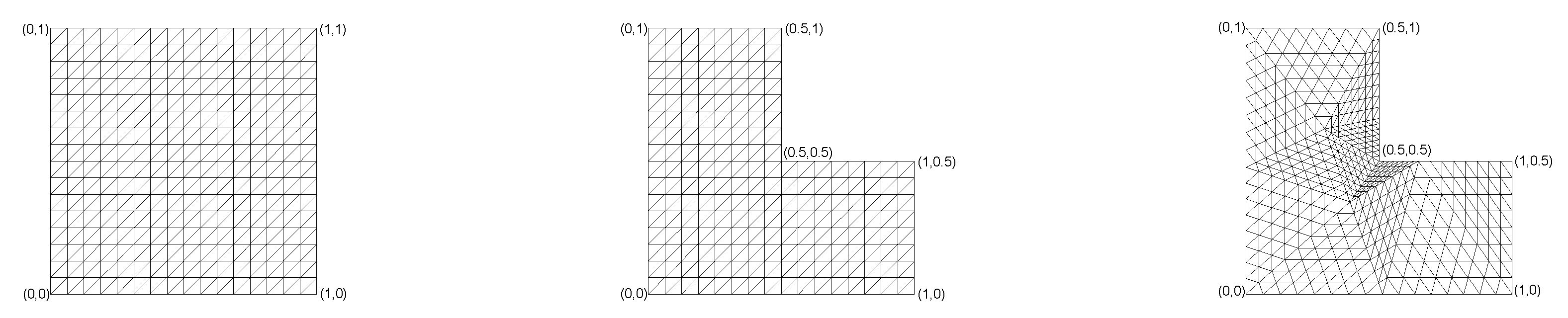
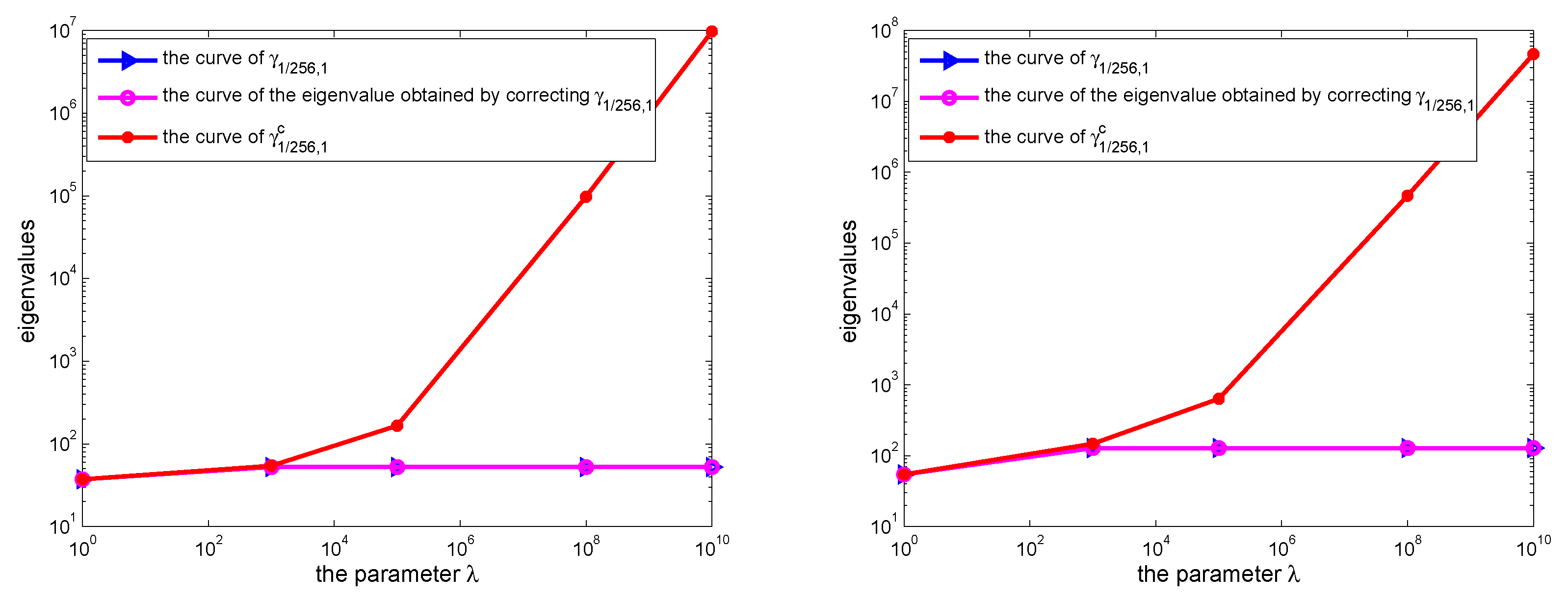
We use the nonconforming CR element to solve (1) on the unit square ${\Omega }_S={[0,1]}^2$ and L-shaped domain ${\Omega }_L={[0,1]}^2\backslash {[\frac{1}{2},1]}^2$, respectively. On each domain, we select two eigenvalues to execute correction. One is the minimum eigenvalue, and the other is selected because it is an upper bound of the exact value on the coarsest mesh. For the uniform meshes, $C_h=0.1893h\frac{1}{\sqrt{\mu }}$ is used for the results in

Table 1. The first selected eigenvalue on the uniform meshes for ${\Omega }_S$.

h	$\mathit{\lambda }=1$		$\mathit{\lambda }=100$		$\mathit{\lambda }={10}^4$		$\mathit{\lambda }={10}^8$
	${\underline{\mathit{\gamma }}}_{\mathit{h},\mathbf{1}}$	${\mathit{\gamma }}_{\mathit{h},\mathbf{1}}$	${\underline{\mathit{\gamma }}}_{\mathit{h},\mathbf{1}}$	${\mathit{\gamma }}_{\mathit{h},\mathbf{1}}$	${\underline{\mathit{\gamma }}}_{\mathit{h},\mathbf{1}}$	${\mathit{\gamma }}_{\mathit{h},\mathbf{1}}$	${\underline{\mathit{\gamma }}}_{\mathit{h},\mathbf{1}}$	${\mathit{\gamma }}_{\mathit{h},\mathbf{1}}$
$\frac{\sqrt{2}}{2}$	17.886861	26.322914	19.651300	30.330628	19.692868	30.429766	19.693293	30.430780
$\frac{\sqrt{2}}{4}$	29.113233	33.479158	38.248713	46.156631	38.253602	46.163752	38.253652	46.163825
$\frac{\sqrt{2}}{8}$	34.755856	36.163354	47.885721	50.599032	47.903694	50.619099	47.903877	50.619303
$\frac{\sqrt{2}}{16}$	36.589358	36.968038	51.107816	51.849680	51.134479	51.877123	51.134741	51.877393
$\frac{\sqrt{2}}{32}$	37.092030	37.188573	52.003773	52.193743	52.033718	52.223907	52.033972	52.224163
$\frac{\sqrt{2}}{64}$	37.222052	37.246310	52.235248	52.283033	52.266137	52.313979	52.266233	52.314075
$\frac{\sqrt{2}}{128}$	37.255010	37.261082	52.293639	52.305604	52.324774	52.336753	52.324211	52.336190
$\frac{\sqrt{2}}{256}$	37.263300	37.264818	52.308271	52.311263	52.339468	52.342464	52.336206	52.339202
$\frac{\sqrt{2}}{512}$	37.265378	37.265758	52.311931	52.312679	52.343142	52.343891	52.329225	52.329973
${\underline{\gamma }}_{glb}$	37.265378		52.311931		52.343142		52.329225

,

Table 2. The second selected eigenvalue on the uniform meshes for ${\Omega }_S$.

h	$\mathit{\lambda }=1$		$\mathit{\lambda }=100$		$\mathit{\lambda }={10}^4$		$\mathit{\lambda }={10}^8$
	${\underline{\mathit{\gamma }}}_{\mathit{h},\mathbf{13}}$	${\mathit{\gamma }}_{\mathit{h},\mathbf{13}}$	${\underline{\mathit{\gamma }}}_{\mathit{h},\mathbf{10}}$	${\mathit{\gamma }}_{\mathit{h},\mathbf{10}}$	${\underline{\mathit{\gamma }}}_{\mathit{h},\mathbf{10}}$	${\mathit{\gamma }}_{\mathit{h},\mathbf{10}}$	${\underline{\mathit{\gamma }}}_{\mathit{h},\mathbf{10}}$	${\mathit{\gamma }}_{\mathit{h},\mathbf{10}}$
$\frac{\sqrt{2}}{2}$	46.751983	288.000000	53.879884	1556.281308	55.791490	150701.95	55.812150	1506524739
$\frac{\sqrt{2}}{4}$	74.701495	112.267444	75.756482	114.667336	75.851660	114.885537	75.852618	114.887735
$\frac{\sqrt{2}}{8}$	134.735582	158.676849	158.167030	192.211501	160.002392	194.928781	160.018233	194.952294
$\frac{\sqrt{2}}{16}$	162.768463	170.539641	217.346150	231.427979	219.753392	234.159216	219.773060	234.181547
$\frac{\sqrt{2}}{32}$	171.369078	173.449429	236.789056	240.779418	239.244782	243.319052	239.264608	243.339559
$\frac{\sqrt{2}}{64}$	173.649500	174.178724	242.042378	243.071809	244.508667	245.559229	244.528375	245.579106
$\frac{\sqrt{2}}{128}$	174.228772	174.361658	243.383107	243.642498	245.852024	246.116707	245.871086	246.135810
$\frac{\sqrt{2}}{256}$	174.374229	174.407488	243.720067	243.785043	246.189635	246.255934	246.206029	246.272337
$\frac{\sqrt{2}}{512}$	174.410641	174.418958	243.804421	243.820673	246.274148	246.290731	246.280228	246.296812
Trend	↗	$\searrow \nearrow$	↗	$\searrow \nearrow$	↗	$\searrow \nearrow$	↗	$\searrow \nearrow$
${\underline{\gamma }}_{glb}$	174.410641		243.804421		246.274148		246.280228

,

Table 3. The first selected eigenvalue on the uniform meshes for ${\Omega }_L$.

h	$\mathit{\lambda }=1$		$\mathit{\lambda }=100$		$\mathit{\lambda }={10}^4$		$\mathit{\lambda }={10}^8$
	${\underline{\mathit{\gamma }}}_{\mathit{h},\mathbf{1}}$	${\mathit{\gamma }}_{\mathit{h},\mathbf{1}}$	${\underline{\mathit{\gamma }}}_{\mathit{h},\mathbf{1}}$	${\mathit{\gamma }}_{\mathit{h},\mathbf{1}}$	${\underline{\mathit{\gamma }}}_{\mathit{h},\mathbf{1}}$	${\mathit{\gamma }}_{\mathit{h},\mathbf{1}}$	${\underline{\mathit{\gamma }}}_{\mathit{h},\mathbf{1}}$	${\mathit{\gamma }}_{\mathit{h},\mathbf{1}}$
$\frac{\sqrt{2}}{2}$	20.494339	32.386862	21.134242	34.014378	21.148868	34.052280	21.149018	34.052668
$\frac{\sqrt{2}}{4}$	38.771461	46.920038	55.671045	74.165556	55.710938	74.236376	55.711332	74.237075
$\frac{\sqrt{2}}{8}$	48.852331	51.679521	94.220010	105.333799	94.429370	105.595531	94.431453	105.598135
$\frac{\sqrt{2}}{16}$	52.534607	53.318789	115.066100	118.896168	115.432059	119.286937	115.435625	119.290745
$\frac{\sqrt{2}}{32}$	53.737136	53.940006	123.207359	124.279040	123.656871	124.736421	123.661198	124.740824
$\frac{\sqrt{2}}{64}$	54.137166	54.188497	126.144324	126.423364	126.635772	126.916993	126.640338	126.921579
$\frac{\sqrt{2}}{128}$	54.278441	54.291332	127.234951	127.305805	127.747230	127.818656	127.751345	127.822776
$\frac{\sqrt{2}}{256}$	54.331611	54.334839	127.666037	127.683864	128.188741	128.206713	128.190307	128.208281
$\frac{\sqrt{2}}{512}$	54.352676	54.353484	127.846819	127.851288	128.374768	128.379273	128.365844	128.370349
${\underline{\gamma }}_{glb}$	54.352676		127.846819		128.374768		128.365844

and

Table 4. The second selected eigenvalue on the uniform meshes for ${\Omega }_L$.

h	$\mathit{\lambda }=1$		$\mathit{\lambda }=100$		$\mathit{\lambda }={10}^4$		$\mathit{\lambda }={10}^8$
	${\underline{\mathit{\gamma }}}_{\mathit{h},\mathbf{8}}$	${\mathit{\gamma }}_{\mathit{h},\mathbf{8}}$	${\underline{\mathit{\gamma }}}_{\mathit{h},\mathbf{6}}$	${\mathit{\gamma }}_{\mathit{h},\mathbf{6}}$	${\underline{\mathit{\gamma }}}_{\mathit{h},\mathbf{6}}$	${\mathit{\gamma }}_{\mathit{h},\mathbf{6}}$	${\underline{\mathit{\gamma }}}_{\mathit{h},\mathbf{6}}$	${\mathit{\gamma }}_{\mathit{h},\mathbf{6}}$
$\frac{\sqrt{2}}{2}$	46.751983	288.000000	52.535946	894.981566	55.775556	85063.9081	55.812148	850196897
$\frac{\sqrt{2}}{4}$	76.421607	116.198092	77.875935	119.593964	78.440738	205.401788	78.445830	120.943275
$\frac{\sqrt{2}}{8}$	129.040140	150.836415	163.305953	199.854199	166.991337	257.063840	167.027271	205.456157
$\frac{\sqrt{2}}{16}$	154.609650	161.604549	231.201955	247.202534	239.805783	257.063840	239.855617	210.516825
$\frac{\sqrt{2}}{32}$	162.809875	164.686468	257.145280	261.858045	266.073733	271.122660	266.121735	271.172501
$\frac{\sqrt{2}}{64}$	165.032625	165.510557	265.071803	266.306946	274.236848	275.559093	274.284810	275.607518
$\frac{\sqrt{2}}{128}$	165.605303	165.725356	267.434666	267.747890	276.732368	277.067763	276.779836	277.115346
$\frac{\sqrt{2}}{256}$	165.751008	165.781058	268.170017	268.248685	277.534251	277.618510	277.579130	277.663417
$\frac{\sqrt{2}}{512}$	165.788047	165.795562	268.417541	268.43724	277.813925	277.835028	277.848258	277.869366
Trend	↗	$\searrow \nearrow$	↗	$\searrow \nearrow$	↗	$\searrow \nearrow$	↗	$\searrow \nearrow$
${\underline{\gamma }}_{glb}$	165.788047		268.417541		277.813925		277.848258

. For the nonuniform meshes, the value of $C_h$ taken as $0.346h\frac{1}{\sqrt{\mu }}$. In addition, we show the meshes with geometrically triangular subdivision in Figure 1. In order to observe the influence of the Lamé parameter λ, we use the nonconforming CR element and the linear conforming finite element to solve (1) by taking $\lambda =1,\lambda ={10}^3,\lambda ={10}^5,\lambda ={10}^8,\lambda ={10}^{10}$ while $\mu =1$ and $h=\frac{\sqrt{2}}{256}$, and depict the curves of the corrected eigenvalue ${\underline{\gamma }}_{h,1}$ and approximations ${\gamma }_{h,1}$ and ${\gamma }_{h,1}^c$ of (1) in Figure 2.

From Table 1, Table 3 and

Table 5. The first selected eigenvalue on the nonuniform meshes for ${\Omega }_L$.

h	$\mathit{\lambda }=1$		$\mathit{\lambda }=100$		$\mathit{\lambda }={10}^4$		$\mathit{\lambda }={10}^8$
	${\underline{\mathit{\gamma }}}_{\mathit{h},\mathbf{1}}$	${\mathit{\gamma }}_{\mathit{h},\mathbf{1}}$	${\underline{\mathit{\gamma }}}_{\mathit{h},\mathbf{1}}$	${\mathit{\gamma }}_{\mathit{h},\mathbf{1}}$	${\underline{\mathit{\gamma }}}_{\mathit{h},\mathbf{1}}$	${\mathit{\gamma }}_{\mathit{h},\mathbf{1}}$	${\underline{\mathit{\gamma }}}_{\mathit{h},\mathbf{1}}$	${\mathit{\gamma }}_{\mathit{h},\mathbf{1}}$
0.6115	14.323135	39.913359	15.160216	47.171428	15.173315	47.298479	15.173447	47.299765
0.3057	32.193412	50.323217	45.995245	94.780750	46.052329	95.023469	46.052905	95.025918
0.1529	46.126594	52.961082	87.795384	116.381345	87.987716	116.719553	87.989637	116.722933
0.0764	51.903333	53.858515	113.841249	123.689774	114.214590	124.130630	114.218245	124.134948
0.0382	53.667221	54.175603	123.594495	126.324507	124.063842	126.814858	124.068402	126.819623
0.0191	54.163439	54.291985	126.603166	127.307725	127.110189	127.820418	127.115465	127.825753
0.0096	54.304519	54.336766	127.519231	127.697188	128.040936	128.220353	128.047000	128.226434
0.0048	54.346670	54.354741	127.816022	127.860672	128.343900	128.388919	128.349842	128.394866
${\underline{\gamma }}_{glb}$	54.346670		127.816022		128.343900		128.349842

, we see that ${\underline{\gamma }}_{h,k}$ approximate the exact ones from below, and from Table 2, Table 4 and

Table 6. The second selected eigenvalue on the nonuniform meshes for ${\Omega }_L$.

h	$\mathit{\lambda }=1$		$\mathit{\lambda }=100$		$\mathit{\lambda }={10}^4$		$\mathit{\lambda }={10}^8$
	${\underline{\mathit{\gamma }}}_{\mathit{h},\mathbf{19}}$	${\mathit{\gamma }}_{\mathit{h},\mathbf{19}}$	${\underline{\mathit{\gamma }}}_{\mathit{h},\mathbf{14}}$	${\mathit{\gamma }}_{\mathit{h},\mathbf{14}}$	${\underline{\mathit{\gamma }}}_{\mathit{h},\mathbf{14}}$	${\mathit{\gamma }}_{\mathit{h},\mathbf{14}}$	${\underline{\mathit{\gamma }}}_{\mathit{h},\mathbf{14}}$	${\mathit{\gamma }}_{\mathit{h},\mathbf{14}}$
0.6115	21.133209	391.229908	21.454746	541.452504	15.173315	542.726367	15.173447	542.736559
0.3057	61.835112	200.749622	61.983149	202.318364	46.052329	204.054970	46.052905	204.066711
0.1529	169.356563	321.851420	179.023153	358.655407	87.987716	359.549948	87.989636	359.558633
0.0764	287.588211	360.000427	324.087253	419.081749	114.214590	420.415655	114.218245	420.426716
0.0382	346.264391	368.580471	404.968837	435.830320	124.063842	437.248819	124.068401	437.260318
0.0191	364.808130	370.720047	431.948559	440.261613	127.110189	441.687545	127.115479	441.699321
0.0096	369.758806	371.259020	439.288760	441.407842	128.040936	442.831032	128.046694	442.842850
0.0048	371.019253	371.395723	441.171930	441.704329	128.343900	443.124811	128.349798	443.138871
Trend	↗	$\searrow \nearrow$	↗	$\searrow \nearrow$	↗	$\searrow \nearrow$	↗	$\searrow \nearrow$
${\underline{\gamma }}_{glb}$	371.019253		441.171930		128.343900		128.349798

, we see that on the coarsest triangulation of the square and the L-shaped domain, the discrete eigenvalues ${\gamma }_{h,k}$ computed by the nonconforming CR element cannot be a lower bound for the exact ones. But after correction, it must be the lower bound for eigenvalue. The corrected eigenvalues all converge to the exact ones from below. Combining with the analysis of the Morley finite element in [40], we know that the corrected eigenvalues are the guaranteed lower bounds, which coincide with our theoretical result of Theorem 1. Furthermore, from Figure 2, we can see that the approximations for the first eigenvalue of (1) obtained by the linear finite element become large as λ increases, but the approximations for the first eigenvalue of (1) obtained by the nonconforming CR element and the corrected eigenvalues become stable as λ increases, which indicates the nonconforming CR element method and the method of obtaining the guaranteed lower eigenvalue bounds are locking-free.

Example 2.

Consider the planar linear elastic eigenvalue problem with the pure traction boundary condition (27) on the unit square ${\Omega }_S={[0,1]}^2$ and the triangle domain ${\Omega }_T$, here the mass density ρ, Lamé parameter μ and λ have the same values as Example 1. On each domain, we also select two eigenvalues to execute correction. One is the first nonzero eigenvalue, and the other is selected because it is an upper bound of the exact value on the coarsest mesh. $C_h=(\frac{1}{\sqrt{{\omega }_{h,1}}}+1)0.1893h\frac{1}{\sqrt{\mu }}$ is used for the results in

Table 7. The first selected eigenvalue on the uniform meshes for ${\Omega }_T$.

h	$\mathit{\lambda }=1$		$\mathit{\lambda }=100$		$\mathit{\lambda }={10}^4$		$\mathit{\lambda }={10}^8$
	${\underline{\mathit{\gamma }}}_{\mathit{h},\mathbf{3}}$	${\mathit{\gamma }}_{\mathit{h},\mathbf{3}}$	${\underline{\mathit{\gamma }}}_{\mathit{h},\mathbf{3}}$	${\mathit{\gamma }}_{\mathit{h},\mathbf{3}}$	${\underline{\mathit{\gamma }}}_{\mathit{h},\mathbf{3}}$	${\mathit{\gamma }}_{\mathit{h},\mathbf{3}}$	${\underline{\mathit{\gamma }}}_{\mathit{h},\mathbf{3}}$	${\mathit{\gamma }}_{\mathit{h},\mathbf{3}}$
$\frac{\sqrt{2}}{2}$	4.679529	8.578365	4.684617	8.592845	4.684738	8.593190	4.684740	8.593194
$\frac{\sqrt{2}}{4}$	8.054527	9.807919	8.102456	9.876278	8.103670	9.878011	8.103683	9.878029
$\frac{\sqrt{2}}{8}$	9.625991	10.157034	9.722357	10.263320	9.724900	10.266126	9.724919	10.266149
$\frac{\sqrt{2}}{16}$	10.107923	10.247834	10.223430	10.366285	10.226510	10.369444	10.226525	10.369460
$\frac{\sqrt{2}}{32}$	10.235374	10.270826	10.356354	10.392575	10.359589	10.395830	10.359569	10.395811
$\frac{\sqrt{2}}{64}$	10.267705	10.276598	10.390111	10.399198	10.393386	10.402479	10.393453	10.402546
$\frac{\sqrt{2}}{128}$	10.275819	10.278044	10.400859	10.400859	10.401871	10.404146	10.400585	10.402862
$\frac{\sqrt{2}}{256}$	10.277849	10.278405	10.400706	10.401274	10.403995	10.404564	10.396304	10.396875
$\frac{\sqrt{2}}{512}$	10.278357	10.278496	10.401236	10.401378	10.404525	10.404667	10.428847	10.428988
${\underline{\gamma }}_{glb}$	10.278357		10.401236		10.404525		10.428847

,

Table 8. The second selected eigenvalue on the uniform meshes for ${\Omega }_T$.

h	$\mathit{\lambda }=1$		$\mathit{\lambda }=100$		$\mathit{\lambda }={10}^4$		$\mathit{\lambda }={10}^8$
	${\underline{\mathit{\gamma }}}_{\mathit{h},\mathbf{12}}$	${\mathit{\gamma }}_{\mathit{h},\mathbf{12}}$	${\underline{\mathit{\gamma }}}_{\mathit{h},\mathbf{12}}$	${\mathit{\gamma }}_{\mathit{h},\mathbf{12}}$	${\underline{\mathit{\gamma }}}_{\mathit{h},\mathbf{12}}$	${\mathit{\gamma }}_{\mathit{h},\mathbf{12}}$	${\underline{\mathit{\gamma }}}_{\mathit{h},\mathbf{12}}$	${\mathit{\gamma }}_{\mathit{h},\mathbf{12}}$
$\frac{\sqrt{2}}{2}$	11.570888	125.905191	11.570972	125.913754	11.570973	125.913931	11.570972	125.913933
$\frac{\sqrt{2}}{4}$	32.080588	80.221812	33.033058	86.214751	33.044201	86.287965	33.044322	86.288716
$\frac{\sqrt{2}}{8}$	66.683469	96.131275	69.383473	101.790033	69.424780	101.878160	69.425136	101.879058
$\frac{\sqrt{2}}{16}$	89.859480	100.151320	94.542505	105.989428	94.605273	106.068143	94.605816	106.068933
$\frac{\sqrt{2}}{32}$	98.316148	101.156533	103.875452	107.047802	103.947626	107.124410	103.948167	107.125126
$\frac{\sqrt{2}}{64}$	100.679017	101.407796	106.498587	107.313510	106.573562	107.389626	106.574174	107.390327
$\frac{\sqrt{2}}{128}$	101.287213	101.470609	107.174904	107.380042	107.250613	107.456039	107.249767	107.455353
$\frac{\sqrt{2}}{256}$	101.440388	101.486313	107.345312	107.396686	107.421208	107.472653	107.412503	107.464208
$\frac{\sqrt{2}}{512}$	101.478753	101.490238	107.387999	107.400847	107.463940	107.476806	107.485870	107.498623
Trend	↗	$\searrow \nearrow$	↗	$\searrow \nearrow$	↗	$\searrow \nearrow$	↗	$\searrow \nearrow$
${\underline{\gamma }}_{glb}$	101.478753		107.387999		107.463940		107.485870

,

Table 9. The first selected eigenvalue on the uniform meshes for ${\Omega }_S$.

h	$\mathit{\lambda }=1$		$\mathit{\lambda }=100$		$\mathit{\lambda }={10}^4$		$\mathit{\lambda }={10}^8$
	${\underline{\mathit{\gamma }}}_{\mathit{h},\mathbf{3}}$	${\mathit{\gamma }}_{\mathit{h},\mathbf{3}}$	${\underline{\mathit{\gamma }}}_{\mathit{h},\mathbf{3}}$	${\mathit{\gamma }}_{\mathit{h},\mathbf{3}}$	${\underline{\mathit{\gamma }}}_{\mathit{h},\mathbf{3}}$	${\mathit{\gamma }}_{\mathit{h},\mathbf{3}}$	${\underline{\mathit{\gamma }}}_{\mathit{h},\mathbf{3}}$	${\mathit{\gamma }}_{\mathit{h},\mathbf{3}}$
$\frac{\sqrt{2}}{2}$	4.652581	8.501969	4.652581	8.501969	4.652581	8.501969	4.652581	8.501968
$\frac{\sqrt{2}}{4}$	7.891788	9.576853	7.900475	9.589148	7.900696	9.589461	7.900699	9.589464
$\frac{\sqrt{2}}{8}$	9.302245	9.800662	9.305798	9.804567	9.305887	9.804666	9.305880	9.804659
$\frac{\sqrt{2}}{16}$	9.722305	9.852614	9.723299	9.853632	9.723324	9.853658	9.723309	9.853644
$\frac{\sqrt{2}}{32}$	9.832421	9.865372	9.832677	9.865629	9.832683	9.865635	9.832615	9.865568
$\frac{\sqrt{2}}{64}$	9.860286	9.868547	9.860350	9.868612	9.860352	9.868613	9.860272	9.868534
$\frac{\sqrt{2}}{128}$	9.867273	9.869340	9.867289	9.869356	9.867290	9.869357	9.865821	9.867889
$\frac{\sqrt{2}}{256}$	9.869022	9.869538	9.869026	9.869542	9.869026	9.869543	9.859892	9.860410
$\frac{\sqrt{2}}{512}$	9.869459	9.869588	9.869460	9.869589	9.869459	9.869588	9.890587	9.890715
${\underline{\gamma }}_{glb}$	9.869459		9.869460		9.869459		9.890587

and

Table 10. The second selected eigenvalue on the uniform meshes for ${\Omega }_S$.

h	$\mathit{\lambda }=1$		$\mathit{\lambda }=100$		$\mathit{\lambda }={10}^4$		$\mathit{\lambda }={10}^8$
	${\underline{\mathit{\gamma }}}_{\mathit{h},\mathbf{9}}$	${\mathit{\gamma }}_{\mathit{h},\mathbf{9}}$	${\underline{\mathit{\gamma }}}_{\mathit{h},\mathbf{9}}$	${\mathit{\gamma }}_{\mathit{h},\mathbf{9}}$	${\underline{\mathit{\gamma }}}_{\mathit{h},\mathbf{9}}$	${\mathit{\gamma }}_{\mathit{h},\mathbf{9}}$	${\underline{\mathit{\gamma }}}_{\mathit{h},\mathbf{9}}$	${\mathit{\gamma }}_{\mathit{h},\mathbf{9}}$
$\frac{\sqrt{2}}{2}$	9.860459	48.000000	9.860459	48.000000	9.860459	48.000000	9.860457	48.000000
$\frac{\sqrt{2}}{4}$	20.827963	34.848012	20.925542	35.111955	20.927973	35.118549	20.928000	35.118617
$\frac{\sqrt{2}}{8}$	32.475281	38.380191	32.522585	38.445672	32.523776	38.447321	32.523768	38.447332
$\frac{\sqrt{2}}{16}$	37.474579	39.206889	37.489648	39.223346	37.490026	39.223758	37.490005	39.223749
$\frac{\sqrt{2}}{32}$	38.958651	39.410714	38.962681	39.414835	38.962782	39.414938	38.962698	39.414873
$\frac{\sqrt{2}}{64}$	39.347245	39.461503	39.348269	39.462533	39.414938	39.462559	39.348215	39.462490
$\frac{\sqrt{2}}{128}$	39.445546	39.474190	39.445804	39.474447	39.445810	39.474454	39.444329	39.472993
$\frac{\sqrt{2}}{256}$	39.470195	39.477361	39.470259	39.477425	39.470261	39.477427	39.461186	39.468386
$\frac{\sqrt{2}}{512}$	39.476362	39.478153	39.476378	39.478169	39.476377	39.478169	39.498316	39.500093
Trend	↗	$\searrow \nearrow$	↗	$\searrow \nearrow$	↗	$\searrow \nearrow$	↗	$\searrow \nearrow$
${\underline{\gamma }}_{glb}$	39.476362		39.476378		39.476377		39.498316

. We also use the nonconforming CR element and the linear conforming finite element to solve (27) by taking $\lambda =1,\lambda ={10}^3,\lambda ={10}^5,\lambda ={10}^8,\lambda ={10}^{10}$ while $\mu =1$ and $h=\frac{\sqrt{2}}{256}$, and depict the curves of the corrected eigenvalues and approximations for the first nonzero eigenvalue of (27) in Figure 3.

From Table 7, Table 8, Table 9 and Table 10, we see that ${\underline{\gamma }}_{h,k}$ approximate the exact ones from below. From Table 8 and Table 10, we know that the eigenvalue obtained on the coarsest grid cannot be a lower bound for the exact ones, but after correction, it must be the lower bound for eigenvalue. The corrected eigenvalues converge to the exact ones from below, which coincide with our theoretical results. From Figure 3, we can see that curves of the corrected eigenvalues are parallel to that of the uncorrected eigenvalues, and the corrected eigenvalues are locking-free. As λ increases, the approximations for eigenvalue of (27) obtained by the nonconforming CR element and the linear conforming finite element are locking-free. Furthermore, from Figure 3, we find that the eigenvalues are abnormal as λ increases, so we compute the condition number of the stiffness matrix, and the results are shown in

Table 11. The condition number of the stiffness matrix on ${\Omega }_T$.

$\mathit{\lambda }$	1	${10}^3$	${10}^5$	${10}^8$	${10}^{10}$
cond${}_2$(CR)	$9.817\times {10}^6$	$3.312\times {10}^9$	$3.305\times {10}^{11}$	$3.321\times {10}^{14}$	$3.060\times {10}^{16}$
cond${}_2$(P1)	$1.650\times {10}^6$	$5.557\times {10}^8$	$5.498\times {10}^{10}$	$5.496\times {10}^{13}$	$5.085\times {10}^{15}$

and

Table 12. The condition number of the stiffness matrix on ${\Omega }_S$.

$\mathit{\lambda }$	1	${10}^3$	${10}^5$	${10}^8$	${10}^{10}$
cond${}_2$(CR)	$1.004\times {10}^7$	$3.408\times {10}^9$	$3.395\times {10}^{11}$	$3.416\times {10}^{14}$	$3.179\times {10}^{16}$
cond${}_2$(P1)	$1.681\times {10}^6$	$5.708\times {10}^8$	$5.636\times {10}^{10}$	$5.618\times {10}^{13}$	$5.191\times {10}^{15}$

. From Table 11 and Table 12, we can see that the condition number increases as λ increases, we think it may be because the influence of the condition number and the rounding error.

Remark 3.

In Table 1, Table 2, Table 3, Table 4, Table 5, Table 6, Table 7, Table 8, Table 9 and Table 10, we can see that the eigenvalues selected are the guaranteed lower bounds after correction. We take the corrected eigenvalues on the smallest mesh size as the guaranteed lower bounds.

5. Conclusions

Generally, we know that the exact eigenvalues of the planar linear elastic eigenvalue problem are unknown, according to the min–max principle we can obtain upper bounds for eigenvalues by using conforming finite element. But it is generally more difficult to obtain lower bounds for the numerical eigenvalues. Noticing that the lower and upper bounds can produce intervals to which exact eigenvalue belongs. This is important for the design of the coefficient of safety in practical engineering. Therefore, we apply a locking-free nonconforming CR element to the planar linear elastic eigenvalue problem, and obtain the guaranteed lower bounds for eigenvalues.

In this paper, for the planar linear elastic eigenvalue problem with the pure displacement and the pure traction boundary conditions in two spacial dimensions, we prove that using the nonconforming CR element can obtain the guaranteed lower bounds for exact eigenvalues (see Theorems 1 and 2), and that is locking-free when the elliptic regularity estimate (11) holds. Besides, the discussion of the guaranteed lower eigenvalue bounds in this paper can be extended to mixed boundary-value problem and three spacial dimensions, and the schemes are locking-free when the elliptic regularity estimate holds, i.e., the constant $C_{\Omega }$ is independent of $\mu$ and $\lambda$. Furthermore, it is a meaningful and difficult work to extend to higher order elements.

References

- Gong, B.; Han, J.; Sun, J.; Zhang, Z. A Shifted-Inverse Adaptive Multigrid Method for the Elastic Eigenvalue Problem. Commun. Comput. Phys. 2019, 27, 251–273. [Google Scholar] [CrossRef]
- Hernández, E. Finite element approximation of the elasticity spectral problem on curved domains. J. Comput. Appl. Math. 2009, 225, 452–458. [Google Scholar] [CrossRef]
- Walsh, T.F.; Reese, G.M.; Hetmaniuk, U.L. Explicit a posteriori error estimates for eigenvalue analysis of heterogeneous elastic structures. Comput. Methods Appl. Mech. Eng. 2007, 196, 3614–3623. [Google Scholar] [CrossRef] [Green Version]
- Brenner, S.C.; Scoot, L.R. The Mathematical Theory of Finite Element Methods, 3rd ed.; Springer: New York, NY, USA, 2010; pp. 311–327. [Google Scholar]
- Brenner, S.C.; Sung, L.Y. Linear finite element methods for planar linear elasticity. Math. Comput. 1992, 59, 321–338. [Google Scholar] [CrossRef]
- Hansbo, P.; Larson, M. Discontinuous galerkin and the Crouzeix–Raviart element: Application to elasticity. M2AN Math. Model. Numer. Anal. 2003, 37, 63–72. [Google Scholar] [CrossRef]
- Lee, C.; Lee, J.; Sheen, D. A locking-free nonconforming finite element method for planar linear elasticity. Adv. Comput. Math. 2003, 19, 277–291. [Google Scholar] [CrossRef]
- Botti, M.; Pietroa, D.; Guglielmana, A. A low-order nonconforming method for linear elasticity on general meshes. Comput. Methods Appl. Mech. Eng. 2019, 354, 96–118. [Google Scholar] [CrossRef] [Green Version]
- Rui, H.; Sun, M. A locking-free finite difference method on staggered grids for linear elasticity problems. Comput. Math. Appl. 2018. [Google Scholar] [CrossRef]
- Zhang, B.; Zhao, J.; Yang, Y.; Chen, S. The nonconforming virtual element method for elasticity problems. J. Comput. Phys. 2018. [Google Scholar] [CrossRef]
- Chen, S.; Ren, G.; Mao, S. Second-order locking-free nonconforming elements for planar linear elasticity. J. Comput. Appl. Math. 2010, 233, 2703–2710. [Google Scholar] [CrossRef]
- Lee, S.; Kwak, D.Y.; Sim, I. Immersed finite element method for eigenvalue problems in elasticity. Adv. Appl. Math. Mech. 2018, 10, 424–444. [Google Scholar] [CrossRef] [Green Version]
- Jo, G.; Kwak, D.Y. A Stabilized Low Order Finite Element Method for Three Dimensional Elasticity Problems. Numer. Math. Theory Meth. Appl. 2020, 13, 281–295. [Google Scholar]
- Arnold, D.N.; Winther, R. Nonconforming mixed elements for elasticity. Math. Model. Methods Appl. Sci. 2003, 13, 295–307. [Google Scholar] [CrossRef] [Green Version]
- Yi, S. A new non-conforming mixed finite element method for linear elasticity. Math. Model. Methods Appl. Sci. 2006, 16, 979–999. [Google Scholar] [CrossRef]
- Meddahi, S.; Mora, D.; Rodríguez, R. Finite element spectral analysis for the mixed formulation of the elasticity equations. SIAM J. Numer. Anal. 2013, 51, 1041–1063. [Google Scholar] [CrossRef] [Green Version]
- Russo, A.D. Eigenvalue approximation by mixed non-conforming finite element methods: The determination of the vibrational modes of a linear elastic solid. Calcolo 2014, 51, 563–597. [Google Scholar] [CrossRef]
- Falk, R.S. Nonconforming finite element methods for the equations of linear elasticity. Math. Comput. 1991, 57, 529–550. [Google Scholar] [CrossRef]
- Zhang, Z. Analysis of some quadrilateral nonconforming elements for incompressible elastic equations. SIAM J. Numer. Anal. 1997, 34, 640–663. [Google Scholar] [CrossRef] [Green Version]
- Brenner, S. A nonconforming mixed multigrid method for the pure traction problem in planar elasticity. Math. Comput. 1994, 63, 435–460. [Google Scholar] [CrossRef]
- Cai, Z.; Manteuffel, T.; Mccormick, S.; Parter, S. First-order system least squares (fosls) for planar elasticity: Pure traction problem. SIAM J. Numer. Anal. 1998, 35, 320–335. [Google Scholar] [CrossRef] [Green Version]
- Gatica, G.; Márquez, A.; Meddahi, S. A new dual-mixed finite element method for the plane linear elasticity problem with pure traction boundary conditions. Comput. Methods Appl. Mech. Eng. 2008, 197, 1115–1130. [Google Scholar] [CrossRef]
- Lee, C. A conforming mixed finite element method for the pure traction problem of linear elasticity. Appl. Math. Comput. 1998, 93, 11–29. [Google Scholar] [CrossRef]
- Lee, C. Multigrid methods for the pure traction problem of linear elasticity: Mixed formulation. SIAM J. Numer. Anal. 1998, 35, 121–145. [Google Scholar] [CrossRef] [Green Version]
- Yang, Y.; Chen, S. A locking-free nonconforming triangular element for planar elasticity with pure traction boundary condition. J. Comput. Appl. Math. 2010, 233, 2703–2710. [Google Scholar] [CrossRef] [Green Version]
- Crouzeix, M.; Raviart, P.A. Conforming and nonconforming finite element methods for solving the stationary stokes equations. RAIRO Anal. Numer. 1973, 3, 33–75. [Google Scholar] [CrossRef]
- Armentano, M.G.; Durán, R.G. Asymptotic lower bounds for eigenvalues by nonconforming finit element methods. Electron. Trans. Numer. Anal. 2004, 17, 92–101. [Google Scholar]
- Lin, Q.; Xie, H.; Luo, F. Stokes eigenvalue approximations from below with nonconforming mixed finite element methods. Math. Pract. Theory 2010, 40, 157–168. (In Chinese) [Google Scholar]
- Lin, Q.; Xie, H. The asymptotic lower bounds of eigenvalue problems by nonconforming finite element methods. Math. Pract. Theory 2012, 42, 219–226. (In Chinese) [Google Scholar]
- Hu, J.; Huang, Y.; Lin, Q. Lower bounds for eigenvalues of elliptic operators: By nonconforming finite element methods. J. Sci. Comput. 2014, 61, 196–221. [Google Scholar] [CrossRef] [Green Version]
- Yang, Y.; Han, J.; Bi, H.; Yu, Y. The lower/upper bound property of nonconforming Crouzeix–Raviart element eigenvalues on adaptive meshes. J. Sci. Comput. 2015, 62, 284–299. [Google Scholar] [CrossRef]
- Yang, Y.; Zhang, Z.; Lin, F. Eigenvalue approximation from below using non-conforming finite elements. Sci. China Math. 2010, 53, 137–150. [Google Scholar] [CrossRef]
- Hu, J.; Huang, Y.; Shen, Q. Constructing both lower and upper bounds for the eigenvalues of elliptic operators by nonconforming finite element methods. Numer. Math. 2014, 131, 273–302. [Google Scholar] [CrossRef]
- Hu, J.; Huang, Y.; Shen, Q. The lower/upper bounds property of approximate eigenvalues by nonconforming finite element methods for elliptic operators. J. Sci. Comput. 2013, 58, 574–591. [Google Scholar] [CrossRef]
- Luo, F.; Lin, Q.; Xie, H. Computing the lower and upper bounds of Laplace eigenvalue problem: By combining conforming and nonconforming finite element methods. Sci. China Math. 2012, 55, 1069–1082. [Google Scholar] [CrossRef]
- Zhai, Q.; Zhang, R. Lower and upper bounds of Laplacian eigenvalue problem by weak Galerkin method on triangular meshes. Discret. Contin. Dyn. Syst. B. 2019, 24, 403–413. [Google Scholar] [CrossRef] [Green Version]
- Li, Q.; Jiang, W. Finite element methods for solving interface eigenvalue problems. Math. Pract. Theory 2015, 45, 234–241. (In Chinese) [Google Scholar]
- Zhang, Y.; Yang, Y. A correction method for finding lower bounds of eigenvalues of the second-order elliptic and stokes operators. Numer. Methods Partial. Differ. Equ. 2019, 35, 2149–2170. [Google Scholar] [CrossRef]
- Carstensen, C.; Gedicke, D. Guaranteed lower bounds for eigenvalues. Math. Comput. 2014, 83, 2605–2629. [Google Scholar] [CrossRef] [Green Version]
- Carstensen, C.; Gallistl, D. Guaranteed lower bounds for the biharmonic equation. Numer. Math. 2014, 126, 33–51. [Google Scholar] [CrossRef]
- Li, Y. Guaranteed lower bounds for eigenvalues of the stokes operator in any dimension. Sci. Sin. Math. 2016, 46, 1179–1190. (In Chinese) [Google Scholar] [CrossRef]
- Liu, X. A framework of verified eigenvalue bounds for self-adjoint differential operators. Appl. Math. Comput. 2015, 267, 341–355. [Google Scholar] [CrossRef]
- Xie, M.; Liu, X. Explicit lower bounds for Stokes eigenvalue problems by using nonconforming finite elements. Appl. Math. 2018, 35, 335–354. [Google Scholar] [CrossRef]
- You, C.; Xie, H.; Liu, X. Guaranteed eigenvalue bounds for the Steklov eigenvalue problem. SIAM J. Numer. Anal. 2019, 57, 1395–1410. [Google Scholar] [CrossRef] [Green Version]
- Hu, J.; Huang, Y.; Ma, R. Guaranteed lower bounds for eigenvalues of elliptic operators. J. Sci. Comput. 2016, 67, 1181–1197. [Google Scholar] [CrossRef]
- Chen, L. iFEM: An Innovative Finite Element Methods Package in MATLAB; Technical Report; University of California at Irvine: Irvine, CA, USA, 2009. [Google Scholar]
Figure 1.
(Left panel) uniform meshes for . (Middle panel) uniform meshes for . (Right panel) nonuniform meshes for .
Figure 2.
(Left panel) the curves of eigenvalues on . (Right panel) the curves of eigenvalues on the uniform meshes for .
Figure 3.
(Left panel) the curves of eigenvalues on . (Right panel) the curves of eigenvalues on .