Boussinesq Model and CFD Simulations of Non-Linear Wave Diffraction by a Floating Vertical Cylinder

Abstract

A mathematical model for the problem of wave diffraction by a floating fixed truncated vertical cylinder is formulated based on Boussinesq equations (BEs). Using Bessel functions in the velocity potentials, the mathematical problem is solved for second-order wave amplitudes by applying a perturbation technique and matching conditions. On the other hand, computational fluid dynamics (CFD) simulation results of normalized free surface elevations and wave heights are compared against experimental fluid data (EFD) and numerical data available in the literature. In order to check the fidelity and accuracy of the Boussinesq model (BM), the results of the second-order super-harmonic wave amplitude around the vertical cylinder are compared with CFD results. The comparison shows a good level of agreement between Boussinesq, CFD, EFD, and numerical data. In addition, wave forces and moments acting on the cylinder and the pressure distribution around the vertical cylinder are analyzed from CFD simulations. Based on analytical solutions, the effects of radius, wave number, water depth, and depth parameters at specific elevations on the second-order sub-harmonic wave amplitudes are analyzed.

1. Introduction

Over the years, there has been considerable progress in the development of various design techniques for the study of floating structures for various purposes in different water depths, such as floating platforms, wave energy devices, and breakwaters. Due to the world’s ever-increasing energy requirement, continuous depletion of fossil fuels and increasing environmental awareness, the energy industry has shifted focus towards renewable energy sources. Apart from solar and wind resources, waves have attracted high interest lately because of the promising prospect of wave energy converters. In recent years, several research groups have taken a keen interest in the development of efficient wave energy converters. In most cases, wave load analysis on the floating structures is performed using various linearized analytical models. For a better understanding the behavior of the wave energy devices under the action of waves, for the assessment of their motions, loads, and for power production, the wave energy industry puts trust in the utilization of these models. However, many physical problems associated with wave–structure interactions are essentially non-linear in nature and require non-linear models to properly realize the impact of wave load on structures.

The generic wave energy converter (WEC) concepts include point absorbers, attenuators, oscillating wave surge converters, oscillating water columns, overtopping devices and submerged pressure differentials. When it comes to the study of WECs, a large part of the topic consists of modeling the wave-structure interaction. Over recent decades, along with experimental studies, several linear, non-linear and analytical hydrodynamic models have been developed to investigate fluid–structure interactions for the assessment of motions, loads, and power production. However, considering the expenses associated with experimental studies, more and more researchers are leaning towards numerical studies for initial design studies and validations. Therefore, there is large interest regarding the development of simplified numerical models that can study wave structure interaction with high efficiency and acceptable reliability.

In order to design floating WECs, accurate prediction of the wave-induced loads on the floating structure is necessary. In particular, during the design, the consideration of the incoming wave amplitudes/wave heights is substantial and the non-linear wave effects cannot be ignored. As such, linear assumptions that are applied to potential theory lose applicability. Therefore, recently, some researchers have targeted the implementation of a Boussinesq-type model to study WECs associated with floating structures [1,2]. Boussinesq-type models allow the use of non-linear hydrodynamics and can also reproduce a large number of irregular sea states needed for validation, optimization and fatigue predictions. Hence, the study of wave–structure interaction and wave-induced forces associated with a non-linear effect on floating structures based on analytical models using Boussinesq equations (BEs) is of great interest due to the model’s wide applicability in the field of ocean and coastal engineering. This paper discusses computational fluid dynamics (CFD) simulations and the application of Boussinesq-type equations for the development of a non-linear analytical Boussinesq model (BM) to model a point absorber in the form of a floating vertical truncated cylinder.

There has been limited number of studies associated with non-linear wave diffraction by a floating vertical cylinder based on the BE in shallow water. Indicatively, the study of wave forces on multiple cylinders using cnoidal and solitary wave theory by employing Bessel coordinate transformation in shallow water was carried out [3]. The analytical solutions of wave interaction with a rigid vertical circular cylinder was obtained [4] based on higher-order BEs. Using a three-dimensional numerical model in deep water, the free surface elevations and wave forces around a floating truncated vertical cylinder were studied [5] and the results were compared against analytical and experimental data. Using the eigenmode expansion method, the wave force analysis on a floating barge was studied [6] based on Boussinesq type-equations. Under hydrostatic assumptions, the dynamics of floating structures was studied [1] through an analytical solution based on non-linear BEs and shallow water equations. A comparison of wave forces and free surface elevations of a box-type floating structure between was performed between analytical Boussinesq solutions and CFD simulations [7]. Furthermore, a general BM was developed [8] associated with two-layer fluids with floating rigid plate based on BEs to investigate the effect of interfacial tension on internal waves. A new multi-layer Boussinesq-type model associated with highly non-linear and dispersive surface waves using a mild slope seabed was developed [9]. On the other hand, the error estimation and stability analysis of the numerical solutions of the damped Boussinesq equation based on the Ciarlet–Raviart mixed finite element method was investigated [10]. A meshless numerical procedure using the interpolating element-free Galerkin method was developed [11] to check the unconditional stability and convergence of the numerical scheme. The numerical solution of transport equation in spherical coordinates based on generalized moving least squares and kriging least-squares approximations was studied in [12].

Another interesting approach for non-linear modeling of wave–structure interaction is numerical simulation using CFD. However, limited studies are available that utilize CFD for diffraction and radiation analysis of floating bodies. CFD models are widely popular because of their level of accuracy and capability of handling complex problems arising in the ocean and marine engineering. Furthermore, due to their non-linear, sophisticated and more realistic modeling, with the help of recent advances in computational resources, CFD simulations can offer deeper insight into floating body hydrodynamics, which can facilitate better WEC design and operating setup. Therefore, CFD is undoubtedly a great tool for investigating the performance of WECs in realistic sea conditions. However, the cost and time required for CFD simulations make it impractical for a large number of design and setup studies. Thus, a mid-fidelity solver that can realize most of the non-linear phenomenon with high computational efficiency can contribute greatly to quicker and greater development of the wave energy sector.

Among recent works, a hierarchical investigation of hydrodynamic models for wave-induced motion of point absorbers was performed [13] using linear and non-linear (depth-integrated Boussinesq type) models and compared with CFD results. They concluded that both linear and non-linear models over predict the heaving response of the point absorber comparing CFD results, however, the non-linear model does not perform better than the linear model. A high-order finite element model was formulated for mooring cables and coupled that with CFD for modeling floating WECs and validated against experimental measurements of a cylindrical buoy in regular waves [14]. A similar problem was addressed by numerically studying the laminar flow around heaving axisymmetric three-dimensional cylinders with damping plates for various Keulegan–Carpenter numbers, based on the CFD model [15]. The simulation of a horizontal cylinder in heave motion and the three degrees of freedom (3DoF) motion of a freely floating rectangular barge in waves using the CFD model REEF3D was undertaken and the results compared with experimental data [16]. A vertical cylinder moving in waves using both experiments and CFD studies, with emphasis on analyzing the wave profile generated by the moving cylinder in the calm water [17]. A point absorber WEC was investigated [18] using Reynolds-averaged Navier–Stokes (RANS) simulation based on the CFD method. They also investigated a floating point absorber in extreme wave conditions [19]. Using a fully non-linear numerical method and potential flow, the results of wave scattering by a vertical cylinder were compared with experiments and low-order perturbation results in [20]. A small heaving point absorber for low-power ocean devices was developed [21] based on the counter-rotating self-adaptive mechanism and numerical simulation to study the vertical force, heaving displacement and velocity, and width ratio of the multi-floating bodies. A numerical study of wave run-up on fixed cylinder using OpenFOAM was also performed [22].

Following the analytic and comparative research on the working principle of current WECs, the floating point absorber is one of the best choices for the wave energy sector of ocean devices [21]. Recently, several comparative studies based on various methodologies, such as analytical Boussinesq, numerical CFD models, other numerical data, and experimental studies associated with wave interaction with floating structures, have been performed [2,7,8,13,23,24] to analyze the fidelity level of accuracy among them for benchmarking.

While many numerical studies have been performed to analyze wave structure interaction, very few focus on higher-order diffraction and wave run-up. Furthermore, studies focusing on the measurement of the free surface elevation, compared to forces on the fixed structure, are also limited, more so in shallow water (especially for CFD). Therefore, in the present study, the paper [2] is extended to full formulation and solutions of the BM and more wave period cases in CFD simulation to (i) compare results for the wave gauge behind the cylinder between Boussinesq and CFD simulations (by including turbulence model and better mesh resolution and distribution), (ii) compare the CFD results with the immersed boundary method and Navier–Stokes equation, (iii) study the wave forces, moment encountered by the cylinder while facing different waves of same steepness, (iv) observe the pressure distribution around the cylinder while encountering waves, (v) analyze the effect of second-order sub-harmonic waves on various parameters. Explicitly, efforts have been made to formulate the problem of wave diffraction by a floating fixed truncated vertical cylinder based on Boussinesq-type equations. The non-linear BEs with depth parameters, which indicate the specific elevations in the exterior region are obtained based on an expansion of velocity potentials as a power series in the dispersive effect. Using the perturbation technique, the velocity potentials and associated non-linear BEs by incorporating dispersive effects into solutions and Bessel function is presented. Further, the second-order coefficients associated with the velocity potentials and wave elevations are obtained by applying matching conditions at the fluid-structure interfaces.

On the other hand, the results of free surface elevations and wave heights from the CFD results are compared against experimental data, numerical data, and other numerical results available in the literature. Then, a comparison between super-harmonic second-order wave amplitudes in various locations is performed between BM and CFD simulation results to ascertain their accuracy and to analyze the fidelity level of the developed BM. In addition, the effects of the radius of the cylinder, wave number, water depth, and depth parameters on sub-harmonic second-order wave amplitude at a specific location around the cylinder is analyzed. Finally, significant conclusions are drawn from the comparative study and future scope of the present model.

2. Mathematical Model

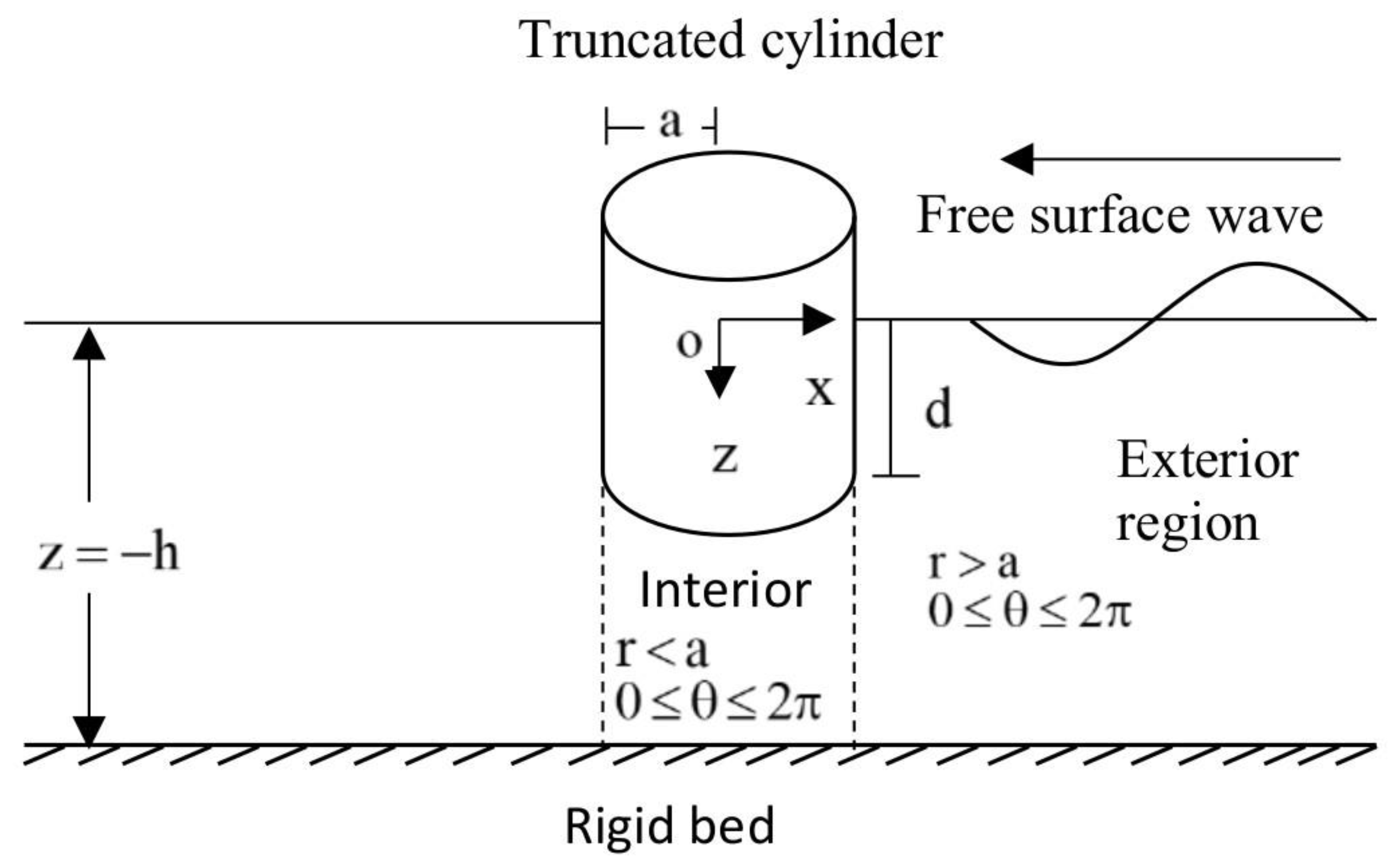
The mathematical formulation of the problem is considered in three-dimensional Cartesian coordinate system (x*, y*, z*), x*–y* being the horizontal plane and z*-being pointing upward starting at the undisturbed free surface. The fluid occupies the region –h* < z* < 0, –∞ < x*< ∞ and a cylinder of radius r = a is floating at z* = 0 with draft d and water depth at z = −h*. * indicates a dimensional variable. Hence, the fluid region is divided into two regions: an interior which corresponds to the area below the cylinder and exterior region constitute the rest of the region (Figure 1). Therefore, the velocity potential and the free surface displacement in the exterior region are denoted by Φ* and η*, respectively. Furthermore, the fluid is assumed to be inviscid, incompressible, and the motion is irrotational, and simple harmonic in time with angular frequency ω.

The velocity potential Φ* satisfy the Laplace equation as:

$${\overline{\nabla }}^2{\Phi }^{*}+{\Phi }_{z^{*}{z}^{*}}^{*}=0\mathrm{for}-h^{*}\le z^{*}\le 0$$

(1)

where $\overline{\nabla }\equiv (\partial /\partial x^{*},\partial /\partial y^{*})$ in Cartesian co-ordinate system, the subscript ‘$z^{*}{z}^{*}$’ denotes the double partial derivatives w.r.t to $z^{*}$.

As the bottom is considered as rigid, the bottom boundary condition yields.

$${\Phi }_{z^{*}}^{*}=0\mathrm{at}{z}^{*}=-h^{*}$$

(2)

The equations of motion for the exterior region can be expressed as:

$$\frac{\partial {\Phi }^{*}}{\partial t^{*}}+\frac{1}{2}{\left(\nabla {\Phi }^{*}\right)}^2+\frac{P}{\rho }+g{z}^{*}=0\mathrm{for}-h^{*}\le z^{*}\le 0,r\ge a$$

(3)

where $P$ is the pressure, g = gravitational constant, and ρ = fluid density. From Equation (3), the pressure continuity at the free surface $z^{*}={\eta }^{*}$ by considering atmospheric pressure zero leads to

$$\frac{\partial {\Phi }^{*}}{\partial t^{*}}+\frac{1}{2}{\left(\nabla {\Phi }^{*}\right)}^2+g{\eta }^{*}=0$$

(4)

Now, the problem is governed by one-linear equations and three boundary conditions which are non-linear in the potential variables ${\Phi }^{*}$ and ${\eta }^{*}$. Therefore, the problem itself is non-linear as ${\eta }^{*}$ is not known a priori.

The next subsection derives the nonlinear BEs for exterior region associated with free surface motions in the presence of floating fixed vertical cylinder.

2.1. Non-Linear Boussinesq Equations (BEs) in the Exterior Region

The following non-dimensional variables are used for the derivation of nonlinear BEs with a floating truncated vertical cylinder (as in [25,26]):

$$\begin{array}{l}x=\frac{x^{*}}{\lambda },\mathrm{y}=\frac{y^{*}}{\lambda },z=\frac{z^{*}}{h_0},t=\frac{t^{*}\sqrt{g{h}_0}}{\lambda },\eta =\frac{{\eta }^{*}}{I_0},\\ h=\frac{h^{*}}{h_0},p=\frac{p^{*}}{\rho g{I}_0},\Phi =\frac{{\Phi }^{*}}{I_0\lambda \sqrt{g{h}_0}},r=\frac{r^{*}}{\lambda },\end{array}$$

(5)

where $h$= length representative of the water depth scaled by $h_0$, $t^{*}$= time, $p^{*}$= water pressure, $\lambda$ is the wave length, $I_0$ is the wave amplitude, ${\eta }^{*}$= free surface elevation, and $r^{*}$= radius of the cylinder.

In order to characterizing long waves, the following two non-dimensional parameters $\epsilon$ and $\mu$ are used as:

$$\epsilon =\frac{I_0}{h_0},\mu =\frac{h_0}{\lambda }$$

(6)

where $\epsilon$ and $\mu$ in Equation (6) are the nonlinearity and frequency dispersion and are assumed to be small.

The non-dimensional three-dimensional governing equation in terms of velocity potential $\Phi$ is expressed as (hereafter all the non-dimensional symbols are neglected):

$${\mu }^2{\overline{\nabla }}^2\Phi +{\Phi }_{zz}=0\mathrm{for}-h\le z\le \epsilon \eta$$

(7)

where ${\overline{\nabla }}^2=\frac{{\partial }^2}{\partial r^2}+\frac{1}{r}\frac{\partial }{\partial r}+\frac{1}{r^2}\frac{\partial }{\partial {\theta }^2}$, with $r$ is the radial distance from the z-axis and $\theta$ is the angle about the x-axis.

The generalized Bernoulli equation read as dynamic boundary condition:

$${\Phi }_t+g\eta +\frac{\epsilon }{2}{\left|\nabla \Phi \right|}^2+\frac{U_r}{2}{\Phi }_z^2=0\mathrm{at}z=\epsilon \eta ,r\ge a$$

(8)

where the subscripts ‘$t$’ and z denote the partial derivative w. r. t. $t$ and z, respectively. $U_r=\epsilon /{\mu }^2$ is known as the Ursell number.

The kinematic condition at $z=\epsilon \eta$ in non-dimensional form is given by:

$${\Phi }_z-{\mu }^2({\eta }_t+\epsilon \overline{\nabla }\Phi \overline{\nabla }\eta )=0\mathrm{at}z=\epsilon \eta ,r\ge a$$

(9)

No flow condition at the bottom boundary yields:

$${\Phi }_z=0\mathrm{at}z=-h$$

(10)

Integrating Equation (7) w. r. t. $z$ and using boundary conditions (9–10), results in:

$$\overline{\nabla }\left[{\displaystyle {\int }_{-h}^{\epsilon \eta }\overline{\nabla }\Phi dz}\right]=-{\eta }_t\mathrm{for}r\ge a$$

(11)

The kinematic boundary condition on the cylinder is given by:

$$\frac{\partial \Phi }{\partial r}=0\mathrm{at}r=a,0<z<d$$

(12)

The velocity potential satisfies the far field radiation condition as

$$\underset{r\to \infty }{\lim }\sqrt{r}\left(\frac{\partial \Phi }{\partial r}+ir\Phi \right)=0$$

(13)

The next section presents the non-linear BEs in terms of velocity potential with depth parameters at specific elevations in the exterior region based on perturbation technique and second-order wave amplitudes around the floating fixed truncated vertical cylinder in the application range of weakly dispersive waves.

2.2. BEs for Exterior Region Based on Perturbation Technique

The velocity potential $\Phi$ in polynomial form can be expanded as:

$$\Phi (x,y,z;t)={\displaystyle \sum _{n=0}^{\infty }{\mu }^{2n}{\Phi }_n(x,y,z;t)}\mathrm{for}r\ge a$$

(14)

where $x=r\cos \theta \mathrm{and}y=r\sin \theta$. Substituting Equation (5) into Equations (7) and (10) equating the powers of $\mu$ in terms of the specific elevation at $z=z_{\alpha }$ $(-h\le z_{\alpha }\le 0)$ and related velocity potential ${\Phi }_{\alpha }$, one can obtain (as in [8,27]).

$$\Phi ={\Phi }_{\alpha }+{\mu }^2[\{\frac{(z_{\alpha }^2-z^2)}{2}{\overline{\nabla }}^2{\Phi }_{\alpha }-(z-z_{\alpha })\overline{\nabla }(h\overline{\nabla }{\Phi }_{\alpha })\}]+o({\mu }^4)\mathrm{for}r\ge a$$

(15)

Again, substituting Equation (15) into Equation (11), and on simplification, the BE in terms of ${\Phi }_{\alpha }$ and $\eta$ in the exterior region is obtained as:

$$\begin{array}{l}{\eta }_t+h{\overline{\nabla }}^2{\Phi }_{\alpha }+{\mu }^2\{\left(\frac{z_{\alpha }^{2}h}{2}+z_{\alpha }{h}^2+\frac{h^3}{3}\right){\overline{\nabla }}^2{\overline{\nabla }}^2{\Phi }_{\alpha }+\left(z_{\alpha }h+\frac{h^2}{2}\right)\overline{\nabla }\overline{\nabla }(\overline{\nabla }{\Phi }_{\alpha }\overline{\nabla }h)\}+\epsilon \overline{\nabla }(\eta \overline{\nabla }{\Phi }_{\alpha })\\ +o({\epsilon }^2{\mu }^2,{\epsilon }^3{\mu }^2,{\mu }^4)=0\mathrm{for}r\ge a.\end{array}$$

(16)

Substituting $\Phi$ from Equation (15) into Equation (8), the nonlinear free surface condition is derived as:

$$\begin{array}{l}-\eta +{\Phi }_{\alpha t}+{\mu }^2\left(\frac{z_{\alpha }^2}{2}+h{z}_{\alpha }\right){\overline{\nabla }}^2{\Phi }_{\alpha t}+\frac{\epsilon }{2}{(\overline{\nabla }{\Phi }_{\alpha })}^2+\frac{U_r}{2}{\Phi }_{\alpha z}^2+o({\epsilon }^2,\epsilon {\mu }^2,{\mu }^4)=0\\ \mathrm{for}r\ge a\end{array}$$

(17)

where the higher-order non-linear terms are neglected.

The next subsection presents the second-order free surface elevations and velocity potentials in the exterior and interior regions using suitable Bessel’s and Hankel’s functions associated with wave diffraction by a floating fixed truncated vertical cylinder.

2.3. Second-Order Free Surface Wave and Velocity Potentials for Exterior and Interior Region

The second-order free surface displacement in exterior region $r\ge a$ can be expressed as:

$${\eta }_{mn}^{\pm }={\displaystyle \sum _{l=0}^{\infty }{A}_{mn}^{\pm }{J}_l(k_{mn}^{\pm }r)\cos (k_{mn}^{\pm }x+{\omega }_{mn}^{\pm }t+{\phi }_{mn}^{\pm })}$$

(18)

where $A_{mn}^{\pm }$ are the unknown second-order wave amplitude to be determined. Further, the + sign and – sign denote the super- and sub-harmonic parts generated by the interactions of the linear waves (m-wave and n-wave), respectively, $J_l(k_{mn}^{\pm }r)$ is the Bessel function of first kind of order l (as in [3]), $k_{mn}^{\pm }=k_m\pm k_n$, ${\omega }_{mn}^{\pm }={\omega }_m\pm {\omega }_n$, and ${\phi }_{mn}^{\pm }={\phi }_m\pm {\phi }_n$ with k_m and k_n are the wave numbers of the m and n-waves associated with the wave frequency ${\omega }_m$ and ${\omega }_n$, respectively. Further, ${\phi }_m$ and ${\phi }_n$ are the phases of m- and n-wave, respectively.

The incident velocity potential ${\Phi }_{\alpha mn}^{inc}$ and the diffracted velocity potential ${\Phi }_{\alpha mn}^{dif}$ can be expanded as:

$${\Phi }_{\alpha mn}^{inc}={\displaystyle \sum _{l=0}^{\infty }{B}_{mn}^{\pm }}{J}_l(k_{mn}^{\pm }r)\sin (k_{mn}^{\pm }x+{\omega }_{mn}^{\pm }t+{\phi }_{mn}^{\pm })\mathrm{for}r\ge a$$

(19)

$${\Phi }_{\alpha mn}^{dif}={\displaystyle \sum _{l=0}^{\infty }{C}_{mn}^{\pm }}{H}_l(k_{mn}^{\pm }r)\sin (k_{mn}^{\pm }x+{\omega }_{mn}^{\pm }t+{\phi }_{mn}^{\pm })\mathrm{for}r\ge a$$

(20)

where $H_l(k_{mn}^{\pm }r)$ is the Hankel function of first kind of order l. $B_{mn}^{\pm }$ and $C_{mn}^{\pm }$ are the unknown coefficients of super- and sub-harmonic waves.

Hence, using Equations (19) and (20), the total potential ${\Phi }_{\alpha mn}^{ext}$ can be expressed as:

$$\begin{array}{l}{\Phi }_{\alpha mn}^{ext}={\Phi }_{\alpha mn}^{inc}+{\Phi }_{\alpha mn}^{dif}={\displaystyle \sum _{l=0}^{\infty }\{B_{mn}^{\pm }}{J}_l(k_{mn}^{\pm }r)+C_{mn}^{\pm }{H}_l(k_{mn}^{\pm }r)\}\times \sin (k_{mn}^{\pm }x+{\omega }_{mn}^{\pm }t+{\phi }_{mn}^{\pm })\\ \mathrm{for}r\ge a\end{array}$$

(21)

The second-order velocity potential ${\Phi }_{\alpha mn}^{\mathrm{int}}$ in the interior region can be written as:

$${\Phi }_{\alpha mn}^{\mathrm{int}}={\displaystyle \sum _{l=0}^{\infty }{D}_{mn}^{\pm }}{I}_l(k_{mn}^{\pm }r)\sin \left(k_{mn}^{\pm }x+{\omega }_{mn}^{\pm }t+{\phi }_{mn}^{\pm }\right)\mathrm{for}r\le a$$

(22)

where $D_{mn}^{\pm }$ is the unknown coefficient and $I_l(k_{mn}^{\pm }r)$ are the modified Bessel functions of first kind of order l.

The next subsection determines the unknown coefficients in terms of second-order super- and sub-harmonic amplitudes associated with free surface elevations and velocity potentials using matching conditions.

2.4. Determination of Second-Order Free Surface Amplitude and Unknown Coefficients

The unknowns $A_{mn}^{\pm }$, $B_{mn}^{\pm }$, $C_{mn}^{\pm }$ and $D_{mn}^{\pm }$ associated with Equations (18)–(20) and Equation (22) can be determined by applying the structural boundary conditions and matching the pressure and normal velocities across the boundary at r = a. The boundary conditions are given by:

$${\frac{\partial {\varphi }_{\alpha mn}^{ext}}{\partial r}|}_{r=a}=0\mathrm{for}0\le z\le d,$$

(23)

$${{\varphi }_{\alpha mn}^{ext}|}_{r=a}={{\varphi }_{\alpha mn}^{int}|}_{r=a}\mathrm{for}d\le z\le h,$$

(24)

$${\frac{\partial {\varphi }_{\alpha mn}^{ext}}{\partial r}|}_{r=a}={\frac{\partial {\varphi }_{\alpha mn}^{int}}{\partial r}|}_{r=a}\mathrm{for}d\le z\le h$$

(25)

The wave amplitudes $A_{mn}^{\pm }$ defined in Equation (18) can be determined by applying the structural boundary condition (23) and using Equation (18) into Equation (15). However, hereafter the super-harmonic wave amplitude is considered for comparing with CFD model simulations and the effect of sub-harmonic second-order wave amplitudes on different parametric values in subsequent sections.

Applying the boundary condition (24) into Equation (21) and Equation (22), one can obtain

$${\displaystyle \sum _{l=0}^{\infty }{B}_{mn}^{\pm }\left\{J_l(k_{mn}^{\pm }a)S_{mn}^{\pm }+{\mu }^{2}Z{P}_{mn}^{\pm }\right\}}+{\displaystyle \sum _{l=0}^{\infty }{C}_{mn}^{\pm }\left\{H_l(k_{mn}^{\pm }a)S_{mn}^{\pm }+{\mu }^{2}Z{Q}_{mn}^{\pm }\right\}}={\displaystyle \sum _{l=0}^{\infty }{D}_{mn}^{\pm }}{I}_l(k_{mn}^{\pm }a)S_{mn}^{\pm }$$

(26)

where:

$$\begin{array}{l}Z=(z_{\alpha }^2-z^2)/2-(z-z_{\alpha })h,\\ S_{mn}^{\pm }=\sin (k_{mn}^{\pm }a(\cos \theta )+\omega t),\end{array}$$

$$\begin{array}{l}{P}_{mn}^{\pm }=H_l^{\prime }(k_{mn}^{\pm }a)(k_{mn}^{\pm }a)+(1/2)k_{mn}^{\pm }{H}_l^{\prime }(k_{mn}^{\pm }a)\{k_{mn}^{\pm }a\cos (2\theta )-k_{mn}^{\pm }a{\sin }^2(\theta )\}{S}_{mn}^{\pm },\\ Q_{mn}^{\pm }=\{(-1/a)H_l^{″}(k_{mn}^{\pm }a)(k_{mn}^{\pm }{\cos }^2\theta )+(1/a^2)H_l^{\prime }(k_{mn}^{\pm }a)\}\\ \hspace{1em}\hspace{1em}\hspace{1em}\times \{(1/4){(k_{mn}^{\pm }a)}^2\sin (2\theta )-\cos \theta \}{S}_{mn}^{\pm }.\end{array}$$

Furthermore, using Equation (21) into the boundary condition (23), one can obtain

$$\begin{array}{l}{\displaystyle \sum _{l=0}^{\infty }{B}_{mn}^{\pm }}\left[\{J_l^{\prime }(k_{mn}^{\pm }a)+{\mu }^{2}Z{U}_{1mn}^{\pm }\}{S}_{mn}^{\pm }+\{J_l(k_{mn}^{\pm }a)(k_{mn}^{\pm }\cos \theta )+{\mu }^{2}Z{V}_{1mn}^{\pm }\}{U}_{mn}^{\pm }\right]\\ +{\displaystyle \sum _{l=0}^{\infty }{C}_{mn}^{\pm }}\left[\{H_l^{\prime }(k_{mn}^{\pm }a)+{\mu }^{2}Z{P}_{1mn}^{\pm }\}{S}_{mn}^{\pm }+\{H_l(k_{mn}^{\pm }a)(k_{mn}^{\pm }\cos \theta )+{\mu }^{2}Z{Q}_{1mn}^{\pm }\}{U}_{mn}^{\pm }\right]=0\end{array}$$

(27)

where

$$\begin{array}{l}{U}_{mn}^{\pm }=\cos (k_{mn}^{\pm }a(\cos \theta )+\omega t),\\ P_{1mn}^{\pm }=\{H_l^{‴}(k_{mn}^{\pm }a)(k_{mn}^{\pm }\cos \theta )+(1/a^2)H_l^{\prime }(k_{mn}^{\pm }a)k_{mn}^{\pm }\}\times \{k_{mn}^{\pm }a\cos (2\theta )-k_{mn}^{\pm }a{\sin }^2(\theta )\},\\ Q_{1mn}^{\pm }=\{(-1/a)H_l^{″}(k_{mn}^{\pm }a)(k_{mn}^{\pm }{\cos }^2\theta )+(1/a^2)H_l^{\prime }(k_{mn}^{\pm }a)\}\times \{(1/4){(k_{mn}^{\pm }a)}^2\sin (2\theta )-\cos \theta \},\\ U_{1mn}^{\pm }=\{J_l^{‴}(k_{mn}^{\pm }a)(k_{mn}^{\pm }\cos \theta )+(1/a^2)J_l^{\prime }(k_{mn}^{\pm }a)k_{mn}^{\pm }a\}\times \{k_{mn}^{\pm }a\cos (2\theta )-k_{mn}^{\pm }a{\sin }^2(\theta )\},\\ V_{1mn}^{\pm }=\{(-1/a)J_l^{″}(k_{mn}^{\pm }a)(k_{mn}^{\pm }{\cos }^2\theta )+(1/a^2)J_l^{\prime }(k_{mn}^{\pm }a)\}\times \{(-1/4){(k_{mn}^{\pm }a)}^2\sin (2\theta )-\cos \theta \}.\end{array}$$

Furthermore, the velocity continuity condition (25) gives

$$\begin{array}{l}{\displaystyle \sum _{l=0}^{\infty }{B}_{mn}^{\pm }}\left[\{J_l^{\prime }(k_{mn}^{\pm }a)S_{mn}^{\pm }+J_l(k_{mn}^{\pm }a)k_{mn}^{\pm }\cos \theta U_{mn}^{\pm }\right]\\ +{\displaystyle \sum _{l=0}^{\infty }{C}_{mn}^{\pm }}\left[\{H_l^{\prime }(k_{mn}^{\pm }a)S_{mn}^{\pm }+H_l(k_{mn}^{\pm }a)(k_{mn}^{\pm }\cos \theta )U_{mn}^{\pm }\right]\\ +{\displaystyle \sum _{l=0}^{\infty }[{\mu }^2\{(z_{\alpha }^2-z^2)/2{\overline{\nabla }}^2\frac{\partial }{\partial r}({\Phi }_{\alpha mn}^{ext})-(z-z_{\alpha })(\overline{\nabla }h)\overline{\nabla }\frac{\partial }{\partial r}({\Phi }_{\alpha mn}^{ext})\}}]\\ ={\displaystyle \sum _{l=0}^{\infty }{D}_{mn}^{\pm }}\{I_l^{\prime }(k_{mn}^{\pm }a)S_{mn}^{\pm }+I_l(k_{mn}^{\pm }a)k_{mn}^{\pm }\cos \theta U_{mn}^{\pm }\}.\end{array}$$

(28)

Further, applying the structural boundary condition (23) and using Equation (18) into Equation (17), one can obtain the second-order wave amplitude $A_{mn}^{\pm }$ as

$$A_{mn}^{\pm }=C_{mn}^{\pm }\left[\{H_l(k_{mn}^{\pm }a){\omega }_{mn}^{\pm }{U}_{mn}^{\pm }+{\mu }^2\{(z_{\alpha }^2/2)+h{z}_{\alpha }\}{H}_l(k_{mn}^{\pm }a)U_{mn}^{\pm }\}-L_{mn}^{\pm }\right]/J_l(k_{mn}^{\pm }a)U_{mn}^{\pm }$$

(29)

Now solving Equations (26)–(28), the second-order wave amplitude $D_{mn}^{\pm }$ is obtained as

$$D_{mn}^{\pm }=C_{mn}^{\pm }\left[\{H_l(k_{mn}^{\pm }a)S_{mn}^{\pm }+{\mu }^{2}Z{Q}_{mn}^{\pm }\}-G_{mn}^{\pm }\{J_l(k_{mn}^{\pm }a)S_{mn}^{\pm }+{\mu }^{2}Z{P}_{mn}^{\pm }\}\right]/I_l(k_{mn}^{\pm }a)S_{mn}^{\pm }$$

(30)

where

$$\begin{array}{cc}\hfill L_{mn}^{\pm }=& W_{mn}^{\pm }{X}_{mn}^{\pm }+J_l(k_{mn}^{\pm }a){\omega }_{mn}^{\pm }{U}_{2mn}^{\pm }{\mu }^{2}Z(P_{mn}^{\pm }+Q_{mn}^{\pm })\hfill \\ & /\{J_l^{\prime }(k_{mn}^{\pm }a)+{\mu }^{2}Z{U}_{2mn}^{\pm }\}{S}_{mn}^{\pm }+\{J_l(k_{mn}^{\pm }a)k_{mn}^{\pm }\cos \theta +{\mu }^{2}Z{V}_{2mn}^{\pm }\}{U}_{2mn}^{\pm }\hfill \end{array}$$

$$\begin{array}{cc}\hfill G_{mn}^{\pm }=& \left[\{H_l^{\prime }(k_{mn}^{\pm }a)+{\mu }^{2}Z{P}_{1mn}^{\pm }+\}{S}_{mn}^{\pm }+\{H_l(k_{mn}^{\pm }a)k_{mn}^{\pm }\cos \theta +{\mu }^{2}Z{Q}_{1mn}^{\pm }\}{U}_{mn}^{\pm }\right]\hfill \\ & \hfill /\left[\{J_l^{\prime }(k_{mn}^{\pm }a)+{\mu }^{2}Z{U}_{1mn}^{\pm }+\}{S}_{mn}^{\pm }+\{J_l(k_{mn}^{\pm }a)k_{mn}^{\pm }\cos \theta +{\mu }^{2}Z{V}_{1mn}^{\pm }\}{U}_{mn}^{\pm }\right]\end{array}$$

with

$$U_{mn}^{\pm }=\{J_l^{‴}(k_{mn}^{\pm }a)k_{mn}^{\pm }\cos \theta +(1/a^2)J_l^{‴}(k_{mn}^{\pm }a)(k_{mn}^{\pm }a)\}\times \{k_{mn}^{\pm }a\cos (2\theta )-k_{mn}^{\pm }a{\sin }^2\theta \},$$

$$V_{2mn}^{\pm }=\{(-1/a)J_l^{″}(k_{mn}^{\pm }a){(k_{mn}^{\pm }\cos \theta )}^2+(1/a^2)J_l^{\prime }(k_{mn}^{\pm }a)(k_{mn}^{\pm })\}\times \{(-1/4)\sin (2\theta ){(k_{mn}^{\pm }a)}^2-\cos \theta \},$$

$$W_{mn}^{\pm }=J_l(k_{mn}^{\pm }a){\omega }_{mn}^{\pm }{U}_{mn}^{\pm }+{\mu }^2\{(z_{\alpha }^2/2)+h{z}_{\alpha }\}{J}_l(k_{mn}^{\pm }a)S_{mn}^{\pm },$$

$$X_{mn}^{\pm }=\{H_l^{\prime }(k_{mn}^{\pm }a)S_{mn}^{\pm }+H_l(k_{mn}^{\pm }a)k_{mn}^{\pm }\cos \theta U_{mn}^{\pm })$$

where $H_l^{\prime }$, $H_l^{″}$ and $H_l^{‴}$ denote to the 1st, 2nd, and 3rd derivatives of Hankel’s function, respectively, and the same as with Bessel’s function $J_l$.

The next section describes the numerical CFD model based on OpenFOAM solver in terms of CFD, mathematical model equations, computational mesh, the case set up, and computational resource associated with the aforementioned problem.

3. Computational Fluid Dynamics (CFD) Model

3.1. Brief Description of CFD Model

For CFD simulations in the study, the open source CFD tooklit OpenFOAM (Open Source Field Operation and Manipulation) was used. A relatively old version of OpenFOAM ws used (version 2.4.0), coupled with waves2Foam utility for wave generation. A detailed description on the CFD solver can be found at works by Jasak [28].

OpenFOAM is governed by the Navier–Stokes and continuity equation, and models an incompressible laminar flow of a Newtonian fluid. The Navier–Stokes equation is given by:

$$\rho \left(\frac{\partial v}{\partial t}+U\nabla U\right)=-\nabla p+\mu {\nabla }^{2}U+\rho g$$

(31)

where $U$ is the velocity, $p$ is the pressure, $\mu$ is the dynamic viscosity, $g$ is acceleration due to gravity, and ${\nabla }^2$ is the Laplace operator. Furthermore, the continuity equation is of the form:

$$\nabla U$$

(32)

The governing equations are discretized using the Finite Volume Method (FVM). Further special and temporal discretization are performed using second and first order methods. Pressure velocity coupling is done using the PISO-SIMPLE (PIMPLE) algorithm. The solver follows the Cartesian coordinate system. The volume of fluid (VoF) method together with the artificial compression technique tracks the free surface elevation, using the volume fraction technique. The equation for the volume fraction is obtained as

$$\frac{\partial \alpha }{\partial t}+\nabla (\alpha U)$$

(33)

where $U$ is the velocity field, $\alpha$ is the volume fraction of water in the cell and varies from 0 to 1, representing full of air to full of water, respectively.

OpenFOAM incorporates several two-equation turbulence models for turbulence modelling and also has incorporated a wall function model. For this study, kOmegaSST turbulence model was used, and the waves were generated following Stokes second-order wave theory.

3.2. Computational Mesh

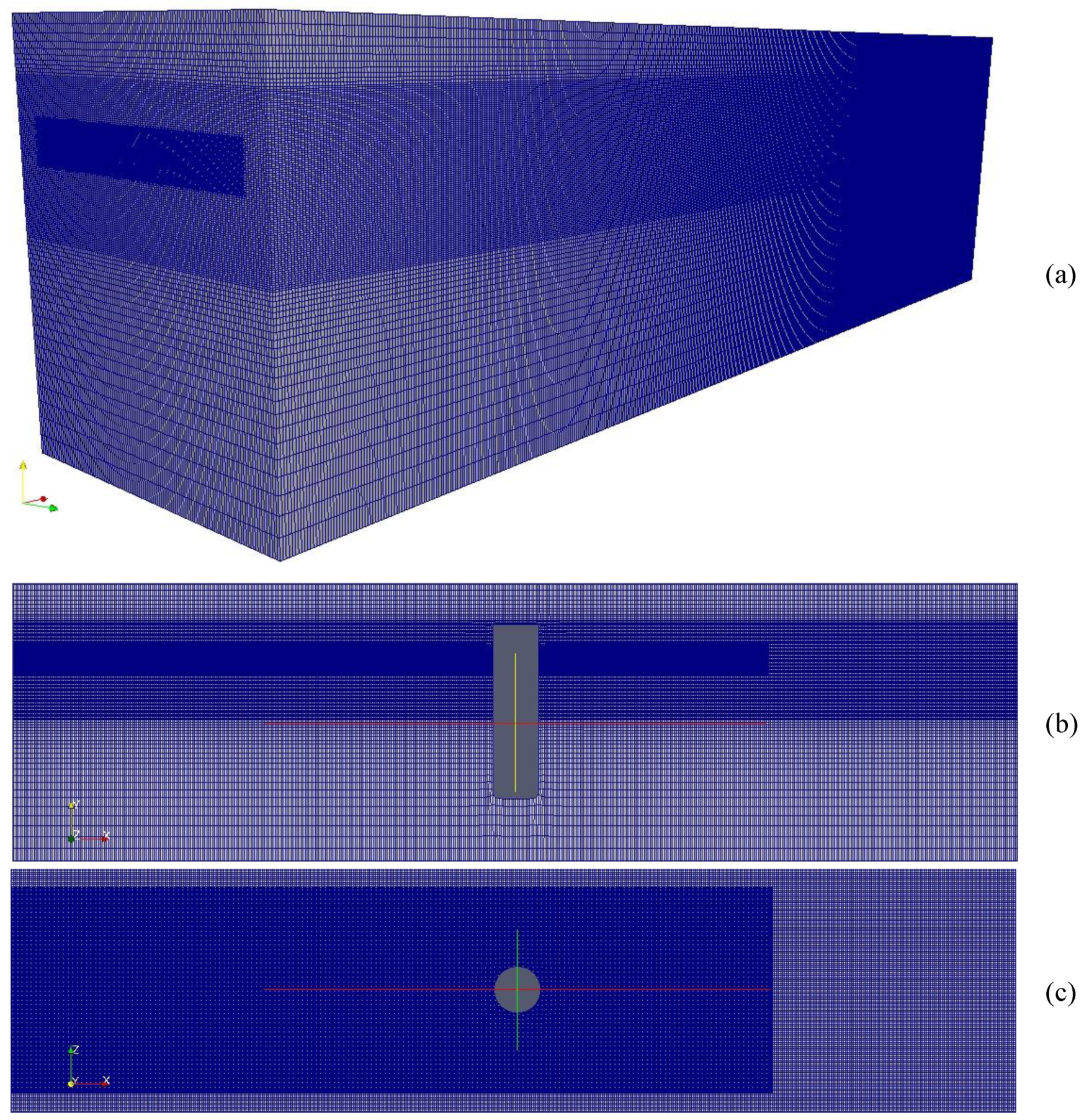
For mesh generation for the case, the OpenFOAM mesh generation utility was used. Depending on the settings, the utility generates hybrid mesh that incorporates both structures and unstructured mesh for an efficient solution. Initially, blockMesh utility is used to generate the rectangular simulation domain using hexahedral mesh. In the mesh, y ‘ + ve’ represents vertical positive direction, and the horizontal free surface is in the x–z plane. The domain was further refined using toposet and refinmesh commands in specific locations, near the geometry and free surface, for better flow prediction around the geometry and better propagation of waves. Finally, the cylinder geometry was integrated to the domain using the snappyHexMesh utility, no refinement or mesh layer was applied in snappyHexMesh.

Two different mesh resolutions were used for simulating the cases to ensure that the mesh satisfies the minimum number of cell requirements per wave height and wave length, while consuming minimum resources. The domain lengths and depths were also varied for the various cases to ensure enough space for the wave relaxation zone and propagation zone, and to maintain a relatively shallow water case for comparing the results with the Boussinesq model. Mesh resolution was maintained such that for the smallest wave length and wave height case, there were 77 cells per wave length and 8 cells per wave height. However, this was the configuration for the shortest wave length and wave height, and the later waves had more cells per wave length and height. For the first five cases, a cell spacing of 0.01 in the X and Z direction was used, and for Y it was 0.005. For the rest of the cases, the cell spacing was 0.05 for the X and Z direction and 0.025 for Y. An average mesh resolution of 6 million cells (mostly hexahedral) was used for the cases. The mesh setup for the first cases is shown in Figure 2. As for the later cases (with longer wave lengths), the refinement was confined to the near cylinder area, where wave probes have been placed, instead of the entire wave propagation area. Since the meshes were generated following standard guidelines for wave simulation, an independent grid dependency study was not performed. Nevertheless, the authors’ previous experience from wave simulations indicate that the mesh resolution and distribution used is sufficient to produce reliable results.

3.3. Case Setup

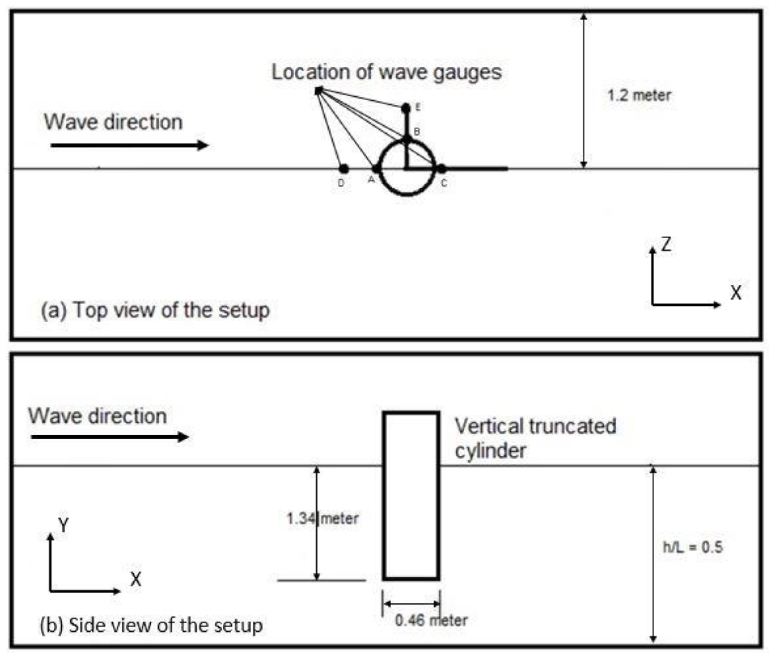
The CFD simulations were performed following the case experimental setup by Mercier and Niedzwecki [25]. Few changes were added to the setup, and all simulations depths were adjusted to maintain a water depth to wavelength ratio (h/L) of 0.5 (water depth/wavelength). This was done to ensure comparability with weakly dispersive Boussinesq model results. Furthermore, considering the relatively small diameter of the cylinder (0.23 m), the domain in lateral direction was reduced from 2.8 m to 1.5 m. The domain length was also adjusted depending on applied wave lengths to ensure enough propagation and dissipation area (at the end of domain) for the incoming waves. On average, the domain length was 12 m.

Following the experimental setup, five wave elevation probes were placed in the simulation domain, three near the cylinder wall and two at a distance, to capture the free surface elevation. The wave probes are denoted by A, B, C, D and E. The locations of the probes are provided in

Table 1. Location of probes in the simulation domain.

Probe	A	B	C	D	E
X (m)	−0.235	0.0	0.235	−0.48	0.0
Y (m)	0.0	−0.235	0.0	0.0	0.48

. The locations of the probes/gauges near the cylinder were slightly modified to place them at the first cell after the cylinder in order to avoid numerical exception. The displacements were at the fraction of millimeters, so it should not impact the simulation outcome. A general arrangement of the experimental setup and simulation domain are shown in Figure 3 and Figure 4, respectively.

All CFD simulations were performed in a desktop machine with Intel^® core i7-7700 CPU with 3.60 GHz processor and 32 GB of RAM. The data was written on an solid state drive (SSD)disk. On average, each case was run for roughly 100 s (simulation time) to ensure around 10 wave encounters and the physical time took to run each case was roughly 75 h.

In the context of the present paper, the 3D numerical simulations were performed for the comparison of results with other methods like experimental data, immersed boundary method (IBM), numerical wave tank (NS) and the present developed BM. The comparison should provide a relative idea about the efficiency and limitations of the methods and models. Therefore, the results obtained from the present BMs and CFD simulations and different method results available in the literature are presented in the subsequent subsections.

4. Numerical Results

In this section, several numerical results associated with the comparison among CFD, experimental, numerical data, and analytical BM results, wave forces, moment, pressure distribution around the cylinder, effects of radius, wave number, water depth, and depth parameters at specific elevations are analyzed. First, comparisons are made of normalized free surface elevations/wave heights among CFD, EFD, and numerical data available in the literature in the probe locations mentioned in the subsequent subsection. Then, the simulation results of wave forces and moments acting on the cylinder and pressure distribution around the vertical cylinder are presented. To check the accuracy of the second-order super-harmonic wave amplitude Boussinesq results, comparisons between the Boussinesq and CFD model simulations on the second-order super-harmonic wave amplitudes for the same probe locations are presented. Finally, to analyze the effects of radius, wave number, water depth, and depth parameters at specific elevations on the second-order sub-harmonic wave amplitudes have been studied.

4.1. Comparison and CFD Simulations

Validation studies for CFD simulation results were undertaken for cases performed in [5,29]. Nine cases were simulated, for different wave lengths and wave heights. The test cases are shown in

Table 2. Specifications for the simulation cases.

Case	Period	Wave Length	Wave Height	Wave Number
number	T (s)	λ (m)	H (m)	k
1	0.70	0.77	0.04	8.21
2	0.87	1.18	0.06	5.32
3	1.00	1.56	0.08	4.02
4	1.12	1.96	0.08	3.21
5	1.40	3.06	0.14	2.05
6	1.70	4.51	0.20	1.39
7	2.00	6.25	0.30	1.01
8	2.22	7.69	0.37	0.82
9	2.50	9.76	0.46	0.64

.

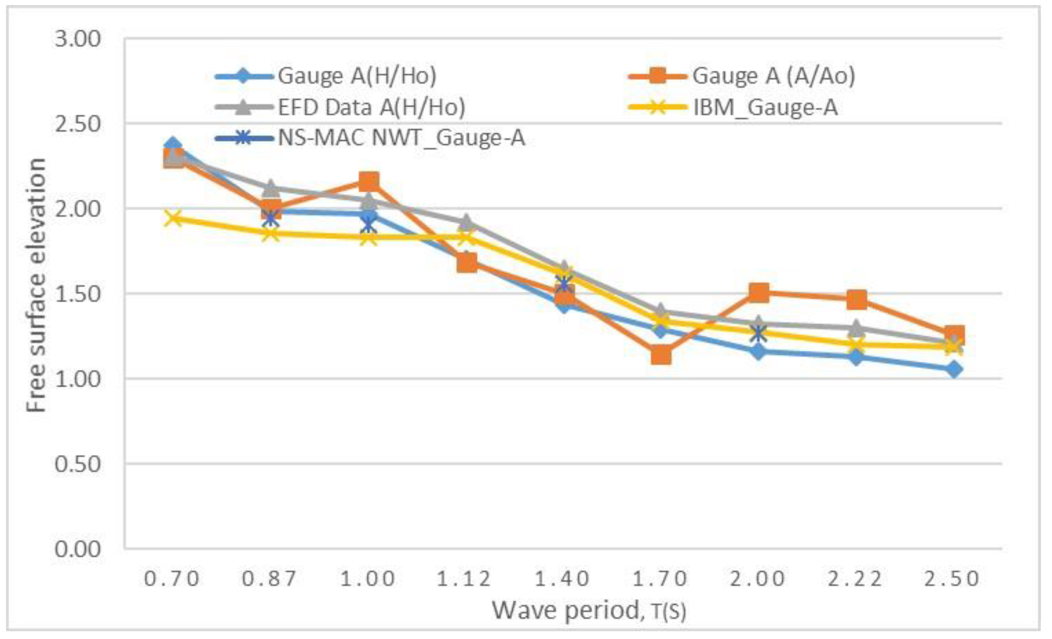
For validation, the simulation results were compared with EFD reported in [28], IBM data reported [5], and numerical wave tank (NWT) data generated using Navier–Stokes (NS) and marker and cell (MAC) methods reported in [30]. For normalization of the free surface elevation data from CFD, the total free surface displacement was divided by the incoming wave height, H/H₀. Calculations were also made based on amplitude since the analytical Boussinesq method calculated the free surface displacement based on amplitude, A/A₀. The target of the simulations was to analyze the diffraction of the incoming waves due to interaction with a floating fixed vertical truncated cylinder. Thus, three wave probes were placed at locations close to the cylinder body, one at 0.48 m before the cylinder and one at 0.48 m at the side (Figure 3).

Figure 5 shows the normalized free surface elevation just before the cylinder at location A. The results show that almost for all cases, the free surface shows higher elevation than the incoming incident waves. Especially for the low wave period cases, the waves surge up to 2.4 times of initial wave height on the cylinder wall. The CFD results here show reasonable agreement with experimental data, although the values do not exactly agree, the trend is well captured. For almost all cases, CFD under predicts the results compared to EFD results. Slight deviation might be explained to some extent by the location of the probe in the CFD model. In CFD, the probe was set 5 mm away from the cylinder, whereas in experiments it was exactly on the cylinder. This could not be done in the CFD model since probes in simulation can only capture data from a cell, not at voids. Furthermore, the numerical dissipation also contributes to the under prediction. The presented CFD results also agree better with the NS model results, since both follow a similar mathematical model, compared to the immersed boundary method results.

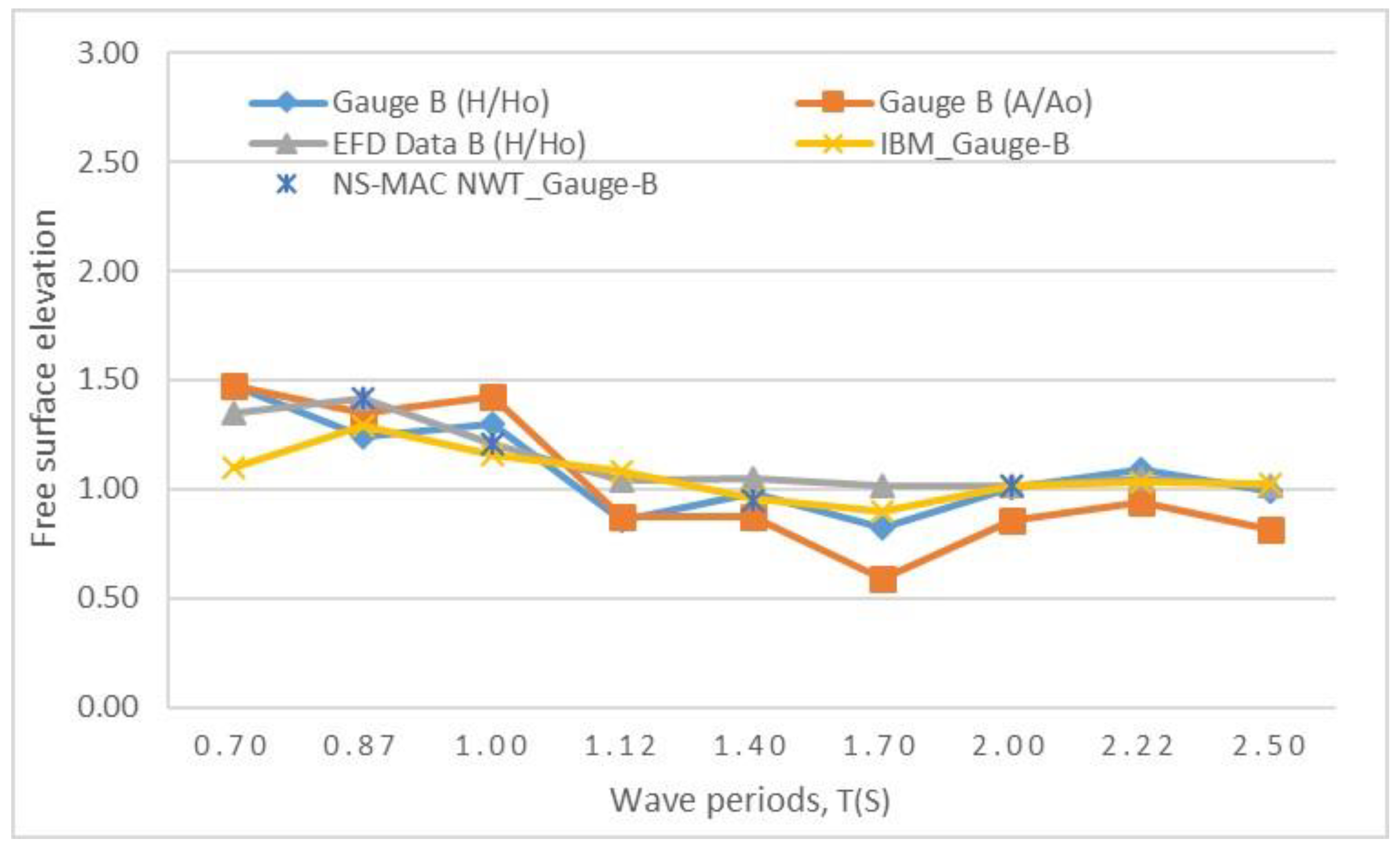
Figure 6 shows surface elevation at the side of the cylinder, at location B. The results show that only for short wave length cases, the incident wave becomes distorted at the side; however, for relatively longer wave lengths, the incident wave height remains almost unchanged. The CFD results here capture the resulting trend, however, they show oscillatory predictions around the EFD data, that is, some cases are over predicted and others are under predicted. Nevertheless, the overall deviation is minimum. Also, for these cases, CFD shows better agreement than the NS model.

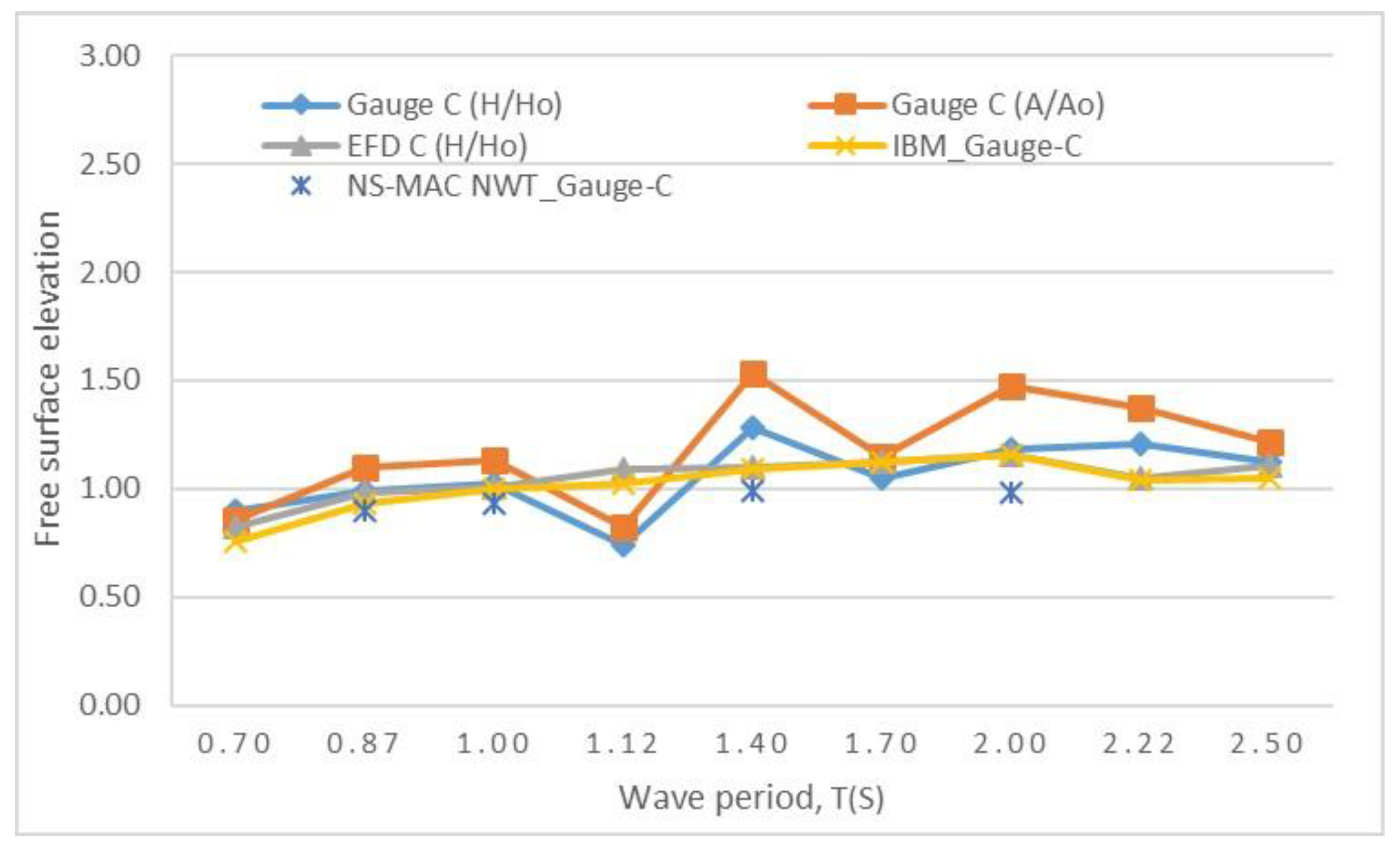
Figure 7 gives free surface elevation just behind the cylinder (location C). It is observed that the diffraction effect is minimum behind the cylinder and the simulations results here capture the trend well, with relatively notable deviation for three cases. For short wavelengths, the waves lose amplitude while interacting with the cylinder and thus show a lower steepness behind the cylinder. As the wave period and height increases, the loss in steepness decreases and the waves end up gaining slight amplitude due to the interaction with the cylinder. However, none of the amplitude gains actually represent a gain in energy, rather just a sudden transfer of energy.

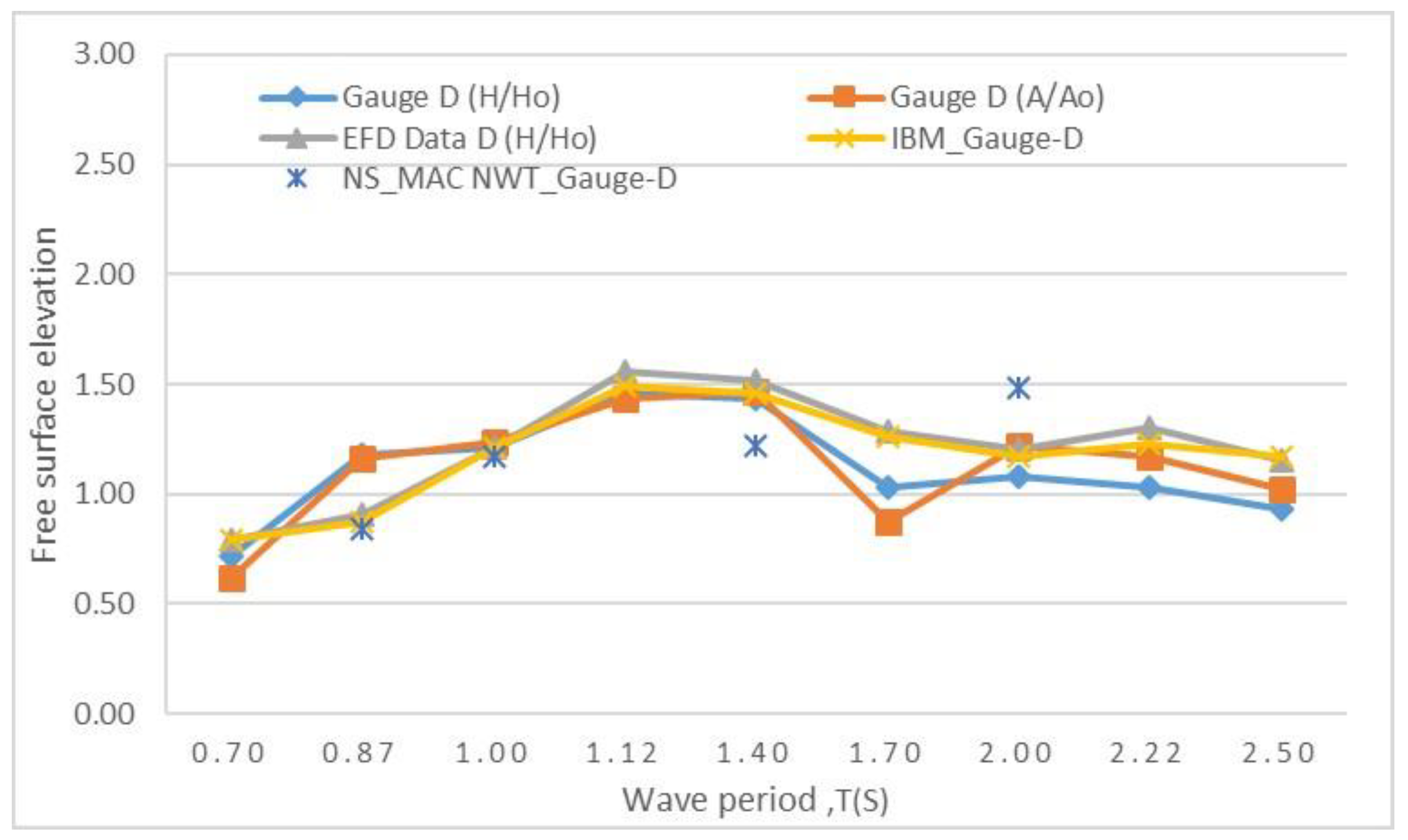
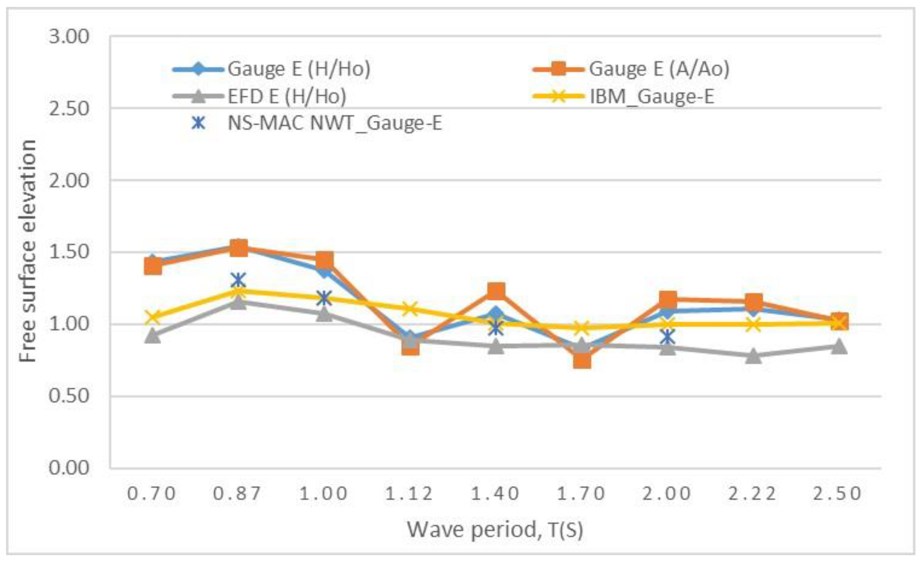
In Figure 8 and Figure 9, the comparison between CFD, experimental, and numerical data in location D and E are shown, which represent free surface elevation at 0.48 m before and at the side of the cylinder. The results show that the effect of the wave and structure interaction can also be observed at roughly one radial distance from the cylinder. As before, the CFD results capture the trend well, with deviation in the values for several cases.

Especially, in case of Figure 9 (position E), the CFD values show relatively high deviation from experimental values, except for three cases. The reason for this over prediction may partly be explained by the relatively short width of the domain in the sides. Because of the slight reflection of the waves by the symmetry planes, the elevations might have been over predicted. Increasing the domain size in the lateral direction might have improved the prediction, however, considering the added computational expense, it was avoided.

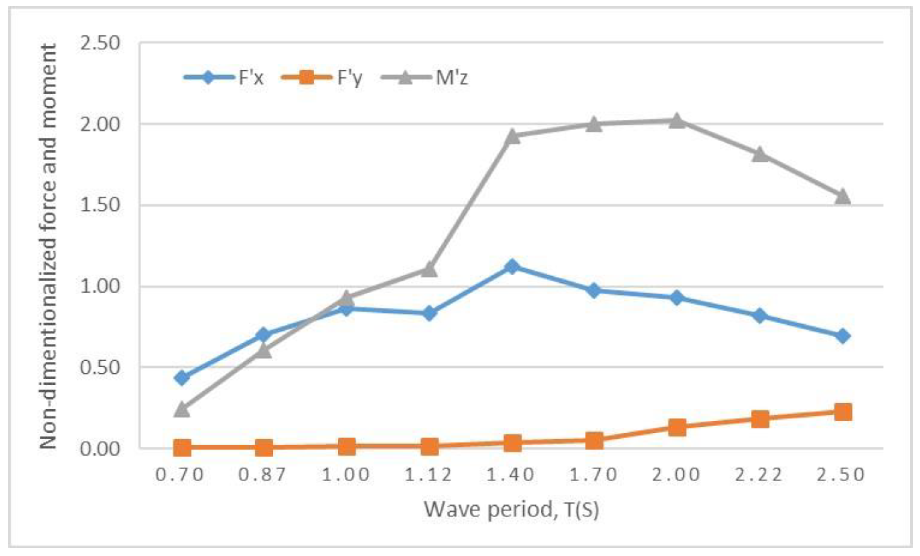
Next, horizontal and vertical forces and pitch moment acting on the cylinder were computed from the simulation results. For non-dimensionalization of the results, the following equations were used.

$$F_x^{\prime }=\frac{F_x}{\rho grT{H}^{\prime }},$$

(34)

$$F_y^{\prime }=\frac{F_y}{\rho grT{H}^{\prime }},$$

(35)

$$M_z^{\prime }=\frac{M_z}{\rho g{r}^{2}T{H}^{\prime }},$$

(36)

where F_x, F_y and M_z represent horizontal and vertical force and pitch moment, respectively, $\rho$ is the fluid density, g is gravitational acceleration, $r$ is the cylinder radius, T is the cylinder draft and H is the incident wave height.

In Figure 10, the horizontal force, vertical force, and moment acting on the cylinder versus wave period are plotted. It is observed that both the horizontal force and pitch moment show similar response with peak amplitude being observed close to the 1.70 wave period. The force and moment decrease for relatively low and high frequency range. Whereas, for the heaving force, it keeps on increasing with the increasing wave period and wave height. This might be because the structure is fixed and is not free to heave with incoming incident waves. With heave-free motion, the results might be slightly different.

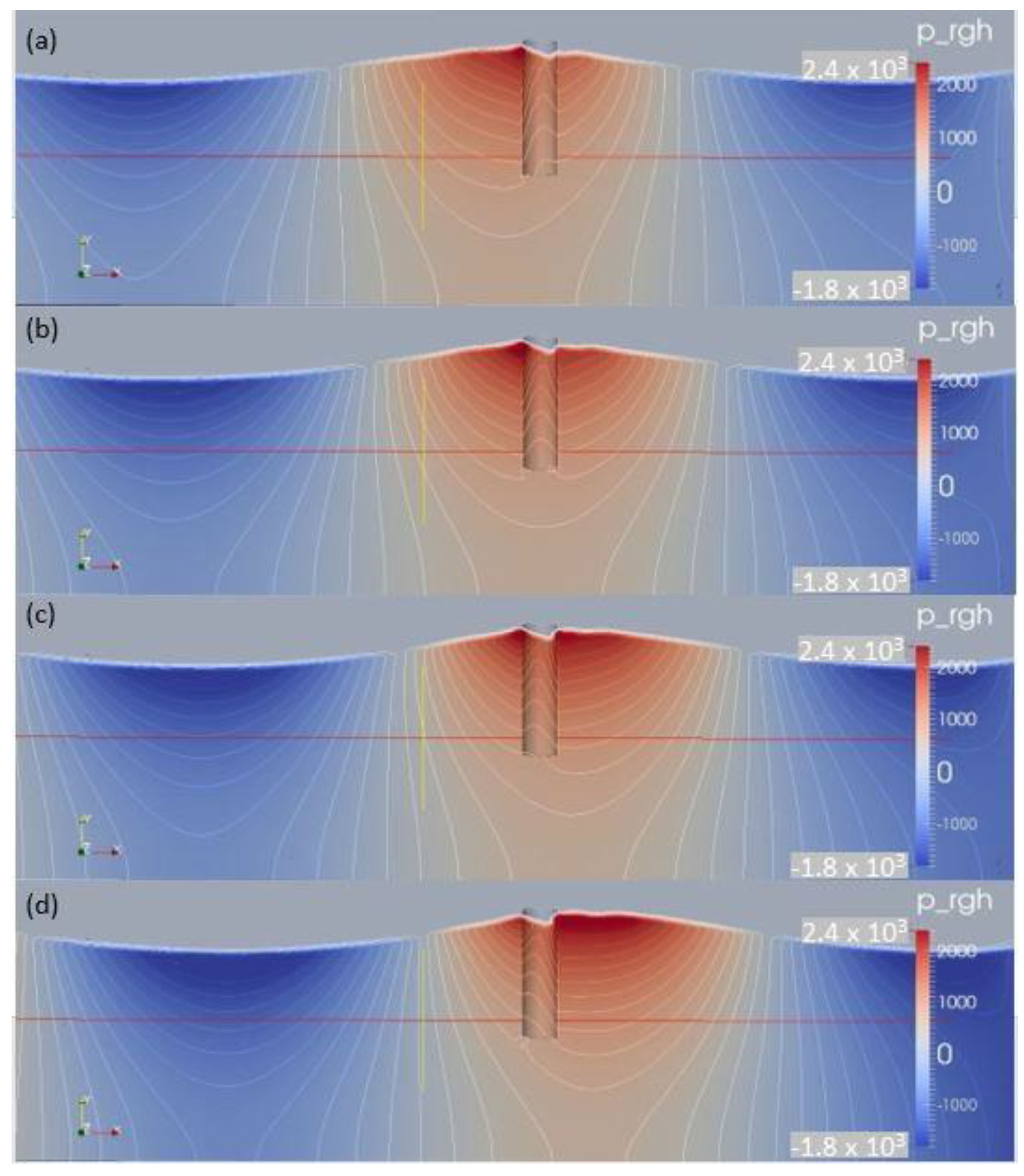
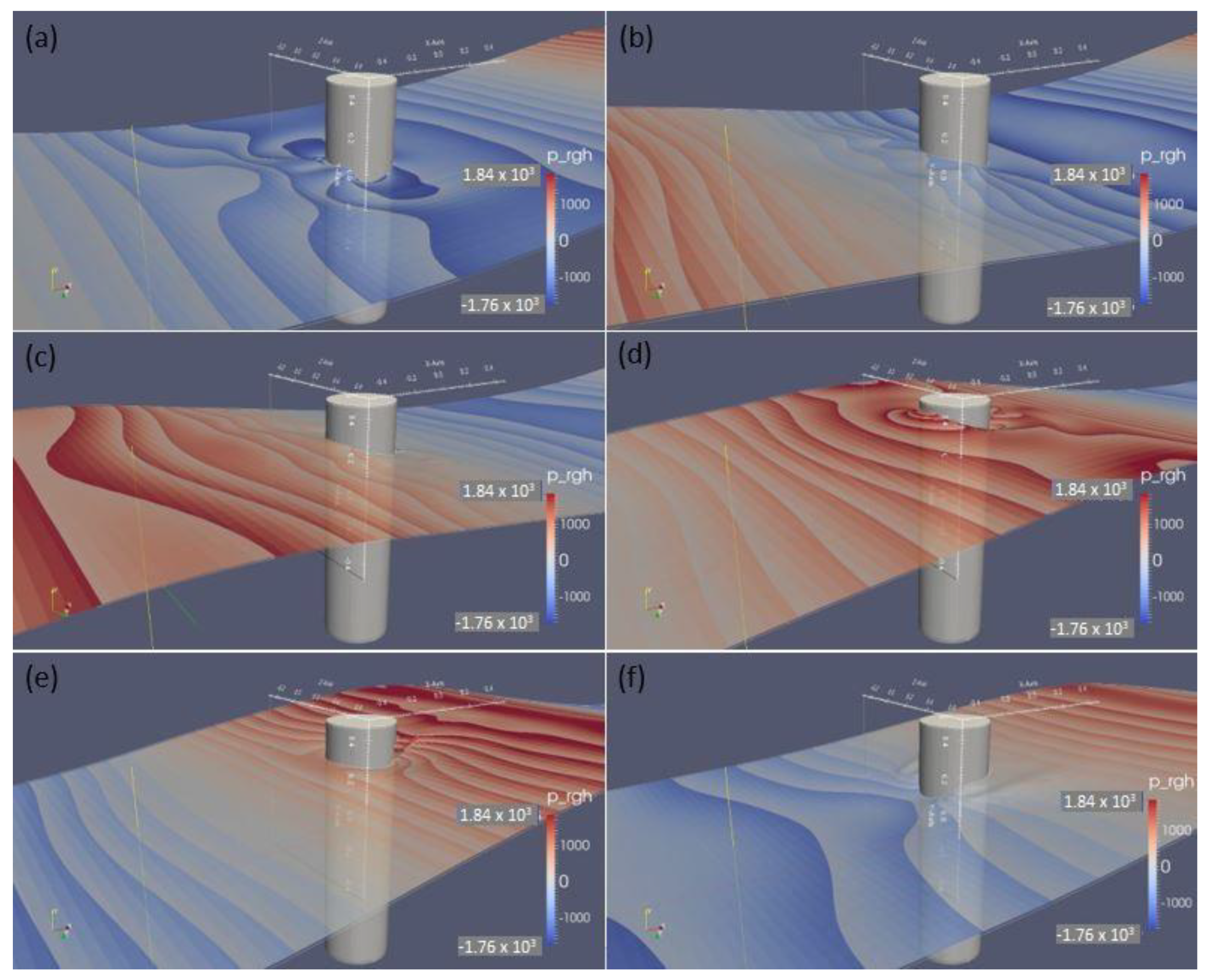
To further illustrate the CFD results, the pressure distribution in the simulation domain is shown in Figure 11 and Figure 12. The figures show the change of pressure in the domain due to the interaction between the cylinder and the incoming waves. They also show the disturbance in the incoming incident waves due to interaction with the diffracted waves by the cylinder.

Figure 11 shows the interaction of the wave crest with the vertical cylinder. The cylinder encounters high horizontal pressure during the interaction, as can be seen from the deep red color near the free surface. The horizontal pressure gradually fades away with increasing water depth. The contours on the cylinder also show the vertical (upward) force encountered by the cylinder during the wave interaction.

Figure 12 shows both the pressure distribution on the free surface during the wave encounter by the cylinder and also reference axis for observing the free-surface elevation. The figure shows how the free surface deforms around the cylinder during wave propagation. The cylinder faces low pressure at the wave trough and the free surface is close to −0.23. Next, the wave passes and when the cylinder encounters the wave peak, there is a jump of the free surface at the front of the cylinder and the wave reaches a height of roughly 0.3. During the wave encounter, the elevation of the free surface at the side and behind the cylinder is lower than that at the front.

4.2. Comparison of Analytical Boussinesq Model (BM) Results against CFD Simulations

A MATLAB code is developed to compute the Bessel and Hankel functions in the analytical solutions using built-in sub-routine Matlab to present numerical results of Boussinesq solutions for locations A, B, C, D, and E (as discussed in Section 3 and labeled in Figure 3).

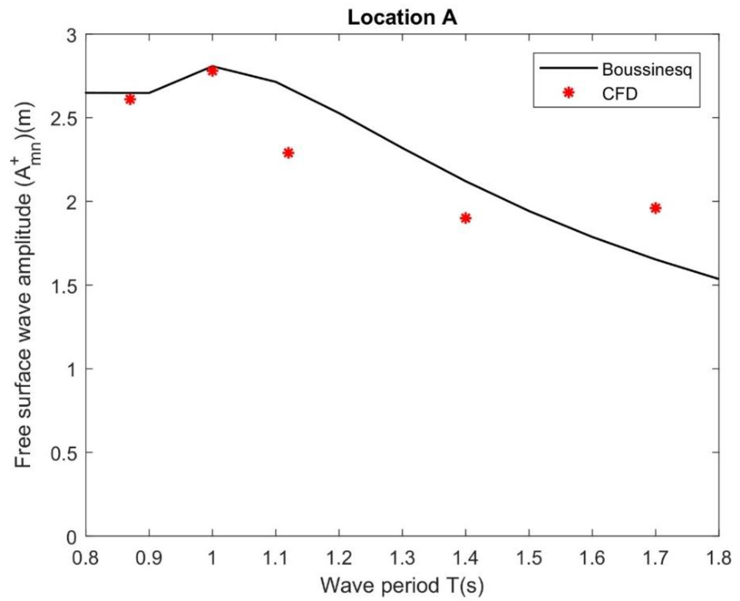
Figure 13, Figure 14, Figure 15, Figure 16 and Figure 17 show the comparisons of results of Boussinesq second-order super-harmonic wave amplitude $A_{mn}^{+}$ against CFD model simulations in the exterior region for locations A, B, D, C, and E, respectively, versus time period T(s). From Figure 13 and Figure 14, it is observed that the peak amplitude of the Boussinesq result agreed well and the wave amplitude trend is similar with CFD model results. However, the wave amplitude in location A is higher than that of location B.

In Figure 15, the results of second-order super-harmonic wave amplitude $A_{mn}^{+}$ are in good agreement between the Boussinesq and CFD model simulations for a smaller wave period in location C (behind the cylinder). However, for higher wave period the results between the two models did not agree well although the trend is similar. This may be due to the numerical errors arising from time and spatial discretization that are more evident with the disagreement of the wave amplitudes in between two models. Furthermore, unlike the CFD simulations, the BM is based on the frequency domain and the numerical model requires some time for the forcing wave to be applied and to stabilize behind the cylinder (location C). This may be the reason to lead the discrepancy in comparison of the Boussinesq results and those of CFD simulations.

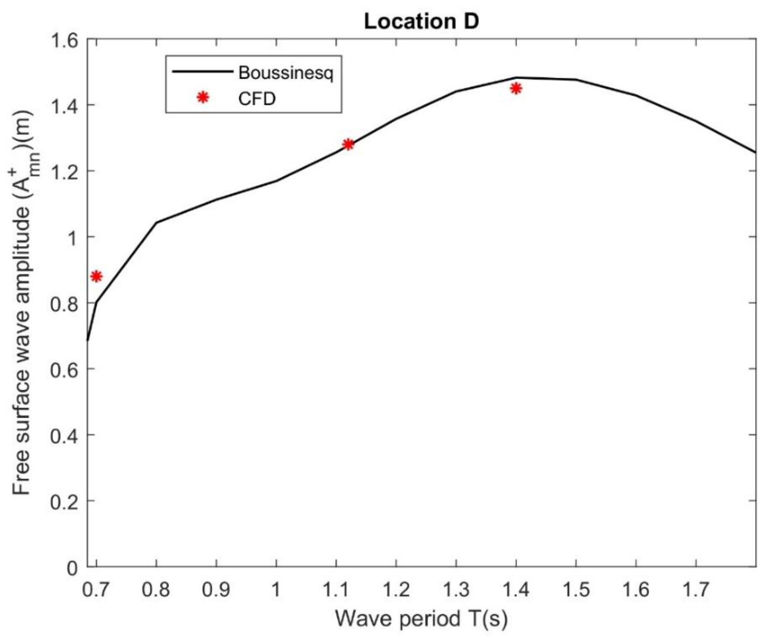
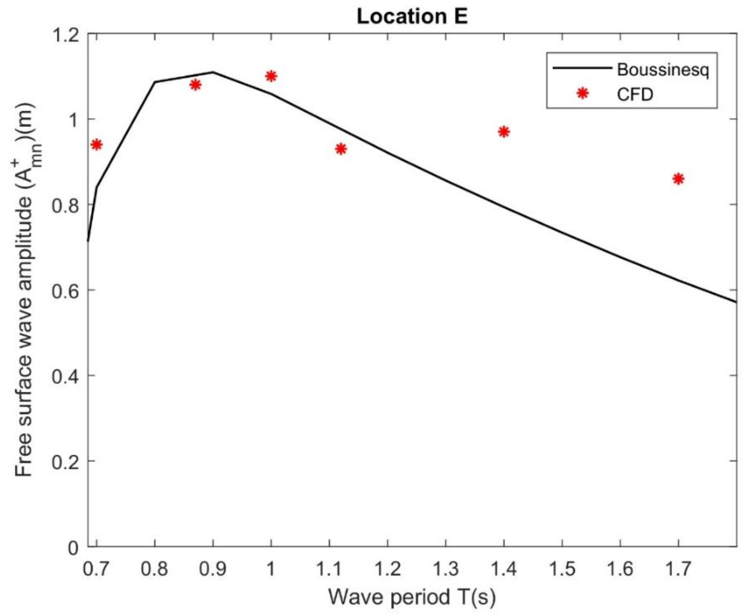
Figure 16 compares the results of second-order super-harmonic wave amplitude $A_{mn}^{+}$ between Boussinesq and CFD model for location D. It is observed that the peak amplitude and trend between the Boussinesq and CFD models are fully agreed. It suggests that the interaction of second-order wave amplitude and vertical cylinder exhibits similar behavior in their trends for both models. In Figure 17, it is found that the observations are similar to those of Figure 13 and Figure 14. However, for the higher wave period, the CFD data points are a little far and they only agree in the trend, not their values. The reason is similar to those of Figure 15.

The next subsection analyses the effect of second-order sub-harmonic waves on the different parameters associated with wave diffraction by a floating fixed truncated vertical cylinder.

4.3. Effect of Design Parameters on Second-Order Sub-Harmonic Wave Amplitudes

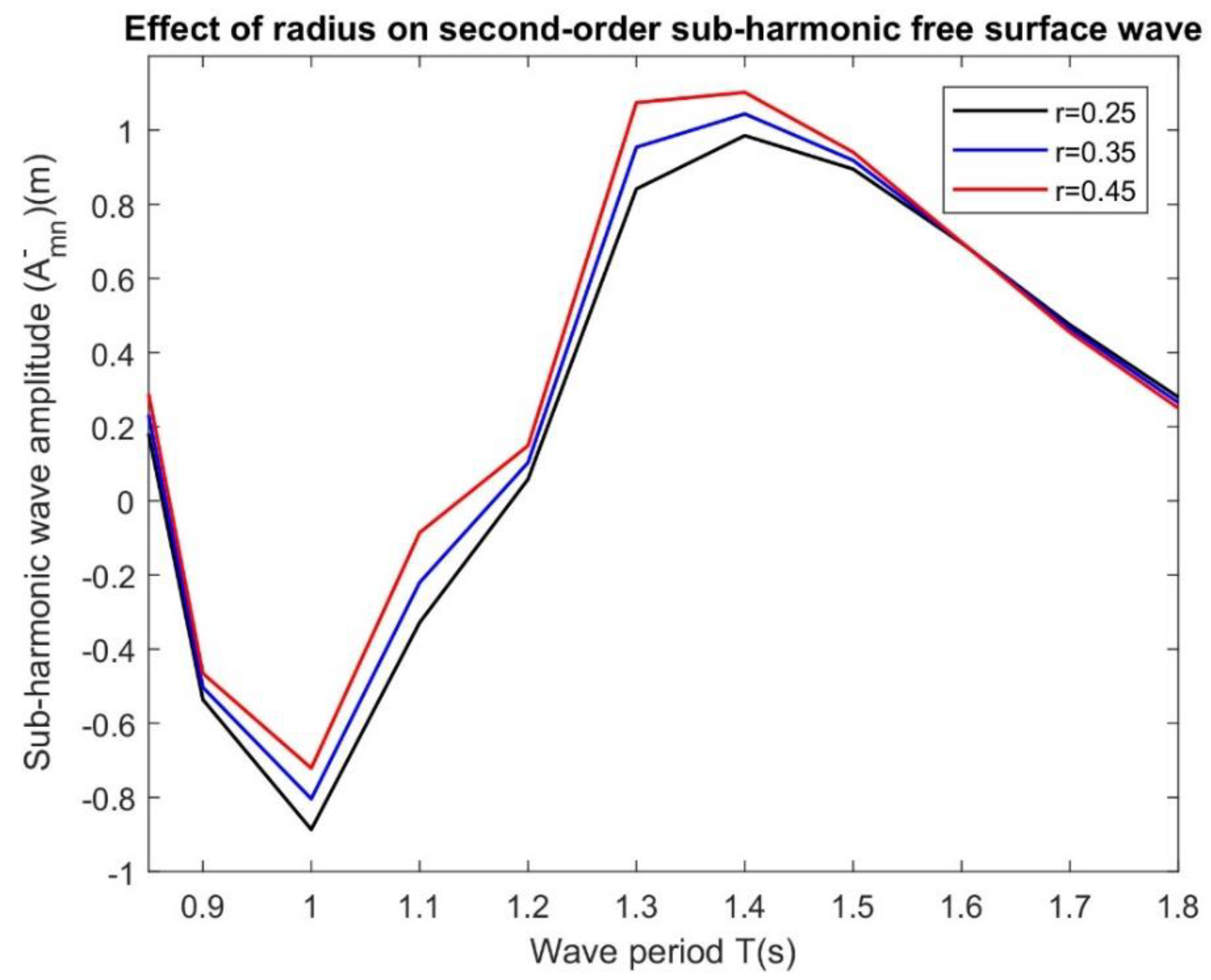
In Figure 18, the effects of radius r on second-order sub-harmonic wave amplitude. $A_{mn}^{-}$ at location B for h = 4.0 m, k_m = 0.84 and z_α = 0.5 versus wave period T(s) is plotted. It is observed that the second-order sub-harmonic wave amplitude $A_{mn}^{-}$ increases with an increase in the radius of the cylinder. The observations are similar to [31] in the case of wave diffraction by a cylinder in two-layer fluids. This may be due to fact that as the cylinder occupied more water plane area, the large amount of incident wave energy concentrates around the structure and on the other hand, physically, this result may be from an increase in fluid momentum as the flow negotiates the cylinder.

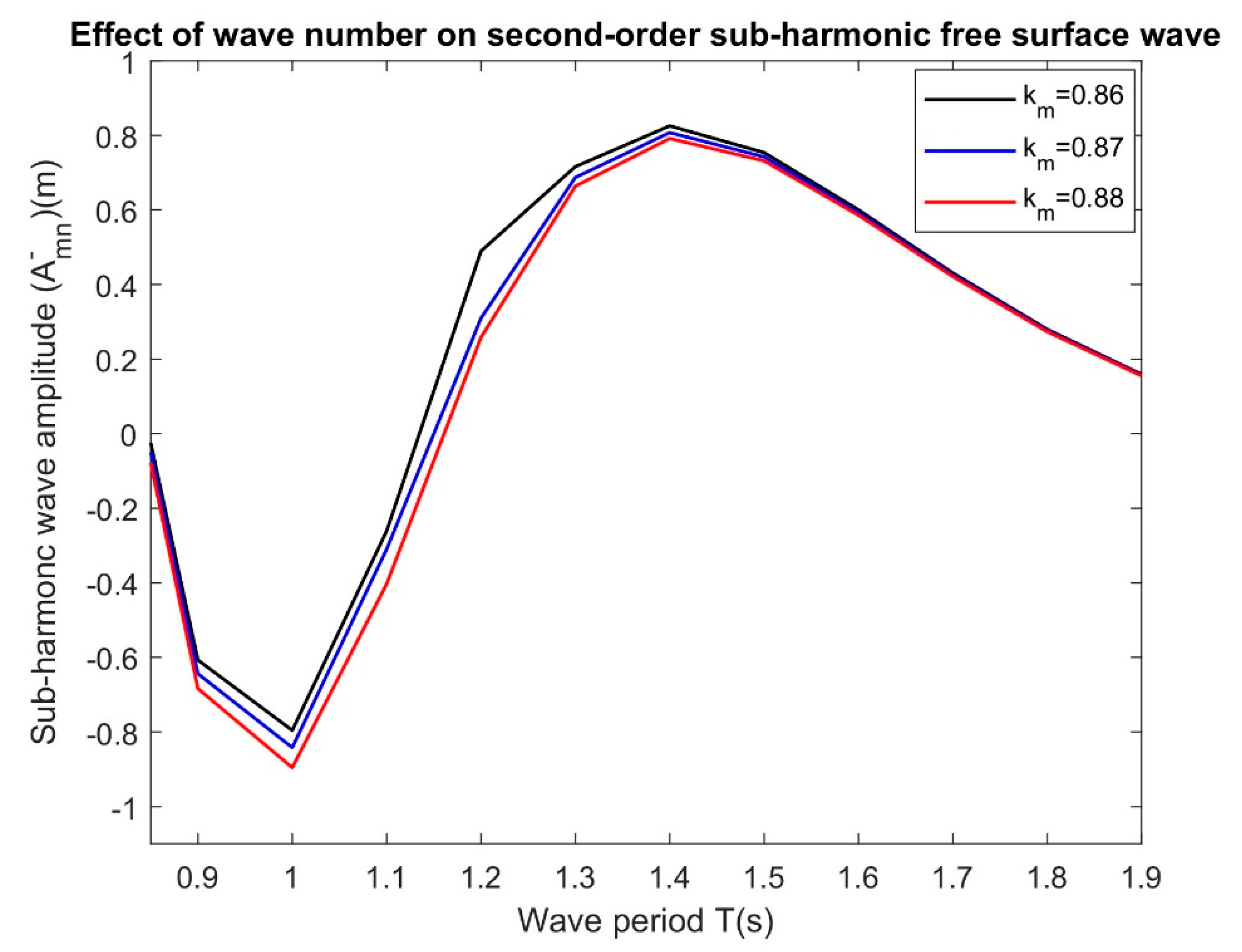
Figure 19 shows the effects of wavenumber k_m on second-order sub-harmonic wave amplitude $A_{mn}^{-}$ at location B for h = 4.0 m, r = 0.35 m and z_α = 0.5 versus wave period T(s). It is observed that the second-order sub-harmonic wave amplitude $A_{mn}^{-}$ decreases with increase in wave number values. Moreover, the observation is similar to [8]. Furthermore, it is seen that for higher wave period the variations of second-order sub-harmonic wave amplitude becomes negligible for fixed values of radius and for different wave number.

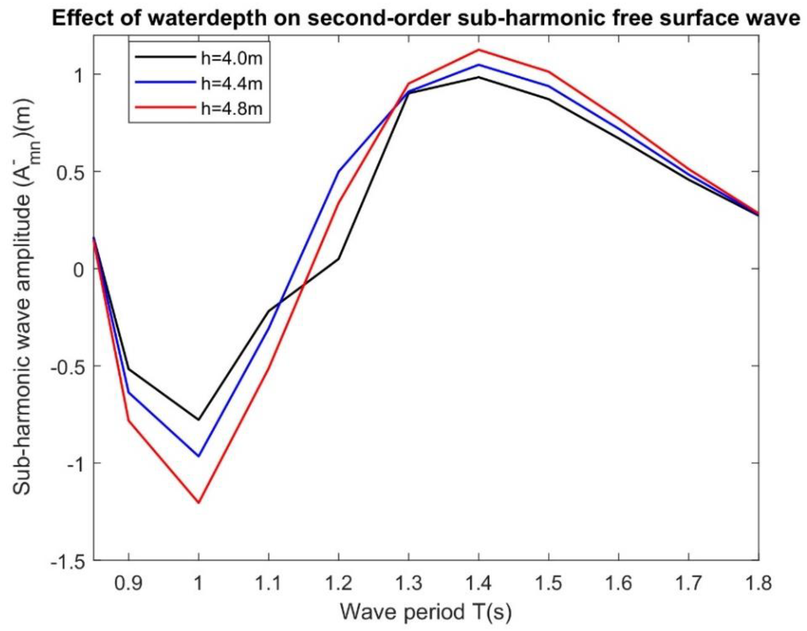
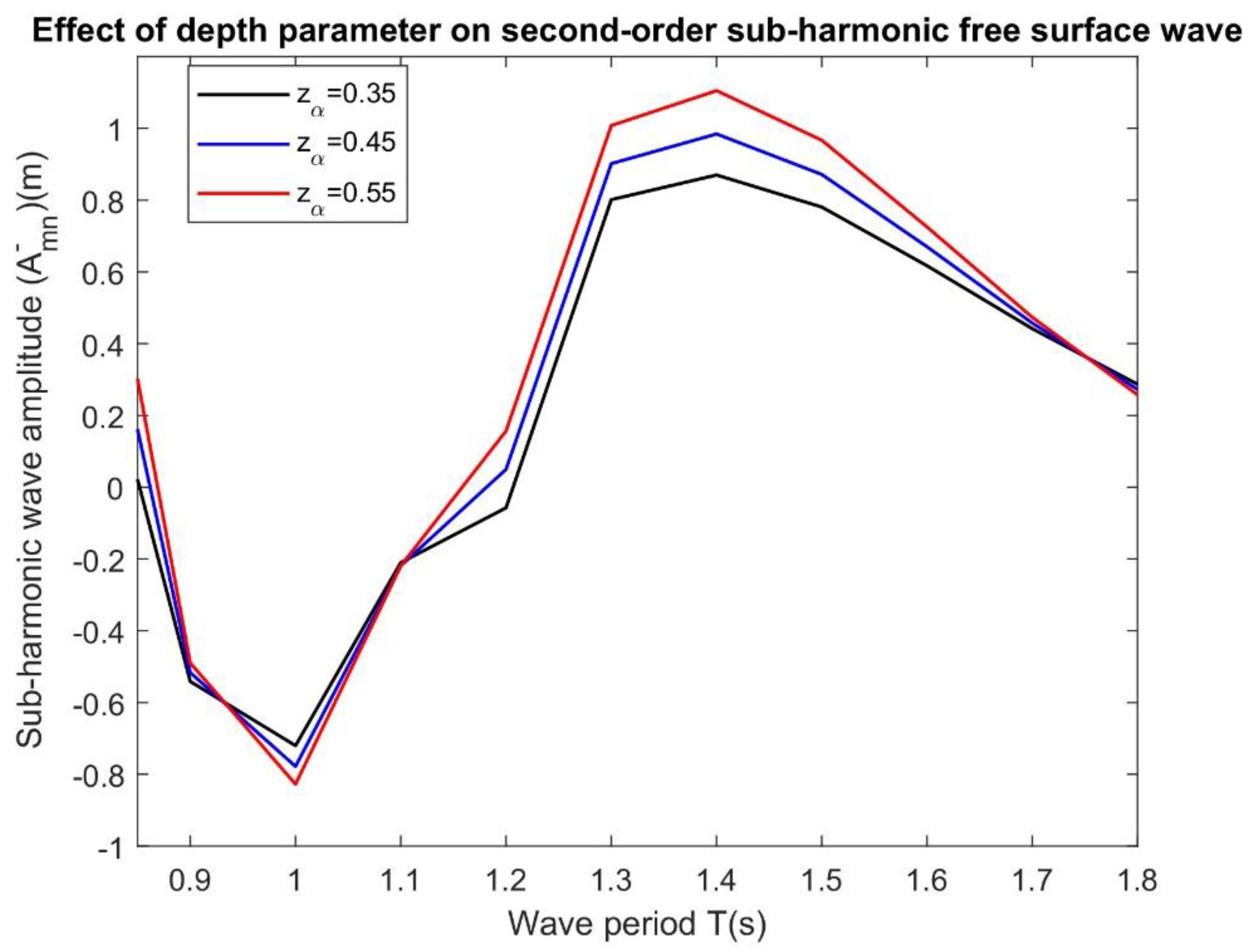
Figure 20 depicts the effects of water depth on second-order sub-harmonic wave amplitude $A_{mn}^{-}$ at location B with r = 0.35 m, k_m = 0.84 and z_α = 0.5 versus wave period T(s). Overall, it is observed that the sub-harmonic second-order wave amplitude decreases with the increase in water depths for higher values of the wave period. This is due to an increase in hydrostatic pressure, the force per unit is exerted by water on the floating cylinder. In Figure 21, the effects of depth parameters on second-order sub-harmonic wave amplitude $A_{mn}^{-}$ at location B for r = 0.35 m, k_m = 0.84 and h = 4.0 m, and versus wave period T(s) is plotted. It is observed that the second-order sub-harmonic wave amplitude $A_{mn}^{-}$ increases with increase in depth parameters whilst the effect is negligible for a smaller wave period.

All numerical computations associated with analytical expressions were performed in a desktop machine with Intel ^® core i7-4790 CPU with 3.60GHz processor and 32 GB of ram memory. On an average, each case took roughly 10–15 min to finish.

5. Discussion

In the theoretical perspective, the contribution of the present boundary value problem is the formulation associated with wave diffraction by a floating fixed truncated vertical cylinder based on Boussinesq-type equations using Bessel’s and Hankel’s functions, which lead to further formulation of the second-order free surface elevation displacement and velocity potentials in the exterior domain. Therefore, importantly, the comparisons of super-harmonic wave amplitude for different probe locations between BM, numerical CFD simulations, experimental, and other numerical data, and some other effects are also discussed in the succeeding paragraphs.

Initially, in order to show efficiency and level of exactness of the CFD model simulations relative to other methods, the results of wave amplitudes and wave heights from CFD are compared against EFD and numerical data available in the literature for the different probe locations. It is found that the CFD results here show reasonable agreement with experimental data; although the values do not exactly agree, the trend is well captured. For almost all cases, CFD under predicts the results compared to EFD results. The slight deviation might be explained to some extent by the location of the probe in CFD model. In CFD, the probe was set 5 mm away from the cylinder, whereas, in experiments, it was exactly on the cylinder. This could not be done in the CFD model since probes in simulation can only capture data from a cell, not at voids. The numerical dissipation of incoming waves and instability of the turbulence model at the free surface also contributes to the under prediction. In general, the CFD results agree better with the NS model results, compared to the immersed boundary method results, since the present CFD model also follows the RANS model. Overall, the CFD results show reasonable agreement with the experimental and other numerical data, as presented in Figure 5, Figure 6, Figure 7, Figure 8 and Figure 9.

Then, the numerical results of second-order super-harmonic wave amplitudes obtained from BM are compared with CFD results in the same probe locations. It is observed that the peak amplitudes are in good agreement between the two models and the trend of the wave profiles are similar in nature for all cases, as shown in Figure 13, Figure 14, Figure 15, Figure 16 and Figure 17. However, the CFD data points are little far from the BM results. These differences can be justified by the full non-linearity solution and viscous effects of the CFD model, while the solution of the analytical model is only of second-order. However, the comparison showed that the developed BM is supported by the numerical CFD model which indicates that the BM may be reliable for concept validation and further enhancement of the model to study motion characteristics of the cylinder to design a floating point absorber wave energy converter.

Regarding the force and pressure distribution analysis, it may be mentioned that the value of the horizontal force is in between the vertical force and moment acting on the vertical cylinder. The peak amplitude of moment is higher than those of horizontal and vertical force. Regarding the pressure distribution around the cylinder, it is found that during the wave encounter, the free surface elevation at the side and behind the cylinder is lower than that at the front probe location.

Finally, the effects of radius, wave number, water depth, and depth parameters on the second-order sub-harmonic wave amplitudes from the Boussinesq results are analyzed, as presented in Figure 18, Figure 19, Figure 20 and Figure 21. It is observed that the second-order subharmonic waves around the cylinder are negative for all cases whilst, in the same range the super-harmonic waves are positive as presented in Figure 13, Figure 14, Figure 15, Figure 16 and Figure 17. Furthermore, it is seen that the effects of the second-order on super-harmonic waves for free surface wave profiles around the cylinder are stronger than those of sub-harmonics as in [8].

6. Conclusions

The difference between the paper [2] and the present one is the presence of detailed Boussinesq formulation and the analytical expressions for the second-order super- and sub-harmonic wave amplitudes of the BM and more wave period cases in CFD simulation under the consideration of turbulent flow. Furthermore, one more comparison result for the wave gauge behind the cylinder between Boussinesq and CFD simulations is studied, the CFD results for wave forces, moment, and pressure distribution around the cylinder are presented and discussed, and finally, a new section is added to investigate the effect of second-order sub-harmonic waves on the cylinder for different design parameters from BM.

The innovation of this study is the development of BM based on BEs and numerical CFD simulations associated with the vertical truncated cylinder and providing benchmark results by comparing various methodologies of non-linear/second-order super- and sub-harmonic incoming wave amplitudes/wave heights interactions, as these phenomena have central importance during the design of WECs. On the other hand, the horizontal and vertical forces and pitch moment acting on the vertical truncated cylinder are newly added to this study. It has been observed that:

• The CFD results generated using OpenFOAM for wave heights/wave elevations showed reasonable agreement with experimental and other numerical models for all the cases. CFD simulations also predicted results for horizontal and vertical forces and moments encountered by the cylinder.
• The results of second-order super-harmonic wave amplitude were compared with CFD results and it was found that they are in good agreement and the trends are also well captured in all cases.
• The effects of second-order super-harmonic waves are stronger than those of sub-harmonic waves around the cylinder, and the complicated transformation process in the wave amplitude distribution is found to be due to the phase interaction between the flows around and below the cylinder.
• The CFD pressure distribution indicates that the wave elevation at the side and behind of the cylinder is lower than that at the front. From the computational point of view, the present study indicates that the CFD is far more expensive compared to BM and perhaps is best suited for final design validation for WEC devices, rather than the design iteration stage.
• As a result, the present BM can be used with confidence to generalize for heaving motion characteristics of the floating vertical truncated cylinder to design point absorber floating WEC.
• Furthermore, the wave force results of the CFD modeling may help to use in the future BM model to analyze the level of fidelity by comparing them.

References

- Lannes, D. On the Dynamics of Floating Structures. Ann. PDE 2017, 3, 11. [Google Scholar] [CrossRef] [Green Version]
- Mohapatra, S.C.; Islam, H.; Guedes Soares, C. Wave diffraction by a floating fixed truncated vertical cylinder based on Boussinesq equations. In Advances in Renewable Energies; Guedes Soares, C., Ed.; Taylor & Francis: London, UK, 2019; pp. 281–289. [Google Scholar]
- Yu, S.M.P. A theoretical investigation on the wave forces on the multiple cylinders in shallow water. Appl. Math. Mech. 1987, 8, 377–387. [Google Scholar]
- Basmat, A.; Ziegler, F. Interaction of a Plane Solitary Wave with a Rigid Vertical Cylinder. ZAMM 1998, 78, 535–543. [Google Scholar] [CrossRef]
- Kang, A.; Lin, P.; Lee, Y.J.; Zhu, B. Numerical simulation of wave interaction with vertical circular cylinders of different submergences using immersed boundary method. Comput. Fluids 2015, 106, 41–53. [Google Scholar] [CrossRef]
- Mohapatra, S.C.; Guedes Soares, C. Wave forces on a floating structure over flat bottom based on Boussinesq formulation. In Renewable Energies Offshore; Guedes Soares, C., Ed.; Taylor & Francis Group: London, UK, 2015; pp. 335–342. [Google Scholar]
- Gadelho, J.F.M.; Mohapatra, S.C.; Guedes Soares, C. CFD analysis of a fixed floating box-type structure under regular waves. In Developments in Maritime Transportation and Harvesting of Sea Resources; Guedes Soares, C., Teixeira, A.P., Eds.; Taylor & Francis Group: London, UK, 2018; pp. 513–520. [Google Scholar]
- Mohapatra, S.C.; Gadelho, J.F.M.; Guedes Soares, C. Effect of interfacial tension on internal waves based on Boussinesq equations in two-layer fluids. J. Coast. Res. 2018, 35, 445–462. [Google Scholar] [CrossRef]
- Liu, Z.B.; Fang, K.Z.; Cheng, Y.Z. A new multi-layer irrotational Boussinesq-type model for highly nonlinear and dispersive surface waves over a mild slope seabed. J. Fluid Mech. 2018, 842, 323–353. [Google Scholar] [CrossRef]
- Parvizi, M.; Khodadadian, A.; Eslahchi, M.R. Analysis of Ciarlet–Raviart mixed finite element methods for solving damped Boussinesq equation. J. Comput. Appl. Math. 2020, 379, 112818. [Google Scholar] [CrossRef]
- Abbaszadeh, M.; Dehghan, M.; Khodadadian, A.; Heitzinger, C. Analysis and application of the interpolating element free Galerkin (IEFG) method to simulate the prevention of groundwater contamination with application in fluid flow. J. Comput. Appl. Math. 2020, 368, 112453. [Google Scholar] [CrossRef]
- Mohammadi, V.; Dehghan, M.; Khodadadian, A.; Wick, T. Numerical investigation on the transport equation in spherical coordinates via generalized moving least squares and moving kriging least-squares approximations. Eng. Comput. 2019. [Google Scholar] [CrossRef]
- Eskilsson, C.; Palm, J.; Ensig-Karup, A.; Bosi, U.; Ricchiuto, M. Wave induced motions of point-absorbers: An hierarchical investigation of hydrodynamic models. In Proceedings of the European Wave And Tidal Energy Conference (EWTEC 2015), Nantes, France, 6–11 September 2015. [Google Scholar]
- Palm, J.; Eskilsson, C.; Paredes, G.M.; Bergdahl, L. Coupled mooring analysis for floating wave energy converters using CFD: Formulation and validation. Int. J. Mar. Energy 2016, 16, 83–99. [Google Scholar] [CrossRef] [Green Version]
- Lavrov, A.; Guedes Soares, C. Modelling the Heave Oscillations of Vertical Cylinders with Damping Plates. Int. J. Marit. Eng. 2016, 158, A187–A197. [Google Scholar]
- Bihs, H.; Kamata, A.; Lu, Z.J.; Arntsen, I.A. Simulation of floating bodies using a combined immersed boundary with the level set method in REEF3D. In Proceedings of the VII International Conference on Computational Methods in Marine Engineering, Nantes, France, 15–17 June 2017. [Google Scholar]
- Elhanafi, A.; Duffy, J.; Macfarlane, G.; Binns, J.; Keough, S.J. Experimental validation of a CFD model for inline force and bow wave height on a vertical cylinder moving in waves. In Proceedings of the Thirteenth Pacific-Asia Offshore Mechanics Symposium, Jeju, Korea, 14–17 October 2018. [Google Scholar]
- Yu, Y.; Li, Y. Reynolds-averaged Navier–Stokes simulation of the heave performance of a two-body floating-point absorber wave energy system. Comput. Fluids 2013, 73, 104–114. [Google Scholar] [CrossRef]
- Yu, Y.; Li, Y. Preliminary results of a RANS simulation for a floating-point absorber wave energy system under extreme wave conditions. In Proceedings of the 30th International Conference on Ocean, Offshore and Arctic Engineering (OMAE 2011), Rotterdam, The Netherlands, 19–24 June 2011. [Google Scholar]
- Trulsen, K.; Teigen, P. Wave scattering around a vertical cylinder: Fully nonlinear potential flow calculations compared with low order perturbation results and experiments. In Proceedings of the 21th International Conference on Offshore Mechanics and Arctic Engineering, Oslo, Norway, 23–28 June 2002. [Google Scholar]
- Cong, D.; Shang, J.; Luo, Z.; Sun, C.; Wu, W. Energy Efficiency Analysis of Multi-Type Floating Bodies for a Novel Heaving Point Absorber with Application to Low-Power Unmanned Ocean Device. Energies 2018, 11, 3282. [Google Scholar] [CrossRef] [Green Version]
- Mohseni, M.; Esperanca, P.T.; Sphaier, S.H. Numerical study of wave run-up on a fixed and vertical surface-piercing cylinder subjected to regular, non-breaking waves using OpenFOAM. Ocean Eng. 2018, 79, 228–252. [Google Scholar] [CrossRef]
- Islam, H.; Mohapatra, S.C.; Guedes Soares, C. Comparisons of CFD, experimental, and analytical simulations of a heaving box-type floating structure. In Progress in Maritime Technology and Engineering; Guedes Soares, C., Santos, T.A., Eds.; Taylor & Francis Group: London, UK, 2018; pp. 513–520. [Google Scholar]
- Mohapatra, S.C.; Fonseca, R.B.; Guedes Soares, C. Comparison of Analytical and Numerical Simulations of Long Nonlinear Internal Waves in Shallow Water. J. Coast. Res. 2017, 34, 928–938. [Google Scholar] [CrossRef]
- Mohapatra, S.C.; Guedes Soares, C. Comparing solutions of the coupled Boussinesq equations in shallow water. In Maritime Technology and Engineering; Guedes Soares, C., Santos, T.A., Eds.; Taylor & Francis Group: London, UK, 2015; pp. 947–954. [Google Scholar]
- Mohapatra, S.C.; Fonseca, R.B.; Guedes Soares, C. A comparison between analytical and numerical simulations of solutions of the coupled Boussinesq equations. In Maritime Technology and Engineering 3; Guedes Soares, C., Santos, T.A., Eds.; Taylor & Francis Group: London, UK, 2016; pp. 1175–1180. [Google Scholar]
- Nwogu, O.; Takayama, T.; Ikeda, N. Numerical Simulation of the Shoaling of Irregular Waves Using a New Boussinesq Model. In Report of the Port and Harbour Research Institute; PARI: Nagase, Yokosuka, Japan, 1992; Volume 31, pp. 3–19. [Google Scholar]
- Jasak, H. OpenFOAM: Open Source CFD in research and industry. Int. J. Nav. Arch. Ocean Eng. 2009, 1, 89–94. [Google Scholar]
- Mercier, R.S.; Niedzwecki, J.M. Experimental measurements of second order diffraction by a truncated vertical cylinder in monochromatic waves. In Proceedings of the 7th International Conference on the Behaviour of Offshore Structures, Cambridge, MA, USA, 12–15 July 1994; Volume 2, pp. 265–287. [Google Scholar]
- Park, J.C.; Kim, M.H.; Miyata, H. Fully non-linear free-surface simulations by a 3D viscous numerical wave tank. Int. J. Num. Methods Fluids 1999, 29, 685–703. [Google Scholar] [CrossRef]
- Harun, F.N. Analytical solution for wave diffraction around cylinder. Res. J. Recent Sci. 2013, 2, 5–10. [Google Scholar]
Figure 1.
Schematic diagram of wave diffraction by a floating fixed truncated vertical cylinder.
Figure 2.
Overall simulation domain for the vertical truncated cylinder (a), mesh distribution on the side (b) and top (c) of the domain.
Figure 3.
Schematic diagram of the simulation case setup, (a) top view and (b) side view of the setup.
Figure 4.
General assembly of the simulation domain.
Figure 5.
Comparison between computational fluid dynamics (CFD), experimental and numerical data of wave amplitude and heights for location A [5,25,26].
Figure 6.
Comparison between CFD, experimental and numerical data of wave amplitude and heights for location B [5,25,26].
Figure 7.
Comparison between CFD, experimental and numerical data of wave amplitude and heights for location C [5,25,26].
Figure 8.
Comparison between CFD, experimental and numerical data of wave amplitude and heights for location D [5,25,26].
Figure 9.
Comparison between CFD, experimental and numerical data of wave amplitude and heights for location E [5,25,26].
Figure 10.
Non-dimensional horizontal force Fx, vertical force Fy, and pitch moment Mz acting on the truncated cylinder at different wave periods.
Figure 11.
Pressure distribution in the simulation domain from the side, while the cylinder interacts with the incoming wave crest with simulation time for figure (a) 0.19Ts, (b) 0.0.25Ts, (c) 0.31Ts and (d) 0.37Ts. The flow field pressure distribution is for case 9, with wave period of T = 2.50 s and wave height of H = 0.46 m.
Figure 12.
Pressure distribution in the simulation domain from the top, while the cylinder interacts with the incoming wave with simulation time for figure (a) 0.28Ts, (b) 0.43Ts, (c) 0.57Ts, (d) 0.71Ts, (e) 86Ts and (f) 1Ts. The flow field pressure distribution is for case 9, with wave period of T = 2.50 s and wave height of H = 0.46 m.
Figure 13.
Comparison of Boussinesq, second-order super-harmonic wave amplitude in Equation (29) and CFD models of free surface elevation for location A.
Figure 14.
Comparison of Boussinesq, second-order super-harmonic wave amplitude in Equation (29) and CFD models of free surface elevation for location B.
Figure 15.
Comparison of Boussinesq, second-order super-harmonic wave amplitude in Equation (29) and CFD models of free surface elevation for location C.
Figure 16.
Comparison of Boussinesq, second-order super-harmonic wave amplitude in Equation (29) and CFD models of free surface elevation for location D.
Figure 17.
Comparison of Boussinesq, second-order super-harmonic wave amplitude in Equation (29) and CFD models of free surface elevation for location E.
Figure 18.
Effects of radius of the cylinder r on second-order sub-harmonic wave amplitude of Equation (29) in location B for h = 4.0 m, km = 0.84 and zα = 0.5.
Figure 19.
Effects of wavenumber km on second-order sub-harmonic wave amplitude of Equation (29) at location B with h = 4.0 m, r = 0.35 m and zα = 0.5.
Figure 20.
Effects of water depth on second-order sub-harmonic wave amplitude of Equation (29) at the location B with r = 0.35 m, km = 0.84 and zα = 0.5.
Figure 21.
Effects of depth parameter at a specific elevation zα on second-order sub-harmonic wave amplitudes of Equation (29) at location B for r = 0.35 m, km = 0.84 and h = 4.0 m.