Daily Water Level Prediction of Zrebar Lake (Iran): A Comparison between M5P, Random Forest, Random Tree and Reduced Error Pruning Trees Algorithms

 ,
,  , ,
, ,  ,
,
Abstract
:1. Introduction
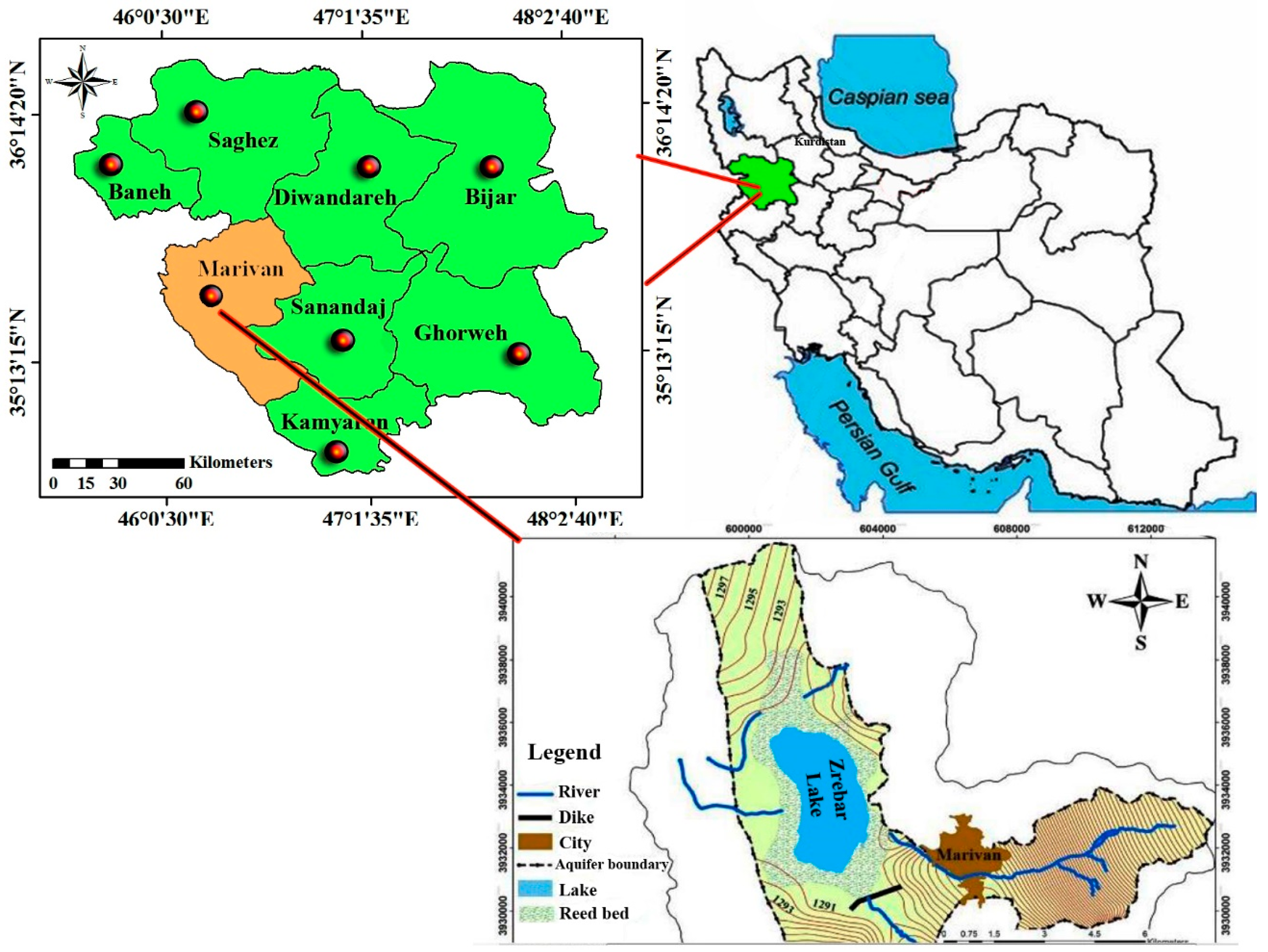
2. Study Area
3. Materials and Methods
3.1. Data Assemblage and Preparation
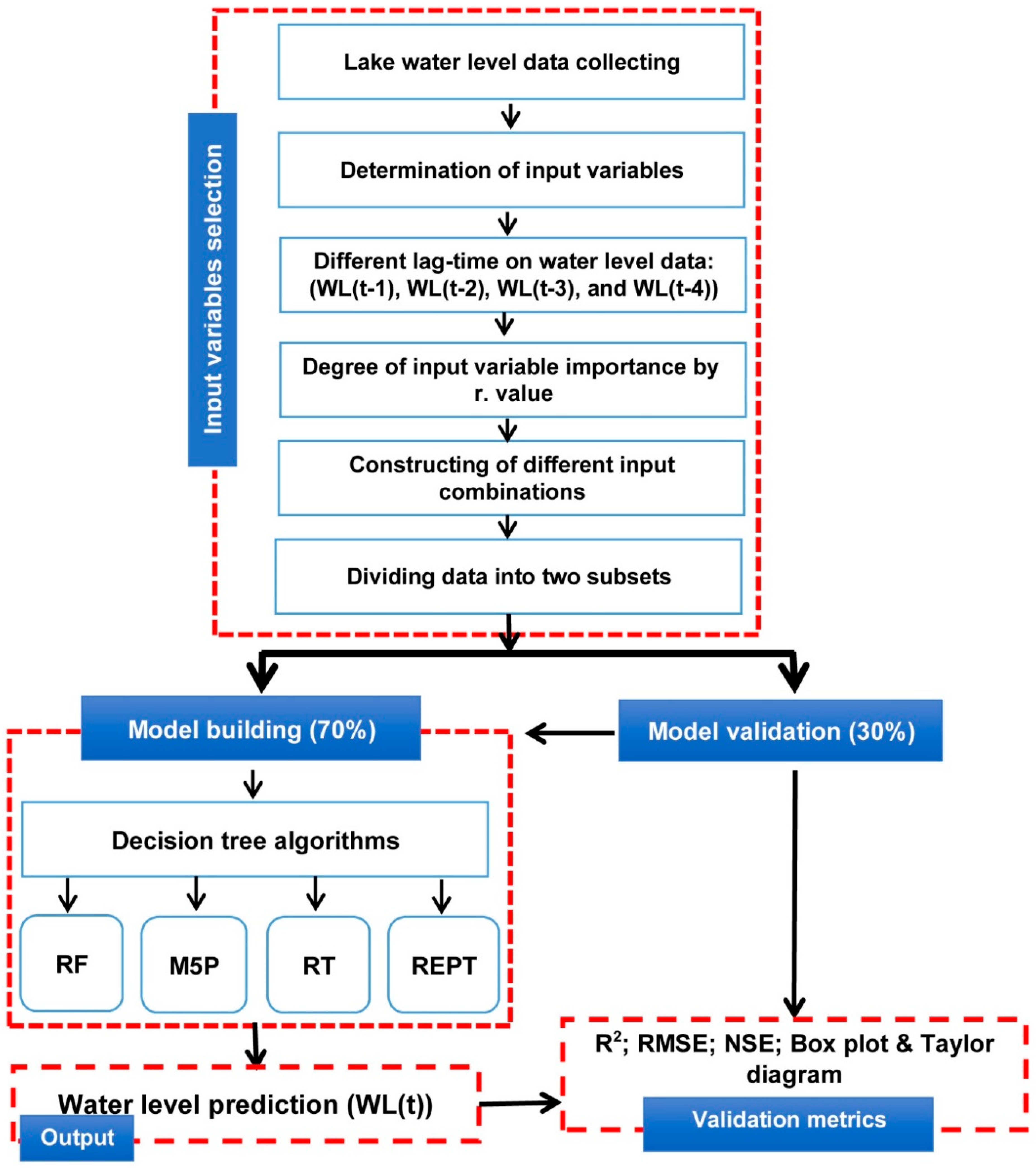
3.2. Methodology
3.2.1. M5P
3.2.2. Random Forest (RF)
3.2.3. Random Tree (RT)
3.2.4. Reduced Error Pruning Tree (REPT)
3.2.5. Model Evaluation and Comparison
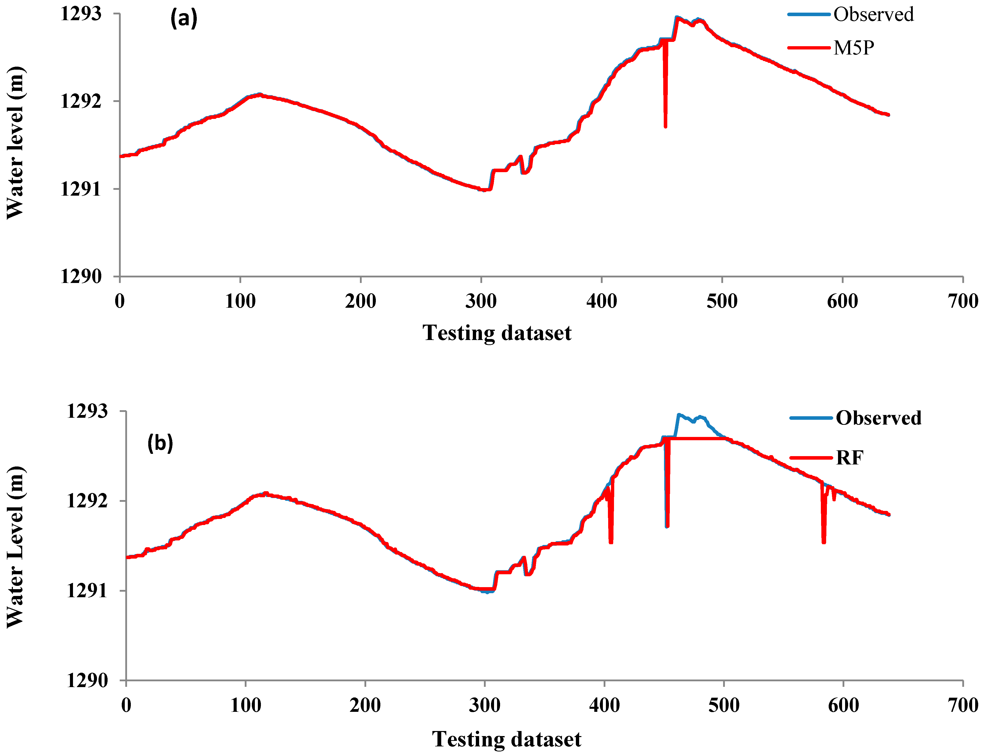
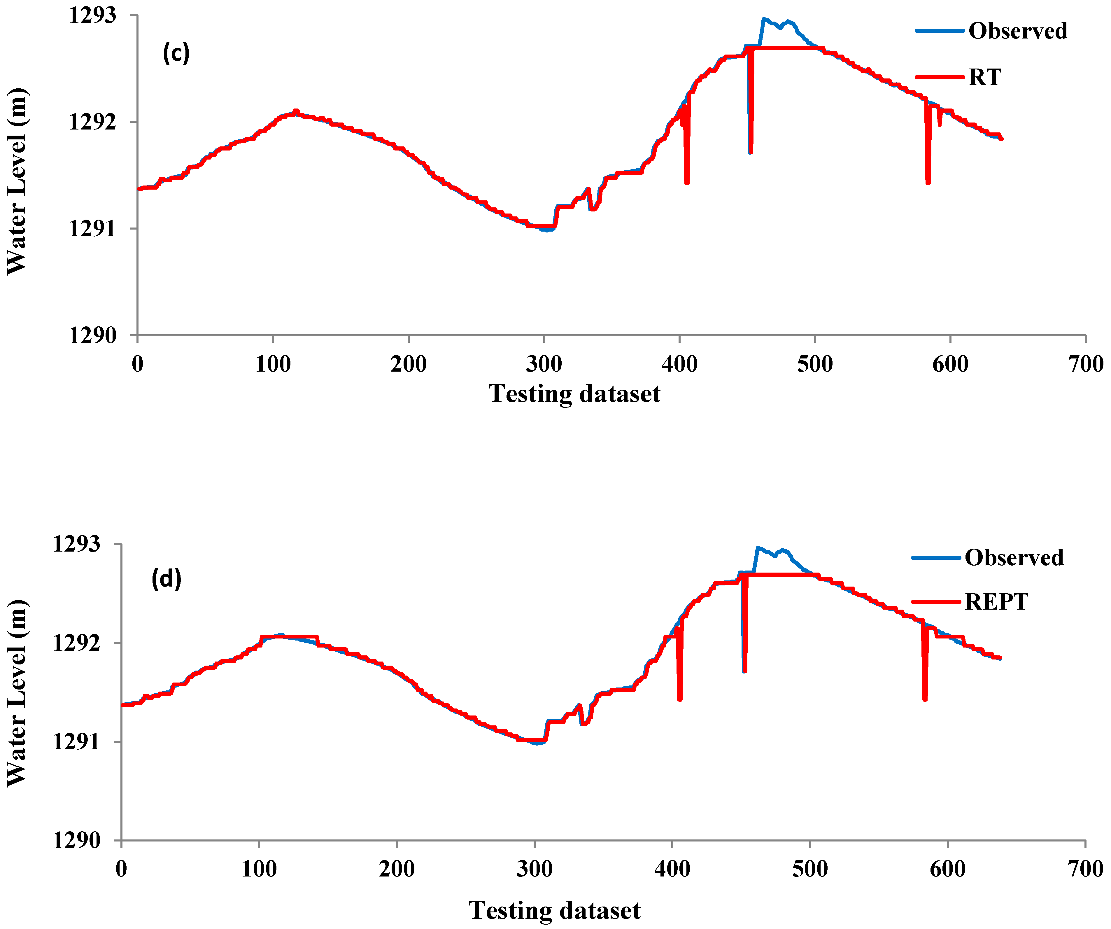
4. Results and Analysis
5. Discussion
6. Conclusions
Author Contributions
Funding
Conflicts of Interest
References
- Vuglinskiy, V. Water Level in Lakes and Reservoirs, Water Storage; Global Terrestrial Observing System: Rome, Italy, 2009. Available online: http://www.fao.org/gtos/doc/ECVs/T04/T04.pdf (accessed on 21 July 2020).
- Hwang, C.; Cheng, Y.-S.; Han, J.; Kao, R.; Huang, C.-Y.; Wei, S.-H.; Wang, H. Multi-decadal monitoring of lake level changes in the qinghai-tibet plateau by the topex/poseidon-family altimeters: Climate implication. Remote Sens. 2016, 8, 446. [Google Scholar] [CrossRef] [Green Version]
- Karimi, S.; Shiri, J.; Kisi, O.; Makarynskyy, O. Forecasting water level fluctuations of urmieh lake using gene expression programming and adaptive neuro-fuzzy inference system. Int. J. Ocean Clim. Syst. 2012, 3, 109–125. [Google Scholar] [CrossRef] [Green Version]
- Altunkaynak, A. Forecasting surface water level fluctuations of lake van by artificial neural networks. Water Resour. Manag. 2007, 21, 399–408. [Google Scholar] [CrossRef]
- Kisi, O.; Shiri, J.; Nikoofar, B. Forecasting daily lake levels using artificial intelligence approaches. Comput. Geosci. 2012, 41, 169–180. [Google Scholar] [CrossRef]
- Rahmati, O.; Choubin, B.; Fathabadi, A.; Coulon, F.; Soltani, E.; Shahabi, H.; Mollaefar, E.; Tiefenbacher, J.; Cipullo, S.; Ahmad, B.B. Predicting uncertainty of machine learning models for modelling nitrate pollution of groundwater using quantile regression and uneec methods. Sci. Total Environ. 2019, 688, 855–866. [Google Scholar] [CrossRef]
- Tien Bui, D.; Shirzadi, A.; Chapi, K.; Shahabi, H.; Pradhan, B.; Pham, B.T.; Singh, V.P.; Chen, W.; Khosravi, K.; Bin Ahmad, B. A hybrid computational intelligence approach to groundwater spring potential mapping. Water 2019, 11, 2013. [Google Scholar] [CrossRef] [Green Version]
- Chen, W.; Pradhan, B.; Li, S.; Shahabi, H.; Rizeei, H.M.; Hou, E.; Wang, S. Novel hybrid integration approach of bagging-based fisher’s linear discriminant function for groundwater potential analysis. Nat. Resour. Res. 2019, 28, 1239–1258. [Google Scholar] [CrossRef] [Green Version]
- Rahmati, O.; Naghibi, S.A.; Shahabi, H.; Bui, D.T.; Pradhan, B.; Azareh, A.; Rafiei-Sardooi, E.; Samani, A.N.; Melesse, A.M. Groundwater spring potential modelling: Comprising the capability and robustness of three different modeling approaches. J. Hydrol. 2018, 565, 248–261. [Google Scholar] [CrossRef]
- Leira, M.; Cantonati, M. Effects of Water-Level Fluctuations on Lakes: An Annotated Bibliography. In Ecological Effects of Water-Level Fluctuations in Lakes; Springer: Berlin/Heidelberg, Germany, 2008; pp. 171–184. [Google Scholar]
- Dai, X.; Wan, R.; Yang, G. Non-stationary water-level fluctuation in china’s poyang lake and its interactions with yangtze river. J. Geogr. Sci. 2015, 25, 274–288. [Google Scholar] [CrossRef] [Green Version]
- Ahmadlou, M.; Karimi, M.; Alizadeh, S.; Shirzadi, A.; Parvinnejhad, D.; Shahabi, H.; Panahi, M. Flood susceptibility assessment using integration of adaptive network-based fuzzy inference system (anfis) and biogeography-based optimization (bbo) and bat algorithms (ba). Geocarto Int. 2019, 34, 1252–1272. [Google Scholar] [CrossRef]
- Naghibi, S.A.; Pourghasemi, H.R. A comparative assessment between three machine learning models and their performance comparison by bivariate and multivariate statistical methods in groundwater potential mapping. Water Resour. Manag. 2015, 29, 5217–5236. [Google Scholar] [CrossRef]
- Bowden, G.J.; Maier, H.R.; Dandy, G.C. Optimal division of data for neural network models in water resources applications. Water Resour. Res. 2002, 38, 2-1-2-11. [Google Scholar] [CrossRef] [Green Version]
- Pradhan, B. Flood susceptible mapping and risk area delineation using logistic regression, gis and remote sensing. J. Spat. Hydrol. 2010, 9, 1–18. [Google Scholar]
- Kia, M.B.; Pirasteh, S.; Pradhan, B.; Mahmud, A.R.; Sulaiman, W.N.A.; Moradi, A. An artificial neural network model for flood simulation using gis: Johor river basin, malaysia. Environ. Earth Sci. 2012, 67, 251–264. [Google Scholar] [CrossRef]
- Tehrany, M.S.; Pradhan, B.; Jebur, M.N. Flood susceptibility mapping using a novel ensemble weights-of-evidence and support vector machine models in gis. J. Hydrol. 2014, 512, 332–343. [Google Scholar] [CrossRef]
- Choubin, B.; Moradi, E.; Golshan, M.; Adamowski, J.; Sajedi-Hosseini, F.; Mosavi, A. An ensemble prediction of flood susceptibility using multivariate discriminant analysis, classification and regression trees, and support vector machines. Sci. Total Environ. 2019, 651, 2087–2096. [Google Scholar] [CrossRef]
- Abbaszadeh, P.; Alipour, A.; Asadi, S. Development of a coupled wavelet transform and evolutionary l evenberg-m arquardt neural networks for hydrological process modeling. Comput. Intell. 2018, 34, 175–199. [Google Scholar] [CrossRef]
- Asadi, S. Evolutionary fuzzification of ripper for regression: Case study of stock prediction. Neurocomputing 2019, 331, 121–137. [Google Scholar] [CrossRef]
- Asadi, S.; Shahrabi, J. Complexity-based parallel rule induction for multiclass classification. Inf. Sci. 2017, 380, 53–73. [Google Scholar] [CrossRef]
- Chen, W.; Li, Y.; Xue, W.; Shahabi, H.; Li, S.; Hong, H.; Wang, X.; Bian, H.; Zhang, S.; Pradhan, B. Modeling flood susceptibility using data-driven approaches of naïve bayes tree, alternating decision tree, and random forest methods. Sci. Total Environ. 2020, 701, 134979. [Google Scholar] [CrossRef] [PubMed]
- Shahabi, H.; Shirzadi, A.; Ghaderi, K.; Omidvar, E.; Al-Ansari, N.; Clague, J.J.; Geertsema, M.; Khosravi, K.; Amini, A.; Bahrami, S. Flood detection and susceptibility mapping using sentinel-1 remote sensing data and a machine learning approach: Hybrid intelligence of bagging ensemble based on k-nearest neighbor classifier. Remote Sens. 2020, 12, 266. [Google Scholar] [CrossRef] [Green Version]
- Wang, Y.; Hong, H.; Chen, W.; Li, S.; Panahi, M.; Khosravi, K.; Shirzadi, A.; Shahabi, H.; Panahi, S.; Costache, R. Flood susceptibility mapping in dingnan county (china) using adaptive neuro-fuzzy inference system with biogeography based optimization and imperialistic competitive algorithm. J. Environ. Manag. 2019, 247, 712–729. [Google Scholar] [CrossRef]
- Chen, W.; Hong, H.; Li, S.; Shahabi, H.; Wang, Y.; Wang, X.; Ahmad, B.B. Flood susceptibility modelling using novel hybrid approach of reduced-error pruning trees with bagging and random subspace ensembles. J. Hydrol. 2019, 575, 864–873. [Google Scholar] [CrossRef]
- Khosravi, K.; Melsse, A.M.; Shahabi, H.; Shirzadi, A.; Chapi, K.; Hong, H. Flood Susceptibility Mapping at Ningdu Catchment, China Using Bivariate and Data Mining Techniques. In Extreme Hydrology and Climate Variability; Elsevier: Amsterdam, The Netherlands, 2019; pp. 419–434. [Google Scholar]
- Tien Bui, D.; Khosravi, K.; Shahabi, H.; Daggupati, P.; Adamowski, J.F.; Melesse, A.M.; Thai Pham, B.; Pourghasemi, H.R.; Mahmoudi, M.; Bahrami, S. Flood spatial modeling in northern iran using remote sensing and gis: A comparison between evidential belief functions and its ensemble with a multivariate logistic regression model. Remote Sens. 2019, 11, 1589. [Google Scholar] [CrossRef] [Green Version]
- Bui, D.T.; Panahi, M.; Shahabi, H.; Singh, V.P.; Shirzadi, A.; Chapi, K.; Khosravi, K.; Chen, W.; Panahi, S.; Li, S. Novel hybrid evolutionary algorithms for spatial prediction of floods. Sci. Rep. 2018, 8, 1–14. [Google Scholar] [CrossRef] [PubMed] [Green Version]
- Tien Bui, D.; Khosravi, K.; Li, S.; Shahabi, H.; Panahi, M.; Singh, V.P.; Chapi, K.; Shirzadi, A.; Panahi, S.; Chen, W. New hybrids of anfis with several optimization algorithms for flood susceptibility modeling. Water 2018, 10, 1210. [Google Scholar] [CrossRef] [Green Version]
- Shafizadeh-Moghadam, H.; Valavi, R.; Shahabi, H.; Chapi, K.; Shirzadi, A. Novel forecasting approaches using combination of machine learning and statistical models for flood susceptibility mapping. J. Environ. Manag. 2018, 217, 1–11. [Google Scholar] [CrossRef] [Green Version]
- Khosravi, K.; Pham, B.T.; Chapi, K.; Shirzadi, A.; Shahabi, H.; Revhaug, I.; Prakash, I.; Bui, D.T. A comparative assessment of decision trees algorithms for flash flood susceptibility modeling at haraz watershed, northern iran. Sci. Total Environ. 2018, 627, 744–755. [Google Scholar] [CrossRef]
- Nourani, V.; Komasi, M.; Mano, A. A multivariate ann-wavelet approach for rainfall–runoff modeling. Water Resour. Manag. 2009, 23, 2877. [Google Scholar] [CrossRef]
- Wu, C.; Chau, K. Rainfall–runoff modeling using artificial neural network coupled with singular spectrum analysis. J. Hydrol. 2011, 399, 394–409. [Google Scholar] [CrossRef] [Green Version]
- Bae, D.-H.; Jeong, D.M.; Kim, G. Monthly dam inflow forecasts using weather forecasting information and neuro-fuzzy technique. Hydrol. Sci. J. 2007, 52, 99–113. [Google Scholar] [CrossRef] [Green Version]
- Bai, Y.; Chen, Z.; Xie, J.; Li, C. Daily reservoir inflow forecasting using multiscale deep feature learning with hybrid models. J. Hydrol. 2016, 532, 193–206. [Google Scholar] [CrossRef]
- Noori, R.; Karbassi, A.; Moghaddamnia, A.; Han, D.; Zokaei-Ashtiani, M.; Farokhnia, A.; Gousheh, M.G. Assessment of input variables determination on the svm model performance using pca, gamma test, and forward selection techniques for monthly stream flow prediction. J. Hydrol. 2011, 401, 177–189. [Google Scholar] [CrossRef]
- Yaseen, Z.M.; El-Shafie, A.; Jaafar, O.; Afan, H.A.; Sayl, K.N. Artificial intelligence based models for stream-flow forecasting: 2000–2015. J. Hydrol. 2015, 530, 829–844. [Google Scholar] [CrossRef]
- Cigizoglu, H.K.; Kisi, Ö. Methods to improve the neural network performance in suspended sediment estimation. J. Hydrol. 2006, 317, 221–238. [Google Scholar] [CrossRef]
- Kisi, O.; Shiri, J. River suspended sediment estimation by climatic variables implication: Comparative study among soft computing techniques. Comput. Geosci. 2012, 43, 73–82. [Google Scholar] [CrossRef]
- Eslamian, S.; Abedi-Koupai, J.; Amiri, M.; Gohari, S. Estimation of daily reference evapotranspiration using support vector. Res. J. Environ. Sci. 2009, 3, 439–447. [Google Scholar]
- Mehdizadeh, S. Estimation of daily reference evapotranspiration (eto) using artificial intelligence methods: Offering a new approach for lagged eto data-based modeling. J. Hydrol. 2018, 559, 794–812. [Google Scholar] [CrossRef]
- Khosravi, K.; Shahabi, H.; Pham, B.T.; Adamowski, J.; Shirzadi, A.; Pradhan, B.; Dou, J.; Ly, H.-B.; Gróf, G.; Ho, H.L. A comparative assessment of flood susceptibility modeling using multi-criteria decision-making analysis and machine learning methods. J. Hydrol. 2019, 573, 311–323. [Google Scholar] [CrossRef]
- Hong, H.; Tsangaratos, P.; Ilia, I.; Liu, J.; Zhu, A.-X.; Chen, W. Application of fuzzy weight of evidence and data mining techniques in construction of flood susceptibility map of poyang county, china. Sci. Total Environ. 2018, 625, 575–588. [Google Scholar] [CrossRef] [PubMed]
- Tahan, M.H.; Asadi, S. Emdid: Evolutionary multi-objective discretization for imbalanced datasets. Inf. Sci. 2018, 432, 442–461. [Google Scholar] [CrossRef]
- Tahan, M.H.; Asadi, S. Memod: A novel multivariate evolutionary multi-objective discretization. Soft Comput. 2018, 22, 301–323. [Google Scholar] [CrossRef]
- Khosravi, K.; Cooper, J.R.; Daggupati, P.; Pham, B.T.; Bui, D.T. Bedload transport rate prediction: Application of novel hybrid data mining techniques. J. Hydrol. 2020, 124774. [Google Scholar] [CrossRef]
- Khosravi, K.; Barzegar, R.; Miraki, S.; Adamowski, J.; Daggupati, P.; Alizadeh, M.R.; Pham, B.T.; Alami, M.T. Stochastic modeling of groundwater fluoride contamination: Introducing lazy learners. Groundwater 2019. [Google Scholar] [CrossRef]
- Bui, D.T.; Khosravi, K.; Tiefenbacher, J.; Nguyen, H.; Kazakis, N. Improving prediction of water quality indices using novel hybrid machine-learning algorithms. Sci. Total Environ. 2020, 721, 137612. [Google Scholar] [CrossRef]
- Bui, D.T.; Khosravi, K.; Karimi, M.; Busico, G.; Khozani, Z.S.; Nguyen, H.; Mastrocicco, M.; Tedesco, D.; Cuoco, E.; Kazakis, N. Enhancing nitrate and strontium concentration prediction in groundwater by using new data mining algorithm. Sci. Total Environ. 2020, 715, 136836. [Google Scholar] [CrossRef]
- Salih, S.Q.; Sharafati, A.; Khosravi, K.; Faris, H.; Kisi, O.; Tao, H.; Ali, M.; Yaseen, Z.M. River suspended sediment load prediction based on river discharge information: Application of newly developed data mining models. Hydrol. Sci. J. 2019, 65, 624–637. [Google Scholar] [CrossRef]
- Imani, S.; Niksokhan, M.H.; Jamshidi, S.; Abbaspour, K.C. Discharge permit market and farm management nexus: An approach for eutrophication control in small basins with low-income farmers. Environ. Monit. Assess. 2017, 189, 346. [Google Scholar] [CrossRef]
- Imani, S.; Delavar, M.; Niksokhan, M.H. Identification of nutrients critical source areas with swat model under limited data condition. Water Resour. 2019, 46, 128–137. [Google Scholar] [CrossRef]
- Gavili, S.; Javadi, S.; Banihabib, M.; Sanikhani, H. Comparison of intelligent models to predict water level fluctuations in zarivar lake considering groundwater level. Iran-Water Resour. Res. 2018, 14, 339–344. [Google Scholar]
- Bahrami, S.; Wigand, E. Daily streamflow forecasting using nonlinear echo state network. Int. J. Adv. Res. Sci. Eng. Technol. 2018, 5, 3619–3625. [Google Scholar]
- Hu, C.; Wan, F. Input Selection in Learning Systems: A Brief Review of Some Important Issues and Recent Developments. In Proceedings of the 2009 IEEE International Conference on Fuzzy Systems, Jeju Island, Korea, 20–24 August 2009; pp. 530–535. [Google Scholar]
- Sharafati, A.; Khosravi, K.; Khosravinia, P.; Ahmed, K.; Salman, S.A.; Yaseen, Z.M.; Shahid, S. The potential of novel data mining models for global solar radiation prediction. Int. J. Environ. Sci. Technol. 2019, 16, 7147–7164. [Google Scholar] [CrossRef]
- Ayele, G.T.; Teshale, E.Z.; Yu, B.; Rutherfurd, I.D.; Jeong, J. Streamflow and sediment yield prediction for watershed prioritization in the upper blue nile river basin, ethiopia. Water 2017, 9, 782. [Google Scholar] [CrossRef] [Green Version]
- Taheri, K.; Shahabi, H.; Chapi, K.; Shirzadi, A.; Gutiérrez, F.; Khosravi, K. Sinkhole susceptibility mapping: A comparison between bayes-based machine learning algorithms. Land Degrad. Dev. 2019, 30, 730–745. [Google Scholar] [CrossRef]
- Pham, B.T.; Prakash, I.; Khosravi, K.; Chapi, K.; Trinh, P.T.; Ngo, T.Q.; Hosseini, S.V.; Bui, D.T. A comparison of support vector machines and bayesian algorithms for landslide susceptibility modelling. Geocarto Int. 2019, 34, 1385–1407. [Google Scholar] [CrossRef]
- Chen, W.; Hong, H.; Panahi, M.; Shahabi, H.; Wang, Y.; Shirzadi, A.; Pirasteh, S.; Alesheikh, A.A.; Khosravi, K.; Panahi, S. Spatial prediction of landslide susceptibility using gis-based data mining techniques of anfis with whale optimization algorithm (woa) and grey wolf optimizer (gwo). Appl. Sci. 2019, 9, 3755. [Google Scholar] [CrossRef] [Green Version]
- Khosravi, K.; Daggupati, P.; Alami, M.T.; Awadh, S.M.; Ghareb, M.I.; Panahi, M.; Pham, B.T.; Rezaie, F.; Qi, C.; Yaseen, Z.M. Meteorological data mining and hybrid data-intelligence models for reference evaporation simulation: A case study in iraq. Comput. Electron. Agric. 2019, 167, 105041. [Google Scholar] [CrossRef]
- Khozani, Z.S.; Khosravi, K.; Pham, B.T.; Kløve, B.; Mohtar, W.; Melini, W.H.; Yaseen, Z.M. Determination of compound channel apparent shear stress: Application of novel data mining models. J. Hydroinform. 2019, 21, 798–811. [Google Scholar] [CrossRef] [Green Version]
- Quinlan, J.R. Combining Instance-Based and Model-Based Learning. In Proceedings of the Tenth International Conference on Machine Learning, Amherst, MA, USA, 27–29 June 1993; pp. 236–243. [Google Scholar]
- Khosravi, K.; Mao, L.; Kisi, O.; Yaseen, Z.M.; Shahid, S. Quantifying hourly suspended sediment load using data mining models: Case study of a glacierized andean catchment in chile. J. Hydrol. 2018, 567, 165–179. [Google Scholar] [CrossRef]
- Breiman, L. Random forests. Mach. Learn. 2001, 45, 5–32. [Google Scholar] [CrossRef] [Green Version]
- Breiman, L. Bagging predictors. Mach. Learn. 1996, 24, 123–140. [Google Scholar] [CrossRef] [Green Version]
- Aldous, D.; Pitman, J. Inhomogeneous continuum random trees and the entrance boundary of the additive coalescent. Probab. Theory Relat. Fields 2000, 118, 455–482. [Google Scholar] [CrossRef] [Green Version]
- LaValle, S.M. Rapidly-Exploring Random Trees: A New Tool for Path Planning; Citeseer: University Park, PA, USA, 1998. [Google Scholar]
- Polo, J.M.; Liu, S.; Figueroa, M.E.; Kulalert, W.; Eminli, S.; Tan, K.Y.; Apostolou, E.; Stadtfeld, M.; Li, Y.; Shioda, T. Cell type of origin influences the molecular and functional properties of mouse induced pluripotent stem cells. Nat. Biotechnol. 2010, 28, 848–855. [Google Scholar] [CrossRef] [PubMed] [Green Version]
- Mohamed, W.N.H.W.; Salleh, M.N.M.; Omar, A.H. A Comparative Study of Reduced Error Pruning Method in Decision Tree Algorithms. In Proceedings of the 2012 IEEE International Conference on Control System, Computing and Engineering, Penang, Malaysia, 23–25 November 2012; pp. 392–397. [Google Scholar]
- Taylor, K.E. Summarizing multiple aspects of model performance in a single diagram. J. Geophys. Res. Atmos. 2001, 106, 7183–7192. [Google Scholar] [CrossRef]
- Houghton, J.T. The Scientific Basis; Contribution of Working Group I to the Third Assessment Report of the Intergovernmental Panel on Climate Change; Cambridge University Press: Cambridge, MA, USA, 2001. [Google Scholar]
- Santhi, C.; Arnold, J.G.; Williams, J.R.; Dugas, W.A.; Srinivasan, R.; Hauck, L.M. Validation of the swat model on a large rwer basin with point and nonpoint sources 1. JAWRA J. Am. Water Resour. Assoc. 2001, 37, 1169–1188. [Google Scholar] [CrossRef]
- Nash, J.E.; Sutcliffe, J.V. River flow forecasting through conceptual models part I—A discussion of principles. J. Hydrol. 1970, 10, 282–290. [Google Scholar] [CrossRef]
- Moriasi, D.N.; Arnold, J.G.; Van Liew, M.W.; Bingner, R.L.; Harmel, R.D.; Veith, T.L. Model evaluation guidelines for systematic quantification of accuracy in watershed simulations. Trans. ASABE 2007, 50, 885–900. [Google Scholar] [CrossRef]
- Gupta, H.V.; Sorooshian, S.; Yapo, P.O. Status of automatic calibration for hydrologic models: Comparison with multilevel expert calibration. J. Hydrol. Eng. 1999, 4, 135–143. [Google Scholar] [CrossRef]
- Legates, D.R.; McCabe, G.J., Jr. Evaluating the use of “goodness-of-fit” measures in hydrologic and hydroclimatic model validation. Water Resour. Res. 1999, 35, 233–241. [Google Scholar] [CrossRef]
- Behzad, M.; Asghari, K.; Coppola, E.A., Jr. Comparative study of svms and anns in aquifer water level prediction. J. Comput. Civ. Eng. 2010, 24, 408–413. [Google Scholar] [CrossRef]
- Yoon, H.; Jun, S.-C.; Hyun, Y.; Bae, G.-O.; Lee, K.-K. A comparative study of artificial neural networks and support vector machines for predicting groundwater levels in a coastal aquifer. J. Hydrol. 2011, 396, 128–138. [Google Scholar] [CrossRef]
- Kisi, O.; Shiri, J.; Karimi, S.; Shamshirband, S.; Motamedi, S.; Petković, D.; Hashim, R. A survey of water level fluctuation predicting in urmia lake using support vector machine with firefly algorithm. Appl. Math. Comput. 2015, 270, 731–743. [Google Scholar] [CrossRef]
- Shiri, J.; Shamshirband, S.; Kisi, O.; Karimi, S.; Bateni, S.M.; Nezhad, S.H.H.; Hashemi, A. Prediction of water-level in the urmia lake using the extreme learning machine approach. Water Resour. Manag. 2016, 30, 5217–5229. [Google Scholar] [CrossRef]
- Sahoo, S.; Russo, T.A.; Elliott, J.; Foster, I. Machine learning algorithms for modeling groundwater level changes in agricultural regions of the us. Water Resour. Res. 2017, 53, 3878–3895. [Google Scholar] [CrossRef]
- Nhu, V.-H.; Rahmati, O.; Falah, F.; Shojaei, S.; Al-Ansari, N.; Shahabi, H.; Shirzadi, A.; Górski, K.; Nguyen, H.; Ahmad, B.B. Mapping of groundwater spring potential in karst aquifer system using novel ensemble bivariate and multivariate models. Water 2020, 12, 985. [Google Scholar] [CrossRef] [Green Version]
- Chen, W.; Zhao, X.; Tsangaratos, P.; Shahabi, H.; Ilia, I.; Xue, W.; Wang, X.; Ahmad, B.B. Evaluating the usage of tree-based ensemble methods in groundwater spring potential mapping. J. Hydrol. 2020, 583, 124602. [Google Scholar] [CrossRef]
- Chen, W.; Li, Y.; Tsangaratos, P.; Shahabi, H.; Ilia, I.; Xue, W.; Bian, H. Groundwater spring potential mapping using artificial intelligence approach based on kernel logistic regression, random forest, and alternating decision tree models. Appl. Sci. 2020, 10, 425. [Google Scholar] [CrossRef] [Green Version]
- Balouchi, B.; Nikoo, M.R.; Adamowski, J. Development of expert systems for the prediction of scour depth under live-bed conditions at river confluences: Application of different types of anns and the m5p model tree. Appl. Soft Comput. 2015, 34, 51–59. [Google Scholar] [CrossRef]
- Almasi, S.N.; Bagherpour, R.; Mikaeil, R.; Ozcelik, Y.; Kalhori, H. Predicting the building stone cutting rate based on rock properties and device pullback amperage in quarries using m5p model tree. Geotech. Geol. Eng. 2017, 35, 1311–1326. [Google Scholar] [CrossRef]
- Sihag, P.; Karimi, S.M.; Angelaki, A. Random forest, m5p and regression analysis to estimate the field unsaturated hydraulic conductivity. Appl. Water Sci. 2019, 9, 129. [Google Scholar] [CrossRef] [Green Version]
- Yi, H.-S.; Lee, B.; Park, S.; Kwak, K.-C.; An, K.-G. Short-term algal bloom prediction in juksan weir using m5p model-tree and extreme learning machine. Environ. Eng. Res. 2018. [Google Scholar] [CrossRef]
- Onyari, E.K.; Ilunga, F. Application of mlp neural network and m5p model tree in predicting streamflow: A case study of luvuvhu catchment, south africa. Int. J. Innov. Manag. Technol. 2013, 4, 11. [Google Scholar]


| No | Different Input Combinations | Output |
|---|---|---|
| 1 | WL(t-1) | WL(t) |
| 2 | WL(t-1), WL(t-2) | WL(t) |
| 3 | WL(t-1), WL(t-2) WL(t-3) | WL(t) |
| 4 | WL(t-1), WL(t-2), WL(t-3), WL(t-4) | WL(t) |
| 5 | WL(t-1), WL(t-2), WL(t-3), WL(t-4), WL(t-5) | WL(t) |
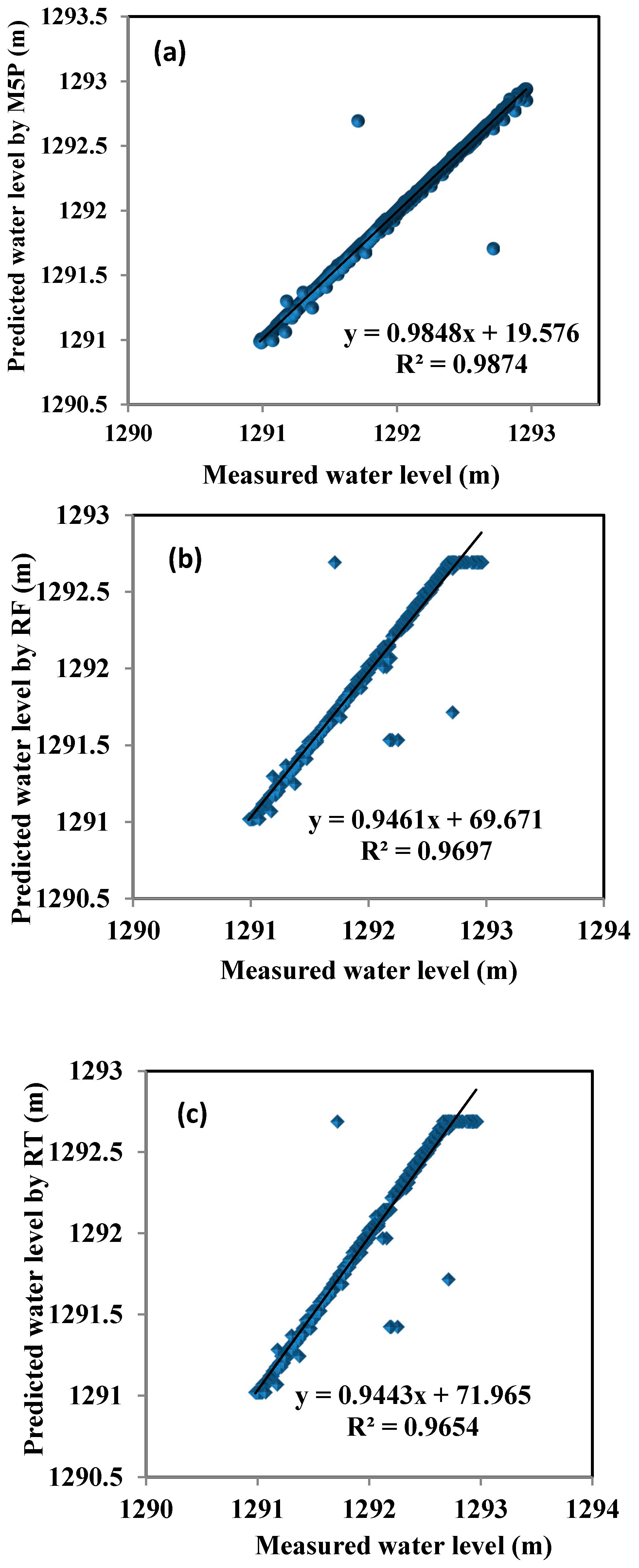
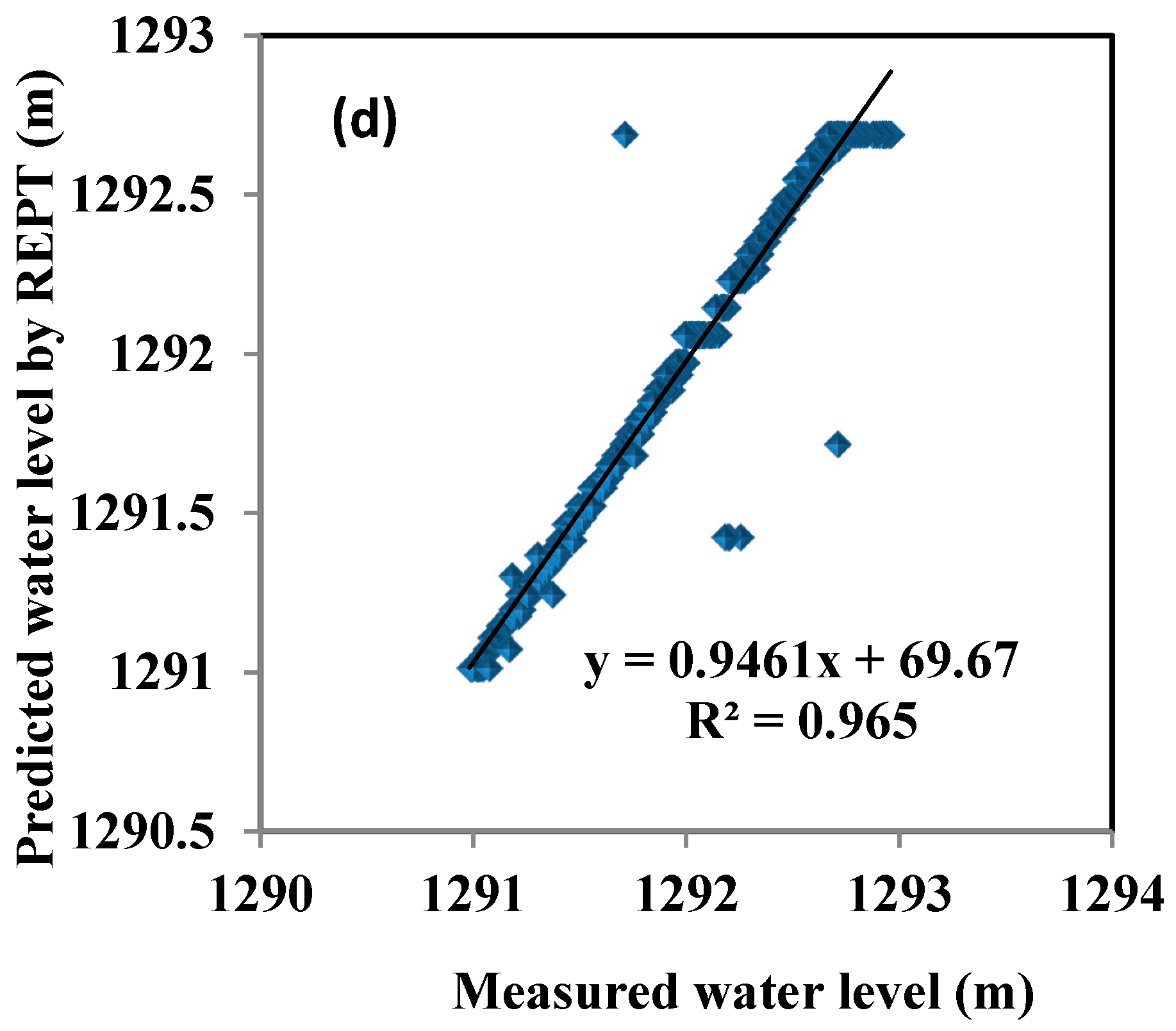
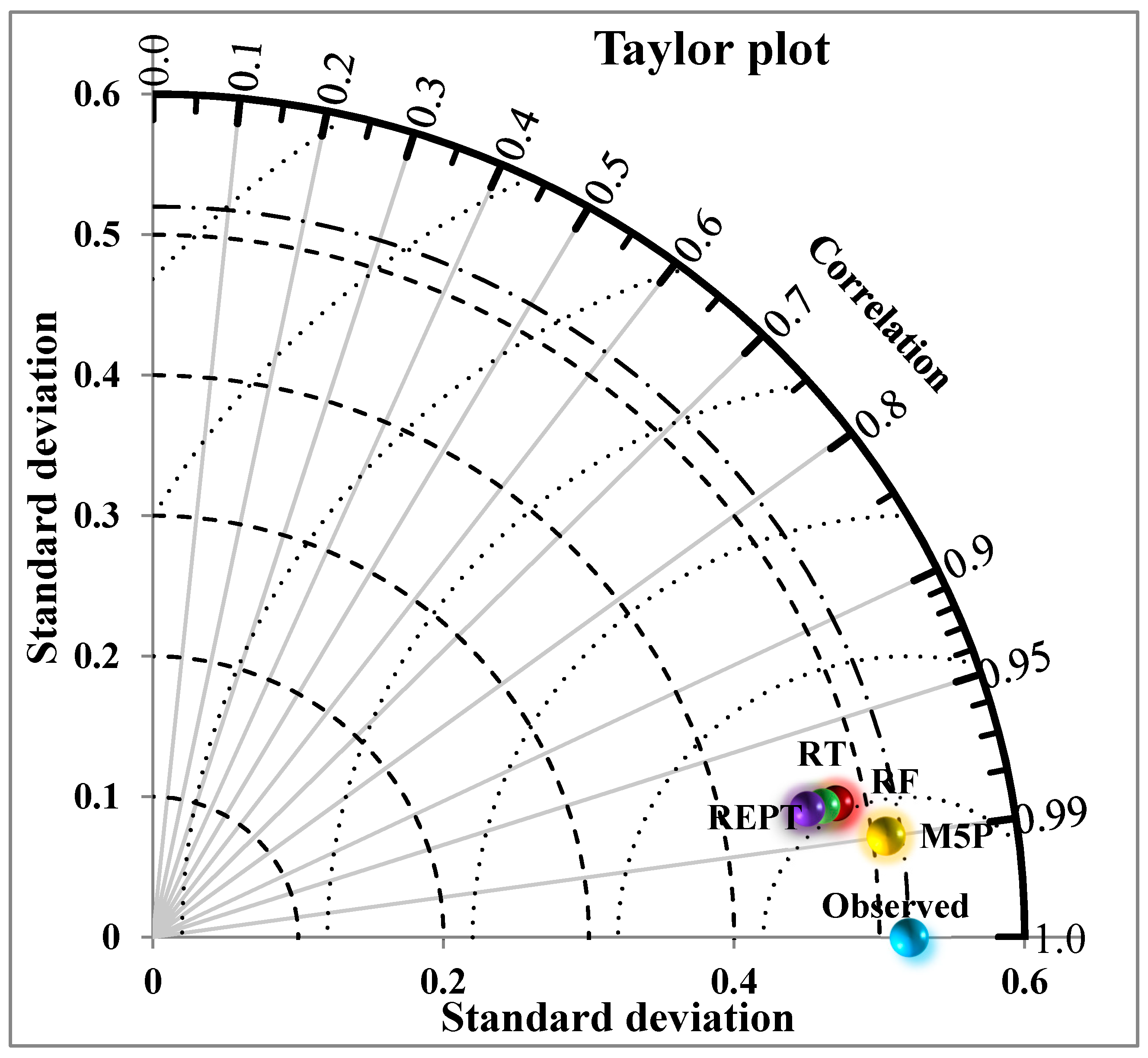
| Models | R2 | RMSE | MAE | NSE | PBIAS | PSR | Order |
|---|---|---|---|---|---|---|---|
| M5P | 0.9874 | 0.05 | 0.01 | 0.98 | 0 | 0.11 | 1 |
| RF | 0.9697 | 0.09 | 0.02 | 0.96 | 0.001 | 0.17 | 2 |
| RT | 0.9654 | 0.09 | 0.03 | 0.96 | 0.001 | 0.19 | 3 |
| REPT | 0.965 | 0.1 | 0.033 | 0.95 | 0.002 | 0.2 | 4 |
| Inputs Variables | WL(t-1) | WL(t-2) | WL(t-3) | WL(t-4) | WL(t-5) |
|---|---|---|---|---|---|
| Correlation coefficient (r) | 0.981 | 0.964 | 0.946 | 0.928 | 0.925 |
| Input Combination No | M5P | RF | RT | REPT | ||||
|---|---|---|---|---|---|---|---|---|
| Train | Test | Train | Test | Train | Test | Train | Test | |
| WL(t-1) | 0.976 | 0.99 | 0.986 | 0.98 | 0.987 | 0.981 | 0.973 | 0.982 |
| WL(t-1), WL(t-2) | 0.976 | 0.993 | 0.991 | 0.978 | 0.994 | 0.961 | 0.973 | 0.977 |
| WL(t-1), WL(t-2) WL(t-3) | 0.979 | 0.993 | 0.991 | 0.979 | 0.994 | 0.961 | 0.972 | 0.982 |
| WL(t-1), WL(t-2), WL(t-3), WL(t-4) | 0.98 | 0.993 | 0.991 | 0.979 | 0.994 | 0.955 | 0.973 | 0.982 |
| WL(t-1), WL(t-2), WL(t-3), WL(t-4), WL(t-5) | 0.978 | 0.993 | 0.991 | 0.98 | 0.994 | 0.963 | 0.973 | 0.982 |
© 2020 by the authors. Licensee MDPI, Basel, Switzerland. This article is an open access article distributed under the terms and conditions of the Creative Commons Attribution (CC BY) license (http://creativecommons.org/licenses/by/4.0/).
Share and Cite
Nhu, V.-H.; Shahabi, H.; Nohani, E.; Shirzadi, A.; Al-Ansari, N.; Bahrami, S.; Miraki, S.; Geertsema, M.; Nguyen, H. Daily Water Level Prediction of Zrebar Lake (Iran): A Comparison between M5P, Random Forest, Random Tree and Reduced Error Pruning Trees Algorithms. ISPRS Int. J. Geo-Inf. 2020, 9, 479. https://doi.org/10.3390/ijgi9080479
Nhu V-H, Shahabi H, Nohani E, Shirzadi A, Al-Ansari N, Bahrami S, Miraki S, Geertsema M, Nguyen H. Daily Water Level Prediction of Zrebar Lake (Iran): A Comparison between M5P, Random Forest, Random Tree and Reduced Error Pruning Trees Algorithms. ISPRS International Journal of Geo-Information. 2020; 9(8):479. https://doi.org/10.3390/ijgi9080479
Chicago/Turabian StyleNhu, Viet-Ha, Himan Shahabi, Ebrahim Nohani, Ataollah Shirzadi, Nadhir Al-Ansari, Sepideh Bahrami, Shaghayegh Miraki, Marten Geertsema, and Hoang Nguyen. 2020. "Daily Water Level Prediction of Zrebar Lake (Iran): A Comparison between M5P, Random Forest, Random Tree and Reduced Error Pruning Trees Algorithms" ISPRS International Journal of Geo-Information 9, no. 8: 479. https://doi.org/10.3390/ijgi9080479