Evaluation of Spatial Resilience of Highway Networks in Response to Adverse Weather Conditions


1
Department of Civil, Construction and Environmental Engineering, The University of New Mexico, MSC01 1070, Albuquerque, NM 87131-0001, USA
2
Earth Data Analysis Center, The University of New Mexico, MSC01 1110, Albuquerque, NM 87131-0001, USA
*
Author to whom correspondence should be addressed.
ISPRS Int. J. Geo-Inf. 2020, 9(8), 480; https://doi.org/10.3390/ijgi9080480
Submission received: 5 June 2020
/
Revised: 22 July 2020
/
Accepted: 29 July 2020
/
Published: 31 July 2020
Abstract
:Adverse weather poses a significant threat to the serviceability of highway infrastructure, as it causes more frequent and severe crash incidents. This study focuses on evaluating the resilience of highway networks by examining the crash-induced safety impact in response to extreme weather events. Unlike traditional service drop-based methods for resilience evaluation, this study endeavors to evaluate highway resilience in a spatial context. Three spatial metrics, including K-nearest neighbors, proximity to highways, and Kernel density hot spot, are introduced and employed to compare and analyze the spatial patterns (magnitude and distribution) of crashes in pre- and post-weather conditions. An illustrative example is also provided to showcase the applications of the proposed spatial resilience metrics for two study areas in the State of Illinois, U.S. The contribution of this study is to provide transportation practitioners with a tool to evaluate highway spatial resilience both visually and quantitatively, and ultimately improve highway safety and operation.
1. Introduction
Highways are vulnerable to adverse weather conditions that pose hazards to motor vehicles and pedestrians and disturb traffic operations (e.g., degraded level of service and roadway closures). The United States highway networks demonstrate certain resilience to weather-related disruptions, including the presence of network redundancy as multiple routes that are often available for long-distance travel, as well as preventative and recovery measures, such as deicing material spreading, weather alerts, and snow/ice removal. When it comes to highway resilience, existing literature focused on quantifying highway network’s service drop in traffic speed and volume, due to various disruptive events such as natural and human-made hazards. However, limited literature has studied highway resilience from the road safety perspective. In this study, the authors develop a new concept of highway resilience—spatial resilience, which focuses on studying the influence of spatial variation of crashes on highway safety to adverse weather conditions. The authors also propose three metrics to spatially measure the safety impact of inclement weather on highway spatial resilience, on the premise that severe weather events result in increased crash rates [1]. These metrics include: (1) K-nearest neighbors (KNN); (2) proximity to highways; and (3) Kernel density hot spot.
The novelty of this research lies in integrating resilience with the spatial patterns shown in traffic crashes—the clustering and distribution of traffic crash incidents in weather-affected areas. This research is expected to provide transportation practitioners with a tool to evaluate highway spatial resilience visually and quantitatively. The proposed spatial metrics can be used to measure highway resilience in terms of weather-related impact on crash patterns, and further investigate non-weather causes of the crashes when different crash attributes (e.g., vehicle speed and road conditions) are taken into account. The manuscript is organized as follows. After reviewing the potential impact of adverse weather on road safety, the authors introduce the concept of spatial resilience in highway safety. Successively, three spatial metrics, along with analysis approaches, are explained in detail prior to demonstrating the applications of the proposed metrics with a case study.
2. Background
2.1. The Resilience of Highway Infrastructure in Adverse Weather
Due to increased frequency and intensity of extreme weather events, highway infrastructure assets in the United States are subject to extensive safety and economic risks, such as fatal crashes and service drop [2]. For instance, severe winter storms could dramatically increase crashes by up to 25 times and reduce road capacity by 12% to 27% [3,4]. The economic loss of degraded services is also substantial. The State of Michigan estimates that the costs of a snowstorm could range from $66 million to $700 million for just a one-day shutdown, due to inaccessible road conditions [2]. In response to the adverse impacts of severe winter storms, in 2014, the U.S. Department of Homeland Security announced the urgent need to study the resilience of critical infrastructure, such as highways to limit the impacts [5].
Resilience for highway systems is often addressed at the network level with regard to how the provision of service alters and restores to a normal state in pre- and post-disruptive events [6]. Under the disruption of winter storms, Nogal et al. [7] examined highway resilience as the network’s capacity to absorb the adverse impacts by identifying different routes for the same pair of origin-destination (O-D) points while minimizing travel costs (i.e., time or money). Adams et al. [8] examined the restoration of highway corridors by tracking truck speed and the number of trucks on the move before and after adverse weather events. In the context of road networks, research on highway resilience has been focused on the assessment of topological and functional performance (e.g., traffic flow and time delay) by simulating and identifying the alternative paths and performance gaps between certain O-D pairs in response to disastrous hazards [9,10,11]. Given the existing literature about highway resilience rarely focus on road safety in terms of the location and geographic proximity of crashes, identifying spatial patterns of crashes represents another vital perspective of highway resilience—spatial resilience.
Besides the service drop, highway networks have demonstrated their vulnerability to severe weather in terms of weather-induced safety hazards to road trips. According to the Federal Highway Administration (FHWA), weather-related crashes are defined as traffic incidents that occur in inclement weather and relevant harsh road conditions [12]. Several researchers concluded that inclement weather events contribute to higher traffic crash rates, a traditional metric for crash analysis [13,14]. Determining the in-depth influence of weather conditions on traffic crash rates can be a multi-variable decision. A simple crash rate, as a ratio of crash count to traffic volume, is insufficient to assess road safety risks [15]. A variety of exposure measures to crash incidents should be considered. The exposure factors (such as speed, time of day, the number of vehicles involved, casualty and injury severity) either serve as reasons for the crashes or can be used to define the crash attributes [15,16].
2.2. Spatial Analysis of Crash Patterns
There are different methods for referencing the locations of crash incidents. One method is that crash incidents can be referenced to road attributes, such as types of road, and the length and width of road segments. For instance, Malin et al. [17] estimated the Palm probability of crash risks that were referenced on different types of road segments (two-lane, multi-lane roads, and motorways) to several weather conditions. Per FHWA guidelines, one of the best practices for detecting traffic incidents is to practice more frequent or enhanced roadway reference markers [18]. In addition to road-related attributes, crashes can be referenced using geographic coordinates (longitude and latitude pair). An advantage of using the geographic coordinates to reference crashes is that the individual crash incidents can be treated as point events in a spatial context which is independent of road networks. This feature prevails when there are no complete highway network datasets which have road centerline data for major highways and arterials but do not include road centerline data for local roads.
The widely-adopted techniques for point-event spatial analysis include: (1) K-nearest neighbor (KNN) approach for pattern classification and forecasting; (2) geostatistical techniques that identify the distribution patterns (e.g., clustering, dispersion, and randomness) of observed data using Moran’s I (both global and local) and Getis-Ord statistics; and (3) Kernel density estimation (KDE) to quantify the level of the probability density for the identified clusters [16]. The KNN method provides a simple but powerful algorithm for recognizing spatial patterns based on Euclidean distance for point events. It classifies a point (traffic crash) into a specific class based on a similarity measure, such as count of neighbors. Wilson et al. [19] used the KNN approach to map the distribution and abundance of multiple tree species over large spatial domains. In the transportation field, researchers expanded the KNN method to develop searching algorithms to forecast traffic state (e.g., vehicle speed) based on previously observed traffic patterns [20,21]. Studying the proximity of point events can examine a typical spatial pattern—clustering, based on the assumption of spatial autocorrelation in which the attributes of one instance at a specific location are affected by the presence of other instances in geographic proximity. Khan et al. [13] adopted Moran’s I and Getis-Ord statistics to identify clustered locations of crashed under snow, rain, and fog weather conditions. Once clustered locations are identified, KDE and its extended Network KDE can be used to illustrate the density level of the contextually related clusters. Hart and Zandbergen [22] examined the performance of different parameter (bandwidth and kernel cell size) settings in KDE to forecast the accuracy of crime hotspots. KDE was also used to identify traffic accident hotspots (regions with high occurrence of crashes) for the classification of road crashes [23]. The outcome of KDE, based on Euclidean distance over planer space, was found to be biased for location datasets over a network space, due to the over-estimation of crash clusters [24]. To overcome this limitation, a network-based KDE was developed and adopted in road network spaces to discern the crash patterns involving different age groups and severity levels [25,26].
3. Spatial Resilience of Highway Networks
In response to weather-related hazards, the existing literature on highway resilience emphasizes attributes related to the level of services (LOS), such as roadway capacity and travel time. In contrast, the safety-related impact has been studied in a separate track via frequency-based statistics or the identification of crash hotspots. Resilience measures that combine the safety and spatial aspects of weather-induced roadway management are infrequently addressed. This research fills the gaps of knowledge in highway resilience by proposing the idea of spatial resilience and its performance metrics that can be used to measure varying crash patterns on highway networks pre- and post-adverse weather events.
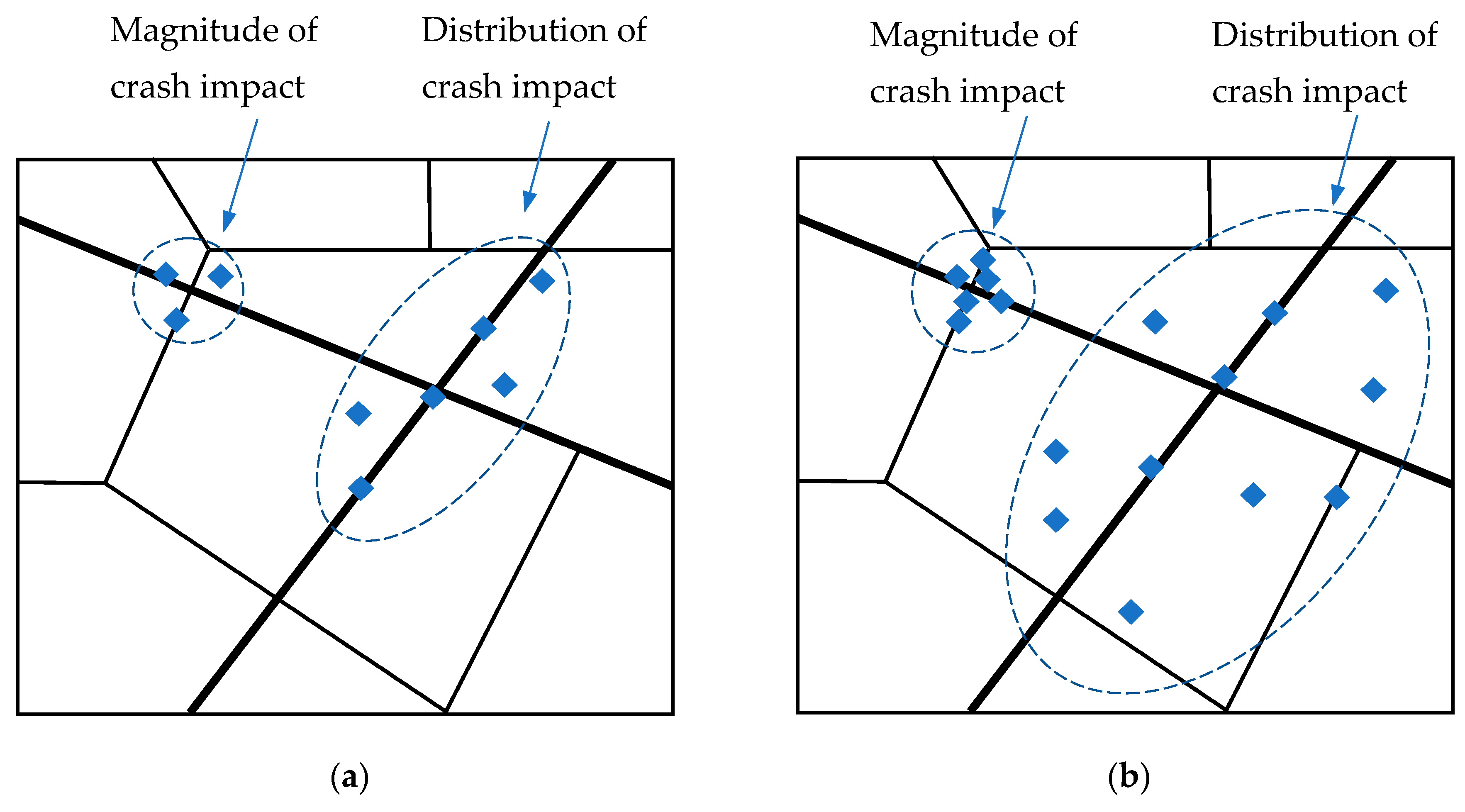
The spatial resilience of a highway network is defined as changes in spatial patterns of crashes in response to extreme weather events. The crash pattern changes capture the ideas of transportation system resilience that measure the system performance variation, due to disruptions and recovery from the disruption to the normal state [6,27]. In this study, an underlying assumption of having a resilient highway network in adverse weather is that the spatial pattern of crashes in adverse weather conditions is expected to remain the same when compared to the crash patterns in non-weather conditions (the “normal” state). Thus, assessing the spatial resilience of highway networks begins with identifying any variations to the crash patterns in adverse weather conditions. When crash pattern variation occurs, the next logical step is to determine how the patterns change in two aspects: magnitude and distribution.
As shown in Figure 1, crash incidents are displayed as points located on either major roads or local roads that exist, but are not shown in the road networks in the same area between pre- and post-weather scenarios. Compared to the crash pattern for the pre-weather scenario in Figure 1a, as the “normal” (baseline) scenario, the authors assume that the number of crashes increases in the post-weather scenario. As shown in Figure 1b, the change in crash patterns means that the crashes could become either more clustered at locations with high crash frequency (magnitude pattern) or extensively spread over a larger area (distribution pattern). From the magnitude perspective, the road network in the post-weather scenario is considered less resilient because the crashes exhibit a more compacted cluster than that of the pre-weather scenario. By contrast, the road network is considered resilient if unchanged or less compacted crash clustering is observed in the post-weather scenario. From the distribution perspective, the road network in the post-weather scenario is also considered less resilient because the crashes are more dispersed than the crash distribution in the pre-weather scenario. On the contrary, the road network is resilient if the crash distribution pattern in the post-weather scenario remains unchanged or becomes less scattered. It is noticeable that the distribution perspective is useful to examine the crash patter changes on local roads whose road centerline data are often incomplete in highway network datasets (e.g., shapefiles). The crash magnitude and distribution serve as the two conceptual elements of the proposed spatial resilience, enabling a fundamental assessment of resilience by detecting highway networks’ vulnerability to weather disruptions [6].
Unlike existing literature that addressed highway resilience in the context of major road networks (e.g., highways and arterials), this research focuses on the geographic location of the crashes. When assessing the spatial patterns of crashes, they do not need to be allocated to a specific major roadway. There are two reasons for this decision. First, crashes could occur on both the major roads or local roads, and omitting the crashes on local roads could lead to non-inclusive spatial patterns. However, a complete and up-to-date road network is not always available, and therefore, focusing on locations instead of road networks will be more accurate for identifying spatial patterns. Second, crashes on local roads may not be in proximity to the ones that occurred on major roads (or at least not in the immediate surrounding areas). Therefore, the authors analyze the spatial resilience of highway networks by investigating the changes in spatial patterns of crash locations within the study areas. In essence, such crash location dataset incorporates three fundamental indicators of spatial relationships in a study area: (1) The count of points in close proximity; (2) the distance from a fixed point to other points or to each other; and (3) the distance from a fixed point to the closest feature (e.g., roadway).
Per the three spatial indicators aforementioned, this research proposes three spatial metrics that can be used to evaluate the spatial resilience of highway networks. It is worth noting that the distance used in the proposed metrics is the Euclidean distance in a planar space rather than the network distance along the roads in a geodetic space. This is because the key to the proposed resilience metrics is to identify the changes in spatial distribution patterns, not traveling times. Additionally, the distance used in the study is relatively short (e.g., 800 m), and therefore, the Earth’s curvature will have a limited impact on the Euclidean distance. The spatial metrics are expected to be able to discern the changes in spatial patterns to indicate how the weather-related safety impact varies from the perspectives of both spatial and temporal scales.
4. Methods
4.1. Data Procedures
Three types of data were required for this research: (1) Geographic area with harsh climate/weather conditions; (2) crash locations; and (3) highway networks in the selected study area. Illinois, a midwestern state in the U.S., was chosen as the target study area because it is often subject to severe winter weather events that pose a threat to road trip safety for the increased crash accident frequency [28]. Two years of crash data in geographic coordinates (2015 and 2016) were obtained from the Illinois Department of Transportation (DOT).
According to National Weather Service [29], adverse winter weather in the State of Illinois includes heavy snow, winter storms, ice storms, and blizzard events. The selected adverse weather days include both weekdays and weekends (a total of 31 days) with the records of the inclement weather events mentioned above from the meteorological winter months in the State of Illinois (December 2015 to February 2016). The same number of weekdays and weekends (31 days) for the non-weather days were also selected within the same timeframe (December 2015 to February 2016), with the aim to obtain a basis of comparison as that of the pre-identified adverse weather days. Then the authors extracted the crash location data (in latitude/longitude format) associated with the two winter weather- and non-weather timeframes.
Given crash characteristics can be quite different on urban and rural roads [30,31], this research specified the Chicago metropolitan area and several counties in the southern part of Illinois separately (in Figure 2) as urban and rural study areas that were affected by the weather events mentioned above. The road network data within the study areas were obtained from the National Highway Planning Networks, the database of the U.S. major highway system which includes national highway routes and principal arterials, and overlaid to the study areas layer with all layers being re-projected in the coordinate system of NAD83 UTM Zone 16N. The number of crash incidents in the Chicago metropolitan area for non-weather and weather scenarios is 15,240 and 19,589, respectively. For the rural county cluster area, the number of crash incidents is 731 (non-weather) and 870 (weather), respectively. These crash data reveal a trend that severe weather will generally cause more crashes [13].
4.2. Spatial Resilience Metrics
4.2.1. K-Nearest Neighbors (KNN)
The authors developed a KNN tool that can be used in a standard GIS software package (Redlands, CA, USA. e.g., ArcGIS). The tool iterates each crash location and uses it as the center point to generate a buffer with a user-defined radius distance (e.g., 200 m), and then selects and counts the crash points that are located entirely within the buffer. The search radii attempted by the authors include the ranges from 100 m to 300 m (with a 50 m incremental interval) for urban areas and the ranges from 800 m to 1000 m (with a 100 m incremental interval) for rural areas, by following the distance thresholds recommended by Thakali et al. [16] and Ulak et al. [26]. The results (in K percentage values) present the counts of adjacent crashes to a specific crash location in different cluster groups. The KNN tool is used to examine crash pattern variation in terms of crash magnitude—one spatial resilience indicator for highway networks. As mentioned above, the critical assumption of having a resilient highway network in adverse weather conditions is that the crash pattern in adverse weather conditions remains the same as the pattern in non-weather conditions (or “normal” state). The KNN results are used to identify if there are changes in clustering patterns between non-weather and weather conditions. If the pattern does change, the KNN outputs can then be used to investigate if the crashes become more clustered in adverse weather conditions. The resultant percent changes in the specified cluster groups show the clustering pattern shift between the non-weather and weather scenarios in a qualitative way. Specifically, the authors interpret the percent change in each cluster group as “increased,” “decreased,” or “no obvious changes”, and then examine if a certain percentage of crash shifts from no cluster to different cluster groups. Eventually, the overall trend of the pattern shift across all the cluster groups can be summarized. When the crashes in adverse weather conditions become more clustered, then the magnitude of safety impact increases—indicating less resilient highway networks. In contrast, the highway networks are considered resilient to the weather conditions if the crashes turn out to be less clustered or remain unchanged.
4.2.2. Proximity to Highways
The second proposed metric for measuring spatial resilience of highway networks is proximity to highways, which considers the situation that some crashes occurred on local roads but not on highways networks. This metric can be used to measure if weather-impacted crashes have similar proximity to highways as the non-weather impacted crashes—the spatial distribution of crash impact, which represents the other spatial resilience indicator in this research. In the context of disruptive events (adverse weather conditions), a resilient highway network should preserve crashes’ proximity patterns to highways (i.e., crash distribution pattern in normal non-weather conditions) rather than vary dramatically. For example, a highway network would be less resilient if the post-weather crash locations exhibit a different proximity pattern (e.g., more widespread crashes) from the pre-weather crash locations. By contrast, the highway networks are resilient if no proximity pattern shift is observed between the pre- and post-weather scenarios. Proximity to highways analysis was achieved through the use of point-to-polyline overlay analysis, and more specifically, through measuring the distance from crash points to the nearest highway centerline. A cumulative distribution function (CDF) was then developed to assess how well the post-weather crash locations approximate the pre-weather crash locations. When creating the CDF, each location was considered to have an equal percentage and then sorted by the shortest distance to the longest distance. When interpreting the CDF graph, more disparities indicate less resilience. It should be noted that distance is calculated based on the Euclidean distance from the crash points to the nearest highways but not the entire road network (i.e., excluding local roads). This is because this metric is designed to analyze if the pre-weather crash locations exhibit a similar proximity pattern as the post-weather crash locations, and therefore, which road network is being in use is irrelevant.
4.2.3. Hotspot Analysis Based on Kernel Density Estimation (KDE)
The third metric for measuring spatial resilience involves evaluating the magnitude and distribution of the hotspots of crash locations. Crash clustering and distribution are dependent on spatial scales. Within a cluster of crashes, each individual crash can be considered as being far apart from each other (distribution effect). In contrast, widespread crashes (e.g., crashes occurred around major highways) can be treated as a single cluster for road safety assessment at a large spatial scale (e.g., highway networks and their surrounding spaces). So, crash hotspots are established to represent a combined effect of both magnitude and distribution of crash impact. The size of crash hotspots (areas) is used as an indicator of highway spatial resilience. Compared to pre-weather crash hotspots, post-weather crash hotspots that cover an extensive area suggest less resilient road networks being involved, indicating both increased clustering magnitude and extended distribution of crash impact.
The KDE approach, a non-parametric density estimation technique, is utilized because it can provide not only a visual presentation of crash hotspots and their temporal changes, but also a quantitative measurement of the size of hotspots and their temporal changes [32]. The selection of searching bandwidth and kernel size, the two primary parameters for KDE, can be a subjective process [23,33]. In this research, the authors used the bandwidths which were recommended by existing research about crash hotspot analysis, including 100 m in the urban (Chicago metropolitan) areas [34] and 800 m in rural (southern Illinois counties) areas [20], respectively. The selection of kernel size is a trade-off between the computation time and crash information to retain as long as discernable crash clustering patterns can be identified [16]. For output pixel size, 50 m was used, resulting in a pixel area of 2500 square meters (m2). The chosen kernel size of 50 m is considered appropriate because the crash clustering pattern (hotspot) variations can be observed between the pre- and post-weather scenarios. The output hotspot maps were presented in the raster data format consisting of a grid of pixels whose values represent Kernel density levels. Based on the calculated mean density value, the output density values were reclassified into different categories [22]. Each category represents a range of pixel values that are equal to the mean density value multiplied by a sequence of positive integers (e.g., 1, 2, 3, 4, and 5) until the largest output pixel values can be included. Since there are no established rules for defining hotspots, finding the hotspots is a rather arbitrary decision—generally selecting a cutoff point of density values to determine clusters across the studied density surface [16]. In this study, a hotspot is defined as a group of pixels that have density values at least five times greater than the mean density value. This selection was based on the observation of the case study data, which could be different for another study area. Ultimately, the hotspot areas can be computed by multiplying a single-pixel size (2500 m2) by the total number of hotspot pixels.
5. Results
This section showcases how the proposed metrics can be used to evaluate the spatial resilience of highway networks in the scenarios of pre- and post-snowstorm weather events. The focus of the proposed metrics is to investigate if crash patterns change in adverse weather conditions. The expected results are explanatory for transportation agencies like DOTs or local governments to evaluate the safety aspect of highway resilience at the city and regional levels in response to inclement winter weather events, which indirectly assists with the decision-making on corresponding road weather management practices, such as alternative routes mapping and snow/ice removal.
5.1. KNN
The KNN analysis was performed for the crashes located in the Chicago metropolitan and rural county areas affected by the adverse weather in the winter of 2015 and 2016. The output “K” refers to the count of adjacent crashes to a specific crash location. It is observed from a visual check of the crash location maps that the crash pattern changes between the non-weather (N-W), and storm weather (W) scenarios are subtle. To look into the slight pattern changes, the authors present the output “K” in several bins (cluster groups), including K = 0 (no cluster), 1 ≤ K ≤ 5 (small clusters), 5 < K ≤ 10 (medium clusters), K > 10 (large clusters), as shown in Table 1 and Table 2. Each bin has the corresponding K outcomes comparing the N-W and W scenarios at different search radii. The results (percent of KNN for each bin) can be used to examine changes in crash clustering patterns, therefore suggesting the magnitude of the safety impact of adverse weather events.
For the Chicago metropolitan area (Table 1), the results at the search radius of 100 m show that the no-cluster case declines (from 46.69% to 43.95%) in the W scenario, suggesting an increasing trend of clustering that shifts to the different cluster groups even if this pattern shift is slight. The small clusters (1 ≤ K ≤ 5) case increases approximately by 2% from 46.42% to 48.43%, and a minor percent increase also occurs to the large clusters (K > 10) case. For the medium clusters (5 ≤ K ≤ 10), the percent change between the N-W and W scenarios is too minor to be distinguishable (5.49% vs. 5.45%). In this case, the authors conclude that the crashes along the magnitude of the crash impact tend to intensify in the Chicago metropolitan area as the small percent of crashes shifts from the no-cluster case to the small and large cluster groups. A similar trend is observed from the results of a sensitivity analysis when using the search radii of 150 m and 200 m. Given the high density of traffic and road facilities in Chicago, the minor increase of crash clustering can be substantial in terms of the actual number of crashes this growth could represent. So, this minor clustering growth could suggest a far-reaching safety impact and its ripple effect on the highway network and its surrounding spaces where local roads are located. Hence, the studied highway networks in the Chicago metropolitan area are considered less resilient in response to the storm weather events.
Compared to the urban areas, the KNN results for rural county clusters display less consistent crash patterns. Three search radii (800 m, 900 m, and 1000 m) were applied, given the lower density of traffic and road facilities in the rural areas. When using a radius of 800 m, the discernable percent changes can be observed from the small and medium cluster groups but go in a different direction. The small cluster group (1 ≤ K ≤ 5) shows a 5.02% increase (from 39.12% to 44.14%), while the medium cluster group (5 < K ≤ 10) drops by 4.05% (from 8.76% to 4.71%) in the W scenario. Another percent drop is observed from the large cluster group (K > 10) from 2.74% to 2.07% (0.67% decrease). For the no cluster group, the percent also declines from the N-W to W scenario, but the difference is minor (49.38% vs. 49.08%). A similar trend is also observed from the KNN results (except for the no cluster group which shows a slight increase in the W scenario) based on the search radii of 900 m and 1000 m. For the inconsistent trend of crash pattern shifts between different cluster groups, it is inadequate to evaluate the overall trend of clustering patterns by comparing the percent changes only due to the “zero-sum” effect for the percent increase and decrease between the cluster groups. Instead, the authors argue that the specified cluster groups can be used to assess the different magnitude of crash clustering (e.g., the medium cluster group has a greater magnitude of clustering than the small cluster group). Thus, the overall trend of crash clustering is considered diminished since the two (medium and large) out of three cluster groups show the declined percent of the corresponding crash clusters in the W scenario, suggesting that the highway networks in rural counties are resilient to the adverse weather conditions.
5.2. Proximity to Highways
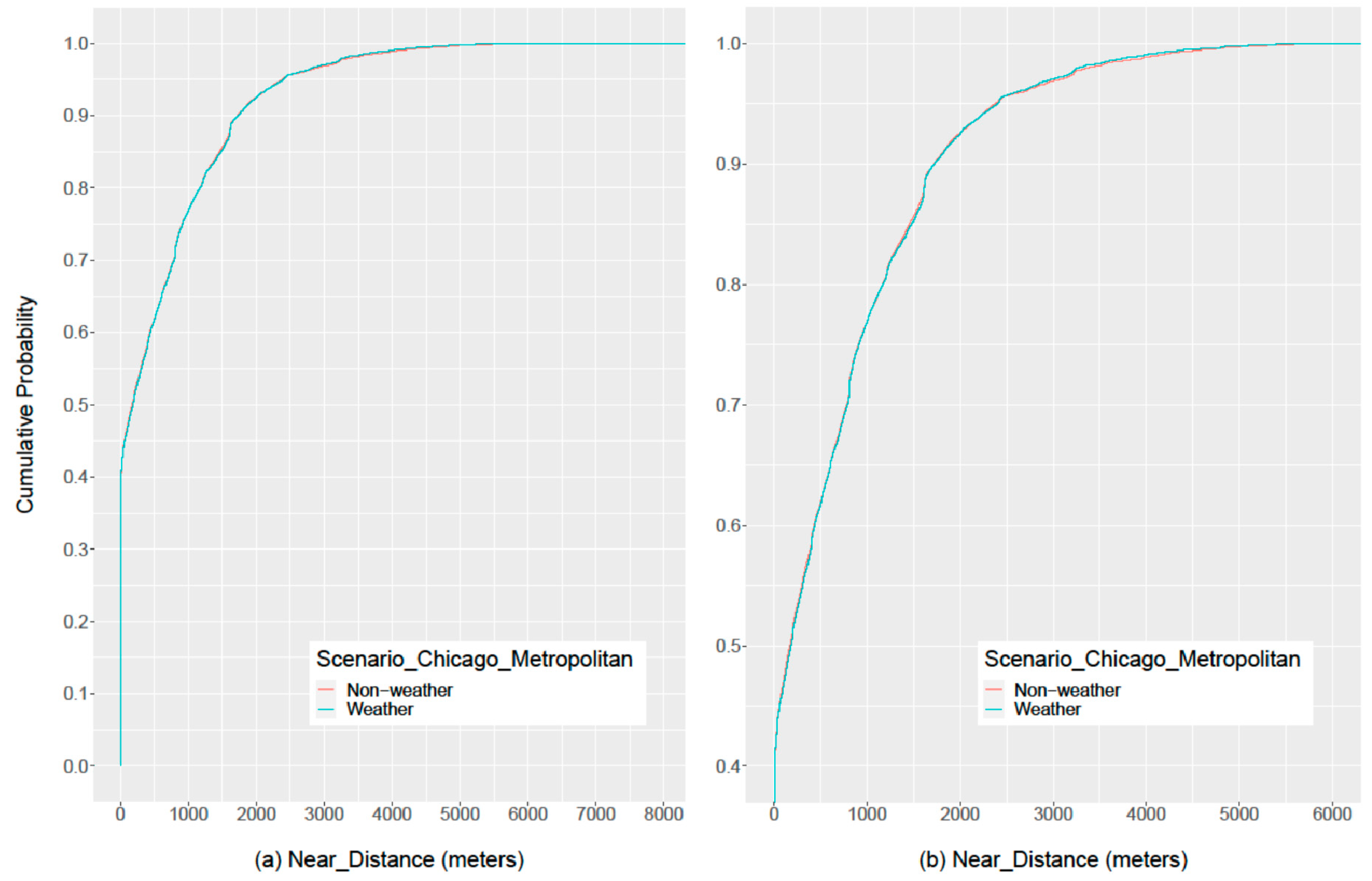
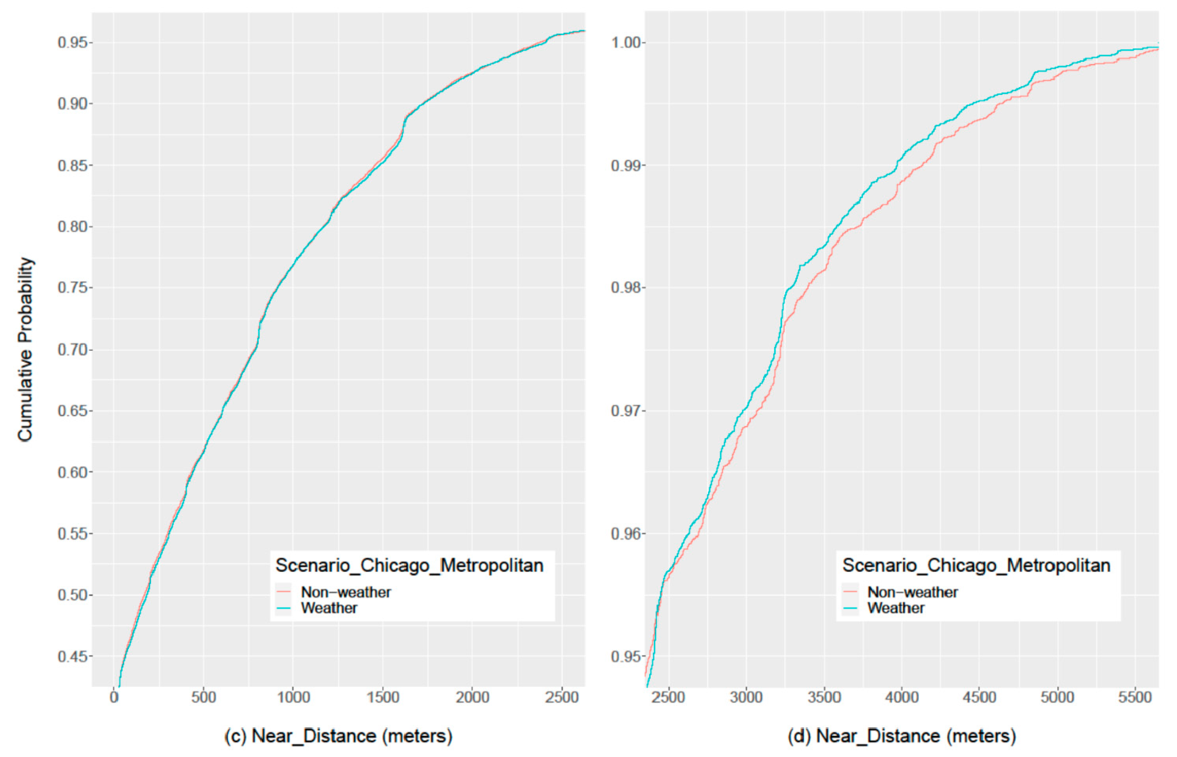
For the same study areas, the authors conducted point-to-polyline analyses and developed corresponding CDF graphs. Figure 3 and Figure 4 show the outcomes in the CDF graphs to exhibit how crashes are distributed away from the major highways.
In the Chicago metropolitan area, the outputs of the proximity to highways analysis indicate that about 43% of the observed crashes occurred on major highways, which is equal to 6553 (15,240 × 43%) and 8423 (19,589 × 43%) crashes for the N-W and W scenarios, respectively. The on-highway crashes are identified if their locations to the nearest highway centerlines are equal or less than 32 m (maximum width of seven-lane highways in Chicago areas). The remaining 57% of the crashes on local roads (8687 and 11,166 crashes for the N-W and W scenarios) are used to examine the crash distribution patterns related to but not on the highway networks. By setting labeling limits on the axes, the authors present several zoom-in displays in Figure 3b–d to identify how the crashes disperse away from the major highways between the N-W and W scenarios. At first glance, the crashes off the major highways do not show clear pattern changes between the two scenarios in Figure 3b. This case could be partly because the road networks are dense in urban areas and include many local roads that either in parallel (e.g., frontage roads) or connected to the major highways. However, slight pattern shifts are observed at certain ranges of the nearest distances. In Figure 3c, the non-weather line is slightly above the weather line between 100–500 m and 1250–1600 m, indicating that within these ranges of distance, say 250 m to the nearest highway, there are slightly more crashes under non-weather conditions than those under weather conditions. This pattern implies that crashes tend to spread a little further from the major highways on severe weather days. Per Figure 3d, a reversed pattern is noticed between 2500–5500 m to the nearest highways where more crashes in the W scenario are observed than those in the N-W scenario. Given the minor pattern shift (less than 1% cumulative probability) between the two scenarios, there is no distinct dispersion of the crashes away from the adjacent highway networks. Hence, the results cannot prove that the highway networks are resilient to the adverse weather, using the resilience indicator that measures the distribution of the crashes around the major highways.
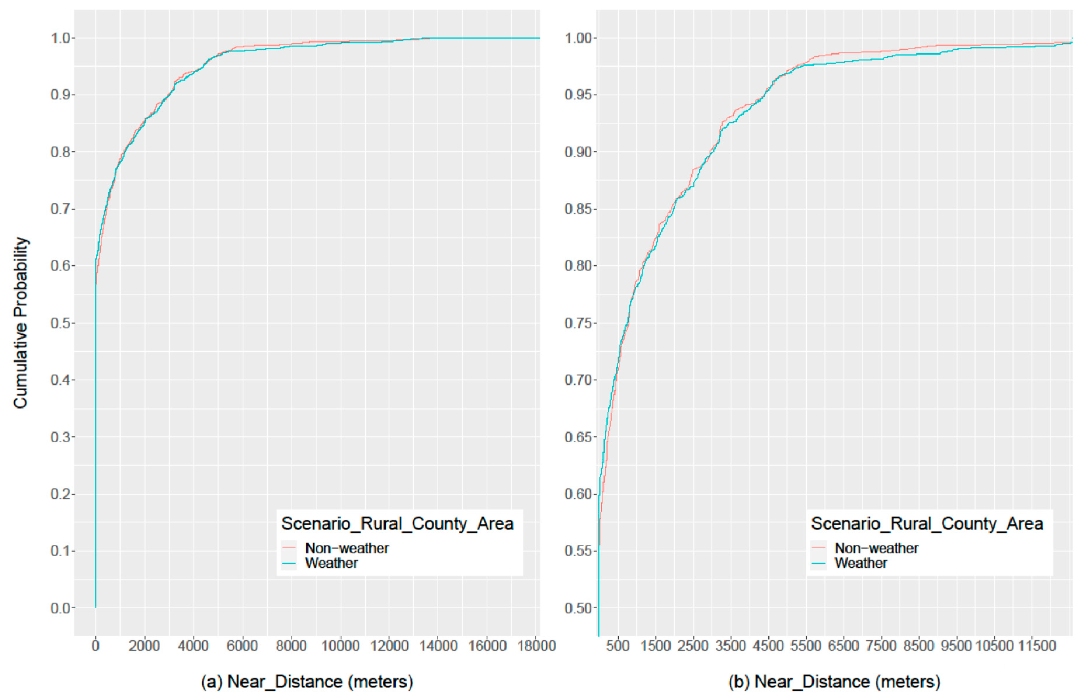
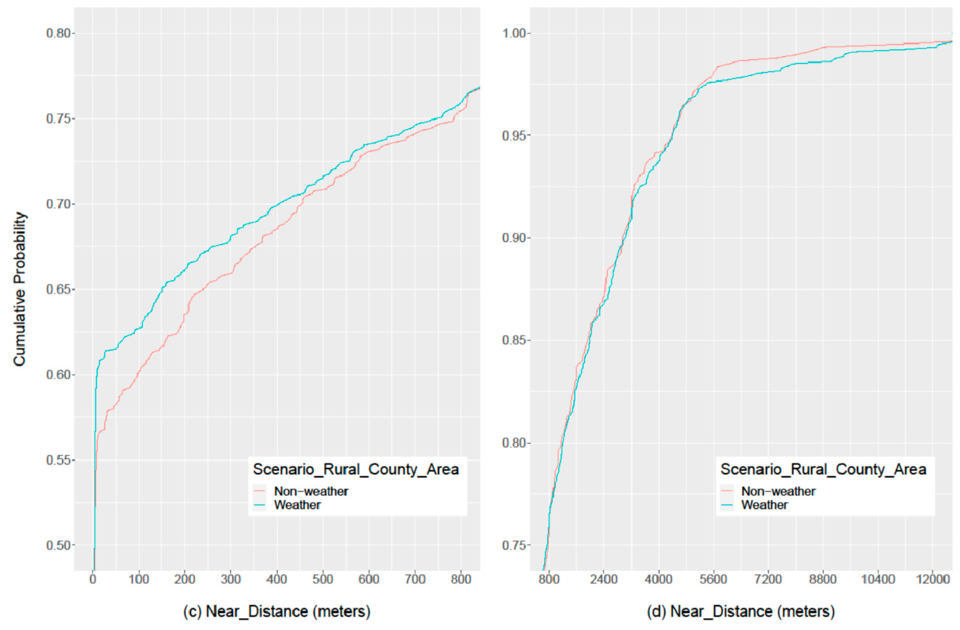
For the rural county clusters, the crashes on major highways account for about 56% (731 × 56% = 409 crashes) and 60% (870 × 60% = 522 crashes) of the total crashes for the N-W and W scenarios. Unlike the Chicago metropolitan area, the on-highway crashes are determined if the locations to the nearest highway centerlines are equal or less than 11 m (maximum width of two-lane highways in the studied rural counties). To identify the crash distribution patterns, the authors looked into the portion of the off-highway crashes 44% (322 crashes) for the N-W scenario and 40% (348 crashes) for the W scenario. Figure 4a,b show that the pattern shift appears between the two scenarios from the cumulative percentage of 56%, and therefore, varies over distance. For the crashes that happened far away from the major highways (800–12000 m) in Figure 4d, no distinct pattern shifts are observed between the two scenarios as the two lines are interleaved and trending up from 75% all the way to 97%. Thereafter, the crashes for the N-W scenario tend to remain closer to the major highways than those for the W scenario. However, this pattern shift is not substantial as only 3% of the total crashes (from 97% toward 100%) are involved. For the crashes that occurred near the major highways, say up to 800 m, shown in Figure 4c, the percent of the crashes for the W scenario is continuously higher than that of the N-W scenario, which indicates that in this distance range, the crashes in the context of severe weather tend to be in close proximity to the major highways. For instance, at a cumulative probability of 65%, the crashes in the W scenario occurred at no further than 150 m away from the major highways while the crashes in the N-W scenario occurred as far as 250 m to the major highways. This proximity pattern suggests that the corresponding safety impact under the extreme weather condition is less dispersed than that of the normal condition. Thus, the highway networks in the rural county clusters are considered spatially resilient in response to weather disruptions. This situation could be partly because the road conditions on the major highways in rural areas are better than the local roads, due to timely snow/ice removal, which pushes the traffic toward the major highways.
5.3. Hotspots Based on KDE
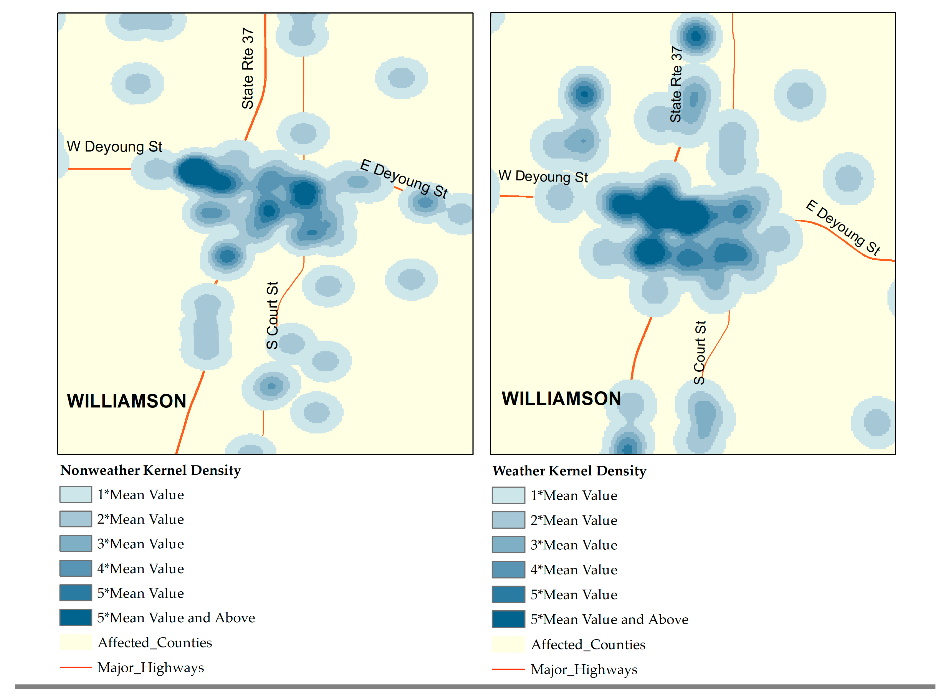
This section demonstrates the use of the KDE analysis to identify hotspots for the rural county clusters. The resultant hotspot area located in Williamson county is chosen to showcase how to examine spatial resilience of the highway networks involved using the KDE results, including (1) a kernel density map that visualizes crash hotspots and their immediate surrounding spaces; (2) quantification of the size of the hotspots. Figure 5 shows the Kernel density map to compare crash hotspots between the weather and non-weather scenarios. The legends in the density map highlight the crash-prone zones estimated based on the number of crashes over a specified grid with a cell size of 50 m. As shown in the maps, the crash pattern shifts can be visually detected on the highway networks, as well as the local roads. The hotspot in the W scenario is larger than that in the N-W scenario. It is worth noting that the identified crash clusters by the planar KDE cover the area for the crash locations and the immediate surrounding spaces within the search bandwidth (800 m).
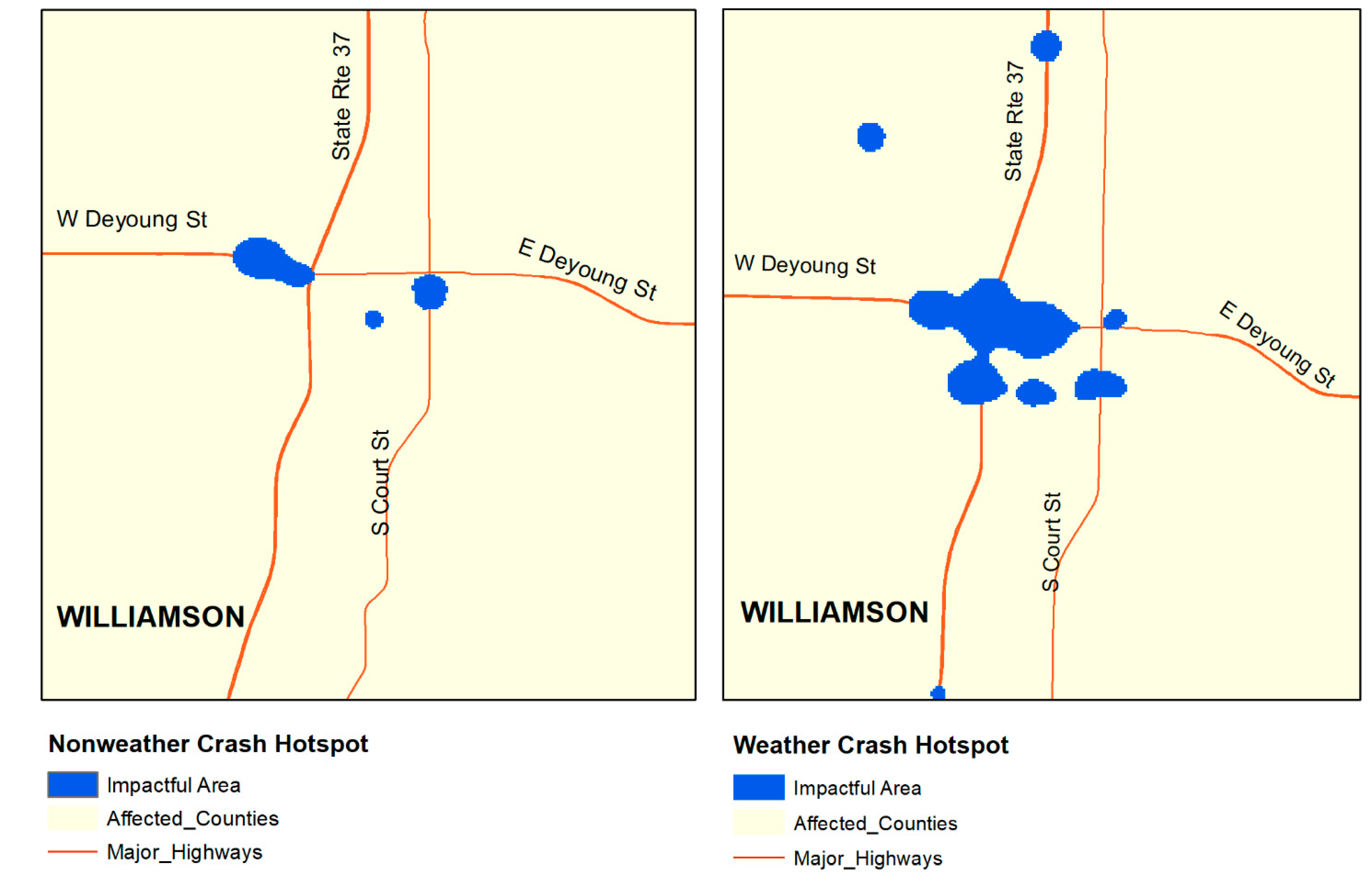
The crash clusters with relatively high-density values are considered the impactful area (hotspots) from the spatial resilience perspective, suggesting extended magnitude and distribution of crash impact. Based on the calculated mean density value of all pixels, the authors reclassified the density values into six classes ranging from 100%, 200%, 300%, 400%, 500%, and above of the mean density value. The cells with density values that fall under five times mean value and above of all pixels are considered to be hotspots. In this case, the reclassify analysis was performed over the entire study area to generate hotspot maps in the non-weather and weather scenarios. Still using the crash clusters in the Williamson county as an example, the pre-defined density classes (500% and above of the average density) are combined and presented in one color scheme, as shown in Figure 6. For the W scenario, the area of the identified crash hotspots appears larger than that of the N-W scenario, suggesting that the impactful area (hotspot) of the crashes intensifies in adverse weather conditions. To quantify the impactful areas, the authors exported the number of cells associated with the crash hotspots for the entire study area, as shown in Table 3.
For the N-W scenario, the impactful area consists of 5502 cells, which is an equivalent of 13.755 km2. In adverse weather conditions, the impactful area fills up 7795 cells and reaches up to 19.4875 km2, with an increase of 42%. This outcome indicates that adverse weather conditions influence the spatial resilience of highway networks as far as road safety concerns. For the hotspots detected in the two scenarios, the increased impactful areas show that the magnitude of safety impact of adverse weather conditions grows as there are increased number of the crashes occurred at the hotspots in adverse weather conditions, and therefore, the corresponding highway networks are considered less resilient to those spots (e.g., the one in the Williamson county). The same rationale applies to the overall study area when the impactful areas are grouped together (in Table 3). Meanwhile, the increased impactful area also illustrates a more extensive distribution of the safety impact caused by the crash hotspots—the other attribute of spatial resilience proposed in this research. Consequently, the selected portion of highway networks in Williamson county is considered less resilient in response to the adverse weather.
6. Discussions
The KNN metric measures the magnitude of crash-related safety impact in adverse weather conditions by uncovering a latent spatial pattern that if the crashes tend to become clustered. The degree of clustering (K value) can be used to investigate various underlying issues for highway operation (e.g., road slipperiness and insufficient super-elevation) and entail contingent measures specific to the study areas. The proximity to highways addresses the distribution of crash-related safety impact in adverse weather conditions, especially for the crashes occurred on the local roads, which is non-negligible, although oftentimes the local roads are not included in the available databases of highway networks. The further those crashes distribute away from the major highways, the higher safety impact exhibits, and subsequently, the corresponding segments of the highway networks are considered less resilient. Lastly, the impactful area based on the KDE analysis is inclusive of both magnitude and distribution of safety impact and visually presents how temporal patterns change. The resultant density maps allow users to define a crash hotspot based on density values and then examine if and how the safety impact spreads. The spread counts the impactful area of the crashes on the highways and local roads. The quantifiable impactful areas are intended to provide safety and planning professionals a safety performance indicator that can be used to monitor the weather-induced impact on crash-prone highway segments and their surrounding spaces.
The findings of this research are considered meaningful to the investigation of weather influence on road safety from two aspects: (1) Exploring crash pattern changes between the non-weather and weather scenarios. The pattern changes serve as alternative metrics that can be used to evaluate road safety in addition to the traditional frequency- and severity-based metrics. The proposed spatial metrics support the safety vulnerability detection as the outcome comes with numeric indicators to inform decision-makers on the pattern changes that are too subtle to be visually detected from traditional mapping solutions; (2) providing insights into the distribution of crash impact in response to extreme weather conditions. With the proximity to highways and impactful area analysis, transportation practitioners can speculate, from the quantitative pattern shifts, the potential interactions between major highways and local roads, even though oftentimes the local roads are not included in most highway network databases. For instance, the proximity to highways could be useful to evaluate the effectiveness of recovery measures (e.g., ice/snow removal) during and after severe weather events. In this study, major highways are assumed to carry the majority of traffic while the traffic on local roads is either diverging from the highways or converging to the highways. If no substantial volume change is detected between non-weather and weather scenarios, the crash distribution (via proximity to highways metric) in adverse weather conditions indicates if the major highways can hold the traffic volume as normal, or otherwise, the traffic on the highways get partially distributed to the local roads.
7. Conclusions
For the increasing risk of inclement weather, this research relates the resilience of highway infrastructure to road safety in a weather-impacted perspective. Unlike existing resilience metrics that focus on the highway performance drop, the authors examined the characteristics of crashes’ locational data and defined resilience based on two spatial attributes obtained from the crash data: The magnitude and distribution of the safety impact. Accordingly, three metrics (KNN, proximity to highways, and the impactful area based on KDE) are proposed for the spatial resilience assessment. The proposed metrics for spatial resilience analysis are intended to evaluate the crash pattern shift between the non-weather and weather scenarios, which is illustrated in the previous case study The pattern shifts indicate the resilience status of highway networks; the more intense and or widespread the crash clustering becomes, the less resilient the affected road networks are.
The outcomes from the proposed resilience metrics are explanatory, but providing the indicators to public agencies like state DOTs who will determine the causal relationships between the preventative/recovery measures and resulting crash risks. Moreover, resilience measured from the safety aspect contributes to the ‘big picture’ of resilience assessment for highway infrastructure by introducing future research needs. For instance, the effectiveness of the spatial resilience metrics needs to be verified by existing metrics of highway resilience related to the performance drop. The combined results are valuable to practitioners for guiding the safety and winter road management programs. Moreover, the spatial resilience metrics could be specified and developed by considering exposure factors to crash risks involved, such as the specific types of crashes or weather events.
Author Contributions
Conceptualization, Fei Han; Methodology, Fei Han and Su Zhang; Software, Fei Han and Su Zhang; Validation, Fei Han and Su Zhang; Formal Analysis, Fei Han and Su Zhang; Investigation, Fei Han; Resources, Fei Han and Su Zhang; Data Curation, Fei Han and Su Zhang; Writing—Original Draft Preparation, Fei Han; Writing—Review & Editing, Fei Han and Su Zhang; Visualization, Fei Han and Su Zhang; Project Administration, Fei Han. All authors have read and agreed to the published version of the manuscript.
Funding
This research received no external funding.
Acknowledgments
The authors thank the Illinois Department of Transportation, U.S. for providing the crash data that greatly assisted the research.
Conflicts of Interest
The authors declare no conflict of interest.
References
- Qiu, L.; Nixon, W.A. Effects of adverse weather on traffic crashes: Systematic review and meta-analysis. Transp. Res. Rec. 2008, 2055, 139–146. [Google Scholar] [CrossRef]
- Meyer, M.D.; Rowan, E.; Snow, C.; Choate, A. Impacts of Extreme Weather on Transportation: National Symposium Summary; American Association of State Highway and Transportation Officials: Washington, DC, USA, 2013. [Google Scholar]
- Maze, T.H.; Agarwal, M.; Burchett, G. Whether weather matters to traffic demand, traffic safety, and traffic operations and flow. Transp. Res. Rec. 2006, 1948, 170–176. [Google Scholar] [CrossRef]
- FHWA, Federal Highway Administration. How Do Weather Events Impact Roads? 2014. Available online: https://ops.fhwa.dot.gov/weather/q1_roadimpact.htm (accessed on 25 February 2020).
- OCIA. Critical Infrastructure Security and Resilience Note: Winter Storms and Critical Infrastructure. 2014. Available online: http://www.npstc.org/download.jsp?tableId=37&column=217&id=3277&file=OCIA_Winter_Storms_and_Critical_Infrastructure_141215.pdf (accessed on 17 February 2020).
- Machado-León, J.L.; Goodchild, A. Review of Performance Metrics for Community-Based Planning for Resilience of the Transportation System. Transp. Res. Rec. 2017, 2604, 44–53. [Google Scholar] [CrossRef]
- Nogal, M.; O’Connor, A.; Martinez-Pastor, B.; Caulfield, B. Novel probabilistic resilience assessment framework of transportation networks against extreme weather events. ASCE-ASME J. Risk Uncertain. Eng. Syst. Part A Civ. Eng. 2017, 3, 04017004. [Google Scholar] [CrossRef]
- Adams, T.M.; Bekkem, K.R.; Toledo-Durán, E.J. Freight resilience measures. J. Transp. Eng. 2012, 138, 1403–1409. [Google Scholar] [CrossRef]
- Ganin, A.A.; Kitsak, M.; Marchese, D.; Keisler, J.M.; Seager, T.; Linkov, I. Resilience and efficiency in transportation networks. Sci. Adv. 2017, 3, e1701079. [Google Scholar] [CrossRef] [Green Version]
- Woodburn, A. Rail network resilience and operational responsiveness during unplanned disruption: A rail freight case study. J. Transp. Geogr. 2019, 77, 59–69. [Google Scholar] [CrossRef]
- Zhang, X.; Miller-Hooks, E.; Denny, K. Assessing the role of network topology in transportation network resilience. J. Transp. Geogr. 2015, 46, 35–45. [Google Scholar] [CrossRef] [Green Version]
- Pisano, P.A.; Goodwin, L.C.; Rossetti, M.A. US highway crashes in adverse road weather conditions. In Proceedings of the 24th Conference on International Interactive Information and Processing Systems for Meteorology, Oceanography and Hydrology, New Orleans, LA, USA, 20–24 January 2008. [Google Scholar]
- Khan, G.; Qin, X.; Noyce, D.A. Spatial analysis of weather crash patterns. J. Transp. Eng. 2008, 134, 191–202. [Google Scholar] [CrossRef]
- Andrey, J. Long-term trends in weather-related crash risks. J. Transp. Geogr. 2010, 18, 247–258. [Google Scholar] [CrossRef]
- Qin, X.; Ivan, J.N.; Ravishanker, N. Selecting exposure measures in crash rate prediction for two-lane highway segments. Accid. Anal. Prev. 2004, 36, 183–191. [Google Scholar] [CrossRef]
- Thakali, L.; Kwon, T.J.; Fu, L. Identification of crash hotspots using kernel density estimation and kriging methods: A comparison. J. Mod. Transp. 2015, 23, 93–106. [Google Scholar] [CrossRef] [Green Version]
- Malin, F.; Norros, I.; Innamaa, S. Accident risk of road and weather conditions on different road types. Accid. Anal. Prev. 2019, 122, 181–188. [Google Scholar] [CrossRef] [PubMed]
- Carson, J.L. Best Practices in Traffic Incident Management (No. FHWA-HOP-10-050); Federal Highway Administration, Office of Transportation Operations: Washington, DC, USA, 2010. [Google Scholar]
- Wilson, B.T.; Lister, A.J.; Riemann, R.I. A nearest-neighbor imputation approach to mapping tree species over large areas using forest inventory plots and moderate resolution raster data. For. Ecol. Manag. 2012, 271, 182–198. [Google Scholar] [CrossRef]
- Oh, S.; Byon, Y.J.; Yeo, H. Improvement of search strategy with k-nearest neighbors approach for traffic state prediction. IEEE Trans. Intell. Transp. Syst. 2015, 17, 1146–1156. [Google Scholar] [CrossRef]
- Cai, P.; Wang, Y.; Lu, G.; Chen, P.; Ding, C.; Sun, J. A spatiotemporal correlative k-nearest neighbor model for short-term traffic multistep forecasting. Transp. Res. Part C Emerg. Technol. 2016, 62, 21–34. [Google Scholar] [CrossRef]
- Hart, T.; Zandbergen, P. Kernel density estimation and hotspot mapping. Policing: An International J. Police Strateg. Manag. 2014, 37, 305–323. [Google Scholar] [CrossRef]
- Anderson, T.K. Kernel density estimation and K-means clustering to profile road accident hotspots. Accid. Anal. Prev. 2009, 41, 359–364. [Google Scholar] [CrossRef]
- Xie, Z.; Yan, J. Detecting traffic accident clusters with network kernel density estimation and local spatial statistics: An integrated approach. J. Transp. Geogr. 2013, 31, 64–71. [Google Scholar] [CrossRef]
- Lee, M.; Khattak, A.J. Case study of crash severity spatial pattern identification in hot spot analysis. Transp. Res. Rec. 2019, 2673, 684–695. [Google Scholar] [CrossRef]
- Ulak, M.B.; Ozguven, E.E.; Spainhour, L.; Vanli, O.A. Spatial investigation of aging-involved crashes: A GIS-based case study in Northwest Florida. J. Transp. Geogr. 2017, 58, 71–91. [Google Scholar] [CrossRef]
- Linkov, I.; Bridges, T.; Creutzig, F.; Decker, J.; Fox-Lent, C.; Kröger, W.; Nyer, R. Changing the resilience paradigm. Nat. Clim. Chang. 2014, 4, 407. [Google Scholar] [CrossRef]
- Theofilatos, A.; Yannis, G. A review of the effect of traffic and weather characteristics on road safety. Accid. Anal. Prev. 2014, 72, 244–256. [Google Scholar] [CrossRef]
- National Weather Service. Available online: https://www.weather.gov/ (accessed on 17 February 2020).
- Li, M.D.; Doong, J.L.; Chang, K.K.; Lu, T.H.; Jeng, M.C. Differences in urban and rural accident characteristics and medical service utilization for traffic fatalities in less-motorized societies. J. Saf. Res. 2008, 39, 623–630. [Google Scholar] [CrossRef] [PubMed]
- Zwerling, C.; Peek-Asa, C.; Whitten, P.S.; Choi, S.W.; Sprince, N.L.; Jones, M.P. Fatal motor vehicle crashes in rural and urban areas: Decomposing rates into contributing factors. Inj. Prev. 2005, 11, 24–28. [Google Scholar] [CrossRef]
- Silverman, B.W. Density Estimation for Statistics and Data Analysis; CRC press: Boca Raton, FL, USA, 1986; Volume 26. [Google Scholar]
- Levine, N. CrimeStat III: A Spatial Statistics Program for the Analysis of Crime Incident Locations (Version 3.0); Ned Levine & Associates: Houston, TX, USA; National Institute of Justice: Washington, DC, USA, 2004.
- Pulugurtha, S.S.; Vanapalli, V.K. Hazardous bus stops identification: An illustration using GIS. J. Public Transp. 2008, 11, 4. [Google Scholar] [CrossRef]
Figure 1.
Spatial resilience elements via crash pattern display. (a) Pre-weather; (b) post-weather.

Figure 2.
Study areas in Illinois.

Figure 3.
Nearest distance to adjacent highways for Chicago metropolitan. (a) Overall display; (b) zoom-in display 1; (c) zoom-in display 2; (d) zoom-in display 3.
Figure 3.
Nearest distance to adjacent highways for Chicago metropolitan. (a) Overall display; (b) zoom-in display 1; (c) zoom-in display 2; (d) zoom-in display 3.


Figure 4.
Nearest distance to adjacent highways for rural counties. (a) Overall display; (b) zoom-in display 1; (c) zoom-in display 2; (d) zoom-in display 3.
Figure 4.
Nearest distance to adjacent highways for rural counties. (a) Overall display; (b) zoom-in display 1; (c) zoom-in display 2; (d) zoom-in display 3.


Figure 5.
Kernel density map.

Figure 6.
Impactful area based on crash hotspots.


Table 1.
K-nearest neighbors (KNN) for Chicago metropolitan.
| Chicago Metropolitan | 100 m | 150 m | 200 m | ||||||
|---|---|---|---|---|---|---|---|---|---|
| N-W | W | N-W | W | N-W | W | ||||
| K = 0 | 46.69% | > | 43.95% | 37.05% | > | 34.21% | 29.95% | > | 26.76% |
| 1 ≤ K ≤ 5 | 46.42% | < | 48.43% | 51.57% | < | 53.67% | 54.15% | < | 56.29% |
| 5 < K ≤ 10 | 5.49% | > | 5.45% | 7.78% | < | 8.30% | 9.86% | < | 10.60% |
| K > 10 | 1.41% | < | 2.17% | 3.60% | < | 3.83% | 6.05% | < | 6.36% |
Table 2.
KNN for rural county clusters.
| Rural County Clusters | 800 m | 900 m | 1000 m | ||||||
|---|---|---|---|---|---|---|---|---|---|
| N-W | W | N-W | W | N-W | W | ||||
| K = 0 | 49.38% | > | 49.08% | 45.55% | < | 45.98% | 43.64% | < | 44.48% |
| 1 ≤ K ≤ 5 | 39.12% | < | 44.14% | 40.22% | < | 46.09% | 38.99% | < | 45.63% |
| 5 < K ≤ 10 | 8.76% | > | 4.71% | 10.81% | > | 4.48% | 11.63% | > | 5.86% |
| K > 10 | 2.74% | > | 2.07% | 3.42% | < | 3.45% | 5.75% | > | 4.02% |
Table 3.
Impactful area of crash hotspots (rural county clusters).
| Scenario | Number of Cells (2500 m2 per Cell) | Impactful Area (km2) | % Change |
|---|---|---|---|
| Non-weather | 5502 | 13.755 | + 42% |
| Weather | 7795 | 19.4875 |
© 2020 by the authors. Licensee MDPI, Basel, Switzerland. This article is an open access article distributed under the terms and conditions of the Creative Commons Attribution (CC BY) license (http://creativecommons.org/licenses/by/4.0/).
Share and Cite
MDPI and ACS Style
Han, F.; Zhang, S. Evaluation of Spatial Resilience of Highway Networks in Response to Adverse Weather Conditions. ISPRS Int. J. Geo-Inf. 2020, 9, 480. https://doi.org/10.3390/ijgi9080480
AMA Style
Han F, Zhang S. Evaluation of Spatial Resilience of Highway Networks in Response to Adverse Weather Conditions. ISPRS International Journal of Geo-Information. 2020; 9(8):480. https://doi.org/10.3390/ijgi9080480
Chicago/Turabian StyleHan, Fei, and Su Zhang. 2020. "Evaluation of Spatial Resilience of Highway Networks in Response to Adverse Weather Conditions" ISPRS International Journal of Geo-Information 9, no. 8: 480. https://doi.org/10.3390/ijgi9080480
Note that from the first issue of 2016, this journal uses article numbers instead of page numbers. See further details here.