Estimation of Longshore Sediment Transport Using Video Monitoring Shoreline Data

Abstract

Video monitoring systems (VMS) have been used for beach status observation but are not effective for examining detailed beach processes as they only measure changes to the shoreline and backshore. Here, we extracted longshore sediment transport (LST) from VMS in order to investigate long- and short-term littoral processes on a pocket beach. LST estimated by applying one-line theory, wave power, and the oblique angle of incident waves were used to understand shoreline changes caused by severe winter storms. The estimated LST showed good agreement with the shoreline changes because the sediments were trapped at one end of the pocket beach and the alongshore direction of transported sediments was corresponded to the direction of LST. The results also showed that the beach that was severely eroded during storms was also rapidly recovered following the evolution of LST, which indicates that the LST may play a role in the recovery process while the erosion was mainly caused by the cross-shore transport due to storm waves. After the beach was nourished, beach changes became more active, even under lower wave energy conditions, owing to the equilibrium process. The analysis presented in this study could be applied to study inhomogeneous beach processes at other sites.

1. Introduction

Video monitoring systems (VMS) installed on beach faces have been successfully employed as tools for the remote sensing of coastal processes such as shoreline change [1,2]. Video data measured by VMS have been applied not only for long-term coastal zone management [3] but also for monitoring short-term shoreline retreat and recovery after storms [4]. In addition, VMS data have been successfully applied to estimate wave parameters by observing wave propagation and breaking in the surf zone [5,6] and to measure wave-induced currents such as longshore currents and rip currents [7,8]. Recently, remote sensing data measured by satellites and airborne light detecting and ranging (LiDAR) systems have been applied to mapping coastal zones more efficiently because they can cover wide regions in a short time period. These images, collected by satellites or aircraft, are especially useful in studying nearshore morphology as they provide information both outside and inside of the water, detecting shallow water bathymetry [9,10,11,12]. Regardless of the advantages, snapshot images from the air remain of limited use in monitoring active coastal processes because they are only available at specific times; thus, continuously changing shoreline evolution cannot yet be recorded. Another recent technology that is useful for monitoring beach topography changes is the drone [13]. Monitoring with drones is efficient as its cost is much lower than that by LiDAR. In addition, the resolution of drone images is much finer than that of satellite images so that the data can be used to study small-scales processes, and it can be even applied to detect underwater structures that cannot be detected by the VMS. However, drones still need to be controlled manually and its application is limited to the workforce available to the system. Therefore, techniques using VMS remain useful for measuring quantities that are difficult to detect using satellite or LiDAR images, and for providing data continuously over long periods as it is limited to the data measured by drones.

VMS data are specifically useful in areas where significant changes to shoreline positions are expected owing to coastal structures or beach nourishment [14], and thus VMS are often installed on beaches where protection plans are necessary for erosion control. Beach erosion is a result of permanent loss of sediment from the coast due to wave and current motions. There are two main mechanisms responsible for erosion processes: cross-shore sediment transport (CST) and longshore sediment transport (LST). High wave energy, mainly induced by storms, is the key driver for CST. Specifically, a sequence of storms could cause cumulative change to a beach, resulting in more serious damage than that caused by a single storm [15,16,17]. For this reason, previous studies have investigated the threshold for successive storms triggering a beach response [18,19], but a universal threshold has not yet been established [20]. In addition, the recovery process after erosion may depend on the resilience of the specific beach to the extreme wave event [21], and the conditions of a beach before storm events are also important in understanding differences in the response process between beaches [22]. Although beaches can be abruptly eroded by the CST exerted by severe storm waves, they also gradually recover during mild wave conditions after the storm. In contrast, permanent loss of sediment is mainly caused by LST, highlighting the importance of monitoring this process [23]. However, while VMS are usually able to detect cross-shore movement (by measuring shoreline positions that have retreated or advanced from mean values), sediment movement in the longshore direction is difficult to detect except indirectly in special cases where longshore-direction shoreline changes can be detected owing to the presence of nearshore sandbars and underwater rocks [24].

In this study, we investigated the time variation of beach width at each point along the coast using a VMS in a pocket beach on the eastern coast of South Korea along with wave data measured near the beach. The changes in beach width measured by the VMS show the temporal response of the coastline. Although these responses represent erosional or depositional processes that are directly related to CST, we also estimated the trend of LST by applying one-line theory [25] using the time-varying beach width data. A similar study was previously performed in another pocket beach on the eastern coast of South Korea by applying VMS data [26]. However, the authors did not apply one-line theory for estimation of LST because the shoreline evolution showed a non-homogeneous pattern owing to nearshore crescentic sandbars. The beach at the experimental site used in this study has a smooth shoreline without severe alongshore locality; this enabled us to examine one-line theory. The purpose of the present study was to estimate LST trends based on shoreline data measured by a VMS and to analyze and understand the characteristic LTS pattern. This pattern was considered in terms of wave parameters within a coastal cell formed by a pocket beach where the total sediment budget is expected to be conserved. This analysis of four-year high-frequency data facilitated examination of the beach response and its vulnerability to various storm conditions, including extreme single storms and successive mild storms. Since LST is largely dependent on the energy and direction of incoming waves [26], we employed wave data, including wave direction, measured near the beach. The pocket beach in this study has a curved shoreline and the approach directions and effects of waves were not the same for different parts of the beach. Therefore, we divided the beach into several sectors and analyzed the response in each sector. To our knowledge, this study represents the first attempt to apply data from a VMS for LST estimation, providing an approach which can be effectively applied to similar databases to better understand long-term littoral processes.

2. Materials and Methods

2.1. Beach Width Data

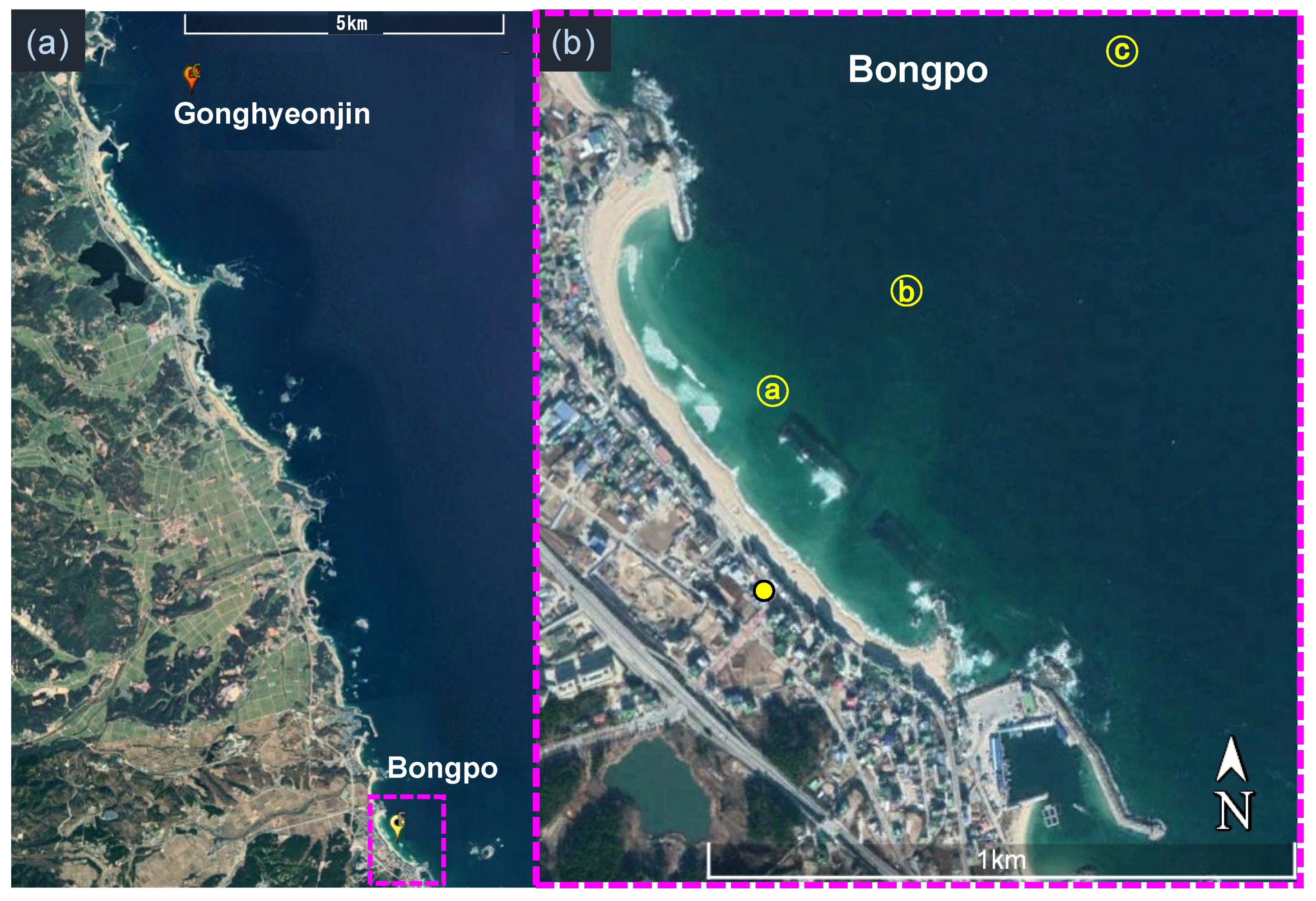
Figure 1a shows the locations of the experimental site, Bongpo Beach, where VMS data were measured and Gonghyeonjin (38°21′40.10″ N and 128°31′41.60″ E) where wave data were measured along the eastern coast of South Korea. The waves were measured by acoustic wave and current (AWAC) meters moored at a depth of 32 m and located ~12 km off Bongpo Beach. The non-directional spectrum for wave height and period was estimated from acoustic surface tracking (AST) spectra of the AWAC, and the three near-surface velocity cells in the AWAC meters calculated the wave directional spectrum. Using Storm, a software program for wave analysis provided by the AWAC meter manufacturer (NORTEK AS), wave parameters such as significant wave height ($H_s$), peak wave period ($T_p$), significant wave period ($T_{1/3}$), peak wave direction (${\theta }_p$), and mean wave direction (${\theta }_{mn}$) were estimated from the AST spectra. The analyzed wave direction is expressed relative to local magnetic north owing to the characteristics of the observation device. In this study, the wave angle was corrected based on grid north by subtracting the grid-magnetic (GM) angle. From 2015 to 2019, wave data were measured continuously without signal loss except for 18 days during April 2016 (11–28 April).

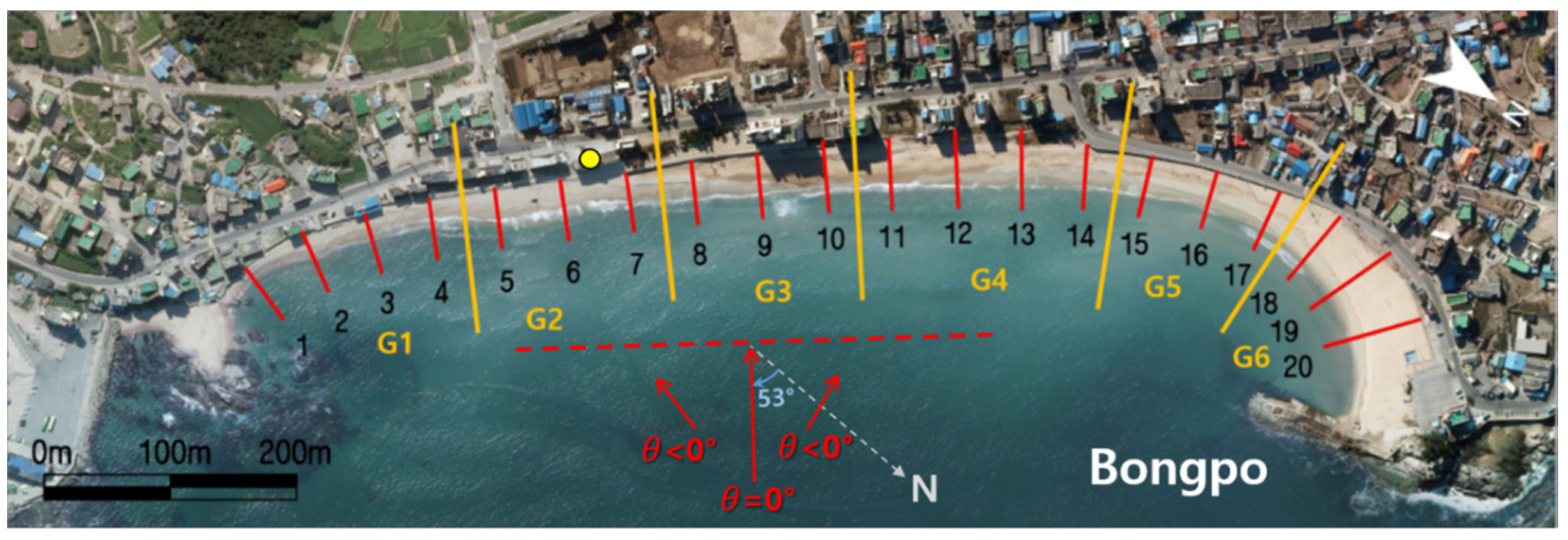
VMS data are available for Bongpo Beach over four years: from June 2015 to July 2019. Bongpo Beach is a pocket beach located on the eastern coast of South Korea (Figure 1). The beach is about 1-km long and faces northeast. The beach mostly consists of sand with a median grain size of 0.46 mm (D₅₀) and a range of over 0.20–0.78 mm. Both ends of the beach are blocked by rocky headlands that contribute to the shape of the pocket beach. Figure 1b shows the map of Bongpo Beach. The VMS was installed at a building marked with a yellow circle on the map, and a total of four video cameras were used by the VMS to monitor the entire beach area. The beachlines at which each beach width was calculated were set along the curved shoreline. In total, 20 beachlines were established at 50-m intervals, starting with #1 at the southern end of the beach.

Coastlines which may be changed rapidly by waves were extracted by averaging 180 snapshot images collected for 3 min, and imaging geometry coordinates were projected onto the ground plane coordinates using reference points set on land. These projected images collected by the four cameras were superposed and synthesized into a planar image of the whole beach. In this image, land and sea were distinguished by the colors of image data pixels. The shoreline position at each beachline was determined by finding locations that satisfied the conditions separating the land from the sea, and beach width was measured from a fixed reference point on the beachline.

Despite the processing of VMS data, the quality and resolution of the estimated beach width data were not sufficiently fine for comparison with wave measurements because of limited visible-light data acquisition capacity at night and in harsh weather. In addition, coastlines can be incorrectly extracted owing to noise or erroneous image detection; therefore, it was necessary to improve the quality of the beach width data. Since the quality of the beach width data varies according to the beachline and the period, and because the outlier pattern appears differently, it was necessary to improve the accuracy of the data by considering the characteristics of each beachline. To achieve this, we smoothed the beach width data by applying a moving median, detecting and eliminating outliers from the smoothed basis for all beachline data. Gaps due to missing data points were filled from extrapolation of the adjacent raw data with smoothed trend. By assuming that the trend of the raw data and noise should be maintained in the gap of the missing data, the smoothed trend—the trend of raw data in which the outliers were removed—was extrapolated into the gap of the missing data so that the trend could be maintained in the gap. In addition, the noise component was added onto the trend inside the gap as it was obtained by generating random numbers with normal distribution.

The beach width, $W{\left(t\right)}_i$, was measured for all beachlines (i = 1, …, N = 20) along the beach. At each beachline, the time variation of the de-meaned beach width, $\mathrm{𝕪}$, was calculated by

$$\mathrm{𝕪}=W{\left(t\right)}_i-{\mu }_{W_i}$$

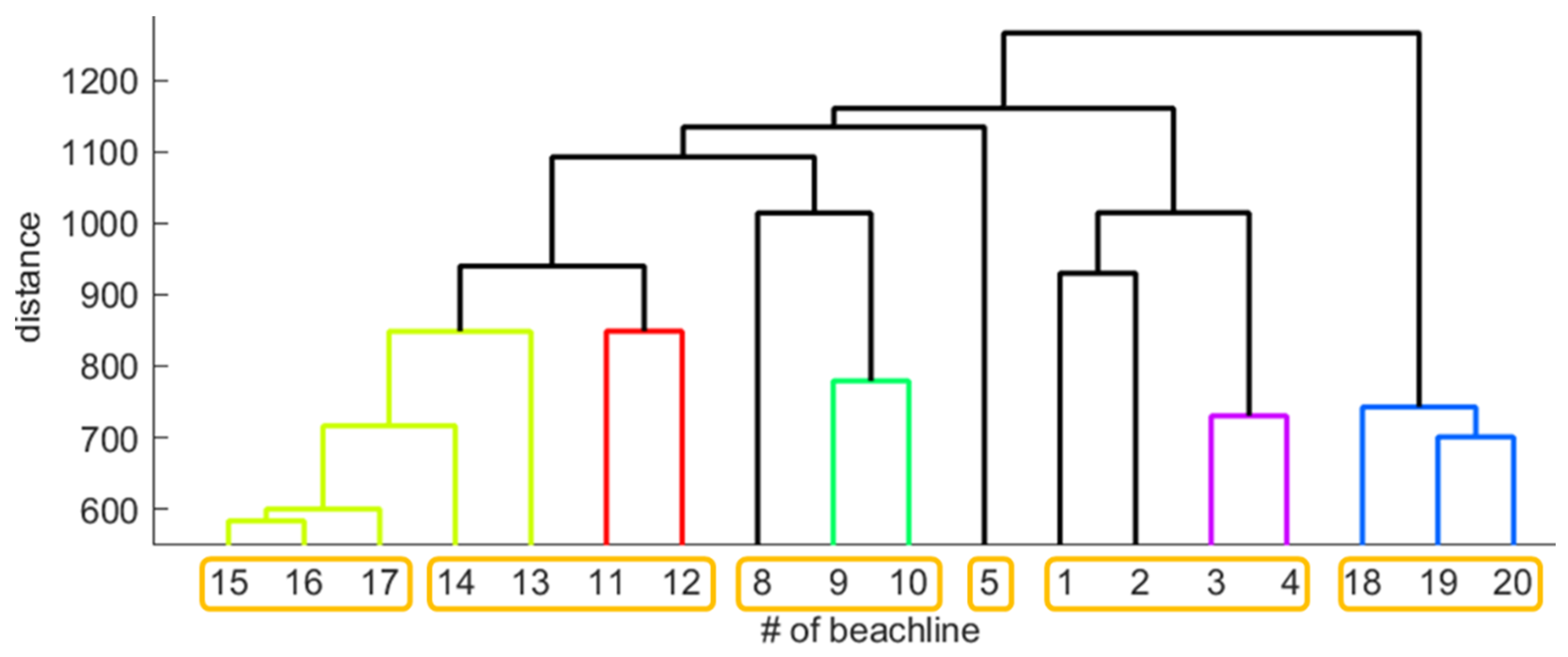
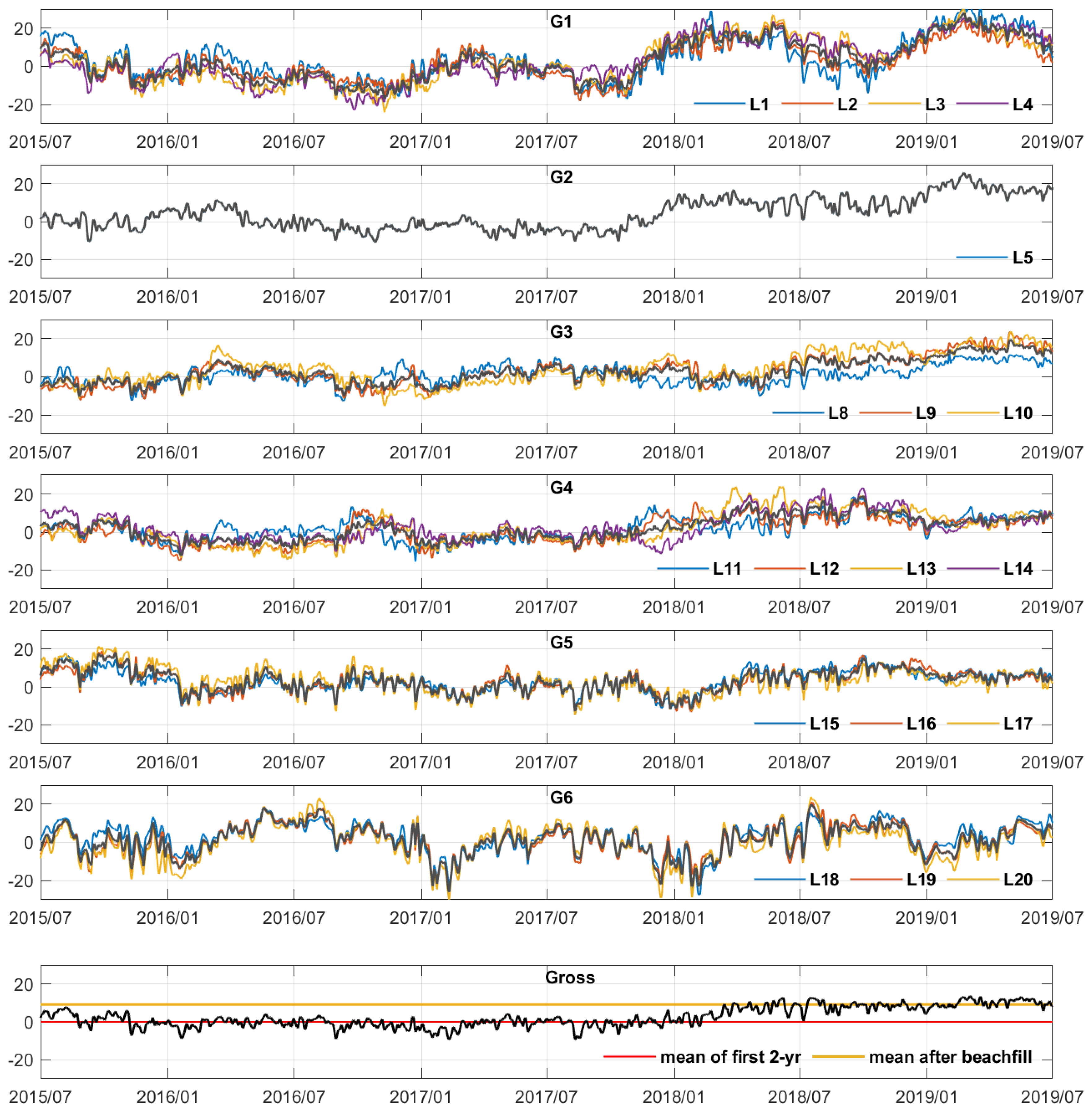
where ${\mu }_{W_i}$ is the mean beach width of each beachline averaged over two years from July 2015 to June 2017. We then divided the beach into six sectors using hierarchical clustering. Figure 2 shows the cluster tree of the beach width data as a result of the clustering. In the figure, the x-axis denotes the number of beachlines and the y-axis denotes the distance between clusters. The grouping of the beachlines was determined by their proximity within the tree. The beach width data were classified into six sectors based on the clustering analysis as shown in Figure 3. Figure 4 shows the time series for $\mathrm{𝕪}$ along the beachlines for each sector; the beach width variation patterns are similar for beachlines that belong to the same sector. In contrast, the different patterns are easily distinguished for different sectors. There is a clear difference between two particular sectors, G3 and G4, even though they are closely located. Therefore, it was necessary to divide these sectors in order to compare the shoreline change patterns between sectors. Variations in beach width were examined by beachline and by sector to understand the trends of sediment movement for each sector. Unfortunately, the data on beachlines 6 and 7 were not available due to low quality of VMS images. The trend of beach width change on beachline 5 is distinguished from those in G1 and G3; however, we separated the data of beachline 5 into G2 so that the data were grouped into a total of six sectors. Although G2 was distinguished from other sectors, its data were compared two times in the manuscript by combing with G1 or G3–G5 because its data showed similar pattern with G1 at some points but similar with G3–G6 at other times. We did not compare the G2 data alone as it is less significant.

The time series of gross beach width (summation of all sectors) is plotted in Figure 4g over the four years of the experimental period. It clearly shows that the range of variation is much smaller compared to those for individual sectors shown in Figure 4a–f. This indicates that the total sediment budget might be conserved within the pocket beach. The red line in Figure 4g marks the level of mean beach width that was averaged over the first 2-year data before the beach was filled in 2018. It shows that the beach width was fluctuated from the mean level in month-scale. However, there was no clear trend of increasing or decreasing of $\mathrm{𝕪}$ during the 2-year period, indicating no loss and gain in the total sediment budget occurred in this pocket beach. In addition, the standard deviation of $\mathrm{𝕪}$ variation was 3.3 m with maximum and minimum values of 7.7 and −9.3 m, respectively, which were smaller than those for individual sectors. This pattern of beach width conservation for all sectors is also observed after the beachfill. In 2018, when the beach was nourished, the total $\mathrm{𝕪}$ gradually increased. Once the beachfill was completed, however, the beach width remained unchanged though it was highly fluctuated. The yellow line in Figure 4g marks the level of averaged $\mathrm{𝕪}$ over the last 1-year period after the beach fill. It also shows that no increasing/decreasing trends were observed in gross beach width with the mean level of 9.2 m. The standard deviation was 2.1 m with maximum and minimum values of 13.5 and 3.1 m, respectively.

2.2. Longshore Sediment Transport

Under severe wave conditions such as storms, sand particles move offshore vigorously and change the beach profile. Before long, however, the beach profile returns to its pre-storm condition as the eroded beach profile is slowly recovered owing to onshore sediment movement under milder wave conditions. The cross-shore sediment transport rate, $Q_y$, is influenced by the severity of the wave condition, but the beach change caused by the successive cross-shore sediment transports appears as a seasonal change [15]. Meanwhile, the longshore currents induced by obliquely incident waves produce longshore sediment transport that carries sediments along the shore. This may cause shoreline variations that usually last longer than the changes made by cross-shore sediment transport. On this basis, it is assumed that shoreline changes depend mainly on longshore transport, $Q_x$, which can be simplified according to one-line theory [25].

From sediment continuity in one-line theory, the displacement of the shoreline per unit time and the volume change (longshore sediment transport rate, $Q_x$) are related by Equation (1),

$$\frac{\partial y}{\partial t}=-\frac{1}{h}\frac{\partial Q_x}{\partial x}$$

(1)

where the displacement of the shoreline, y, is equivalent to the beach width change, and h is the profile depth, which is equal to the closure depth plus the beach berm height.

Thus, the longshore sediment transport rate is proportional to the magnitude of the profile depth and the time derivative of the shoreline change:

$$Q_x=-h\int \frac{\partial y}{\partial t}dx$$

(2)

The beach profile is regarded as invariant for a long-term period [15]. Moreover, shoreline changes fluctuate more than profile depth changes, and so we assumed that $h$ was constant in this study. Therefore, for long-term variation, the (proportional) magnitude of the longshore sediment transport rate can be estimated by the proportional time derivative of the shoreline change without knowing the profile depth:

$$Q_x\propto \int \frac{\partial y}{\partial t}dx\approx \frac{\partial }{\partial t}\int ydx$$

(3)

2.3. Wave Energy and Storm Intensity

The principal wave parameters that affect the beach width are wave height, wave period, and wave direction; the wave energy calculated from these parameters may also be important. The energy flux, which is the average energy per unit of time in the wave propagation direction, is derived based on linear wave theory. The following wave power per unit width can then be obtained:

$$P=\frac{{\rho }_{w}g{H}^{2}L}{16T}\left(1+\frac{2kh}{\sin 2kh}\right)$$

(4)

where ${\rho }_w$ is the density of seawater (1025 kg/m³), $g$ is the gravitational acceleration; $h$ is the water depth; and $H,L,T,k\left(=2\pi /L\right)$ are the wave height, length, period, and wave number, respectively.

Equation (4) expresses the wave force but can be applied only to regular waves under the assumption of linear waves; however, real ocean waves are represented by the superposition of numerous waves with different heights and periods. The wave power based on the spectrum of realistic irregular waves can be expressed by averaging the power of individual regular waves as follows:

$$P=\frac{{\rho }_w{g}^2}{64\pi }{H}_s^2{T}_z$$

(5)

where $H_s$ is the significant wave height and $T_z$ is the zero up-crossing period. The longshore component of the wave power along the coast can be obtained as

$$P_y=P\cos \theta \sin \theta$$

(6)

where $\theta$ is the direction of the incident waves at the shore face. The shore normal direction is set as 0° and the directions of waves propagating left and right of the normal direction are set as (−)° and (+)°, respectively.

Thus, the $P_y$ of incoming waves can have a positive or negative values depending on their propagation direction, and the maximized magnitude of wave power can be obtained when waves approach the shore at ±45° from the shore normal direction. At the experimental site, Bongpo Beach, the shore normal direction is at 53° N. Therefore, the wave power acting from north to south increases when $P_y$ is negative and its magnitude is maximized with an incident wave angle of 8° N. Similarly, the power from south to north increases when $P_y$ is positive and is maximized at 8° S.

The duration of high waves, such as during storms, is also an important factor in beach width change. The definition of a storm event, with representative high waves, is site-specific (cf. [18,27]). In general, $H_{95\%}$ and $H_{99\%}$ are used as thresholds for storm determination, and the time between two storm events is included in the storm period if it is within the given criterion. According to Masselink et al. [28], a storm is defined as a wave event during which the maximum $H_s$ exceeds the 1% exceedance wave height ($H_{99\%}$), where the start and end of the storm event occur when $H_s$ exceeds or falls below the 5% exceedance wave height ($H_{95\%}$), respectively. Following the approach proposed by Dolan and Davis [29], a storm event is defined when $H_s$ exceeded $H_{95\%}$ during a complete tidal cycle, meaning over a period of 12 h. A succession of two or more storms, where the calm period between events is less than five days, is then considered as a cluster of storms.

In the present study, $H_{90\%}$, $H_{95\%}$, and $H_{99\%}$ were employed as thresholds for significant wave heights to define storm events for analysis of beach width variation. Based on this, we classified storm events into three levels—Level 1 (S90), Level 2 (S95), and Level 3 (S99)—with a periods of significant wave height above the 90th, 95th, and 99th percentile wave heights, respectively. High wave events with periods of less than one hour were disregarded, and the time between two events less than 5 hours apart was included as the duration for a single storm event.

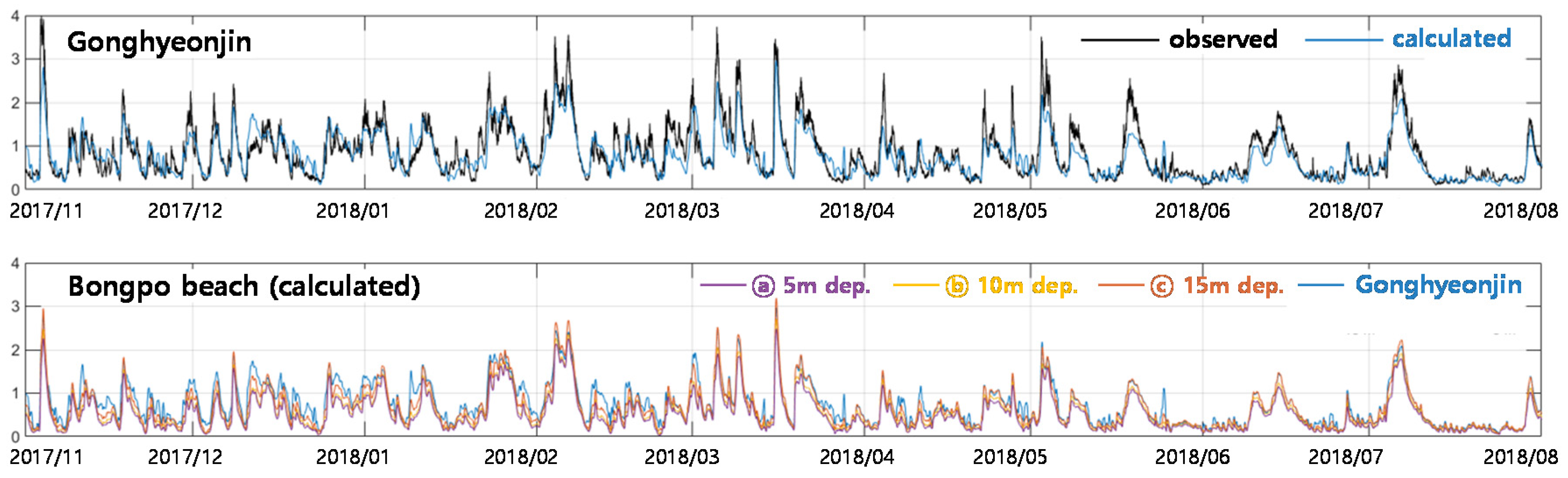
It should be noted that the wave conditions in the experimental site, Bongpo Beach, were used as they were observed in Gonghyeonjin Station that is located ~12 km away from the beach as shown in Figure 1a. The validation was performed through SWAN wave model. The results showed that the model nicely simulated the observed data with high correlation coefficient (0.88 for wave height and 0.79 for wave period). In Figure 5a, the time series of the observed and modeled wave heights are compared at Gonghyeonjin Station, which shows that the model nicely simulated the observed data. In addition, the model data calculated at 5-, 10-, and 15-m water depths of the Bongpo Beach (these depths are marked in Figure 1b) are also similar to the observation data at Gonghyeonjin Station, showing good agreement between model and measured wave heights at the three water depths (Figure 5b). The good agreements between the observation and model data were found in wave period and propagation direction as well. For the wave propagation direction, however, the wave direction in G5 and G6 could be significantly different due to the orientation of the coastline. The impact of coastline orientation was tested in the initial stage of the analysis, but the results were not distinguished from those without considering the coastline orientation, likely due to the short beach length (~1 km). Therefore, we assumed that the wave conditions were similar between the two locations and thus applied the observation data for the wave conditions in the experimental site.

3. Results

3.1. Long-Term Shoreline Response

The daily variation of beach width $y$ for all beachlines are contoured over four years from June 2015 to July 2019 in Figure 6a, where the numbers along the y-axis represent the beachlines as marked in Figure 3. Figure 6a shows that the beach width actively varied not only in time but also in space along the coastline, although the variation pattern is not so regular. From January 2018, $y$ in the G1 and G2 areas rapidly increased owing to beach nourishment (23,500 m³). Therefore, the patterns in $y$ after nourishment should be distinguished from those before it.

For the southern part of the beach (beachlines 1–5), $y$ rapidly decreased (i.e., the beach was eroded) from November 2015 and this continued until February 2017. Erosion also occurred along the mid-part of the beach (beachlines 10–15) starting from January 2016. In the northern part of the beach (beachlines higher than 15), $y$ increased from March 2016, indicating that the sediments eroded from the middle region moved to the north during this period. These changes in beach width resulted from seasonal fluctuation of total sediment transport due to effective wave action.

To separate the influence of longshore transportation from overall change implying seasonal recurrence, we differentiated $y$ with respect to $x$ and $t$. Figure 6b,c display the distributions of $\partial y/\partial x$ and $\partial y/\partial t$, respectively. To remove noise caused by daily variation and obtain longer-period changes, $y$ for each beachline was averaged (monthly) before differentiation.

The pattern of $\partial y/\partial x$ in Figure 6b confirms longshore sediment movement. For example, large values of $\partial y/\partial x$ gradually moved from beachline 10 in September 2016 to beachline 15 in February 2017, which shows that sediment moved to the north from the middle of the beach during this period.

It should be noted that the pattern of $\partial y/\partial t$ in Figure 6c shows clearer seasonal repetition, specifically in winter, regardless of nourishment. For example, $\partial y/\partial t$ increased in the southern part of the beach (beachlines 1–10) in January of each year from 2016 to 2019, while it decreased in the northern part (beachlines 11–20) during almost the same winter period each year. This indicates that sediments at this beach might be transported from north to south along the coast during winter.

Figure 6d shows integrated beach widths along the coast; $\int ydx$ are plotted to show the trend of gross variation of beach width. Although the patterns in sectors G1 and G6 are slightly different, the total beach area gradually decreased until the end of 2017 but rapidly increased early in 2018 after beach nourishment. Compared with total beach width, $\partial y/\partial x$ and $\partial y/\partial t$ in Figure 7b,c do not include the beach fill effect and thus show time variation patterns of shoreline changes more clearly.

The integral of the rate $\partial y/\partial t$ along the coast, $\int \partial y/\partial tdx$, is also presented in Figure 6e. This quantity is related to the time variation of LST, $Q_x$, as described by one-line theory in Equation (2). It should be noted that there are times when $Q_x$ values changed significantly within a period of several days. These periods of rapid change in $Q_x$ are likely related to periods of storm wave attacks, especially S99, which lasted more than 24 h (hereafter S99_24hr+). In Figure 6, periods under the effect of S99_24hr+ are indicated by vertical gray lines in all panels. In addition, each storm event for S99_24hr+ is marked in Figure 6e by a circle with a diameter representing the storm intensity. The storm intensity was calculated as the product of (maximum significant wave height during the storm event)² and the storm duration. The color of the circle represents the most frequent wave direction during each storm event with respect to the color bar on the left side.

After every storm event when S99 lasted more than 24 h, $Q_x$ increased significantly. Thus, it can be seen that severe wave conditions above a certain threshold can cause changes to the shoreline by increasing $Q_x$; this change can last for months. This result indicates that LST caused by S99_24hr+ events resulted in conspicuous shoreline changes that lasted longer than changes made by cross-shore sediment transport. In the absence of S99 lasting more than 24 h, $Q_x$ decreased before beach nourishment in early 2018. In Figure 6f, $Q_x$ is estimated for the south (G1), middle (G4), and north (G6) parts of the beach. After every S99 event, a positive peak in $Q_x$ was observed in G1 first, with peaks in G4 and G6 occurring later in the sequence. This indicates that sediments were transported to the north along the beach after severe wave events regardless of nourishment. Especially in January 2017, when the storm power intensity had sharp peaks, $Q_x$ in the G1 sector subsequently increased. Afterward, gross $Q_x$ and sectoral $Q_x$ in sectors G4 and G6 also increased. This indicates that sediment transport actively occurred in sector G1 and that sediments moved first to G4 and then toward G6.

In addition, weekly and monthly cumulative wave powers $P$ are displayed in Figure 6g. The cumulative $P$ gives supplemental information on the behavior of LST. Especially in 2018, after beach nourishment, LST significantly increased, although the wave conditions were not severe even in the winter season. In addition, LST had a sharp peak in January 2019 after a slight increase in cumulative $P$ (Figure 6e). It is likely that sediment transport was accelerated even by small wave actions when the beach was filled with excessive sand after nourishment.

3.2. Short-Term Change in the Winter Season

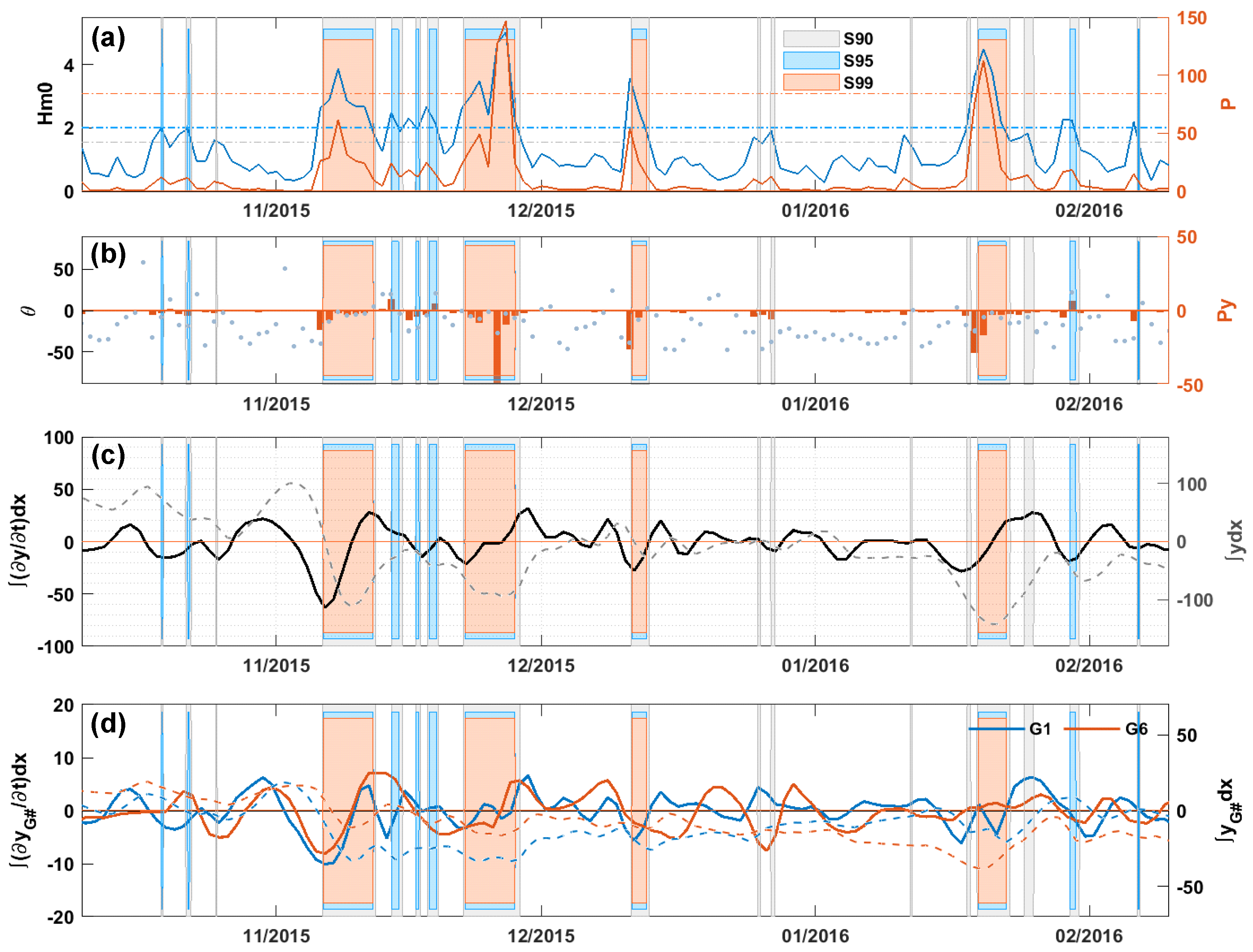
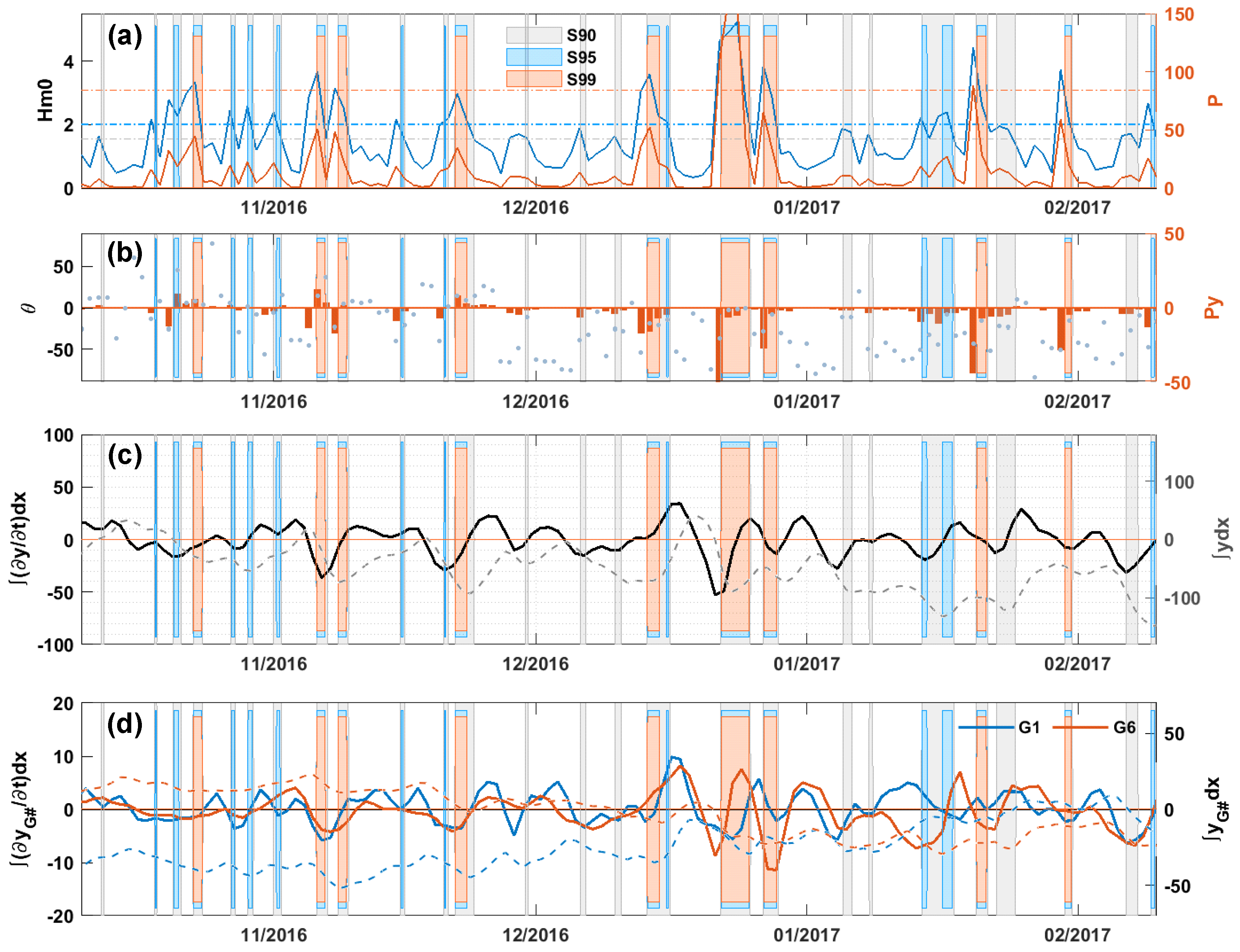
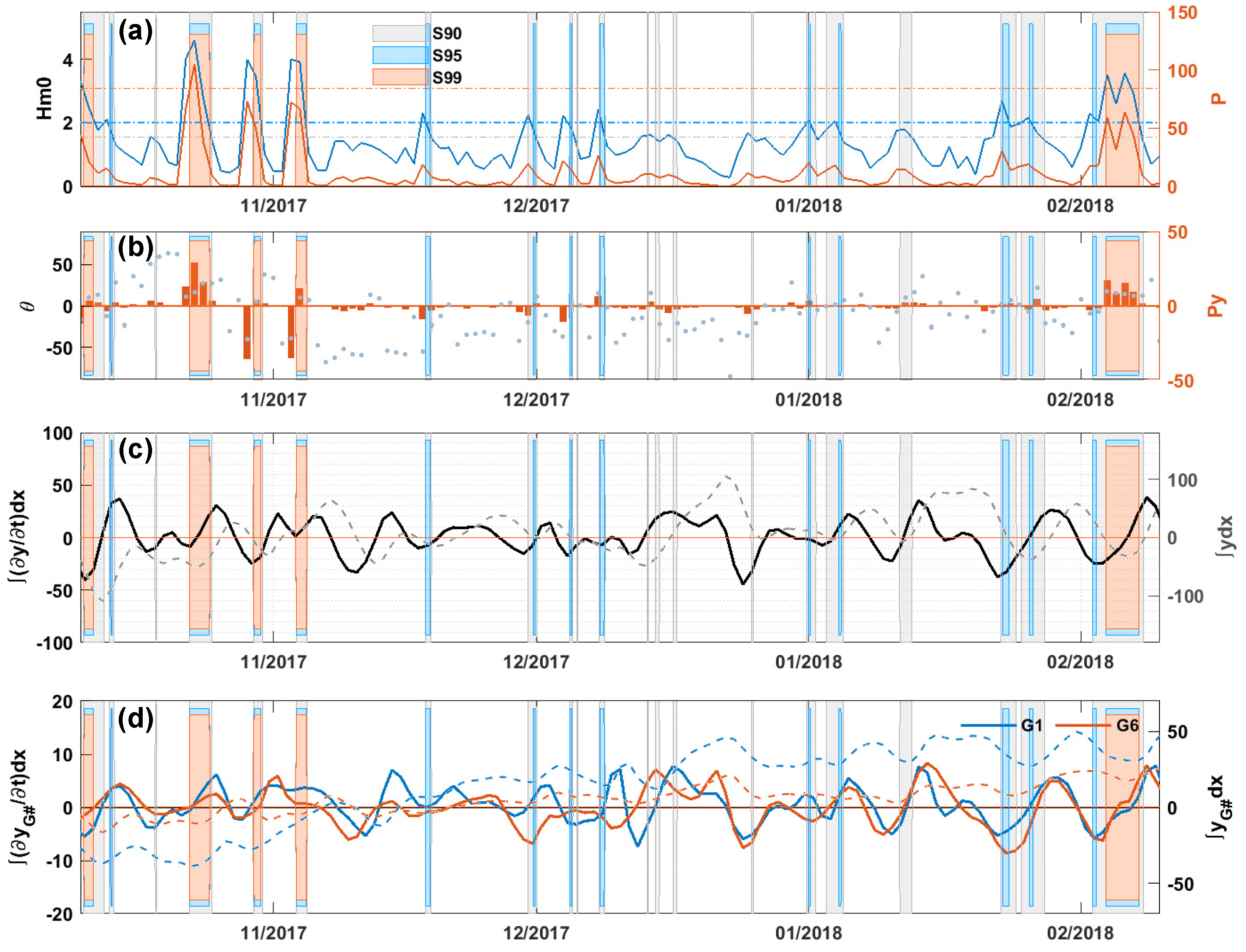
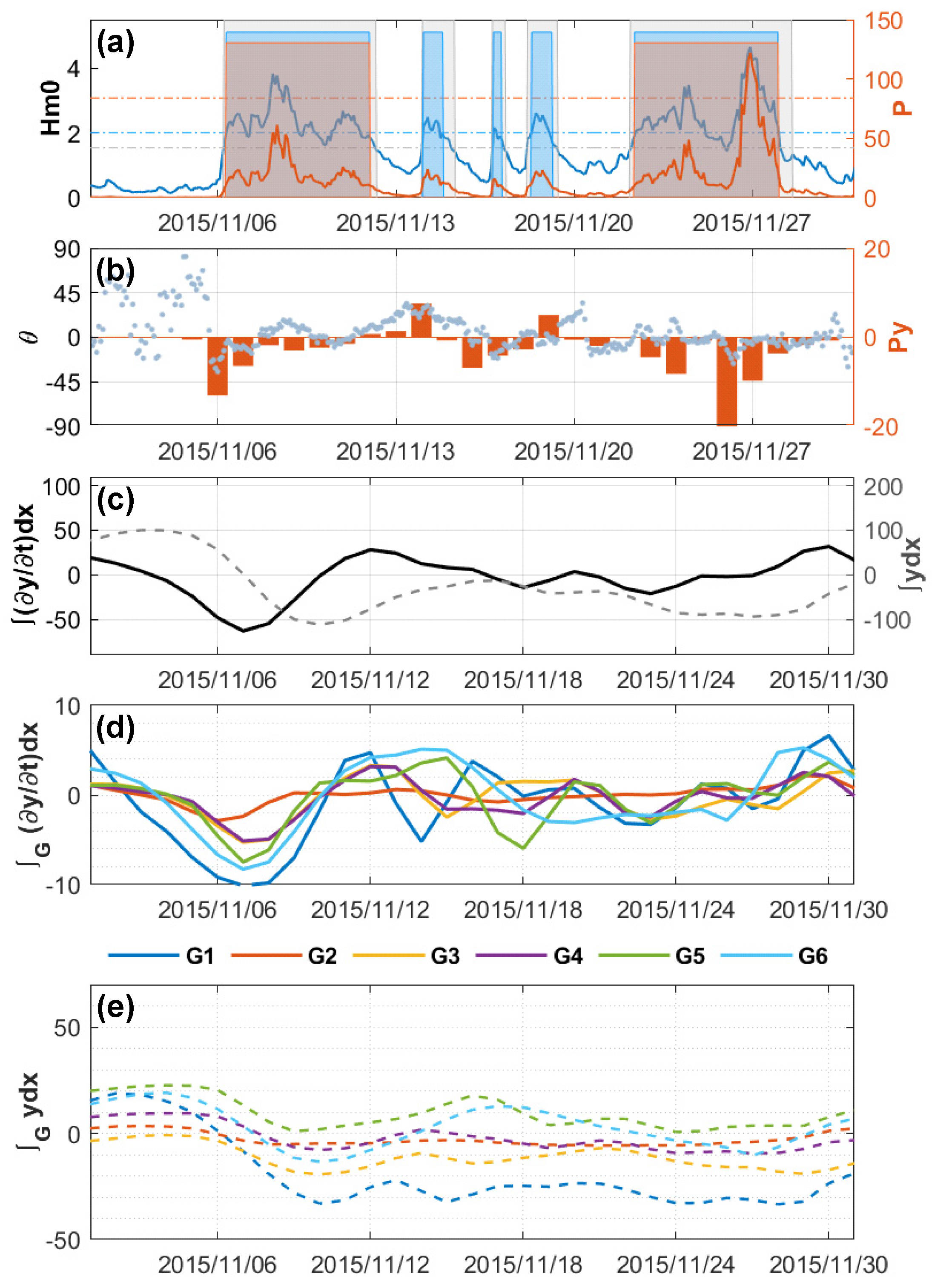
Figure 7, Figure 8, Figure 9 and Figure 10 show the time variation of wave parameters $Q_x$ estimated by Eqation (3) and beach width during four winter periods between 2015 and 2019, respectively, with an indication of high-wave-event periods. The first panel shows the daily mean of significant wave height $H_{m0}$ along with the daily mean of wave power $P$. The second panel shows the daily mode of $P_y$ along with the daily mode of wave direction ($\theta$). Negative or positive values in the second panel imply that the waves propagate from the left or right side of the shore, respectively. In the third panel, the daily integrated beach width along the coast $\int ydx$ is plotted with a dashed line to show the trend of gross variation of the daily beach width along with $\int \partial y/\partial tdx$, as it is related to $Q_x$ (solid line). Since it is an integration of the beach width for all beachlines, $\int ydx$ is equivalent to the ‘gross beach width’. Similarly, ‘sectoral beach width’ can be defined as the integration of beach width, $y$, for the beachlines in each sector as ${\int }_{\mathrm{G}\#}ydx$. In the last panel, $\int ydx$ (dashed line) and $\int \partial y/\partial tdx$ (solid line) in sectors G1 and G6 are presented separately. Here, the zero line indicates the average over the observation period and thus the positive and negative values of $\int ydx$ and $\int \partial y/\partial tdx$ indicate higher or lower values over the average, respectively. In every panel, columns in gray, blue, and red represent storm periods of S90, S95, and S99, respectively. Since periods over $H_{99\%}$ also qualify as periods over $H_{95\%}$ and $H_{90\%}$, the columns of S99 include the columns of S95 and S90. Similarly, the columns of S95 include those of S90.

The change of beach width represented by $\int ydx$ and $\int \partial y/\partial tdx$ during high-wave events is more conspicuous than that during periods of lower waves. During the winter between 2015 and 2016, as shown in Figure 7, a total of four S99 events were observed. The first two S99 events were characterized not only by the wave intensity but also by their duration, as they lasted longer than five days. The third and fourth S99 events lasted for two and three days, respectively. In all S99 events, the total beach width $\int ydx$ decreased considerably (dashed line in Figure 7c), which indicates that the beach was rapidly eroded owing to offshore movement of beach sediments by the storm waves, as has been commonly observed (e.g., [30]). It should be noted that, following the decrease in $\int ydx$, the estimated LST, $\int \partial y/\partial tdx$, increased; then, the eroded beach width began to recover as the decrease in $\int ydx$, the increase of $\int \partial y/\partial tdx$, and the recovery of $\int ydx$ occurred sequentially for S99 events. The recovery of beach width after strong LST was likely related to $P_y$ (Figure 7b) rather than $P$ (Figure 7a), confirming the role of wave direction. As shown in Figure 7d, during the winter after the two S99 events, ${\int }_{\mathrm{G}1}ydx$ increased while ${\int }_{\mathrm{G}6}ydx$ decreased owing to the negative wave direction. This indicates that the sediments were eroded from sector G6 and transferred to sector G1 by strong LST. It also shows that the beach width gradually recovered after severe erosions while the sediments were generally moved alongshore, not offshore, by the obliquely incident waves. The beach width eroded by the first S99 event in November did not recover its pre-storm condition during the rest of the winter period. It is likely that the first attack of strong S99 that lasted more than five days resulted in a non-recovery condition. Moreover, the time gap between the first and second S99 events was relatively short (only 10 days), which prevented the beach from recovering. In addition, three short S95 storms developed between the first and second S99 events, which also reduced the beach’s resilience for recovery.

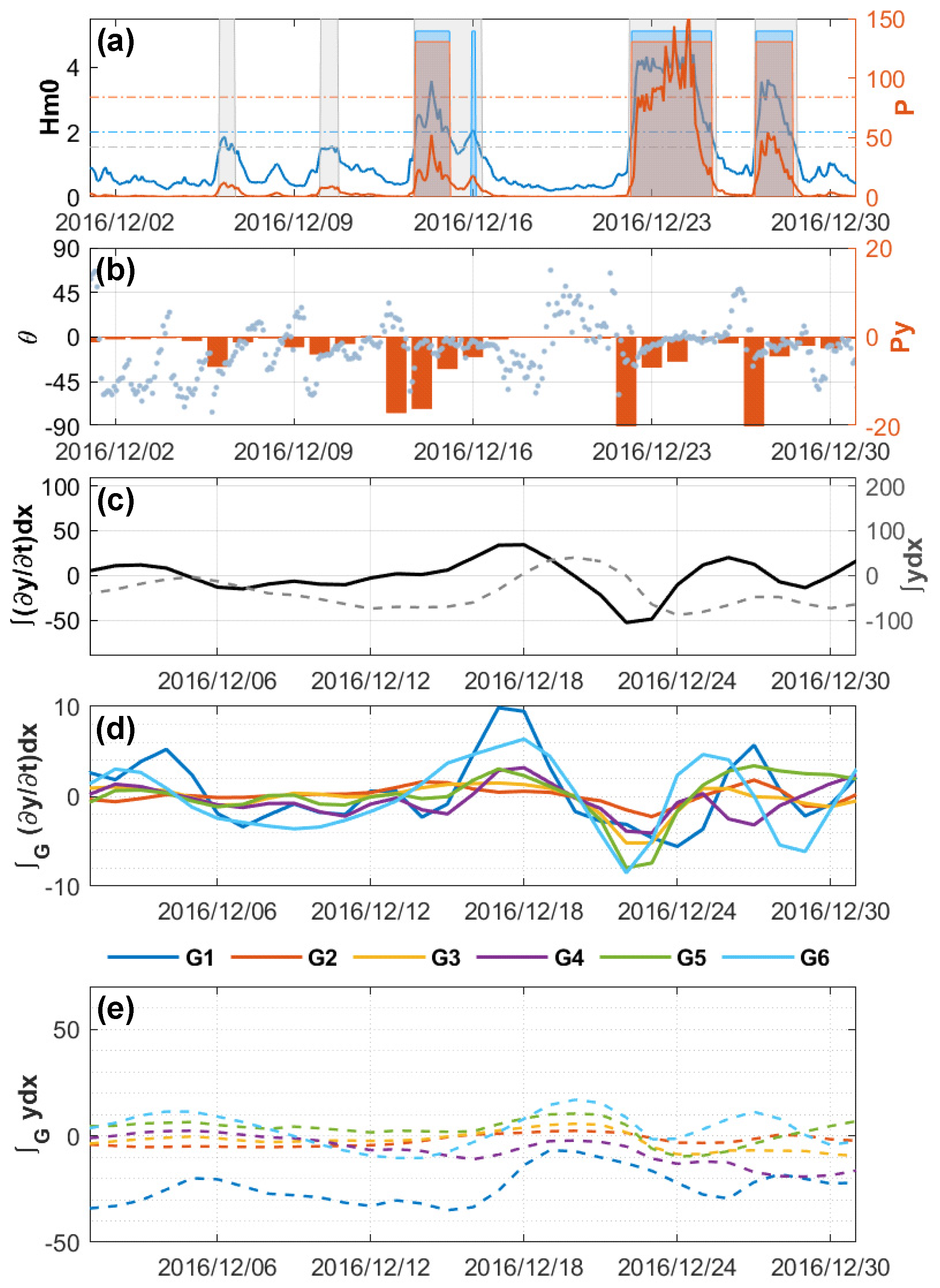
In the winter between 2016 and 2017 (Figure 8), there were more frequent storm events but with lower intensity and shorter duration than during the previous winter season. Owing to frequent storm attacks, the total beach width gradually decreased as the magnitude of $\int ydx$ became lower at the end of the winter compared with that at the beginning (dashed line in Figure 8c). This indicates loss of sediments by dominant offshore sediment transport under harsh wave conditions over the winter period. In addition, $\int ydx$ variation patterns at the two end sectors of G1 and G6 showed clear differences for this winter; $\int ydx$ in sector G1 increased, whereas $\int ydx$ in sector G6 decreased (dashed lines in Figure 8d). This shows that sediments were moved from sector G6 to sector G1 by LST. The opposite trend by sector confirmed the role of LST caused by the action of obliquely incident waves in the winter season, as in the previous winter. Figure 8c also shows that $\int ydx$ increased following the increase in $\int \partial y/\partial tdx$ during storm events, confirming that the beach width increased as LST increased, as observed in the previous year. Therefore, although the gross beach width generally decreased owing to stronger offshore sediment transport, there were times when the beach recovered according to the increase in LST.

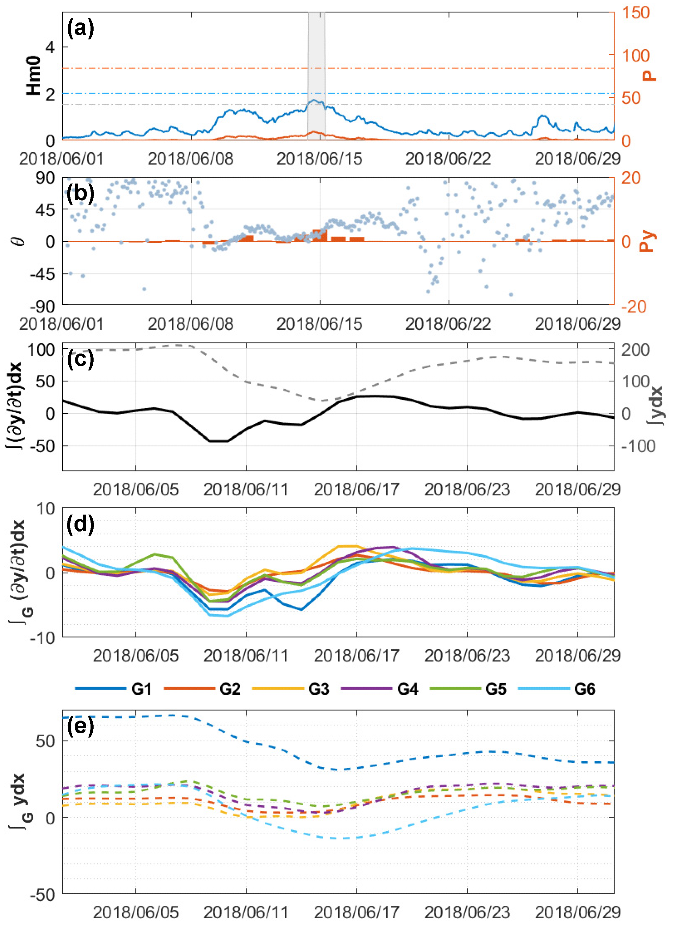
This specific pattern was also observed in the winter between 2017 and 2018 (Figure 9), when the beach width increased following the increase of LST during severe storms. However, in general, the beach width increased as $\int ydx$ at the beginning of the season was lower than that at the end. This increment of beach width can also be seen clearly in Figure 9d, where $\int ydx$ gradually increased over the winter period for both G1 and G6, indicating that LST during storm events did not contribute to overall shoreline variation. This likely reflects a long low-wave energy period between December 2017 and February 2018, during which no S99 events were observed. Therefore, the shoreline erosion by storm waves at the beginning of the winter was recovered during the time of weaker wave conditions, when obliquely incident waves were dominant.

In the winter between 2018 and 2019 (Figure 10), the wave conditions were milder compared with those of previous winters. There were no S99 storm events observed and even the number of S90 and S95 were also significantly smaller compared with previous winter seasons. In addition, the level of $\int ydx$ was significantly higher compared with that in previous seasons. This high $\int ydx$ was due to beach nourishment implemented in early 2018, which provided a significant amount of sediment. The magnitude of wave energy was lower, but the beach width was significantly higher than during other winter seasons (see different scale on the y-axis of Figure 10 compared with those of Figure 7, Figure 8 and Figure 9). Despite having the mildest wave conditions, the variation pattern (where LST increments follow beach width reduction owing to CST during storm events) was repeated in this season. Following increments in LST, the eroded beach width gradually began to recover. Moreover, clearly different patterns between $\int ydx$ in two sectors were also detected. The increased and decreased beach widths in sectors G1 and G6 resulted from obliquely incident waves during this winter season.

3.3. Event-Scale Analysis

We investigated the patterns of observed shoreline variation in terms of wave conditions during specific events including both severe and rapid variations in cases of extreme storm conditions, and the shoreline response under milder wave conditions.

When extreme storm conditions (S99) lasted more than five days, the beach was rapidly eroded by CST. For example, Figure 11 shows that, when storm waves attacked the beach on 6 November 2015, $\int ydx$ (dashed line) rapidly decreased, indicating erosion. However, the LST estimated by $\int \partial y/\partial tdx$ (solid line) did not start to increase until 7 November 2015, although $P_y$ peaked on 6 November 2015. This indicates that the beach was first eroded owing to CST but LST responded later to obliquely incident waves. A similar pattern occurred on 22 November 2015, when another S99 storm event started. While $\int ydx$ decreased, corresponding to a storm event, LST only started to increase on 23 November 2015, one day after the storm beginning (22 November 2015). The combined effect of CST and LST during extreme storm periods resulted in a characteristic recovery pattern following the storm. In general, the shoreline eroded by CST was recovered in most sectors of the beach. However, in some sectors the shoreline recovery was slower; this occurred when sediment was lost by LST. For example, $\int ydx$ in most sectors gradually increased owing to recovery; however, the recovery was not clearly observed in sector G1 as the sediments in this end sector were likely lost by LST. Figure 12 (December 2016) shows a similar pattern; $\int ydx$ decreased when an S99 event occurred and $\int \partial y/\partial tdx$ increased following erosion. Specifically, the beach width in sector G1 sharply increased after 16 December 2016 following the end of an S99 event, while $\int ydx$ at other sectors did not show clear changes. This indicates that sediments moved to sector G1 owing to LST caused by the storm events.

Under milder wave conditions, rapid and significant changes in beach width did not occur. Instead, LST caused by obliquely incident waves carried sediments along the beach toward the end sectors. In Figure 13, neither $\int ydx$ or $\int \partial y/\partial tdx$ show significant changes from 15 November until 7 December 2017. However, the beach width in sector G1 gradually increased, while it decreased in sectors G5 and G6. In the corresponding period, $H_{mo}$ remained less than 2 m but the wave propagating direction, $\theta$, actively varied from 0 to +90°, indicating that waves were approaching from the left of the beach (Figure 3). Therefore, sediments were consistently moved alongshore toward sector G1 by LST, regardless of low-wave energy corresponding to negative values of $P_y$.

3.4. Shoreline Response after Beach Nourishment

One of the most significant changes in beach width during the experimental period was caused by beach nourishment implemented in early 2018. As shown in Figure 6a, the beach width sharply increased in sectors G1–G4 from January 2018, showing that nourished sediments were placed in sectors near the southern end of the beach. As a result, after the nourishment, the total beach width, $\int ydx$, increased from about 30 m² in early 2018 to about 150 m² in early 2019 (Figure 6d). When a large amount of sediment was placed on the beach face by nourishment, the shoreline rapidly responded to reach equilibrium in both cross-shore and longshore directions. In Figure 14, the wave and shoreline parameters are plotted for a period of about one month in June 2018, when the nourishment had been completed. Starting from 8 June 2018, $H_{mo}$ and the magnitude of $P_y$ increased for about 10 days until 18 June 2018. However, the increment of wave power was not significant compared with those observed in storm periods such as S90–S99, and even the maximum wave height was less than 2 m. However, the total beach width, $\int ydx$, rapidly decreased from June 8 to 16 June 2018, and the LST estimated from $\int \partial y/\partial tdx$ increased over the same period (Figure 14c). The significant changes in the beach width and LST regardless of the comparably low wave energy in this short period likely occurred because the beach reached its equilibrium status after nourishment. For example, the beach width in sector G1 sharply decreased while $\int ydx$ in sectors G2–G5 did not change significantly. Considering that the nourishing sediments were placed at the southern end of the beach, the rapid change in sector G1 can be explained by the equilibrium process.

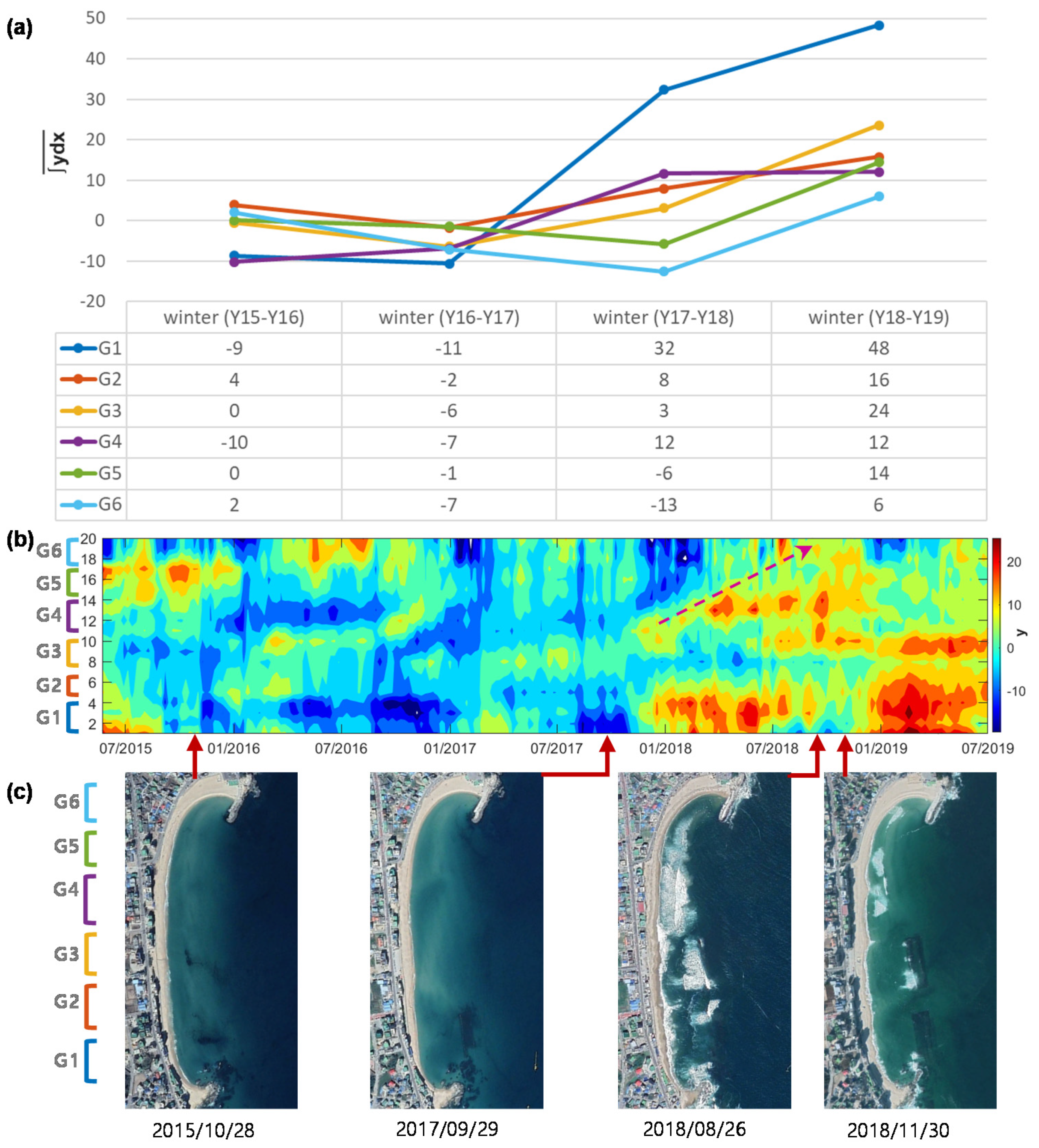
In Figure 15a, the gross beach width is compared between sectors for each winter from 2015. It is clearly seen that the beach width in sector G1 immediately increased immediately after nourishment in the winter between 2017 and 2018. After that, beach width increased with increasing sector number, as the increment of beach width in sector G6 was at a minimum in the winter between 2018 and 2019. This pattern is also observed in Figure 15b where the beach width distribution in all sectors is contoured. The red dashed arrow in the figure shows that the sediments that were placed in the lower sectors gradually moved to higher sectors as soon as nourishment was implemented, which can be observed in the aerial photographs taken from Google Earth at four different times steps during the observation period (Figure 15c).

The impact of the beach fill in which sediments were placed at lower sectors only in early 2018 was not immediately reflected in higher sectors such as G5 and G6. Therefore, beach widths in sectors G5 or G6 still displayed an erosional trend in the winter of 2017–2018, which continued from the previous winters. Before the beach fill of early 2018, all sectors showed the same decreasing trend until the winter of 2016–2017. Therefore, if there was no beach fill, the erosion trend would have continued in all beach sectors, although the rate of erosion might have diminished as waves became milder in subsequent winters.

4. Discussion

One of the most significant findings of this study was that gross beach width started to recover in the late phases of severe storms. When storms occurred, the beach underwent severe erosion as reported in many other studies [19,20]. However, before a storm ended, the beach width started to increase rapidly, reaching close to its previous state after several days. Previous studies have reported rapid recovery after storms, and pointed out that the degree of recovery and time required for it are site specific [31,32]. In this study, such beach responses were clearly observed during the winter season between 2015 and 2016, when the most severe, long duration storms occurred (Figure 7). Furthermore, similar processes repeatedly occurred during other winter seasons when severe storms attacked, although they were less conspicuous (Figure 8, Figure 9 and Figure 10). Interestingly, the estimated LST started to increase several days before the beach width increased. The reason for this specific beach evolution pattern is not yet clearly understood based on the data sets available in this study. However, considering the obliqueness of incident waves during the storms and that the experimental site is a pocket beach where total sediment budget is expected to be conserved, it is likely that strong offshore sediment transport was weakened when LST carried sediments alongshore and deposited them in the corners of the pocket beach. This has resulted in a temporary increase in gross beach width because the sediments were not lost by LST within the pocket beach.

LST was estimated by applying one-line theory, and the time variation of beach width along the 20 baselines could be converted to estimates of LST. One-line theory, which has usually been applied in straight beaches does not consider the details of hydrodynamics and sediment dynamics in the nearshore region of a pocketed beach. Although this application of the theory might induce errors, the long-term pattern of beach width variation agreed reasonably well with the estimated LST pattern based on measured wave conditions. The application of one-line theory to this pocket beach might have been successful owing to the uniform alongshore variation of the beach. In many pocket beaches along the eastern coast of Korea, crescentic nearshore sandbars have developed, creating specific beach evolution patterns caused by the feedback between sandbars and the shore. These patterns cannot be explained by one-line theory. For example, Chang et al. [26] observed locations along the shore of a pocket beach where erosion and accretion rates were larger compared with other areas, corresponding to the development of crescentic sandbars. In the beach considered in this study, locality in shoreline evolution due to sandbars was not observed.

Although the data obtained from the VMS in this study present meaningful results in which LST was estimated based on one-line theory, this application remains limited. For example, the observed relationship between wave measurement and shoreline response was not validated with analyses in detail, and the hydrodynamics in the surf zone that play important role in coastal processes were not considered to estimate LST. The longshore current results from the oblique breaking of waves owing to the reduction of radiation stress by dissipation. The consequent LST should be also related to the wave breaking, and the majority of LST formula are in fact based on wave parameters at breaking point of the surf zone (e.g., [33]). In the present study, however, the results were analyzed based on deep water wave conditions though the LST rate in Equation (1) results from breaking waves, which might result in erroneous interpretations.

In addition, the one-line theory is based on the assumption that the shoreline changed as a result of alongshore sediment budget changes caused by wave energy and direction only, and thus the impacts of seabed topography on nearshore hydrodynamics cannot be considered. These issues have not been considered or resolved when applying the one-line theory, therefore, the analysis applied in this study may be appropriate only for investigation of long-term changes in long, straight beaches rather than for the short-term, minute changes in a pocket beach as examined in this study. Considering these limitations, the LST data only represented the shoreline change pattern qualitatively and any quantitative information could not be provided in the present study. Despite this, the data still showed good results, even for the short-term response of the shorelines when impacts of changes in wave conditions were strong enough to create a linear relationship with beach status. Therefore, the results of the present study may be similarly applied to the beaches—either straight or pocketed—to analyze short-term changes of shoreline positions under extreme wave conditions where the beach showed rapid and significant response to the waves.

Another significant observation was the higher rate of beach evolution after beach nourishment compared with that measured before nourishment. The fact that the southern end of the beach was nourished in the middle of the experimental period enabled us to compare the beach status before and after nourishment. The rate of beach evolution should increase after nourishment because the equilibrium status is broken when a significantly large heap of sand is placed in a beach area; thus, the shoreline rapidly changes by a process of adjustment. This rapid beach adjustment was observed at the experimental site, as the beach width changed faster after nourishment despite lower wave energy. Specifically, when plotting the contours of beach widths of all baselines, it was observed that sediments gradually moved from the nourished area to other areas with a high LST rate. The successful application of this approach to examine LST could also be applied for future monitoring of other beaches that undergo nourishment.

5. Conclusions

The pattern of long-term (four-year) shoreline variation was analyzed using data measured by a VMS at Bongpo Beach, a pocket beach located on the eastern coast of Korea, along with wave data measured at Gonghyeonjin station located 12 km off the beach at a water depth of 32 m. The beach response was investigated using beach width data from a VMS located in the middle of the beach with four cameras that could monitor changes along the 1-km-long beachline.

Based on one-line theory, time series of LST were evaluated based on beach width data in order to understand beach evolution processes on both long- and short-term scales. The results show that the beach status has strong seasonality, as it significantly changed in both longshore and cross-shore directions in winter. This seasonality depends on the wave climate along the eastern coast of Korea, where winter storms frequently develop. Since both wave energy and direction were the main factors that changed during storm periods, wave power, $P_y$, was found to be an indicator of beach status, as it reflects signals from both parameters. As $P_y$ increased under storm conditions, gross beach width was generally reduced owing to erosion but gradually recovered afterwards. However, strong LST caused by the most severe storms (S99) with periods longer than 24 h caused significant changes on the shoreline that lasted for a considerable amount of time without recovery. In addition, the detailed pattern of shoreline evolution was different between the winters of each year depending on the frequency, intensity, and duration of storm events. That is, considerable decreases in beach width were also observed, even in the absence of S99, when weaker storm events of S95 or S90 occurred frequently. For example, the beach width eroded continuously when S95 and/or S90 occurred frequently, providing no opportunity for recovery.

When observing short-term changes, specifically during winter storm events, beach width and estimated LST showed strong correlation. After the beach was eroded during severe storms, it rapidly recovered over periods of several days to a week. However, before the recovery process occurred, the LST increased; this was likely due to obliquely incident waves during storms, which indicates that cross-shore and longshore sediment transport processes combined to create the specific pattern of short-term changes at this site. Since Bongpo beach is a pocket beach, sediments moved by LST cannot be lost but rather accumulated at one end of the beach, which increased the speed of recovery in the gross beach width after storms. Consequently, beach width at the ‘end’ sectors of G1 and G6 significantly changed in winter, increasing at sector G1 and decreasing at sector G6 according to the negative $P_y$ that prevailed during most winter seasons.

Regardless of the limitation that VMS could not measure details of processes taking place underwater, the application of VMS data is beneficial because it allows observations over long periods at a single site. In this study, VMS data were analyzed to observe overall variation by contouring the beach width in both time and space. Owing to frequent measurements (several times a day), both short-term variations caused by storms and long-term seasonal variations could be examined. Specifically, these data were useful for investigating the impact of beach nourishment by observing the beach response, which showed an increased rate of shoreline change which likely reflects the breaking of equilibrium. A time–space contour plot of estimated LST also showed evidence of gradual sediment movement towards unnourished areas from nourished sectors. The successful analysis of VMS data for a nourished beach suggests an extension of its application to examine inhomogeneous processes along coastlines in future studies. In addition, LST estimated by the one-line theory can be possibly evaluated if the wave parameters measured in the surf zone are available through comparisons with LST formula, which is also suggested for future studies.

References

- Plant, N.G.; Holman, R.A. Intertidal beach profile estimation using video images. Mar. Geol. 1997, 140, 1–24. [Google Scholar] [CrossRef]
- Aarninkhof, S.G.; Turner, I.L.; Dronkers, T.D.; Caljouw, M.; Nipius, L. A video-based technique for mapping intertidal beach bathymetry. Coast. Eng. 2003, 49, 275–289. [Google Scholar] [CrossRef]
- Davidson, M.A.; Aarninkhof, S.G.J.; Van Koningsveld, M.; Holman, R.A. Developing Coastal Video Monitoring Systems in Support of Coastal Zone Management. J. Coast. Res. 2006, 1, 49–56. [Google Scholar]
- Vousdoukas, M.I.; Almeida, L.P.M.; Ferreira, Ó. Beach erosion and recovery during consecutive storms at a steep-sloping, meso-tidal beach. Earth Surf. Process. Landf. 2012, 37, 583–593. [Google Scholar] [CrossRef]
- Holmann, R.A.; Stanley, J. The history and technical capabilities of Argus. Coast. Eng. 2007, 54, 477–491. [Google Scholar] [CrossRef]
- Yoon, J.; Song, D. Preliminary study for detecting of ocean wave parameters using CCD images. J. Coast. Res. 2018, 85, 1371–1375. [Google Scholar] [CrossRef]
- Chickadel, C.; Holman, R.A. Measuring Longshore Currents with Video Techniques. In Proceedings of the EOS Trans, Fall Meeting, San Francisco, CA, USA, 10–14 December 2001; American Geophysical Union: Washington, DC, USA, 2002; Volume 82. [Google Scholar]
- Hwang, J.S.; Yun, H.S.; Suh, Y.C.; Lee, J.; Kang, S.C. Rip current research using a CCTV image analysis including swimmer detecting techniques at Haeundae Beach, Korea. J. Coast. Res. 2014, 72, 33–38. [Google Scholar] [CrossRef]
- Pacheo, A.; Horta, J.; Loureiro, C.; Ferreira, Ó. Retrieval of nearshore bathymetry from Landsat 8 images: A tool for coastal monitoring in shallow waters. Remote. Sens. Environ. 2015, 159, 102–116. [Google Scholar] [CrossRef] [Green Version]
- Saylam, K.; Brown, R.A.; Hupp, J.R. Assessment of depth and turbidity with airborne Lidar bathymetry and multiband satellite imagery in shallow water bodies of the Alaskan North Slope. Int. J. Appl. Earth Obs. 2017, 58, 191–200. [Google Scholar] [CrossRef]
- Klemas, V. Beach profiling and LIDAR bathymetry: An overview with case studies. J. Coast. Res. 2011, 27, 1019–1028. [Google Scholar] [CrossRef]
- Kotilainen, A.T.; Kaskela, A.M. Comparison of airborne LiDAR and shipboard acoustic data in complex shallow water environments: Filling in the white ribbon zone. Mar. Geol. 2017, 385, 250–259. [Google Scholar] [CrossRef]
- Casella, E.; Rovere, A.; Pedroncini, A.; Stark, C.P.; Casella, M.; Ferrari, M.; Firpo, M. Drones as tools for monitoring beach topography changes in the Ligurian Sea (NW Mediterranean). Geo. Mar. Lett. 2016, 36, 151–163. [Google Scholar] [CrossRef]
- Ojeda, E.; Guillén, J. Monitoring beach nourishment based on detailed observations with video measurements. J. Coast. Res. 2006, 48, 100–106. [Google Scholar]
- Coco, G.; Senechal, N.; Rejas, A.; Bryan, K.R.; Capo, S.; Parisot, J.P.; MacMahan, J.H. Beach response to a sequence of extreme storms. Geomorphology 2014, 204, 493–501. [Google Scholar] [CrossRef] [Green Version]
- Karunarathna, H.; Pender, D.; Ranasinghe, R.; Short, A.D.; Reeve, D.E. The effects of storm clustering on beach profile variability. Mar. Geol. 2014, 348, 103–112. [Google Scholar] [CrossRef] [Green Version]
- Splinter, K.D.; Carley, J.T.; Golshani, A.; Tomlinson, R. A relationship to describe the cumulative impact of storm clusters on beach erosion. Coast. Eng. 2014, 83, 49–55. [Google Scholar] [CrossRef]
- Masselink, G.; van Heteren, S. Response of wave-dominated and mixed-energy barriers to storms. Mar. Geol. 2014, 352, 321–347. [Google Scholar] [CrossRef] [Green Version]
- Armaroli, C.; Ciavola, P.; Perini, L.; Calabrese, L.; Lorito, S.; Valentini, A.; Masina, M. Critical storm thresholds for significant morphological changes and damage along the Emilia–Romagan coastline, Italy. Geomorphology 2012, 143–144, 34–51. [Google Scholar] [CrossRef]
- Ciavola, P.; Stive, M.J.F. Thresholds for storm impacts along European coastlines: Introduction. Geomorphology 2012, 143–144, 1–2. [Google Scholar] [CrossRef]
- Jimenez, J.A.; Gracia, V.; Valdemoro, H.I.; Mendoza, E.T.; Sanchez-Arcilla, A. Managing erosion-induced problems in NW Mediterranean urban beaches. Ocean Coast. Manag. 2011, 54, 907–918. [Google Scholar] [CrossRef]
- Armaroli, C.; Grottoli, E.; Harley, M.D.; Ciavola, P. Beach morphodynamics and types of foredune erosion generated by storms along the Emilia–Romagna coastline, Italy. Geomorphology 2013, 199, 22–35. [Google Scholar] [CrossRef]
- Pelnard-Considere, R. Essai de Theorie de l’Evolutio des Form de Rivage en Plage de Sable et de Galets. In Proceedings of the 4th Journees de l’Hydaulique, Les Energies de la Mer, Question III, La Houille Blanche, Grenoble, France, 13–15 June 1956; Volume 1, pp. 289–298. [Google Scholar]
- Bayram, A.; Larson, M.; Hanson, H. A new formula for the total longshore sediment transport rate. Coast. Eng. 2007, 54, 700–710. [Google Scholar] [CrossRef]
- Hanson, H. GENESIS: A Generalized Shoreline Change Numerical Model for Engineering Use; Department of Water Resources Engineering, Lund University, Institute of Science and Technology: Lund, Sweden, 1987. [Google Scholar]
- Chang, Y.S.; Jin, J.-Y.; Jeong, W.M.; Kim, C.H.; Do, J.-D. Video monitoring of shoreline positions in Hujeong Beach, Korea. Appl. Sci. 2019, 9, 4984. [Google Scholar] [CrossRef] [Green Version]
- Almeida, L.P.; Vousdoukas, M.V.; Ferreira, Ó.; Rodrigues, B.A.; Matias, A. Thresholds for storm impacts on an exposed sandy coastal area in southern Portugal. Geomorphology 2012, 143, 3–12. [Google Scholar] [CrossRef]
- Masselink, G.; Scott, T.; Poate, T.; Russell, P.; Davidson, M.; Conley, D. The extreme 2013/2014 winter storms: Hydrodynamic forcing and coastal response along the southwest coast of England. Earth Surf. Proc. Land. 2016, 41, 378–391. [Google Scholar] [CrossRef] [Green Version]
- Dolan, R.; Davis, R.E. Coastal storm hazards. J. Coast. Res. 1994, 12, 103–114. [Google Scholar]
- Russell, P.E. Mechanisms for beach erosion during storms. Cont. Shelf Res. 1993, 13, 1243–1265. [Google Scholar] [CrossRef]
- List, J.H.; Farris, A.S.; Sullivan, C. Reversing storm hotspots on sandy beaches: Spatial and temporal characteristics. Mar. Geol. 2006, 226, 261–279. [Google Scholar] [CrossRef]
- Wang, P.; Kirby, J.H.; Haber, J.D.; Horwitz, M.H.; Knorr, P.O.; Krock, J.R. Morphological and sedimentological impacts of hurricane Ivan and immediate post-storm beach recovery along the Northwestern Florida barrier-island coasts. J. Coast. Res. 2006, 6, 1382–1402. [Google Scholar] [CrossRef]
- Van Rijn, L.C. Longshore transport. In Proceedings of the 28th International Conference on Coastal Engineering (ICCE), Cardiff, UK, 7–12 July 2002; pp. 2439–2451. [Google Scholar]
Figure 1.
Locations of (a) Gonghyeonjin and Bongpo and (b) zoom-in of Bongpo beach. The yellow circle denotes that location of the video monitoring system (VMS).
Figure 2.
Cluster tree of beach width data resulting from hierarchical clustering.
Figure 3.
Clustered sectors along Bongpo Beach.
Figure 4.
(a–f) Time series of classified beach width changes using the clustering result for sectors G1–G6 respectively, and (g) beach width change for all sectors. The red and yellow lines in (g) denote the mean level of beach width averaged over first 2-years and over the last 1-year of observation after the beachfill.
Figure 5.
(a) Comparison of wave heights between the observed (black) and the calculated (blue) data at Gonghyeonjin Station, and (b) observed wave heights at Gonghyeonjin Station and modeled wave heights at 5, 10 and 15 m depths in Bongpo Beach, respectively. The blue lines denote the observed wave heights. The violet, yellow and orange lines denote the modeled wave height calculated at 5, 10 and 15 m depths, respectively (the locations of each depth are marked in Figure 1b).
Figure 6.
Temporal changes in (a) beach width and differentiated beach widths (b) and (c) . Time series of (d) integrated beach width along the total coast and sectors G1 and G6; (e) longshore transport rate with the storm power intensity circles colored by wave direction; (f) of some sectors (G1, G4, G6) and (g) weekly and monthly summed wave power.
Figure 7.
Changes in wave characteristics and beach width during the winter between 2015 and 2016. (a) Significant wave height and wave power, (b) wave direction and longshore component of wave power, (c) longshore transport rate (solid line) and integrated beach width (dashed line), and (d) longshore transport rate (solid line) and integrated beach width for sectors G1 and G6 (dashed line).
Figure 8.
Changes in wave characteristics and beach width during the winter between 2016 and 2017. (a) Significant wave height and wave power, (b) wave direction and longshore component of wave power, (c) longshore transport rate (solid line) and integrated beach width (dashed line), and (d) longshore transport rate (solid line) and integrated beach width for sectors G1 and G6 (dashed line).
Figure 9.
Changes in wave characteristics and beach width during the winter between 2017 and 2018. (a) Significant wave height and wave power, (b) wave direction and longshore component of wave power, (c) longshore transport rate (solid line) and integrated beach width (dashed line), and (d) longshore transport rate (solid line) and integrated beach width for sectors G1 and G6 (dashed line).
Figure 10.
Changes in wave characteristics and beach width during the winter between 2018 and 2019. (a) Significant wave height and wave power, (b) wave direction and longshore component of wave power, (c) longshore transport rate (solid line) and integrated beach width (dashed line), and (d) longshore transport rate (solid line) and integrated beach width for sectors G1 and G6 (dashed line).
Figure 11.
Changes in wave and beach parameters during November 2015. (a) Significant wave height and wave power, (b) wave direction and longshore component of wave power, (c) longshore transport rate (solid line) and integrated beach width (dashed line), (d) longshore transport rate for each sector, and (e) integrated beach width for each sector.
Figure 12.
Changes in wave and beach parameters during December 2016. (a) Significant wave height and wave power, (b) wave direction and longshore component of wave power, (c) longshore transport rate (solid line) and integrated beach width (dashed line), (d) longshore transport rate for each sector, and (e) integrated beach width for each sector.
Figure 13.
Changes in wave and beach parameters during November 2017. (a) Significant wave height and wave power, (b) wave direction and longshore component of wave power, (c) longshore transport rate (solid line) and integrated beach width (dashed line), (d) longshore transport rate for each sector, and (e) integrated beach width for each sector.
Figure 14.
Changes in wave and beach parameters during June 2018. (a) Significant wave height and wave power, (b) wave direction and longshore component of wave power, (c) longshore transport rate (solid line) and integrated beach width (dashed line), (d) longshore transport rate for each sector, and (e) integrated beach width for each sector.
Figure 15.
Annual winter changes in beach width by sector and spreading of nourished sediments: (a) Mean values of integrated beach width for each sector during every winter from 2015 to 2019. (b) Change over time of beach width showing spreading movement toward the G6 sector of nourished sediment in early 2018. (c) Aerial photographs of Bongpo at four different time steps during the observation period (taken from Google Earth).
© 2020 by the authors. Licensee MDPI, Basel, Switzerland. This article is an open access article distributed under the terms and conditions of the Creative Commons Attribution (CC BY) license (http://creativecommons.org/licenses/by/4.0/).
Share and Cite
MDPI and ACS Style
Oh, J.-E.; Chang, Y.S.; Jeong, W.M.; Kim, K.H.; Ryu, K.H. Estimation of Longshore Sediment Transport Using Video Monitoring Shoreline Data. J. Mar. Sci. Eng. 2020, 8, 572. https://doi.org/10.3390/jmse8080572
AMA Style
Oh J-E, Chang YS, Jeong WM, Kim KH, Ryu KH. Estimation of Longshore Sediment Transport Using Video Monitoring Shoreline Data. Journal of Marine Science and Engineering. 2020; 8(8):572. https://doi.org/10.3390/jmse8080572
Chicago/Turabian StyleOh, Jung-Eun, Yeon S. Chang, Weon Mu Jeong, Ki Hyun Kim, and Kyong Ho Ryu. 2020. "Estimation of Longshore Sediment Transport Using Video Monitoring Shoreline Data" Journal of Marine Science and Engineering 8, no. 8: 572. https://doi.org/10.3390/jmse8080572
Note that from the first issue of 2016, this journal uses article numbers instead of page numbers. See further details here.