Microclimate in Rooms Equipped with Decentralized Façade Ventilation Device


Department of Building Physics and Renewable Energy, Faculty of Environmental Geomatic and Energy Engineering, Kielce University of Technology, 25-314 Kielce, Poland
Atmosphere 2020, 11(8), 800; https://doi.org/10.3390/atmos11080800
Submission received: 29 June 2020
/
Revised: 25 July 2020
/
Accepted: 27 July 2020
/
Published: 29 July 2020
(This article belongs to the Special Issue Health Effects and Exposure Assessment to Bioaerosols in Indoor and Outdoor Environments)
Abstract
:Many building are characterized by insufficient air exchange, which may result in the symptoms of sick building syndrome (SBS). A large number of existing buildings are equipped with natural ventilation, whose work is disturbed by activities going to energy-saving. The thermomodernization activities are about mounting new sealed windows and laying thermal isolation, which reduces the amount of infiltrating/exfiltrating air. In many cases, the mechanical ventilation cannot be used due to a lack of a place in building or architectural and construction requirements. One of the solutions to improve the indoor microclimate is the decentralized façade ventilation. In the article, the internal air parameters in an office room equipped with decentralized façade ventilation device were analyzed. The room was equipped with a decentralized façade unit, which cyclically supplied and removed air from the room. The time of the supply/exhaust was changed to 2 min, 4 min, and 10 min. The temperature and the humidity of the indoor air and the outdoor air and the concentration of carbon dioxide inside the room were measured. The analysis showed that despite the lack of a heater in the device, the air temperature in the workplace and in the central point of the room was in the range of 20–22 °C. The air humidity was in the range of 27–43%.
1. Introduction
In order to live a healthy life and stay in good shape, people need air with adequate parameters that is free from any pollution. Air quality also affects the learning efficiency and labor productivity of people using rooms [1,2,3,4,5,6,7,8,9,10].
The general trend today is to make buildings energy-efficient, which is understood by the majority of building administrators as a reduction in the thermal losses and heating costs. As a result of this, actions are undertaken to seal and thermally insulate the building fabric and partitions. These procedures restrict air exchange in a room equipped with natural ventilation [11,12]. A reduced volume of air entering a building negatively affects the indoor air quality and induces a rise in the temperature, humidity, and pollution volume. This situation may result in the occurrence of mold on division walls, which in turn is destructive for the structure, and fungi spores may induce allergies and asthma. According to the analysis carried out by R. Górny [13], they are in fact biologically harmful due to immune reactivity, cytotoxicity, or the transport of mycotoxins.
Poor indoor air quality results in the occurrence of sick building syndrome (SBS) symptoms. Fisk et al. [14] analyzed the impact of the ventilation system capacity on the occurrence of the SBS symptoms. The average frequency of symptom occurrence increased by 23% with a ventilation system capacity drop from 36 to 18 m3/h∙person, and it decreased by ca. 29% for air flow increase from 36 to 90 m3/h∙person. Moreover, the researchers in [15,16,17] have proven the dependence between the occurrence of SBS and gender. In the same thermal environments and with the same type of performed work, women complained about their health problems more often. Females are more sensitive than males to a deviation from an optimal temperature (thermal dissatisfaction ratio equals 1.74 [18,19]). For example, the adjusted odds ratio of a headache for females is 3.64 more often than for males [20].
Poor indoor air quality affects the disease incidence rate as well as work and learning efficiency [21]. The analysis conducted by Lan et al. [22] of the number of mistakes made during attention tests showed that the morning test had less mistakes than the last lesson test. Roelofsen [23] showed a productivity increase of 10 per cent when the indoor environment improved. Many researchers are interested in the analysis of dependencies between the capacities of ventilation systems and learning efficiency, for example, D. L. Johnson et al. [24], whose studies proved air quality disturbances in elementary schools and observed a carbon dioxide concentration equal to 4751 ppm. Vimalanathan and Babu [25] showed that temperature was the main factor affecting work efficiency and 21 °C was optimal, and the optimal illumination was 1000 lux.
Considering the current trend to isolate the building envelope, it is necessary to control the air humidity. The amount of moisture produced in a room (by breathing and evaporation of sweat) may even reach 100 kg per week [26]. The water vapor cannot diffuse in a sealed envelope and the air humidity increases. At the same time, the share of moisture volume in air (moisture penetrating through partitions by diffusion) in the humidity balance, determined according to the standard PN-EN 13788 [27], ranges from 1% to 3% of total moisture emission [28]. An intense removal of moisture from inside is required to maintain air humidity in a room at more or less constant level [29].
Analyses completed so far [12] have proven a growth in indoor air humidity after being thermally modernized in a naturally ventilated building. This means that while trying to reduce heat loss, the investors undertake actions affecting indoor air parameters such as humidity or pollution concentration. When any changes are to be introduced in a building, there is an unambiguous need to look globally at the building as a whole: the structure with building services. Without any extra ventilation holes provided, the indoor air humidity in rooms naturally ventilated with thermally insulated partitions increases as the moisture is not exhausted with the air to the outside, which proves an insufficient air exchange. The analysis showed that this parameter becomes higher in rooms where people are the only source of moisture, thus it can be concluded that higher humidity is not the effect of a specific office space use. It is also connected with mold species not appearing in kitchens, bathrooms, or social rooms. In buildings where thermal insulation was provided and the air supply method was altered, the air humidity remained at the same level.
Insufficient air exchange ratio in rooms increases both the humidity of the air and the carbon dioxide concentration [30]. However, greater exchange of air in naturally ventilated facilities is not an ideal solution, since it may result in an inside temperature drop [10].
Mechanical ventilation systems are most effective from the point of view of the volume of air exchanged in buildings. However, their use entails greater construction and operating costs. Heat recovery or mixing fresh air streams with exhaust air at a specific recirculation rate can be used to reduce costs, however, in each case, natural ventilation will be a cheaper solution. Researchers [31] have carried out an analysis of the natural ventilation in office buildings introduced as a solution to reduce energy consumption. The conclusion of their analysis was that sufficient air exchange in facilities equaled 1–6 h−1. However, there were certain conditions here: in the building, there were great heat gains and the building was designed in consideration of the relationship between architecture, shape of the building, its location, and the effectiveness of natural ventilation. Only these buildings will not be subjected to excessive chilling.
In the case of using mechanical exhaust ventilation, the risk of inside temperature drop is even greater due to larger volumes of inflowing air. Supply and supply–exhaust ventilation systems are the only ones that allow for the control of inflow air temperature. However, in these solutions, flowing air can be perceived as an unpleasant sensation of draught (DR: draught rating) [32]; whereas the discontent of people staying in rooms increases with growing air velocity and intensity of turbulence [33]. Analyses by Toftum et al. [34] indicated that air flow from the bottom and the front at an inside temperature of 20 °C caused greater discomfort than air flow in the upper part of a room. At the same time, no discomfort was observed when the air temperature in a room was 26 °C.
Moreover, the problem of insufficient volume of air delivered to a room usually occurs in already existing facilities undergoing thermal modernization. In many cases, a mechanical ventilation system cannot be installed due to design constraints or insufficient space to fit air ducts. In this case, decentralized façade ventilation can help as it may contain units designed to alternately provide air supply and exhaust.
The literature provides analyses of decentralized façade ventilation units [35,36,37]; however, they usually concern the energy efficiency of a unit and its impact on building energy balance. However, it is necessary to carry out an analysis of the dependence between the inside and outside temperature in facilities equipped with decentralized façade ventilation systems.
Gruner M. and Haase M. [38] evaluated decentralized façade ventilation units with regard to their capacity to maintain thermal comfort. Temperature values measured by the authors ranged from 22 to 26 °C. However, the units analyzed by them were equipped with water heaters and heat recovery exchangers. Moreover, these units worked in pairs: one responsible for air supply and the other for exhaust.
The literature lacks analyses of solutions working not in pairs, but individually, as in some existing buildings, it is not possible to fit units working in pairs on the opposite external walls. Additionally, all of the units described in the literature have either been equipped with air heaters or a heat recovery system. Moreover, the researchers did not analyze the humidity changes in rooms equipped with decentralized façade ventilation units. The article presents an attempt to evaluate the microclimate parameters (indoor air temperature and humidity) in rooms provided with decentralized façade ventilation units.
2. Experiments
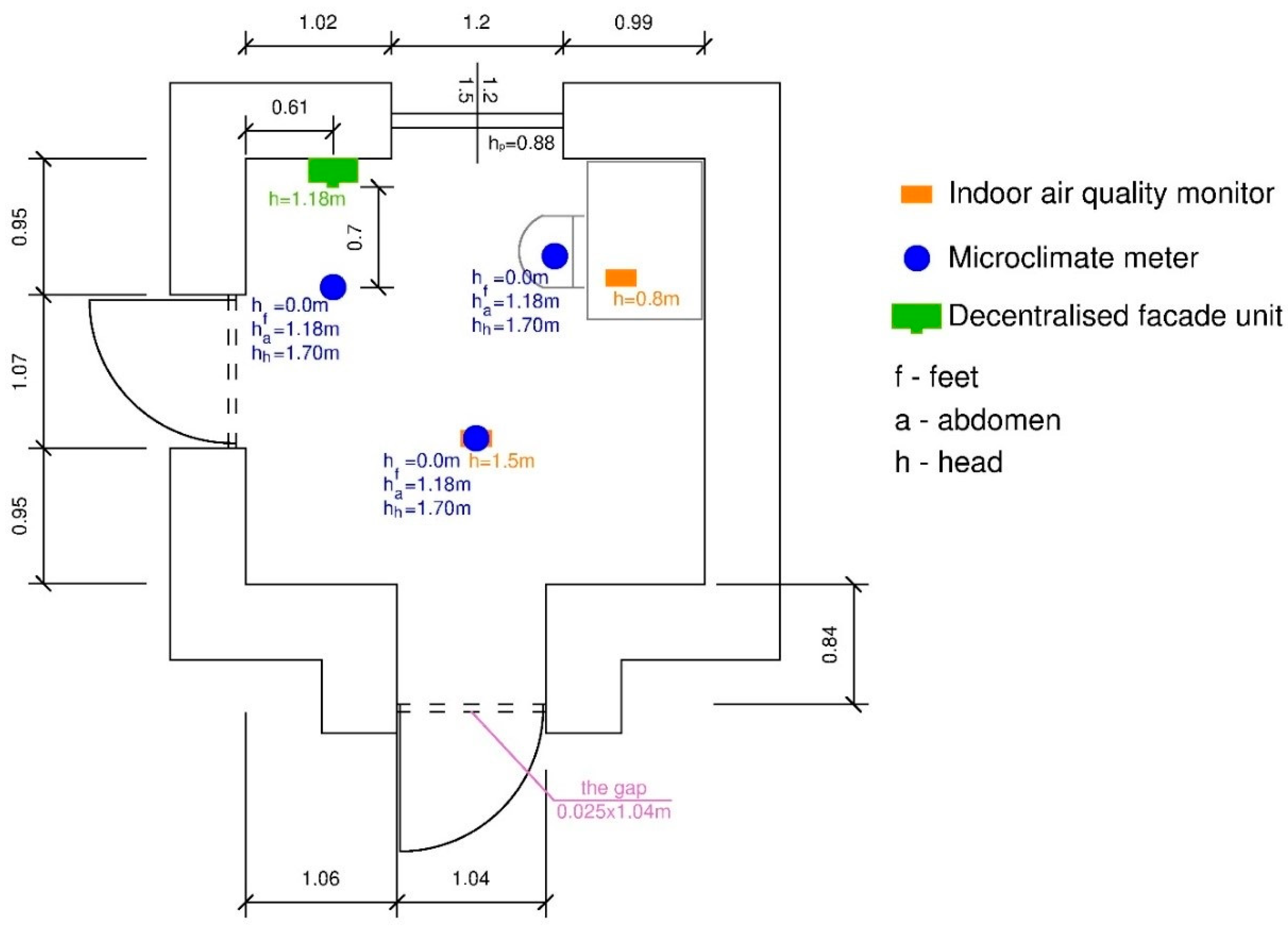
The analysis covered an office room (Figure 1) sized 2.97 m × 3.21 m × 3 m, designed for two people. The building was located in Poland in a moderate climate zone with low winter temperatures and high summer temperatures. The outdoor air temperatures characteristic for this location and at the season are within −20 to +10 °C. During the tests, the outdoor air temperature ranged from −9 to +10 °C. The heating system was deactivated in the analyzed room. Measuring equipment was located in the workplace and at the central point of the room. The room was equipped with a decentralized façade unit that was cyclically supplying and removing air from the room. During the supply cycle, air was drawn from the outside and delivered by the unit to the room, and then removed through a gap in the bottom part of the internal door. During the exhaust cycle, air was removed through the unit, and supplied via the gap in the internal door. A temperature of 21 °C was maintained in an adjacent room. The air supplied by the unit had the same temperature as the outside air, and the air flowing in through the door gap had the temperature of the air in the adjacent room.
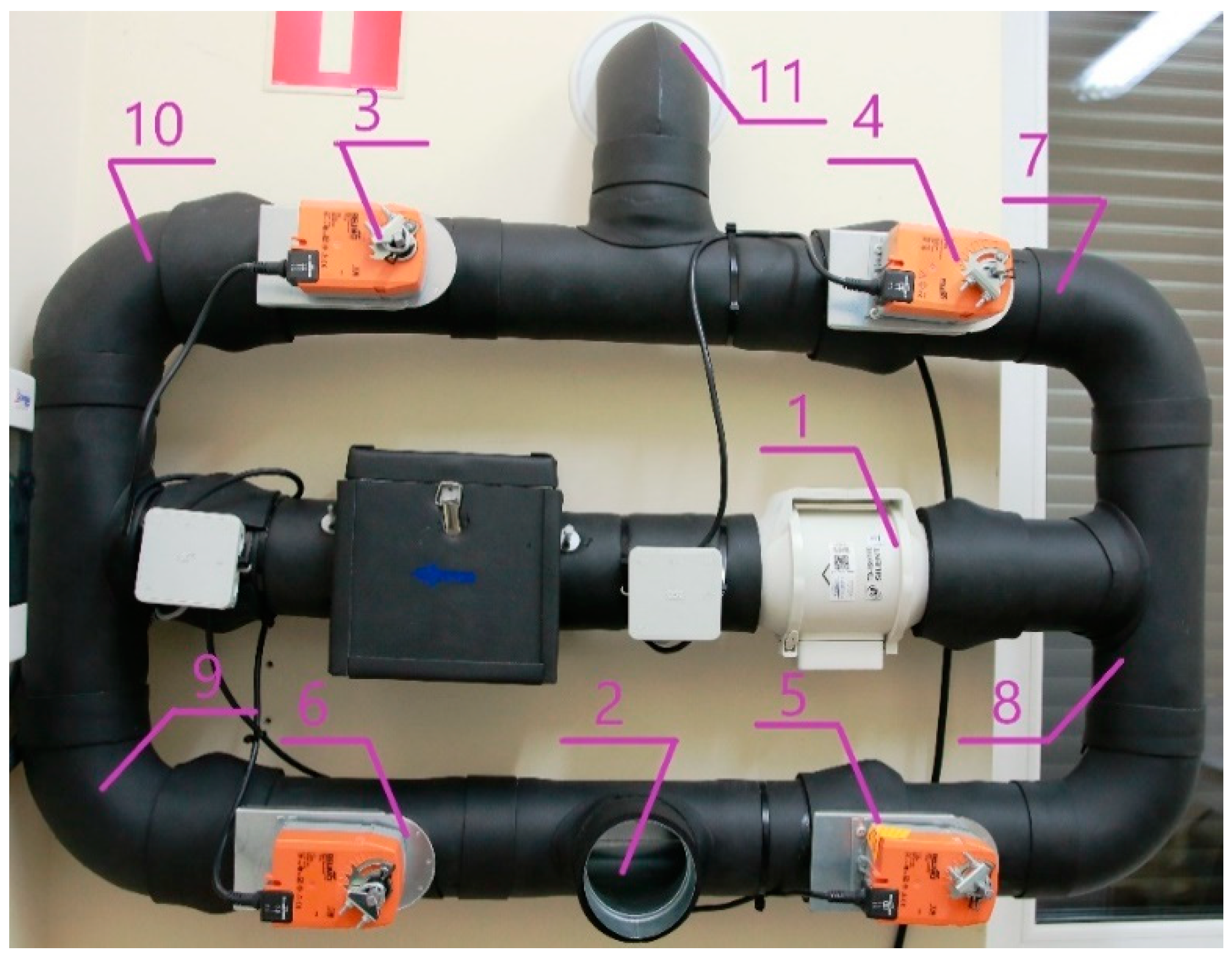
The decentralized façade unit (Figure 2) was equipped with one fan (1) pumping air continuously in one direction, and the alternation of cycles was effected by dampers (3–6) opening and closing in pairs. Air flow route was dependent on the damper opening. Dampers 4 and 6 were open during the supply cycle, and dampers 3 and 5 were open during the exhaust cycle. During the supply cycle, the air flowed through sections 7 and 9, and during the exhaust cycle, through sections 8 and 10. Component no. 2 is an intake vent/exhaust vent, and no. 11 is the air-intake/air-exhaust.
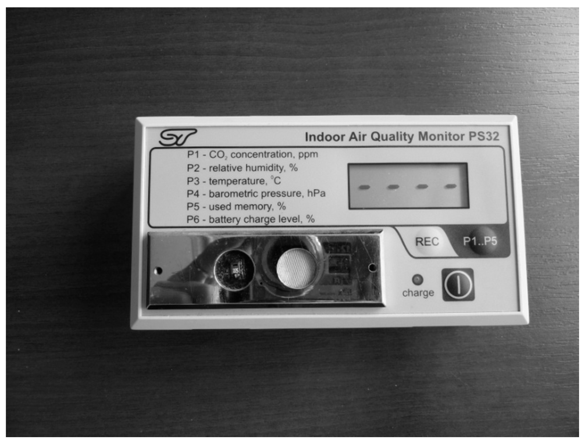
Air temperature and humidity was measured in the room and outside. The research took 26 weeks during the fall–winter–spring seasons (from November to March). The period was divided into a two-week series, during which the measurement was performed continuously every 10 s. During the experiment, the unit setting was 2 min for eight weeks, 4 min also for eight weeks, and 10 min for 10 weeks. This research period was selected because the measurements were carried out in rooms used in real conditions (in summertime users often open windows, which considerably affects the results). Two air quality meters from Sensotron (Kozielska Street 63/5, Gliwice, Poland) were used for the tests (Figure 3). Table 1 shows their measurement ranges and resolutions of indications. The instruments were set in the room user’s workplace (on the desk) 0.8 m above the floor (point 1) and at central point of the room 1.5 m above the floor (point 2). In Figure 1, the green color indicates the location of the air supply/exhaust hole; orange indicates the locations of indoor air quality monitors; blue shows the locations of the microclimate meters; and purple represents the locations of the gap in the inner door. Figure 1 also shows the heights of the places of the measurements.
The air velocity in the room was measured using a microclimate meter equipped with three anemometers (Table 2). The measurement was carried out at three points: at the workplace, in the central point of the room, and 70 cm from the supply/exhaust grate. The air velocity was measured at three levels: feet, abdomen, and head.
The values of the outside parameters (temperature and humidity of the external air) were recorded by a weather station located on the roof of the building. Table 3 presents the weather station specifications.
The amount of the supply/exhaust air and the supply/exhaust air velocity was measured using a balometer (Table 4).
The room ventilation unit was worked in three cycles with different air supply/exhaust duration: 2 min, 4 min, and 10 min. The time can be set in the range of 1 min to 10 min, thanks to the use of an actuator in the installation that closed and opened the dampers. The selected cycle lengths were dictated by the desire to show the differences in creating the microclimate at different settings of the device. One cycle consisted of successive air supply and exhaust. In the case of a 2 min cycle, the supply duration is 2 min. After this time, the actuator opens the closed dampers and closes the opened ones. The device switches to the exhaust air function, which also lasts 2 min. The same is applied for each time setting.
Statistical Analysis
The unit work was evaluated from the statistical point of view. The two-factor ANOVA with replication and the Tukey multiple comparison method were employed for this purpose. Determinants for the group of comparisons included setting (air supply/exhaust duration), measuring instrument location, outside temperature, and outside humidity.
3. Results and Discussion
3.1. Experimental Studies
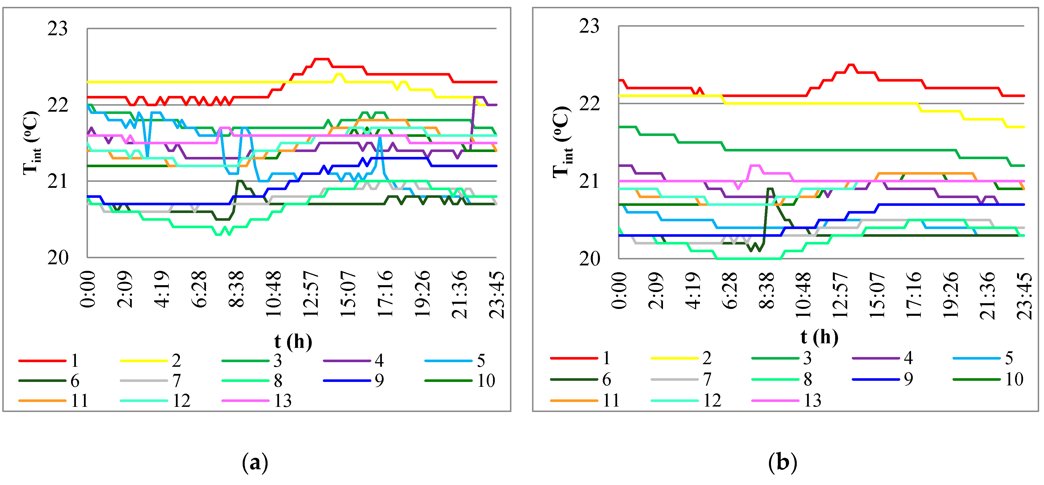
The air temperature measured with a 10 s step allowed for the average value for each hour for a two week period to be calculated. The average air temperature values calculated for different points of the room proved to be insignificant fluctuations at different outside air temperatures.
Figure 4 shows the average air temperature values measured at two locations in the room during thirteen two-week periods. Each line corresponds to the daily changes in the average air temperature. Each point corresponds to the mean calculated for each hour of the day from the two-week measurement period. The trajectory of changes in the analyzed parameter in time show minor daily temperature fluctuations in each of the two measurement points. During periods 1–4, the duration of the air ventilation unit supply/exhaust cycle was 2 min (2 min for air supply, and the next 2 min for air exhaust); during periods 5–8, it was 4 min; and during periods 9–13, it was 10 min.
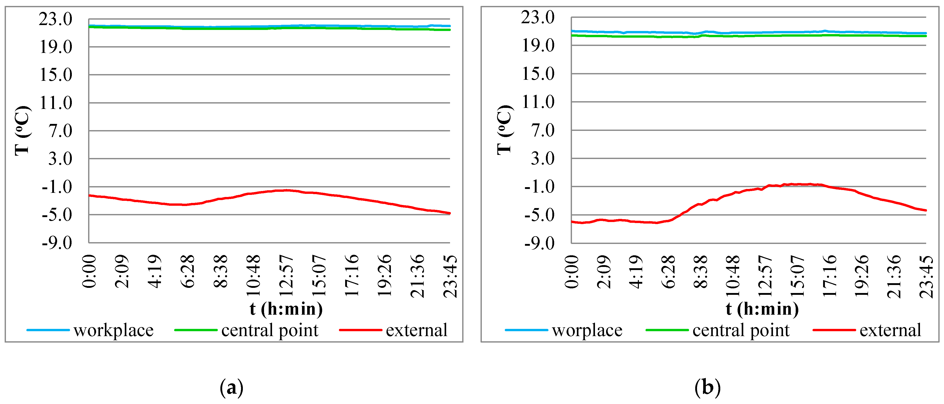
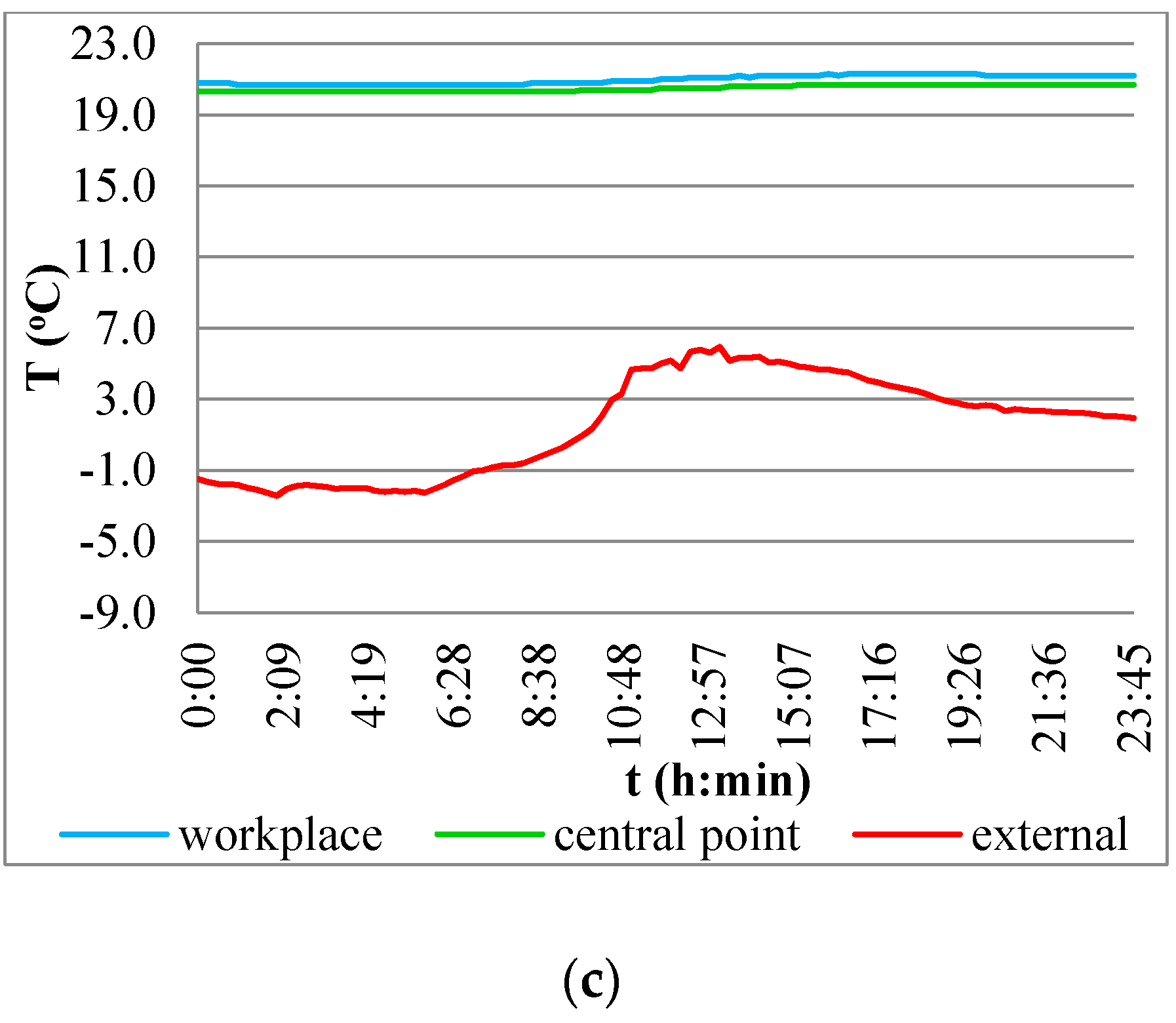
An average of the values of measured temperature for a given hour in a day was calculated for each of the cycles, and inside air temperature values were compared to the outside air temperatures (Figure 5).
Temperature analysis proved that the values obtained for the workplace and central point of the room satisfied thermal comfort requirements according to the PN-EN 16798-1:2019-06 standard [39], despite the different values of outside air parameter. No influence of outside air temperature on room chilling was observed.
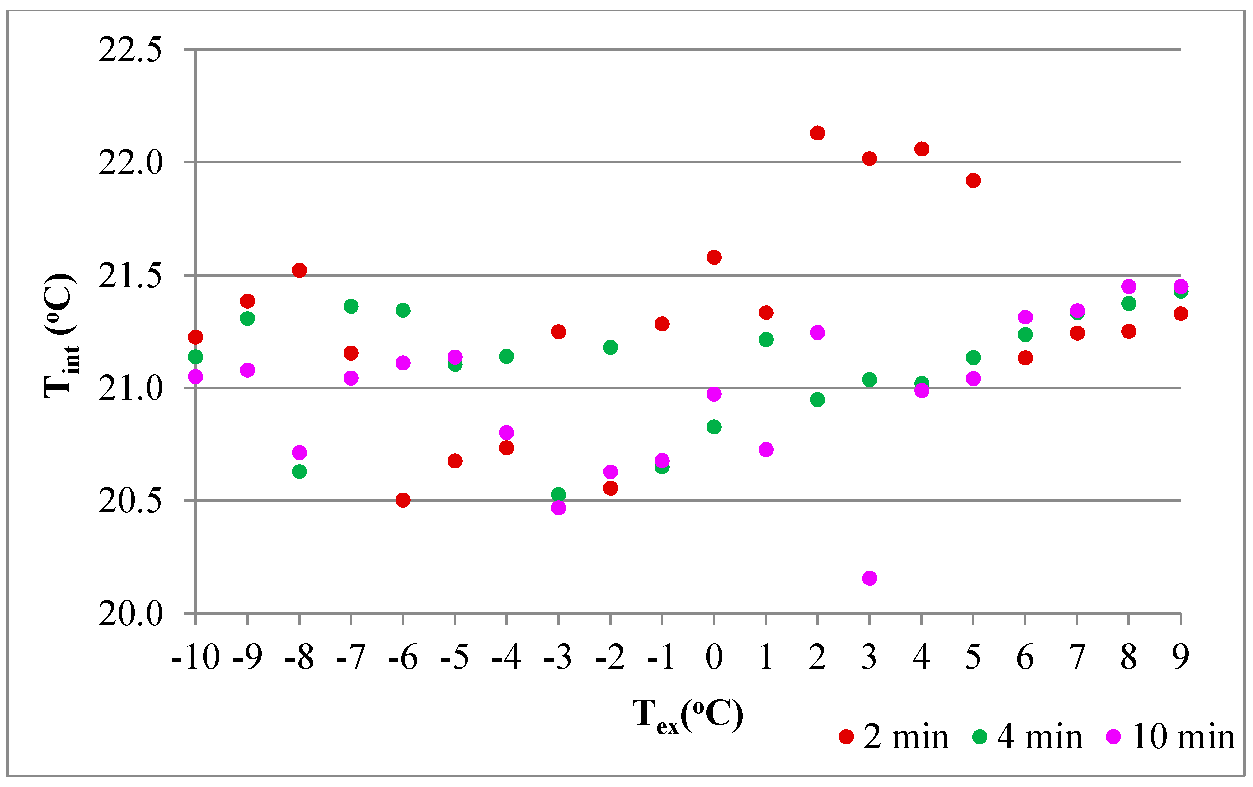
The next step involved the analysis of inside air temperature dependence on outside air temperature. Figure 6 demonstrates the obtained results and analyzed whether air supply/exhaust duration would affect the temperature value. The inside air temperature remained within the thermal comfort range throughout the measurement period. The average of the recorded temperature values ranged from 20.2 °C to 22.1 °C, which means that despite supplying low temperature air and regardless of air supply process duration (2 min, 4 min, 10 min), the temperature in the room was stable.
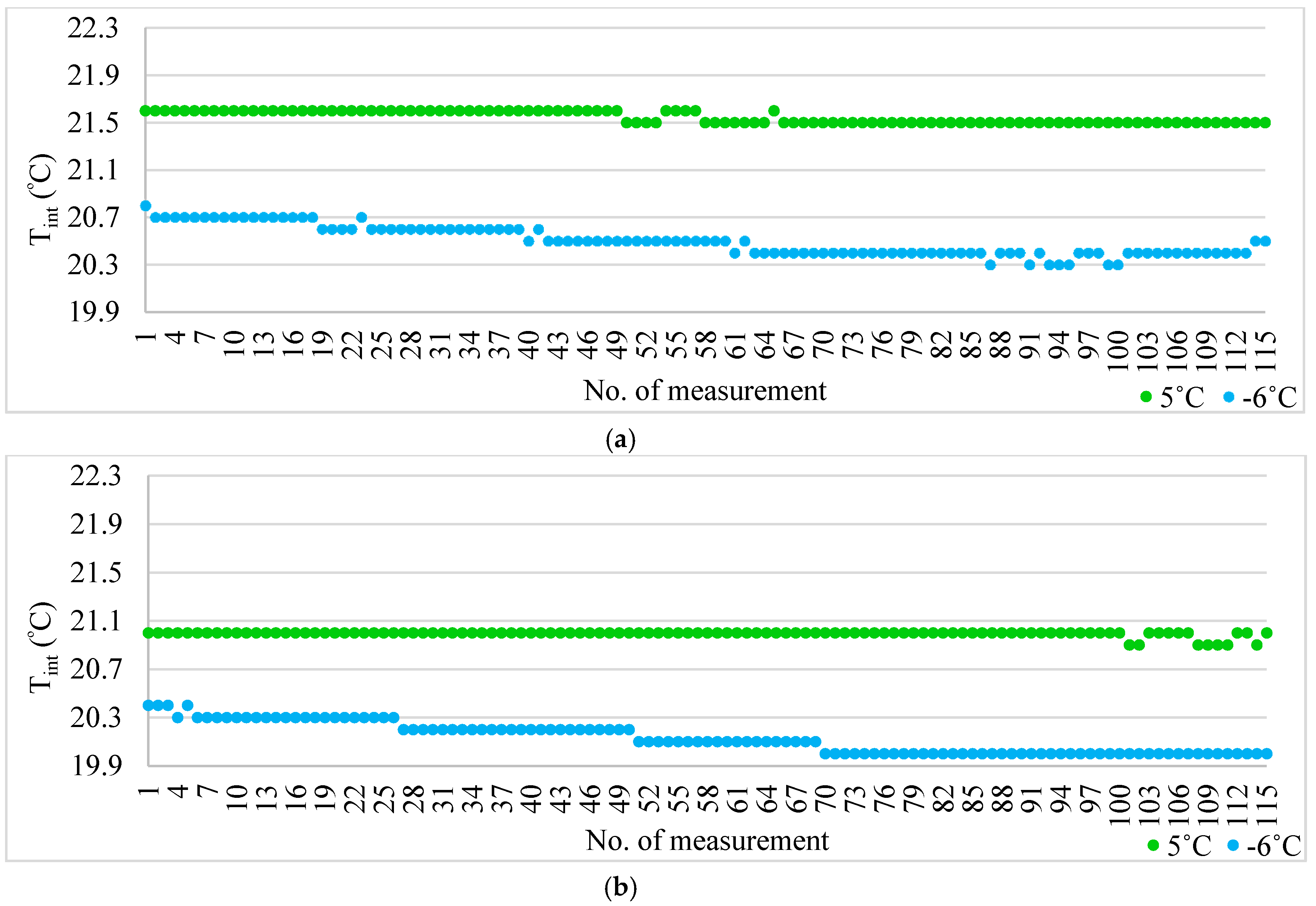
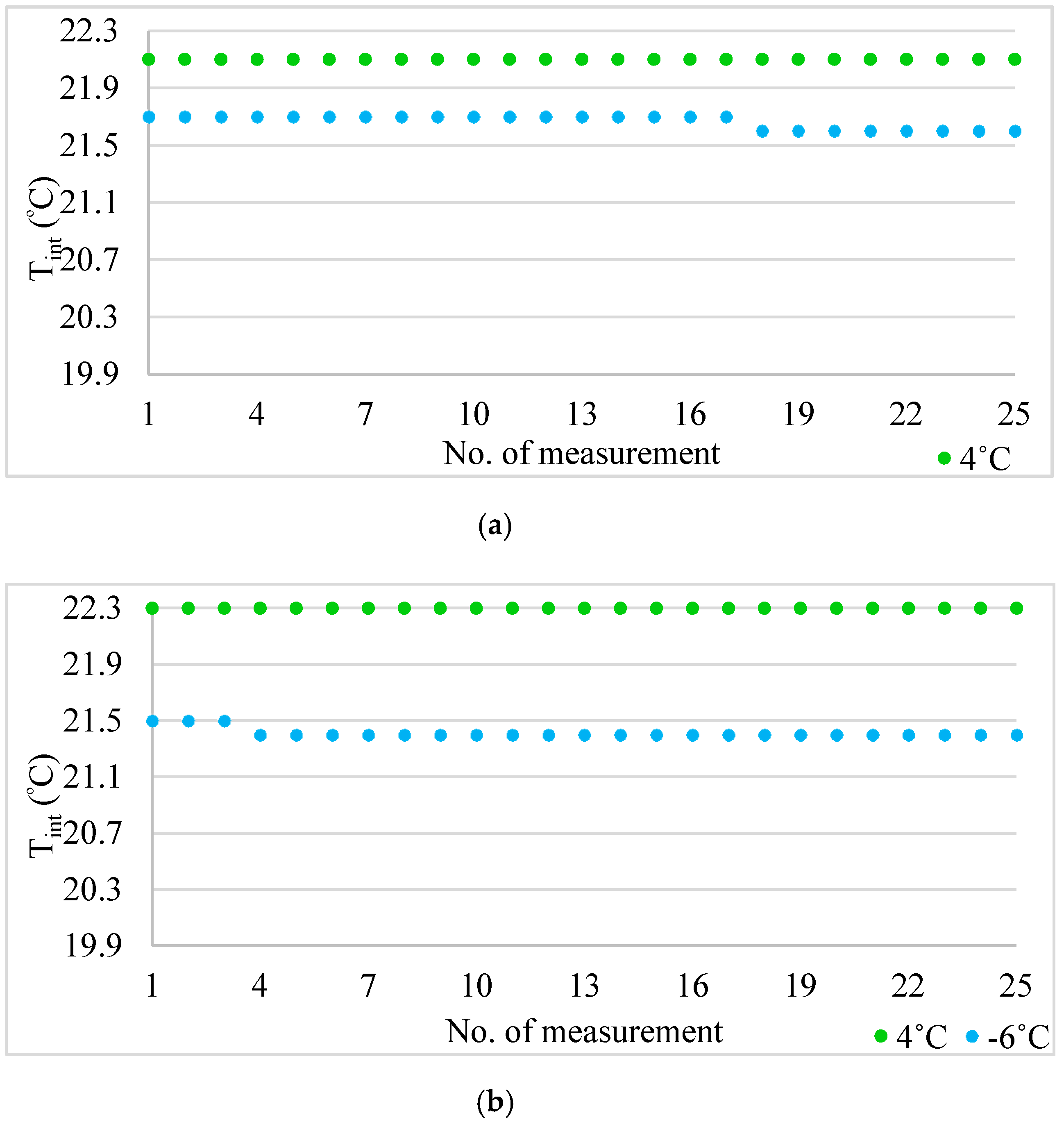
Both in the shortest cycle of 2 min and the longest cycle of 10 min, the values of internal air temperature met the requirements of thermal comfort (Figure 7 and Figure 8). The thermal comfort temperatures inside the room were maintained both at the outside air temperature of 4–5 °C and the temperature of −6 °C. At the same time, the temperature of the inside air was lower in the case of the negative values of the outside temperature, but also in this case the values met the comfort requirements.
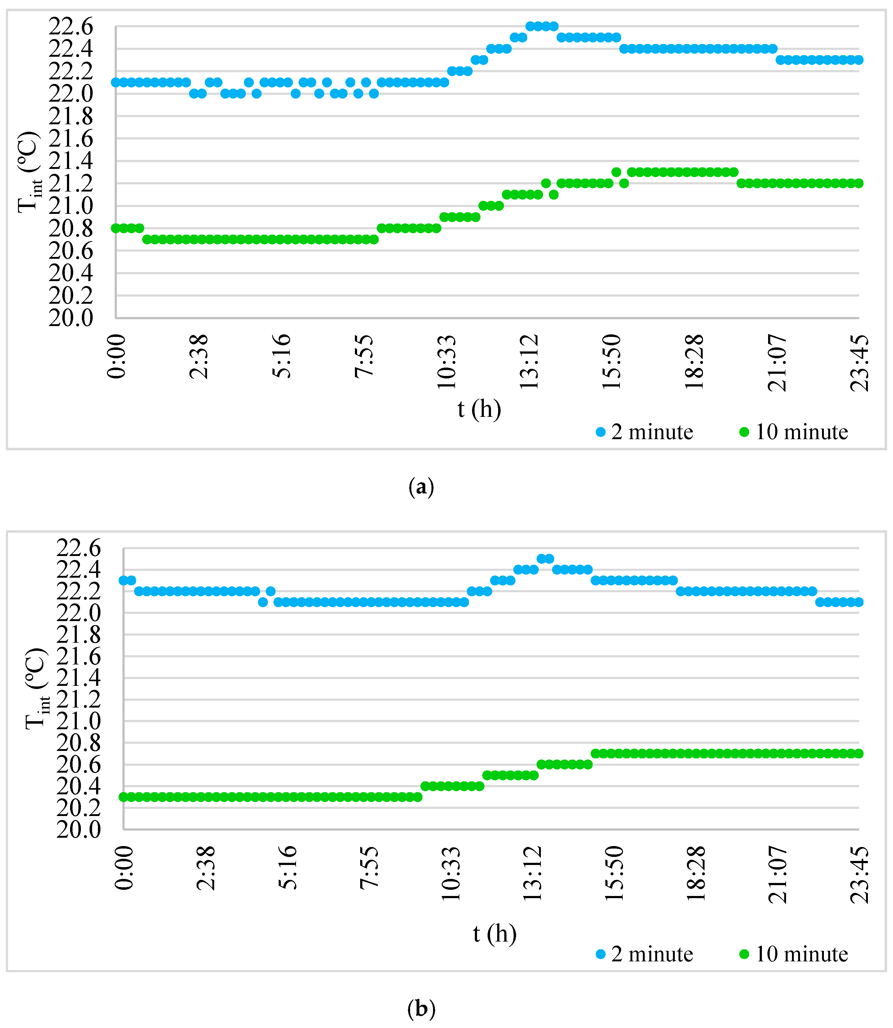
Examples of days with similar external conditions (temperature −2 ± 4 °C and humidity 80–90%) were selected from the measurement data. Figure 9 shows the course of the temperature changes over time for two locations of the meters: the workplace and the central point of the room. In both cases, the room met the requirements of thermal comfort regardless of the duration of the cycle. At the same time, the temperatures were lower for the longer cycle than for the shorter.
Average air humidity values measured at different locations in the room proved to be minor fluctuations.
Figure 10 demonstrates the fluctuations of the average air humidity values over time.
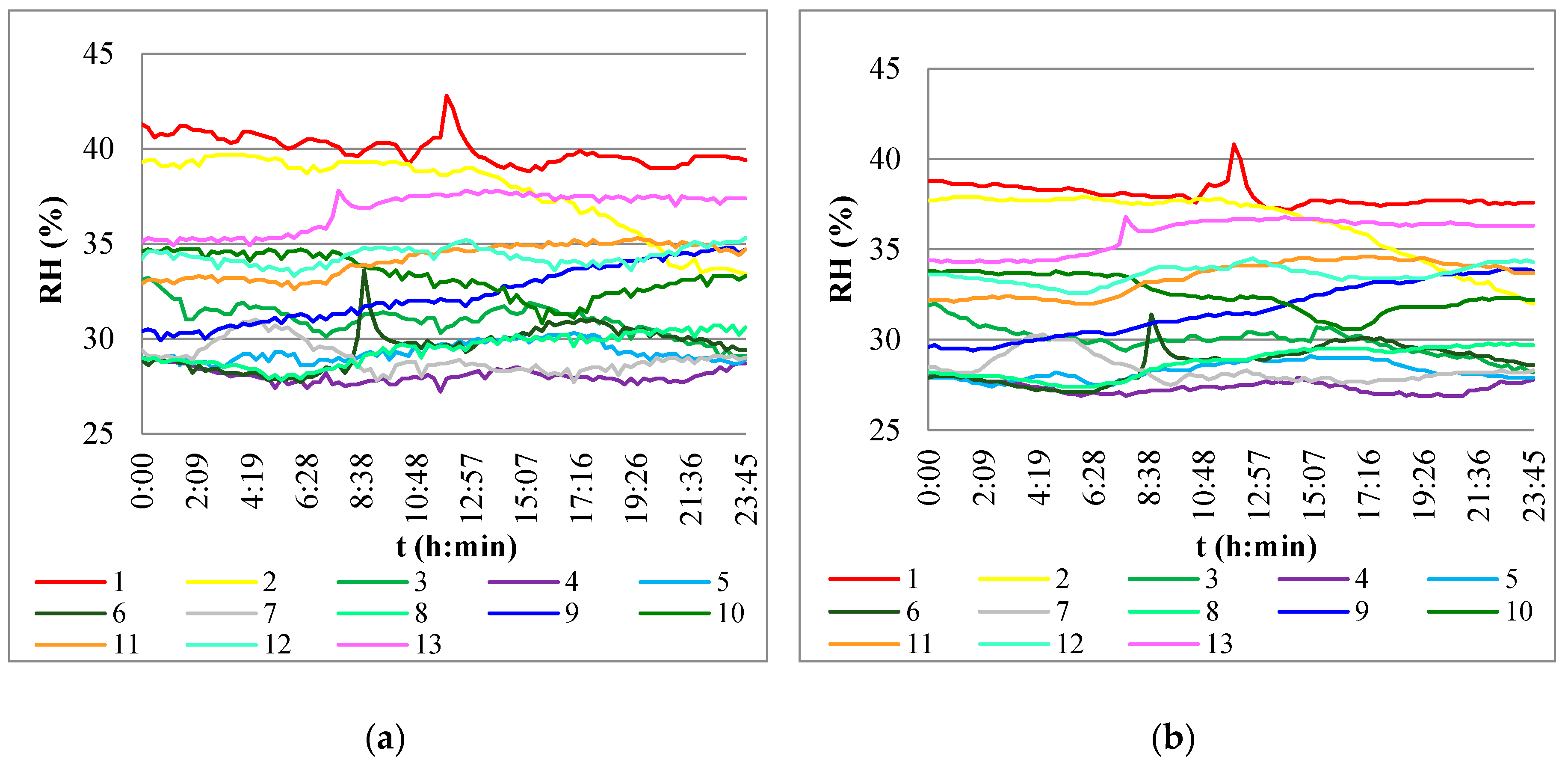
Inside air humidity values were compared to outside air humidity in each of the thirteen measurement periods (Figure 11).
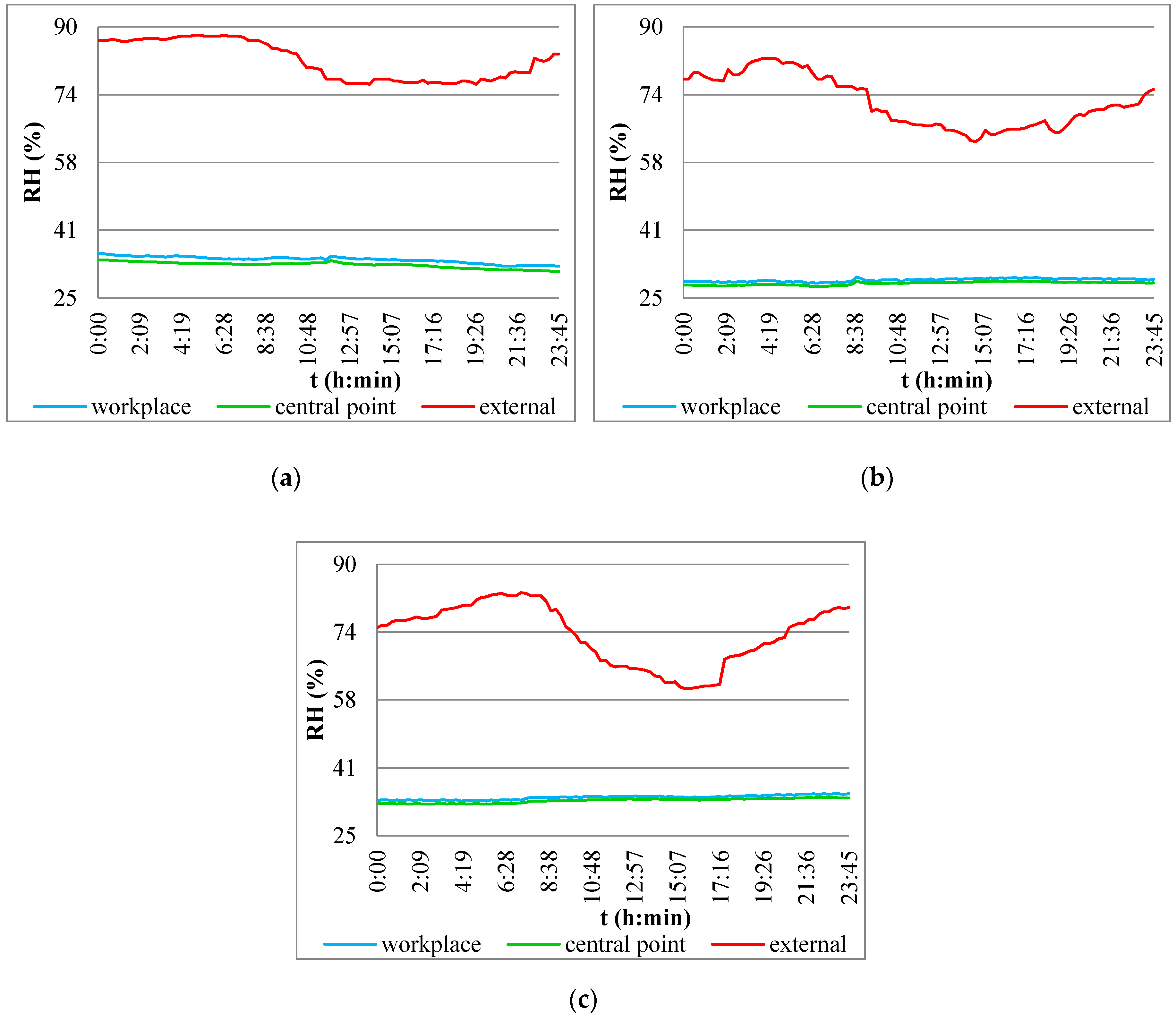
Air humidity analysis proved that the values measured in the room did not always satisfy thermal comfort requirements according to the PN-EN 15251:2012 standard [40]. The decrease in the relative humidity in the room was observed when the outside temperature was low and the external relative humidity was high.
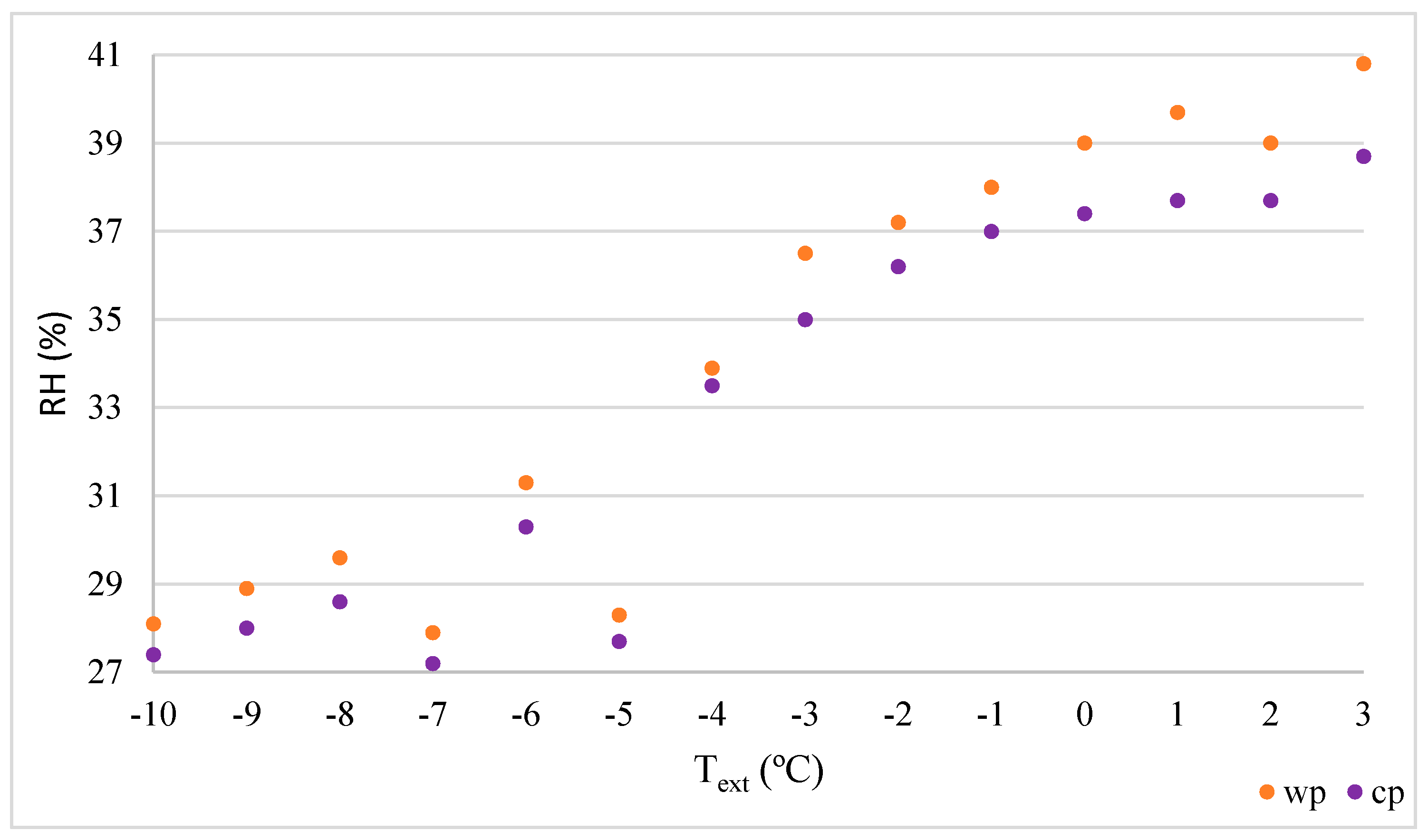
Figure 12 shows the relationship between the relative humidity of the indoor air and the temperature of the outdoor air. An increase in the indoor air humidity, along with an increase in outdoor temperature was demonstrated. Moreover, when the external temperature equaled −10 to −5 °C, the indoor air humidity did not meet the requirements of thermal comfort in accordance with PN-EN 15251:2012 [40]. At the same time, the difference between the relative humidity at the two measurement points was small.
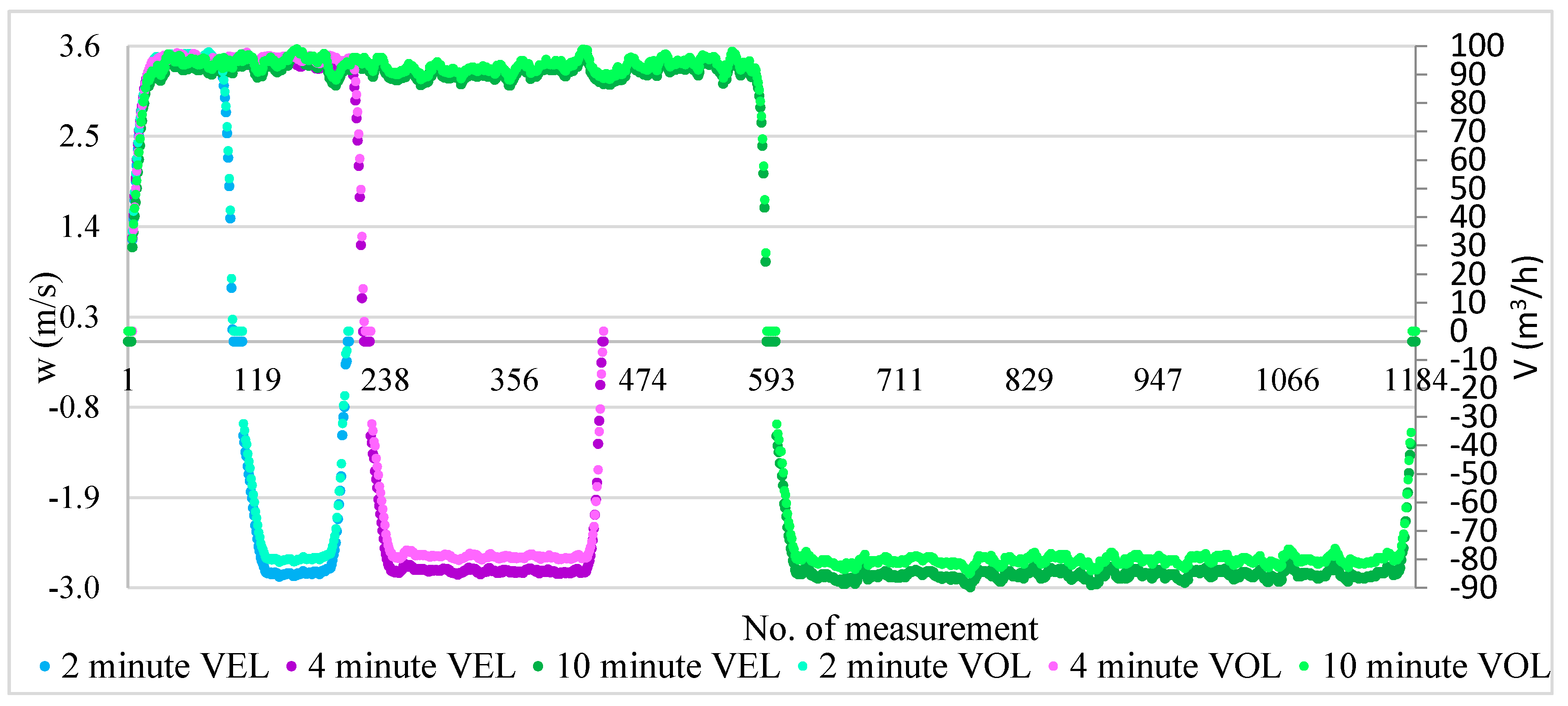
The device effectiveness was assessed on the basis of measurements of the supply air velocity and the level of carbon dioxide concentration. The velocity and the supply air stream were measured for each of the analyzed cycles (Figure 13). The measured values made it possible to determine the air change rate, which was 2.3 h−1 for the shortest cycle, and 2.7 h−1 for the longest cycle. For comparison, devices with heat recovery exchangers and reversible fans [41] exchange the air with an air change rate of 0.18 h−1. This could be a sufficient value for living quarters, but for an office room, the number of air changes should be higher.
The literature [42] shows the influence of the pressure difference inside and outside the building on the speed of the supplied air, and thus the amount of air. In the case of the presented analysis, the focus was on measuring the air velocity and amount of air flowing into the room without analyzing the impact of wind conditions on the work of the device.
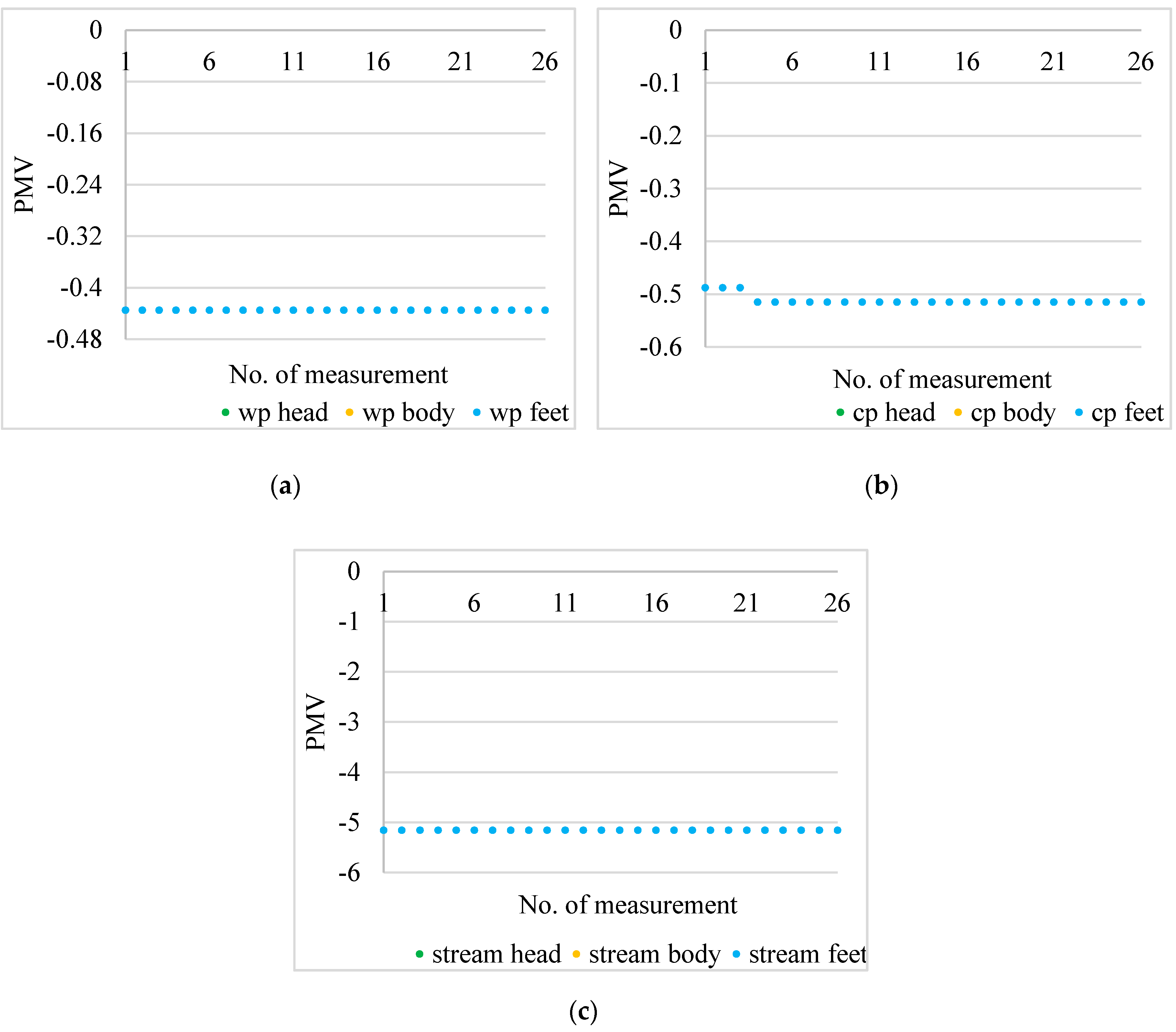
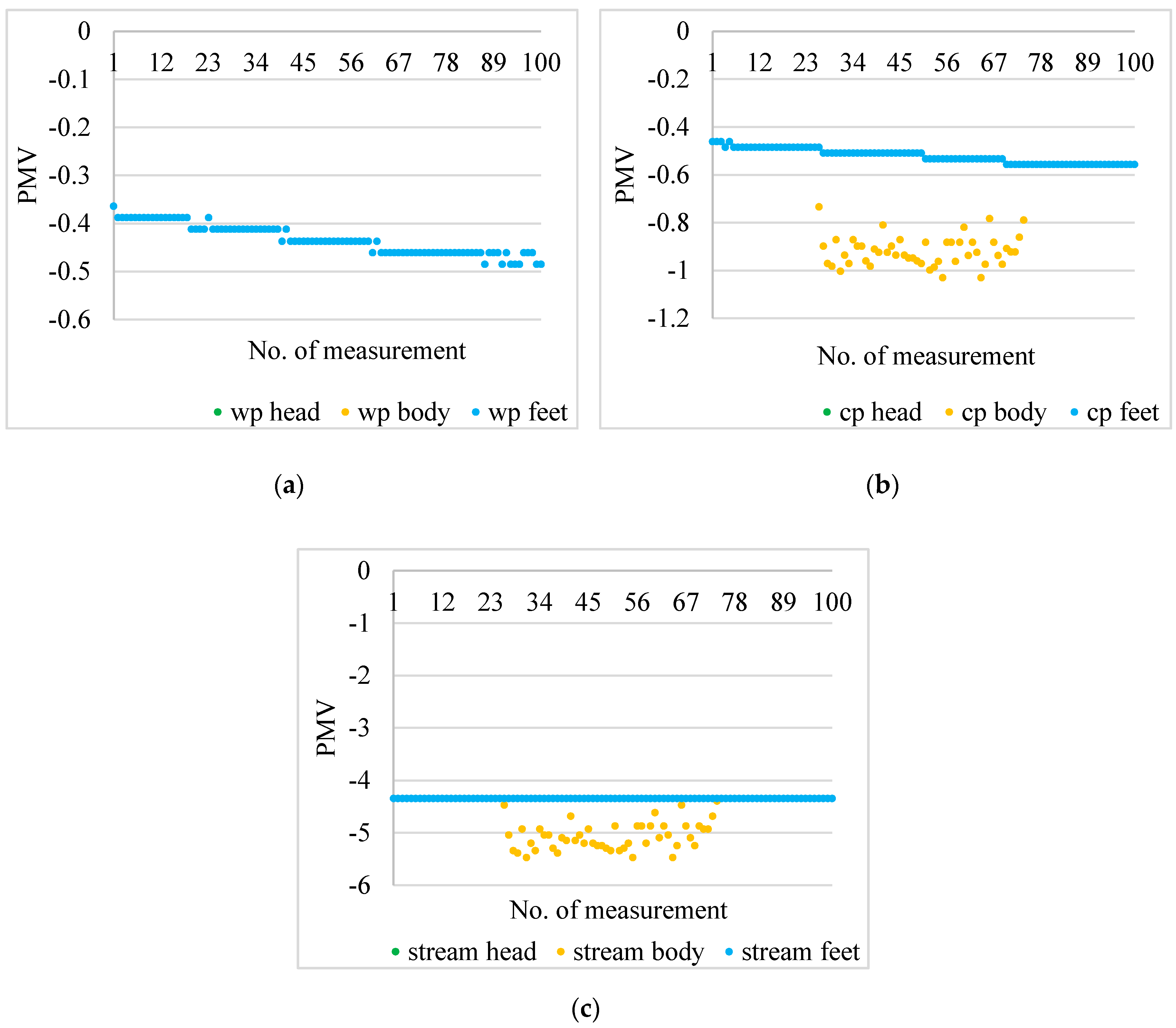
The air velocity was also measured within the room at three levels: the feet, abdomen, and head. The measurement was carried out in the workplace, at a central point, and at a distance of 70 cm from the supply/exhaust grate. The performed measurements made it possible to calculate the PMV index (predicted mean vote) in accordance with the PN-EN 7730 [43] standard (Figure 14 and Figure 15).
On the basis of Figure 14 and Figure 15, it can be seen that in the area of the head, abdomen, and feet, the workplace belongs to the category of room B, according to the classification of the standard PN EN 7730 [43]. The central point of the room was in category C at the end of the cycle (2 min). In the long cycle (10 min), it belonged to category C for almost the entire duration of the airflow (at all parts of the body). Additionally, the DR (draught rating) was calculated, which defines the percentage of people dissatisfied with the air movement. The analysis showed that in the case of the longest cycle (i.e., with a supplytime of 10 min), for half the time of supply (5 min), in the center of the room at the level of the abdomen, 13–20% of people were dissatisfied with the draught. However, users did not experience any draught in the area of the feet and head, so there will be no feeling of draught at every level of the body in the workplace location. However, at a distance of 70 cm from the supply/exhaust grate at the level of the abdomen, the air movement was strongly felt and the DR was from 37 to 64%. For this location, there was no feeling of draught at the levels of the feet and head. For a 2-min cycle, the index was 0 for all locations and all body parts, which means that there will be no dissatisfied people with the draft.
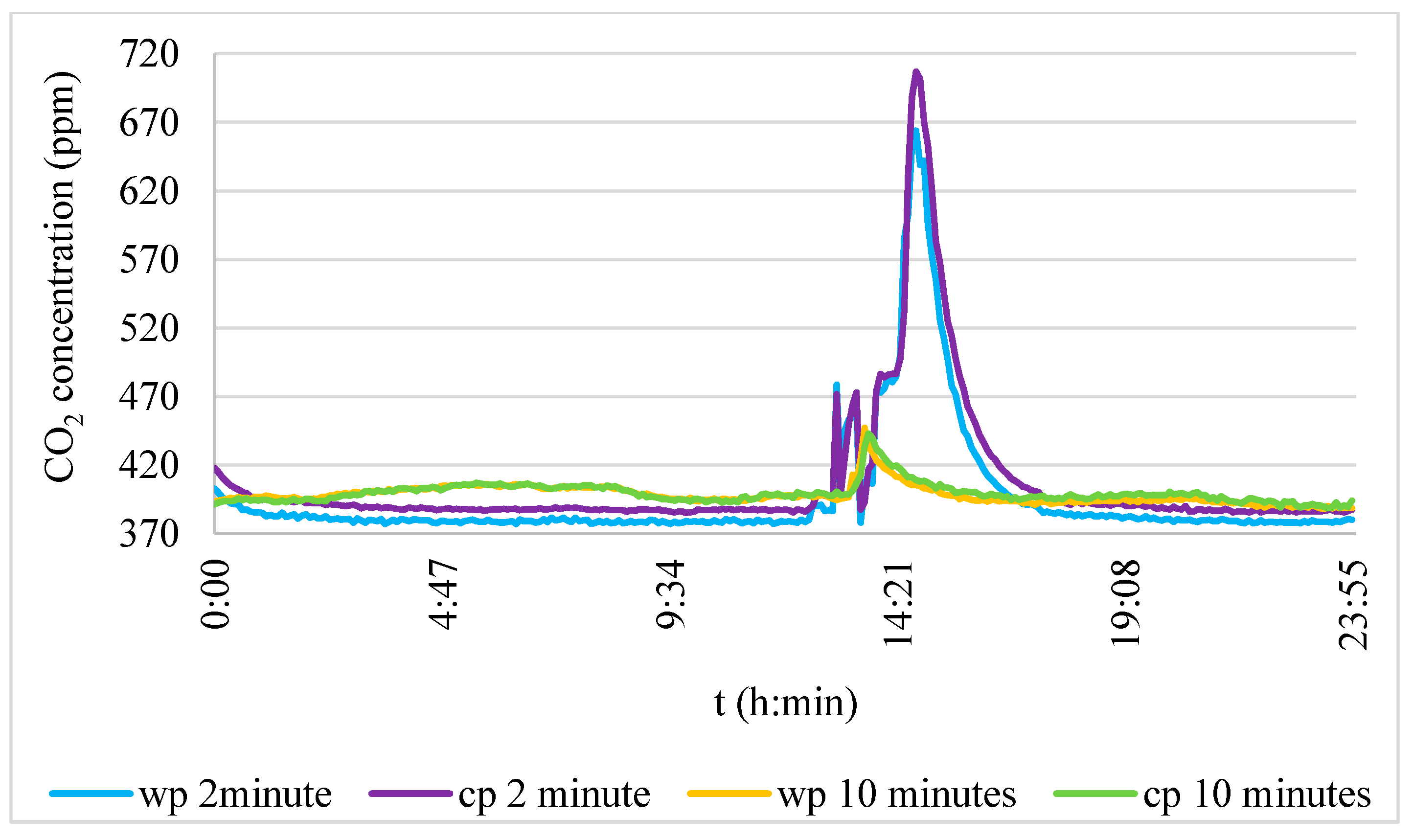
In the literature [44], there are efficiency analyses of decentralized devices equipped with two fans. For the efficiency assessment, we used the level of carbon dioxide concentration and radon concentration in the room. The analysis showed that the decentralized devices diluted the gaseous pollutants sufficiently. In the presented case, the measurement of carbon dioxide concentration also showed (Figure 16) that the façade device sufficiently exchanged the air for fresh air.
The results are presented for an example day. There was a visible increase in the concentration of carbon dioxide upon entering the user’s room. At the same time, with a longer supply/exhaust time (10 min), the maximum value of the carbon dioxide concentration was lower than for the short cycle (2 min). For each cycle length, throughout the entire period of measurements, the concentration of carbon dioxide did not exceed the value of 800 ppm, which means that the room met the ASHRAE [45] requirements for air quality in offices.
3.2. Statistical Analysis
Measured data were used to carry out the statistical analysis of the unit operation. The two-factor ANOVA was carried out for the temperature characteristic. The grouping variables were: setting with values of 2, 4, and 10 min, and location with values: wp (workplace) and cp (central point).
The zero hypotheses stating equality of the average values of the temperature characteristic was verified on the basis of all combinations of levels for both equivalent factors and the F statistic was used for this purpose (the ratio of intergroup variance to intragroup variance). Table 5 contains the results of completed calculations used to verify the hypothesis stating equality of the average values of the temperature characteristic in groups determined on the basis of both factors.
A value p obtained for statistic F in a completed test of less than 0.0001 allows for the statement that there were at least two groups where the average values of the temperature characteristic differed.
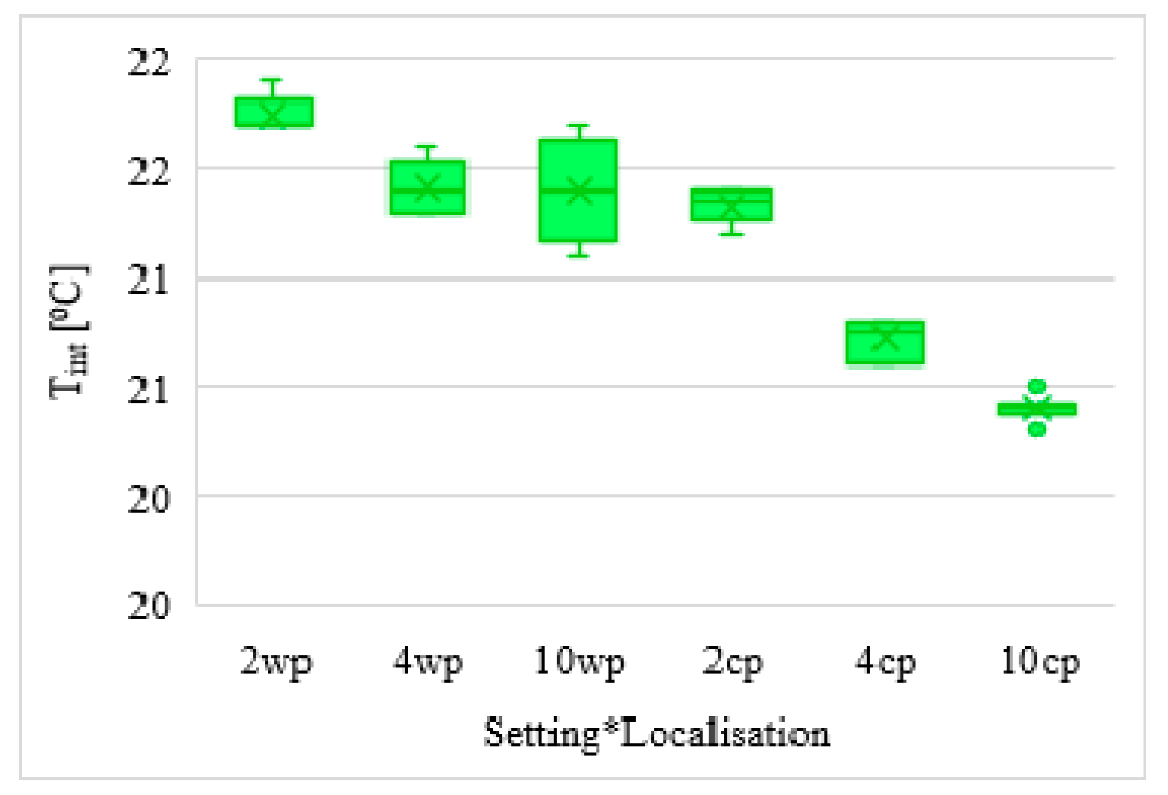
Figure 17 demonstrates in box plots the significance of the effect of the interactions between the factors. The distribution of the temperature characteristic in groups defined by setting and location factors is illustrated in this way.
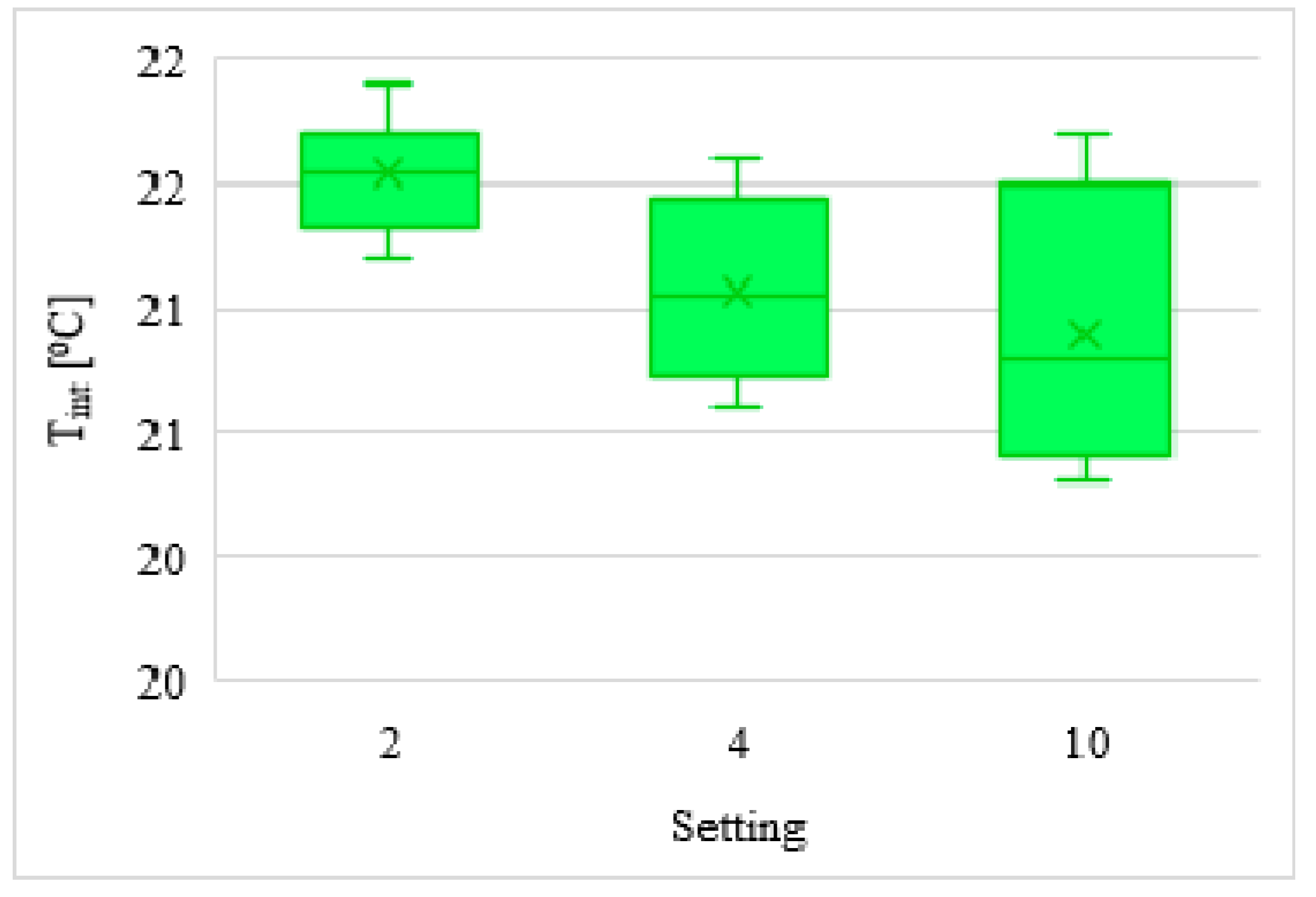
Figure 18 shows box plots illustrating the distribution of the temperature characteristic in groups defined by the setting factor levels.
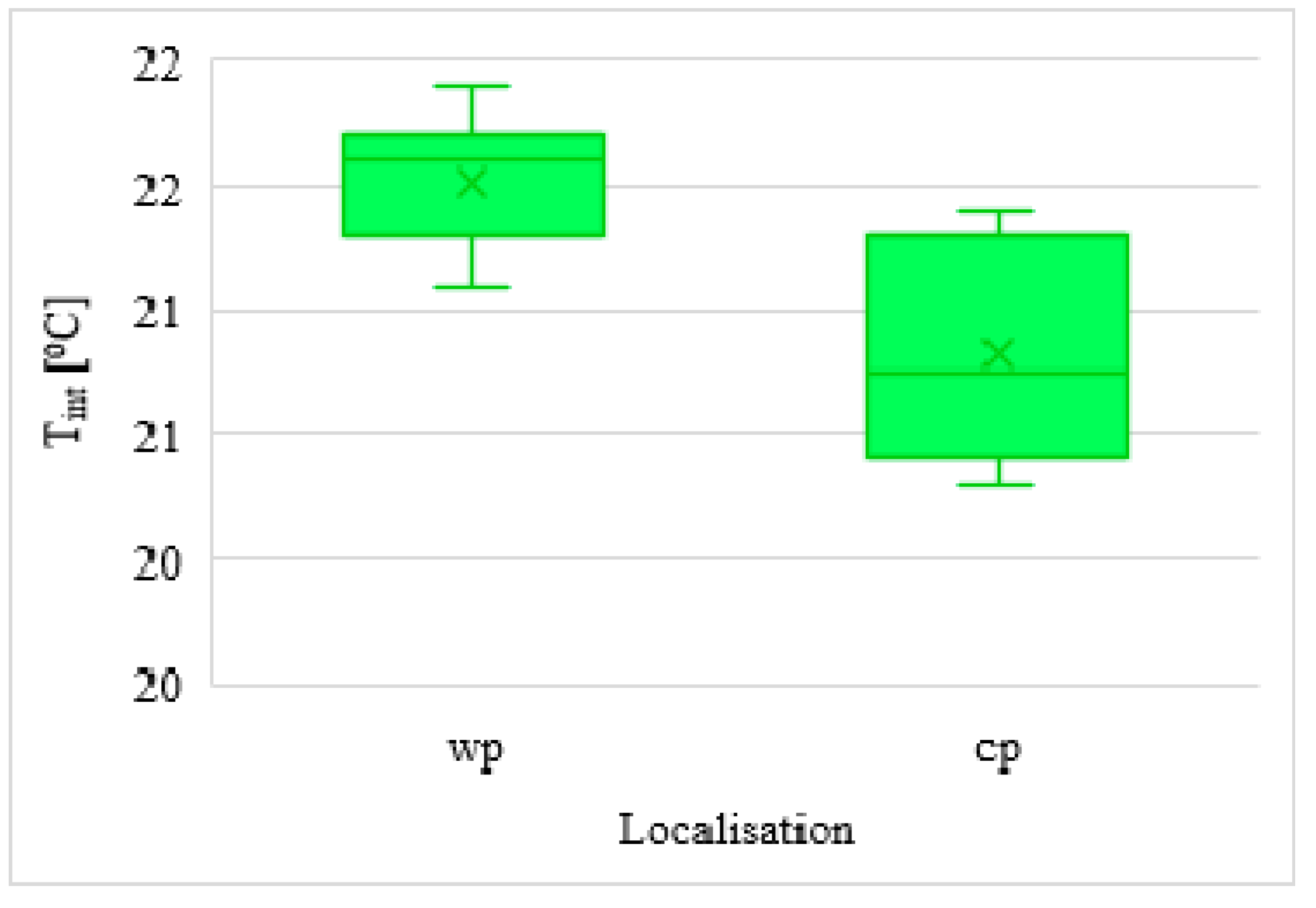
Figure 19 shows box plots illustrating the distribution of the temperature characteristic in groups defined by location factor levels. A statistically significant main effect was observed both for setting and for location. Thus, it is well-grounded to apply the Tukey multiple comparison method.
Table 6 contains the calculation results for the temperature characteristic, carried out according to the Tukey method in groups matching the levels of 2, 4, and 10 min of the setting factor.
Table 6 shows that the highest average temperature value should be expected for the 2 min setting and the lowest for the 10 min setting.
The data in Table 7 confirm the conclusions derived from Table 6. None of the achieved 95-percent confidence intervals included zero, which means that the differences between average temperature values for each of the pairs were statistically significant. There is a possibility of the quantitative determination of the differences between average temperature values using 95-percent confidence intervals. For example, for the difference in average temperature values in groups matching the 4 min setting and 10 min setting, the extremes were 0.02 and 0.3. Each value within the interval with specified extremes was treated equally as a potential true value of the analyzed difference. Thus, it should be accepted that an average temperature for the 4 min setting may exceed the average temperature for the 2 min setting by either 0.02 or 0.3.
Table 8 contains the calculation results for the temperature characteristic, carried out according to the Tukey method in groups matching the following levels: wp (workplace) and cp (central point) of the location factor.
Table 6 shows that the average values of the temperature characteristic in the group defined by workplace location were significantly higher than those corresponding to the central point location.
The data in Table 9 confirmed the conclusions derived from Table 8. None of the achieved 95-percent confidence intervals included zero, which means that the differences between the average temperature values for each of the pairs were statistically significant. The data allowed for the quantitative determination of the differences between the average temperature values by way of implementing 95-percent confidence intervals. For example, interval extremes for the difference in average temperature values in groups defined by workplace and central point location were 0.6 and 0.8, respectively. Each value within the interval with specified extremes was treated equally as a potential true value of the analyzed difference. Thus, it should be accepted that an average temperature for workplace location may exceed the average temperature for the central point location by either 0.6 or 0.8.
The next step involved carrying out the two-factor ANOVA for the temperature characteristic with the following grouping variables: setting with values of 2, 4, and 10 min and outside temperature with values of −7 °C and −3 °C.
The zero hypothesis stating equality of the average values of the temperature characteristic was verified on the basis of all combinations of levels for both equivalent factors. The F statistic was used for this purpose. Table 10 contains the results of the completed calculations used to verify the hypothesis stating the equality of average values of the temperature characteristic in groups determined on the basis of both factors.
A value p obtained for statistic F in the completed test of greater than 0.0001 allows to state that the average values of the temperature characteristic did not differ.
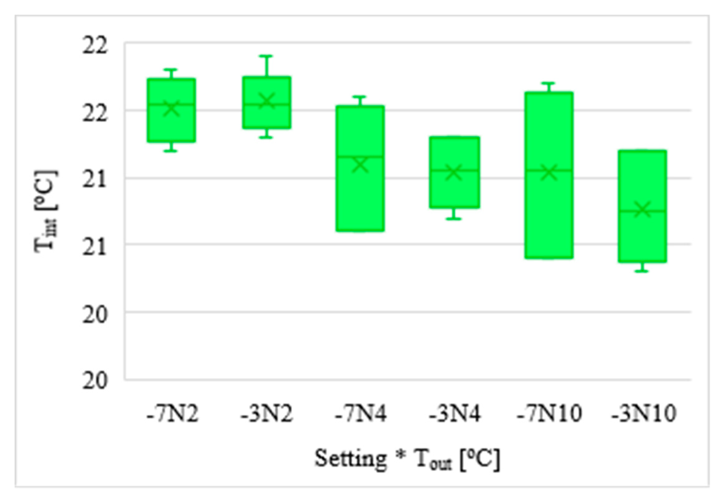
Figure 20 demonstrates in box plots the significance of the effect of the interactions between the factors. The distribution of the temperature characteristic in groups defined by setting and outside temperature factors is illustrated in this way.
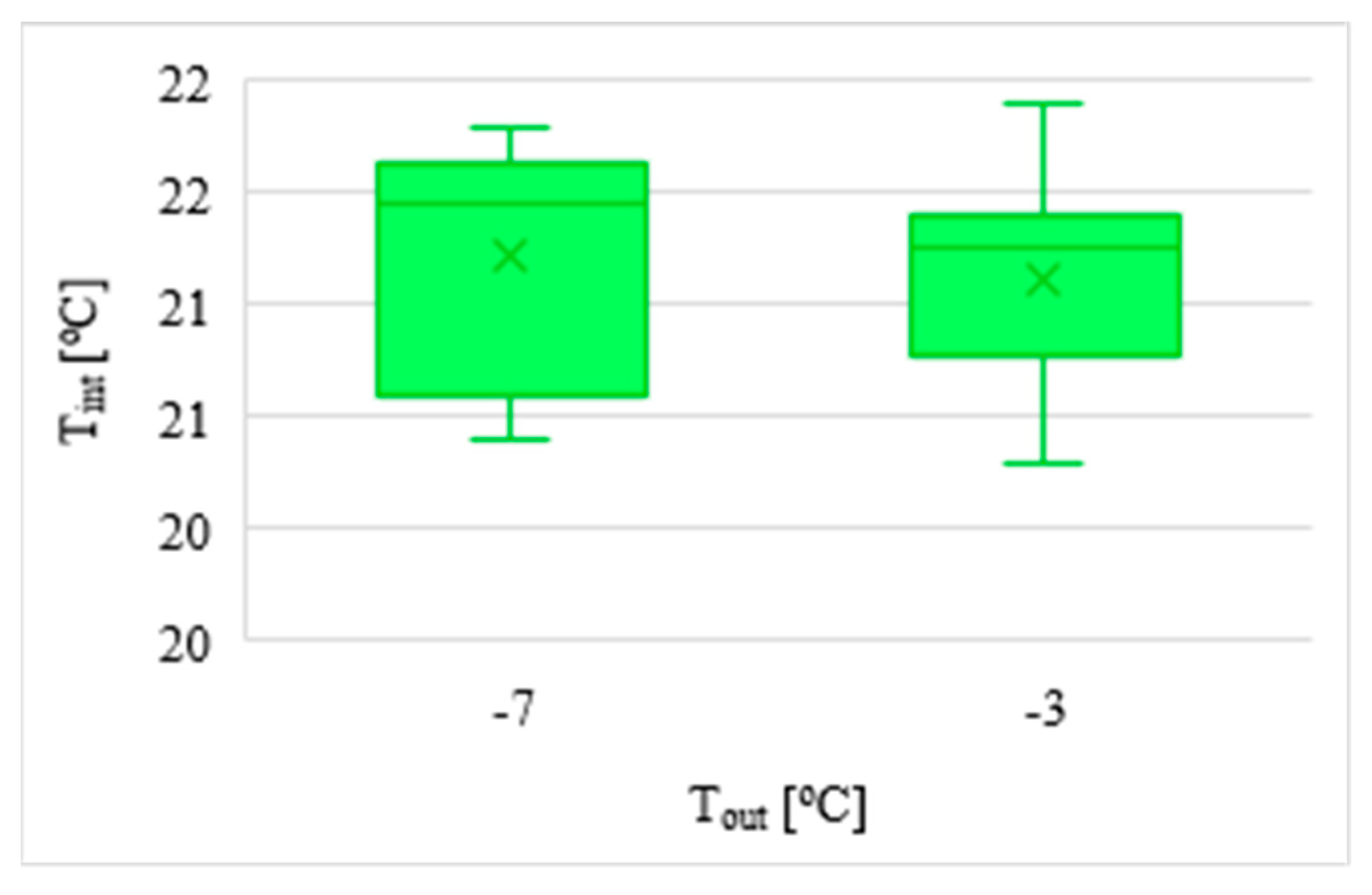
Figure 21 shows box plots illustrating the distribution of the temperature characteristic in groups defined by the outside temperature factor levels.
Table 11 contains the calculation results for the temperature characteristic, carried out according to the Tukey method in groups matching the levels of −7 °C and −3 °C of the outside temperature factor.
Table 11 shows that the average temperature values did not differ significantly.
The two-factor ANOVA for the humidity characteristic was carried out in the same way. The grouping variables were: outside temperature with the values of −10.5, −10, −9.5, −9, −8.5, −8, −7.5, −7, −6.5, −6, −5.5, −5, −4.5, −4, −3.5, −3, −2.5, −2, −1.5, −1, −0.5, 0, 0.5, 1, 1.5, 2, 2.5, and 3 °C and location with the values wp (workplace) and cp (central point).
The zero hypothesis stating equality of the average values of the humidity characteristic was verified on the basis of all combinations of levels for both equivalent factors. The F statistic was used for this purpose (the ratio of intergroup variance to intragroup variance). Table 12 contains the results of the completed calculations used to verify the hypothesis stating equality of the average values of the humidity characteristic in groups determined on the basis of both factors.
A value p obtained for statistic F in the completed test of less than 0.0001 allows for the statement that there were at least two groups where the average values of the humidity characteristic differed.
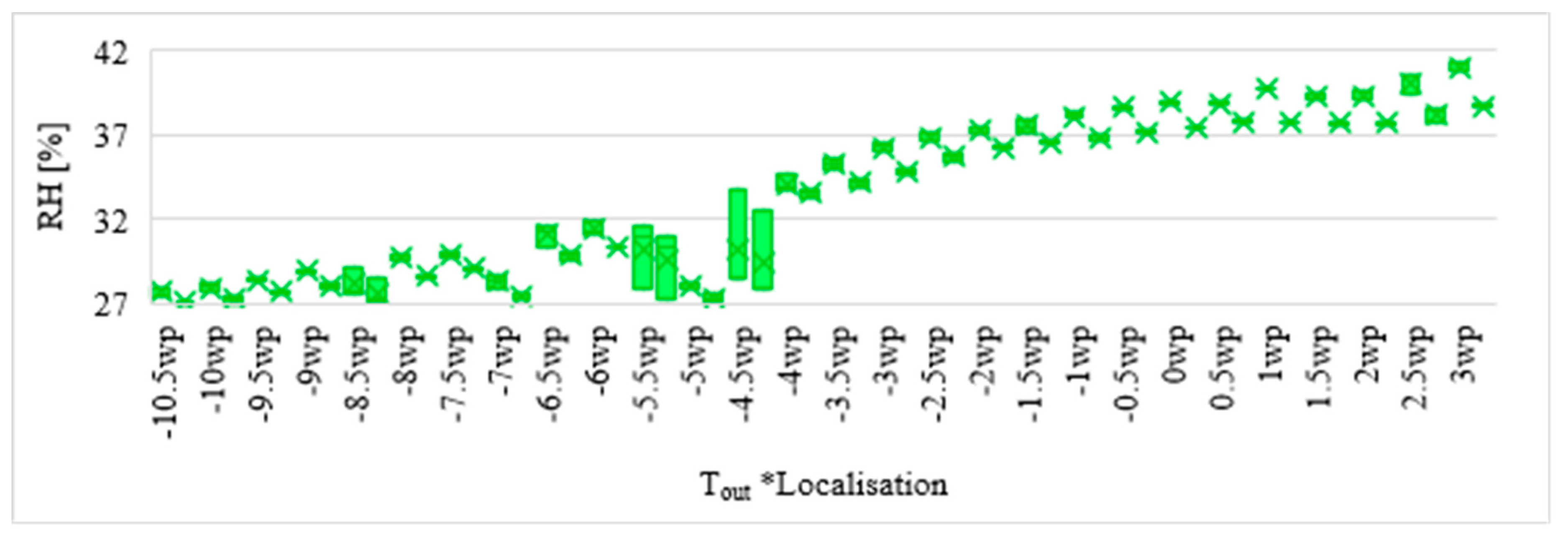
Figure 22 demonstrates in box plots the significance of the effect of the interactions between the factors. The distribution of the humidity characteristic in groups defined by outside temperature and location factors is illustrated in this way.
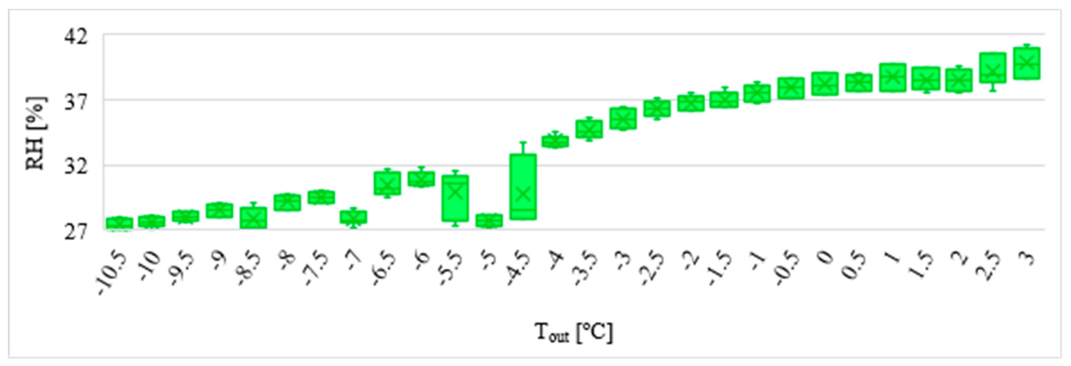
Figure 23 shows box plots illustrating the distribution of the humidity characteristic in groups defined by the outside temperature factor levels.
Table 13 contains the values of the Least Significant Difference LSD and test statistic W for the humidity characteristic, carried out according to the Tukey method in groups matching the levels of −10.5, −10, −9.5, −9, −8.5, −8, −7.5, −7, −6.5, −6, −5.5, −5, −4.5, −4, −3.5, −3, −2.5, −2, −1.5, −1, −0.5, 0, 0.5, 1, 1.5, 2, 2.5, and 3 °C of the outside temperature factor.
The tests of multiple comparisons carried out using the Tukey method for the humidity characteristic in groups defined by the outside temperature showed that the highest average humidity value should be expected for the outside temperature of 3 °C, and the lowest for the outside temperature of −10.5 °C.
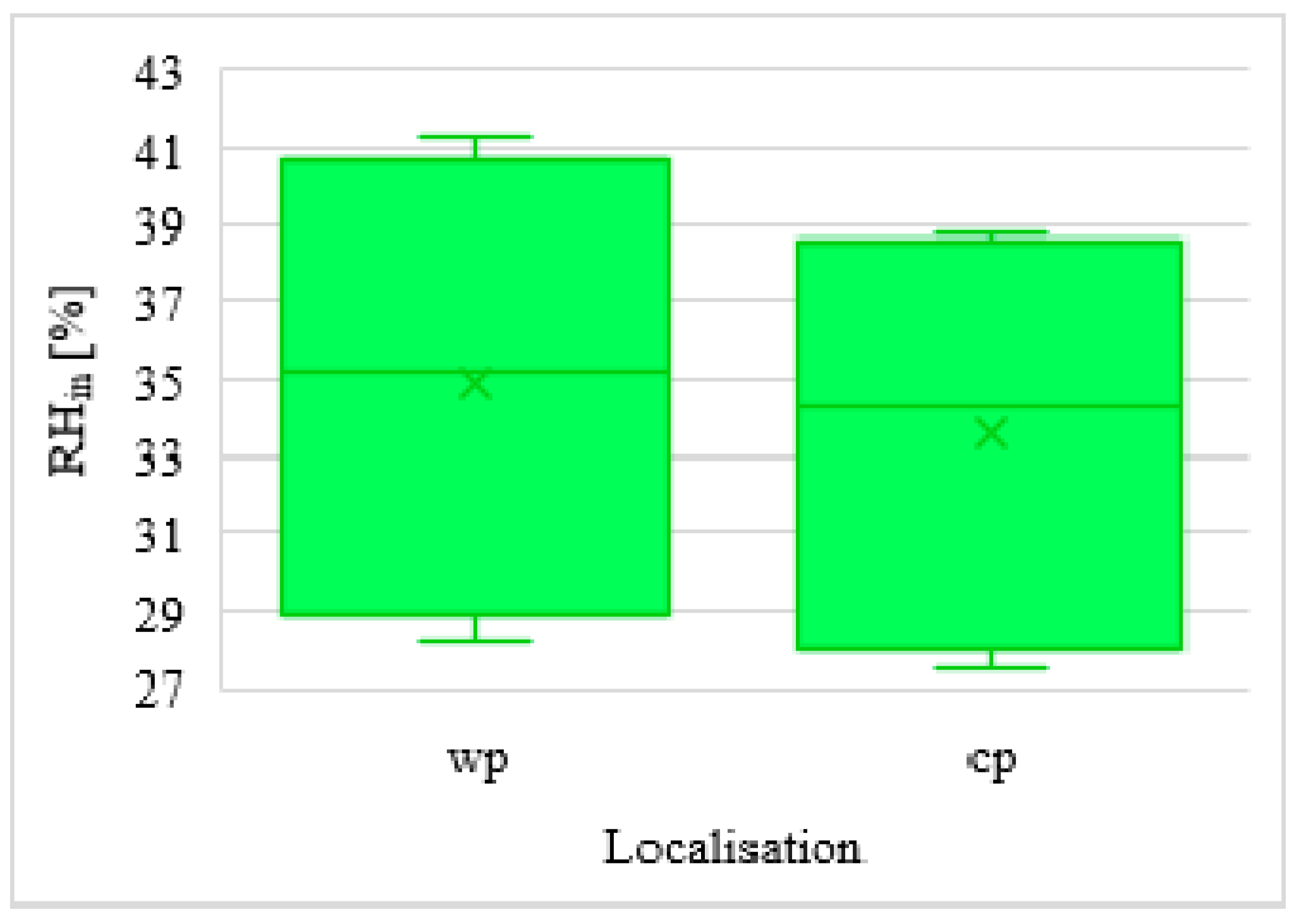
Figure 24 shows box plots illustrating the distribution of the humidity characteristic in groups defined by the location factor levels.
Table 14 contains the calculation results for the humidity characteristic, carried out according to the Tukey method in groups matching the workplace and central point levels of the location factor.
Table 14 shows that the average values of the humidity characteristic in the group defined by the workplace location were significantly higher than those corresponding to the central point location.
4. Conclusions
The interior microclimate is extremely important for the health and well-being of people staying in rooms. Sick building syndrome is a current problem that many building administrators and users must cope with, and most often results from an insufficient air exchange, occurring as a consequence of the excessive sealing of buildings. By and large, a great majority of existing buildings are ventilated naturally. Thermal modernization works are usually limited to the thermal insulation of building cladding and providing airtight window joinery. In most cases, there is no possibility of installing mechanical ventilation systems. In these cases, decentralized façade units may be the right solution for occupants to improve the indoor microclimate. Completed analysis of the patented solution has proven that, in spite of the lack of heat recovery exchanger and air heater, the unit does not reduce the inside air temperature below the comfort level while replacing used air with fresh air. Throughout the period of measurements, temperature values ranged within 20–22 °C. Moreover, the PMV value calculated on the basis of measurements showed that in the workplace, category B was maintained in the area of the head, abdomen, and feet, and the central point of the room was in category C at the end of the cycle (2 min). In the long cycle (10 min), it belonged to category C for almost the entire duration of the airflow (at all parts of the body). However, it should be mentioned that there is a risk of a local sensation of discomfort (draught) in the case where a user stands in the axis of the air stream and the air supply/exhaust cycle is long. In this case, the DR index at a distance of 70 cm from the supply/exhaust grate at the level of abdomen may be as high as 64%. It is recommended to use heat recovery from exhaust air and possibly an electric heater to warm up the air in order to eliminate the risk of negative air movement impact and the sensation of discomfort. Further studies will focus on the search for an optimal way to recover heat for decentralized ventilation units.
Air humidity analysis has proven that the value of this parameter value was too low and ranged within 27 to 43%. This indicates the need to find a way to humidify air in decentralized façade units.
The analyses of both temperature and humidity have proven that the values of inside air temperature and humidity are not affected by the temperature and humidity of outside air. In this case, it is important that negative pressure generated during the exhaust cycle induces an inflow of warm and dry air from an adjacent room.
The impact of using the decentralized façade unit on inside air parameters was analyzed for each of the three durations of air supply/exhaust cycle (2 min, 4 min, 10 min). In each of these cases, no temperature drop in the room was observed, and the air humidity was too low. Research results obtained during the experiment were evaluated from the statistical point of view. Completed statistical analysis proved that the average temperature values did not differ significantly for the outside temperature factor. On the other hand, in the case of the air supply/exhaust cycle duration setting, the average inside temperature was the highest for the shortest cycle and the lowest for the longest cycle.
In conclusion, it is necessary to carry out further tests of the decentralized façade units that would be used as an efficient way to improve the interior microclimate. However, it is necessary to find methods for heat recovery and air humidification.
5. Patents
The article presents the test results of patent-protected equipment: Zender-Świercz E., Piotrowski J. Room ventilation unit (2017). Patent no. PL 228624 B1.
Funding
This research was funded by the program of the Minister of Science and Higher Education under the name: “Regional Initiative of Excellence” in 2019–2022 project number 025/RID/2018/19, financing amount PLN 12,000,000.
Conflicts of Interest
The author declares no conflict of interest.
References
- Apte, M.G.; Fisk, W.J.; Daisey, J.M. Association between indoor CO2 concentration and sick building syndrome symptoms in U.S. office buildings:an analysis of the 1994—1996 BASE study data. Indoor Air 2000, 10, 246–257. [Google Scholar] [CrossRef] [PubMed] [Green Version]
- Apte, M.G.; Fisk, W.J.; Daisey, J.M. Indoor carbon dioxide concentrations and SBS in office workers. Proc. Healthy Build. 2000, 1, 133–138. [Google Scholar]
- Daisey, J.M.; Angell, W.J.; Apte, M. Indoor air quality, ventilation and health symptoms in schools: An analysis of existing information. Indoor Air 2003, 13, 53–64. [Google Scholar] [CrossRef] [PubMed]
- Haverinen-Shaughnessy, U.; Moschandreas, D.J.; Shaughnessy, R.J. Association between substandard classroom ventilation rates and students academic achievement. Indoor Air 2011, 21, 121–131. [Google Scholar] [CrossRef] [PubMed]
- Huttunen, K. Indoor Air Pollution. In Clinical Handbook of Air Pollution—Retated Diseases; Capello, F., Gaddi, A.V., Eds.; Springer: Modena, Italy, 2018; pp. 107–114. [Google Scholar] [CrossRef]
- Mendell, M.J.; Heath, G.A. Do indoor pollutants and thermal conditions in school influence student performance? A critical review of the literature. Indoor Air 2005, 15, 27–52. [Google Scholar] [CrossRef] [PubMed]
- Seppanen, O.A.; Fisk, W.J. Effects of temperature and outdoor air supply rate on the performance of call center operators in the tropics. Indoor Air 2004, 7, 102–118. [Google Scholar] [CrossRef] [PubMed] [Green Version]
- Seppanen, O.A.; Fisk, W.J.; Mendel, M.J. Association of ventilation rates and CO2 concentrations with health and other responses in commercial and industrial buildings. Indoor Air 1999, 9, 226–252. [Google Scholar] [CrossRef]
- Sowa, J. Jakość powietrza we wnętrzach jako istoty element pływający na komfort pracy. Cyrkulacje 2017, 37, 32–33. [Google Scholar]
- Telejko, M.; Zender-Świercz, E. An attempt to improve air quality in primary schools. 10th International Conference. Environ. Eng. 2017. [Google Scholar] [CrossRef]
- Zender-Świercz, E. Improving the indoor air quality using the Indyvidual Air Supply System. Int. J. Environ. Sci. Technol. 2018, 15, 689–696. [Google Scholar] [CrossRef] [Green Version]
- Zender-Świercz, E.; Telejko, M. The impact of insulation building on the work of ventilation. Procedia Eng. 2016, 161, 1731–1737. [Google Scholar] [CrossRef] [Green Version]
- Górny, R.L. Submikronowe Cząstki Grzybów i Bakterii—Nowe Zagrożenie Środowiska Wnętrz; Wydawnictwa Politechniki Warszawskiej: Warsaw, Poland, 2005; pp. 25–40. [Google Scholar]
- Fisk, W.J.; Mirer, A.G.; Mendell, M.J. Quantitative relationship of sick building syndrome symptoms with ventilation rates. Indoor Air 2009, 19, 159–165. [Google Scholar] [CrossRef] [PubMed] [Green Version]
- Muchič, S.; Butala, V. The influence of indoor environment in office building on their occupants: Expected—Unexpected. Build. Environ. 2004, 39, 289–296. [Google Scholar] [CrossRef]
- Runeson, R.; Wahlstedt, K.; Wieslander, G.; Norbäck, D. Personal and psychosocial factors and symptoms compatible with sick building syndrome in the Swedish workforce. Indoor Air 2006, 16, 445–453. [Google Scholar] [CrossRef] [PubMed]
- Brasche, S.; Bullinger, M.; Morfeld, M.; Gebhardt, H.J.; Bischof, W. Why do Women Suffer from Sick Building Syndrome more often than Men?—Subjective Higher Sensitivity versus Objective Causes. Indoor Air 2001, 11, 217–222. [Google Scholar] [CrossRef] [PubMed] [Green Version]
- Karjalainen, S. Gender differences in thermal comfort and use of thermostats in everyday thermal environments. Build. Environ. 2007, 42, 1594–1603. [Google Scholar] [CrossRef]
- Karjalainen, S. Thermal comfort and gender: A literature review. Indoor Air 2012, 22, 96–109. [Google Scholar] [CrossRef]
- Winarti, M.; Basuki, B.; Hamid, A. Air movement, gender and risk of sick building headache among employees in a Jakarta office. Med. J. Indones. 2003, 12, 171–177. [Google Scholar] [CrossRef]
- Lan, L.; Wargocki, P.; Lian, Z. Quantitative measurement of productivity loss due to thermal discomfort. Energy Build. 2011, 43, 1057–1062. [Google Scholar] [CrossRef]
- Klavina, A.; Proskurina, J.; Rodins, V.; Martinsone, I. Carbon dioxide as indoor air quality indicator in renovated schools in Latvia. In Proceedings of the Indoor Air 2016 The 14th International Conference of Indoor Air Quality and Climate, Ghent, Belgium, 3–8 July 2016. [Google Scholar]
- Roelofsen, P. The impact of office environments on employee performance:the design of the workplace as strategy for productivity enhancement. J. Facil. Manag. 2002, 1, 247–264. [Google Scholar] [CrossRef]
- Johnson, D.L.; Lynch, R.A.; Floyd, E.L.; Wang, J.; Bartels, J.N. Indoor air quality in classrooms: Environmental measures and effective ventilation rate modeling in urban elementary schools. Build. Environ. 2018. [Google Scholar] [CrossRef]
- Vimalanathan, K.; Babu, T.R. The effect of indoor office environment on the work performance, health and welbeing of office workers. J. Environ. Health Sci. 2014, 12, 113. [Google Scholar] [CrossRef] [PubMed] [Green Version]
- Mijakowski, M. Wilgotność Powietrza w Relacjach Człowiek, Środowisko Wewnętrzne, Architektura; Wydawnictwa Politechniki Warszawskiej: Warsaw, Poland, 2005; pp. 105–121. [Google Scholar]
- Polish Committee for Standardization. PN EN 13788:2013-05 Hygrothermal Performance of Building Components and Building Elements—Internal Surface Temperature to Avoid Critical Surface Humidity and Interstitial Condensation—Calculation Methods; Polish Committee for Standardization: Warszawa, Poland, 2016. [Google Scholar]
- Pogorzelski, J.A. Zagadnienia Cieplno—Wilgotnościowe Przegród Budowlanych; Budownictwo ogólne, P., Ed.; Arkady: Warsaw, Poland, 2005. [Google Scholar]
- Kisilewicz, T. O związkach między szczelnością budynków, a mikroklimatem, komfortem wewnętrznym i zużyciem energii w budynkach niskoenergetycznych. Napędy Sterow. 2014, 12, 94–97. [Google Scholar]
- Lazovic, I.; Stevanović, Z.M.; Jovašević-Stojanović, M.; Živković, M.M.; Banjac, M. Impact of CO2 concentration on indoor air quality and correlation with relative humidity and indoor air temperature in school building in Serbia. Therm. Sci. 2015, 20, 173. [Google Scholar] [CrossRef]
- Nomura, M.; Hiyama, K. A review: Natural ventilation performance of office buildings in Japan. Renew. Sustain. Energy Rev. 2017, 74, 746–754. [Google Scholar] [CrossRef]
- Fanger, P.O.; Popiołek, Z.; Wargocki, P. Środowisko Wewnętrzne. Wpływ na Zdrowie, Komfort i Wydajność Pracy; Wydawnictwo Politechniki Śląskiej: Gliwice, Poland, 2003. [Google Scholar]
- Fanger, P.O.; Melikov, A.K.; Hanzawa, H.; Ring, J. Air turbulence and sensation of draught. Energy Build. 1988, 12, 21–39. [Google Scholar] [CrossRef]
- Toftum, J.; Zhou, G.; Melikov, A.K. Effect of Airflow Direction on Human Perception of Draught. Available online: https://pdfs.semanticscholar.org/3a9b/c78141659022d3e207879b65a240c9820ea4.pdf (accessed on 20 May 2020).
- Coydon, F.; Herkel, S.; Kuber, T.; Pfafferott, J.; Himmelsbach, S. Energy performance of façade integrated decentralised ventilation systems. Energy Build. 2015, 107, 172–180. [Google Scholar] [CrossRef]
- Merzkirch, A.; Mass, S.; Scholzen, F.; Waldmann, D. Primary energy used in centralised and decentralised ventilation systems measured in field tests in residential buildings. Int. J. Vent. 2019, 18, 19–27. [Google Scholar] [CrossRef]
- Dermentzis, G.; Ochs, F.; Siegele, D.; Feist, W. Renovation with an innovative compact heating and ventilation system integrated into the façade—An in-situ monitoring case study. Energy Build. 2018, 165, 451–463. [Google Scholar] [CrossRef]
- Gruner, M.; Haase, M. The Potential of Façade-Integrated Ventilation Systems in Nordic Climate. In Advanced Decentralised Ventilation Systems as Sustainable Alternative to Conventional Systems; NTNU: Trondheim, Norway, 2012. [Google Scholar]
- Energy Performance of Buildings. Ventilation for Buildings. Indoor Environmental Input Parameters for Design and Assessment of Energy Performance of Buildings Addressing Indoor Air Quality, Thermal Environment, Lighting and Acoustics. Module M1-6; PN EN 16798-1:2019-06; Polish Committee for Standardization: Warsaw, Poland, 2019. [Google Scholar]
- Indoor Environmental Input Parameters for Design and Assessment of Energy Performance of Buildings Addressing Indoor Air Quality, Thermal Environment, Lighting and Acoustics; PN EN 15251: 2012; Polish Committee for Standardization: Warsaw, Poland, 2012.
- Mikola, A.; Simson, R.; Kurnitski, J. The Impact of Air Pressure Conditions on the Performance of Single Room Ventilation Units in Multi-Story Buildings. Energies 2019, 12, 2633. [Google Scholar] [CrossRef] [Green Version]
- Zemitis, J.; Bogdanovics, R. Heat recovery efficiency of local decentralized ventilation devices. Mag. Civ. Eng. 2020, 94, 120–128. [Google Scholar] [CrossRef]
- Ergonomics of the Thermal Environment—Analytical Determination and Interpretation of Thermal Comfort Using Calculation of the PMV and PPD Indices and Local Thermal Comfort Criteria; PN EN 7730; Polish Committee for Standardization: Warsaw, Poland, 2006.
- Catalina, T.; Istrate, M.A.; Damian, A.; Vartires, A.; Dicu, T.; Cucoş, A. Indoor air quality assessment in a classroom using a heat recovery ventilation unit. Rom. J. Phys. 2019, 64, 9–10. [Google Scholar]
- Ventilation for Acceptable Indoor Air Quality; ASHRAE-ANSI-ASHRAE Standard 62.1-2016; ASHRAE: Atlanta, GA, USA, 2016.
Figure 1.
Layout of meters and the decentralized façade unit in the analyzed room.

Figure 2.
Wall-mounted decentralized façade ventilation unit.

Figure 3.
Indoor air quality monitor.

Figure 4.
Average air temperature values at two locations in the room: (a) workplace, (b) central point of the room; Tint—inside temperature, °C; t—time, h:min.
Figure 4.
Average air temperature values at two locations in the room: (a) workplace, (b) central point of the room; Tint—inside temperature, °C; t—time, h:min.

Figure 5.
The dependence between the average outside air temperature and average value of the parameter inside the room: (a) setting: 2 min, (b) setting: 4 min, (c) setting: 10 min; T—temperature, °C; t—time, h:min.
Figure 5.
The dependence between the average outside air temperature and average value of the parameter inside the room: (a) setting: 2 min, (b) setting: 4 min, (c) setting: 10 min; T—temperature, °C; t—time, h:min.


Figure 6.
The dependence between inside air temperature and outside air temperature; Tint—inside temperature, °C; Tout—outside temperature, °C.
Figure 6.
The dependence between inside air temperature and outside air temperature; Tint—inside temperature, °C; Tout—outside temperature, °C.

Figure 7.
The course of changes in the indoor air temperature during the 10-min supply/exhaust cycle. (a) workplace; (b) central point.
Figure 7.
The course of changes in the indoor air temperature during the 10-min supply/exhaust cycle. (a) workplace; (b) central point.

Figure 8.
The course of changes in the indoor air temperature during the 2-min supply/exhaust cycle. (a) workplace; (b) central point.
Figure 8.
The course of changes in the indoor air temperature during the 2-min supply/exhaust cycle. (a) workplace; (b) central point.

Figure 9.
The course of changes in the indoor air temperature for an example day. (a) workplace; (b) central point.
Figure 9.
The course of changes in the indoor air temperature for an example day. (a) workplace; (b) central point.

Figure 10.
Average air humidity values at two locations in the room: (a) workplace, (b) central point of the room; RH—humidity, %; t—time, h:min.
Figure 10.
Average air humidity values at two locations in the room: (a) workplace, (b) central point of the room; RH—humidity, %; t—time, h:min.

Figure 11.
The dependence between the average outside air humidity and average value of the parameter inside the room: (a) setting: 2 min, (b) setting: 4 min, (c) setting: 10 min; RH—humidity, %; t—time, h:min.
Figure 11.
The dependence between the average outside air humidity and average value of the parameter inside the room: (a) setting: 2 min, (b) setting: 4 min, (c) setting: 10 min; RH—humidity, %; t—time, h:min.

Figure 12.
The relationship of the relative humidity of indoor air on the outdoor air temperature.

Figure 13.
The course of the air velocity and air volume changes in the supply/exhaust grate during the supply and exhaust cycle.
Figure 13.
The course of the air velocity and air volume changes in the supply/exhaust grate during the supply and exhaust cycle.

Figure 14.
The course of changes in the predicted mean vote (PMV) indicator during the 2-min cycle airflow. (a) workplace, (b) central point of the room, (c) 70 cm from the air supply grate; wp: workplace; cp: central point.
Figure 14.
The course of changes in the predicted mean vote (PMV) indicator during the 2-min cycle airflow. (a) workplace, (b) central point of the room, (c) 70 cm from the air supply grate; wp: workplace; cp: central point.

Figure 15.
The course of changes in the PMV indicator during the 10-min cycle airflow. (a) Workplace, (b) central point of the room, (c) 70 cm from the air supply grate; wp: workplace; cp: central point.
Figure 15.
The course of changes in the PMV indicator during the 10-min cycle airflow. (a) Workplace, (b) central point of the room, (c) 70 cm from the air supply grate; wp: workplace; cp: central point.

Figure 16.
The course of changes in the concentration of carbon dioxide. Blue and purple colors are the 2 min cycle; yellow and green colors are the 10 min cycle; wp: workplace; cp: central.
Figure 16.
The course of changes in the concentration of carbon dioxide. Blue and purple colors are the 2 min cycle; yellow and green colors are the 10 min cycle; wp: workplace; cp: central.

Figure 17.
Box plots illustrating the distribution of the temperature characteristic in groups defined by pairs of factors: setting and location; Tint—temperature, °C; wp: workplace; cp: central point.
Figure 17.
Box plots illustrating the distribution of the temperature characteristic in groups defined by pairs of factors: setting and location; Tint—temperature, °C; wp: workplace; cp: central point.

Figure 18.
Box plots illustrating the distribution of the temperature characteristic in groups defined by setting factor levels; Tint—temperature, °C.
Figure 18.
Box plots illustrating the distribution of the temperature characteristic in groups defined by setting factor levels; Tint—temperature, °C.

Figure 19.
Box plots illustrating the distribution of the temperature characteristic in groups defined by location factor levels; Tint—temperature, °C; wp: workplace; cp: central point.
Figure 19.
Box plots illustrating the distribution of the temperature characteristic in groups defined by location factor levels; Tint—temperature, °C; wp: workplace; cp: central point.

Figure 20.
Box plots illustrating the distribution of the temperature characteristic in groups defined by pairs of factors: setting and outside temperature; Tint—inside temperature, °C; Tout—outside temperature, °C.
Figure 20.
Box plots illustrating the distribution of the temperature characteristic in groups defined by pairs of factors: setting and outside temperature; Tint—inside temperature, °C; Tout—outside temperature, °C.

Figure 21.
Box plots illustrating the distribution of the temperature characteristic in groups defined by outside temperature factor levels; Tint—temperature, °C; Tout—outside temperature, °C
Figure 21.
Box plots illustrating the distribution of the temperature characteristic in groups defined by outside temperature factor levels; Tint—temperature, °C; Tout—outside temperature, °C

Figure 22.
Box plots illustrating the distribution of the humidity characteristic in groups defined by pairs of factors: outside temperature and location; RHin—humidity, %; Tout—outside temperature, °C; wp: workplace; cp: central point.
Figure 22.
Box plots illustrating the distribution of the humidity characteristic in groups defined by pairs of factors: outside temperature and location; RHin—humidity, %; Tout—outside temperature, °C; wp: workplace; cp: central point.

Figure 23.
Box plots illustrating the distribution of the humidity characteristic in groups defined by outside temperature factor levels; RHin—humidity, %; Tout—outside temperature, °C.
Figure 23.
Box plots illustrating the distribution of the humidity characteristic in groups defined by outside temperature factor levels; RHin—humidity, %; Tout—outside temperature, °C.

Figure 24.
Box plots illustrating the distribution of the humidity characteristic in groups defined by the location factor levels; RHin—humidity, %; wp: workplace; cp: central point.
Figure 24.
Box plots illustrating the distribution of the humidity characteristic in groups defined by the location factor levels; RHin—humidity, %; wp: workplace; cp: central point.


Table 1.
Measurement ranges and resolution of indications. Indoor air quality monitor.
| Parameter | Measurement Range | Resolution of Indications | Unit | Accuracy |
|---|---|---|---|---|
| Temperature | 10–45 | 0.1 | °C | ±0.5 |
| Humidity | 0–100 | 0.1 | % | ±2 |
| Carbon dioxide concentration | 0–5000 | 1 | ppm | ±(20 + 3% of meas. value) |
Table 2.
Microclimate meter specifications.
| Parameter | Measurement Range | Resolution of Indications | Unit | Accuracy |
|---|---|---|---|---|
| Air velocity | 0–5 | 0.01 | m/s | ±0.05 + 0.05 × Va for 0–1 m/s ±5% for 1–5 m/s |
| Radiant temperature | −20–50 | 0.01 | °C | ±0.4 °C |
Table 3.
Weather station specifications.
| Parameter | Measurement Range | Resolution of Indications | Unit | Accuracy |
|---|---|---|---|---|
| Temperature | −40–65 | 0.1 | °C | 0.5 |
| Humidity | 1–100 | 1 | % | 3% RH; 4% over 90% |
Table 4.
The specifications of balometer station.
| Parameter | Measurement Range | Resolution of Indications | Unit | Accuracy |
|---|---|---|---|---|
| Volumetric flow rate | 42–4250 | 1 | m3/h | ±3% read out value ± 12 m³/h > 85 m³/h |
| Air speed | 0.125–12.5 | 0.01 | m/s | ±3% read out value ± 0.04 m/s > 0.25 m/s |
| Temperature | −40–121 | 0.1 | °C | ±0.3% °C |
| Humidity | 5–95 | 0.1 | % | ±3% RH |
Table 5.
Analysis of variance for the temperature characteristic.
| Variability | Degrees of Freedom | Sum of the Squares | Mean Square | Value F | Value p |
|---|---|---|---|---|---|
| Intergroup | 5 | 7.7 | 1.5 | 81.3 | <0.0001 |
| Intragroup | 30 | 0.6 | 0.02 | ||
| Total | 35 | 8.2 |
Table 6.
The Tukey multiple comparison method tests for the temperature characteristic in groups defined on the basis of the setting factor levels. No. of Average Values: 3. Least significant difference: 0.12.
Table 6.
The Tukey multiple comparison method tests for the temperature characteristic in groups defined on the basis of the setting factor levels. No. of Average Values: 3. Least significant difference: 0.12.
| Tukey Grouping | Average | N | Setting |
|---|---|---|---|
| A | 21.5 | 12 | 2 |
| B | 21.1 | 12 | 4 |
| C | 20.9 | 12 | 10 |
Table 7.
Simultaneous 95-percent confidence intervals obtained using the Tukey method for the difference in avg. values of temperature in groups matching setting levels.
Table 7.
Simultaneous 95-percent confidence intervals obtained using the Tukey method for the difference in avg. values of temperature in groups matching setting levels.
| Comparison | Difference between Avg. Values | Simultaneous 95-Percent Confidence Intervals | |
|---|---|---|---|
| Lower Limit | Upper Limit | ||
| 2–4 | 0.5 | 0.3 | 0.6 |
| 4–2 | −0.5 | −0.6 | −0.3 |
| 2–10 | 0.6 | 0.5 | 0.8 |
| 10–2 | −0.6 | −0.8 | −0.5 |
| 4–10 | 0.2 | 0.002 | 0.3 |
| 10–4 | −0.2 | −0.3 | −0.002 |
Table 8.
The Tukey multiple comparison method tests for the temperature characteristic in groups defined on the basis of the location factor levels. No. of Average Values: 2. Least significant difference: 0.096.
Table 8.
The Tukey multiple comparison method tests for the temperature characteristic in groups defined on the basis of the location factor levels. No. of Average Values: 2. Least significant difference: 0.096.
| Tukey Grouping | Average | N | Setting |
|---|---|---|---|
| A | 21.5 | 18 | wp |
| B | 20.8 | 18 | cp |
Table 9.
Simultaneous 95-percent confidence intervals obtained using the Tukey method for difference in avg. values of temperature in groups matching location levels.
Table 9.
Simultaneous 95-percent confidence intervals obtained using the Tukey method for difference in avg. values of temperature in groups matching location levels.
| Comparison | Difference between Avg. Values | Simultaneous 95-Percent Confidence Intervals | |
|---|---|---|---|
| Lower Limit | Upper Limit | ||
| wp–cp | 0.7 | 0.5 | 0.9 |
| cp–wp | −0.7 | −0.9 | −0.5 |
Table 10.
Analysis of variance for the temperature characteristic.
| Variability | Degrees of Freedom | Sum of the Squares | Mean Square | Value F | Value p |
|---|---|---|---|---|---|
| Intergroup | 5 | 2.9 | 0.6 | 3.3 | 0.025 |
| Intragroup | 30 | 5.3 | 0.2 | ||
| Total | 35 | 8.2 |
Table 11.
The Tukey multiple comparison method tests for the temperature characteristic in groups defined on the basis of the outside temperature factor levels. No. of Average Values: 2. Least significant difference: 0.3.
Table 11.
The Tukey multiple comparison method tests for the temperature characteristic in groups defined on the basis of the outside temperature factor levels. No. of Average Values: 2. Least significant difference: 0.3.
| Tukey Grouping * | Average | N | Setting |
|---|---|---|---|
| A | 21.22 | 18 | −7 |
| A | 21.12 | 18 | −3 |
* Average values marked with the same letter do not differ significantly.
Table 12.
Analysis of variance for the humidity characteristic.
| Variability | Degrees of Freedom | Sum of the Squares | Mean Square | Value F | Value p |
|---|---|---|---|---|---|
| Intergroup | 55 | 3488.2 | 63.4 | 126.9 | <0.0001 |
| Intragroup | 112 | 56.0 | 0.5 | ||
| Total | 167 | 3544.2 |
Table 13.
The Tukey multiple comparison method tests for the humidity characteristic in groups defined on the basis of the outside temperature factor levels.
Table 13.
The Tukey multiple comparison method tests for the humidity characteristic in groups defined on the basis of the outside temperature factor levels.
| No. of Average Values | 28 |
| Least Significant Difference | 0.15 |
| Test Statistic W | 1.18 |
Table 14.
The Tukey multiple comparison method tests for the humidity characteristic in groups defined on the basis of the location factor levels. No. of Average Values: 2. Least significant difference: 0.08.
Table 14.
The Tukey multiple comparison method tests for the humidity characteristic in groups defined on the basis of the location factor levels. No. of Average Values: 2. Least significant difference: 0.08.
| Tukey Grouping | Average | N | Setting |
|---|---|---|---|
| A | 34.9 | 42 | wp |
| B | 33.6 | 42 | cp |
© 2020 by the author. Licensee MDPI, Basel, Switzerland. This article is an open access article distributed under the terms and conditions of the Creative Commons Attribution (CC BY) license (http://creativecommons.org/licenses/by/4.0/).
Share and Cite
MDPI and ACS Style
Zender-Świercz, E. Microclimate in Rooms Equipped with Decentralized Façade Ventilation Device. Atmosphere 2020, 11, 800. https://doi.org/10.3390/atmos11080800
AMA Style
Zender-Świercz E. Microclimate in Rooms Equipped with Decentralized Façade Ventilation Device. Atmosphere. 2020; 11(8):800. https://doi.org/10.3390/atmos11080800
Chicago/Turabian StyleZender-Świercz, Ewa. 2020. "Microclimate in Rooms Equipped with Decentralized Façade Ventilation Device" Atmosphere 11, no. 8: 800. https://doi.org/10.3390/atmos11080800
Note that from the first issue of 2016, this journal uses article numbers instead of page numbers. See further details here.