


Introduction
Autonomous phase-sensitive radio-echo sounder (ApRES) is a frequency-modulated continuous wave (FMCW) radar originally developed to measure the rate of melting at the base of Antarctic ice shelves (Brennan and others, Reference Brennan, Lok, Nicholls and Corr2014; Nicholls and others, Reference Nicholls2015). Its primary advantage over pRES, an earlier version of the system (Corr and others, Reference Corr, Jenkins, Nicholls and Doake2002), is that it can operate autonomously for a year or more in an Antarctic setting, while sampling at relatively high temporal frequency (hourly, for example). ApRES is deployed at the ice surface and it provides a Lagrangian measurement of the ice column beneath; typical analysis involves identification of temporal evolution of near-surface processes (e.g. firn compaction), internal processes (e.g. vertical strain rate), and processes at the ice base (e.g. melt rate) by inspecting the changes in vertical position of internal and basal reflectors.
ApRES and pRES have been successfully employed in a number of applications including measuring ice velocities and strain rates of slow moving grounded ice (Gillet-Chaulet and others, Reference Gillet-Chaulet, Hindmarsh, Corr, King and Jenkins2011; Kingslake and others, Reference Kingslake2014, Reference Kingslake, Martín, Arthern, Corr and King2016), measuring the orientation of dipping internal reflectors using an ApRES array in multiple-input multiple-output imaging mode (Young and others, Reference Young2018), inference of ice fabric characteristics from polarimetric measurements (Brisbourne and others, Reference Brisbourne2019; Jordan and others, Reference Jordan, Schroeder, Elsworth and Siegfried2020) and detection of ice shelf dynamics and basal melting at tidal timescales (Jenkins and others, Reference Jenkins, Corr, Nicholls, Stewart and Doake2006; Vaňková and others, Reference Vaňková, Nicholls, Corr, Makinson and Brennan2020). The instrument is now being used to obtain time series in increasingly more diverse environments such as Greenland's glaciers both floating (Washam and others, Reference Washam, Nicholls, Münchow and Padman2019) and grounded; the latter studies have targeted processes such as changing englacial meltwater content (Kendrick and others, Reference Kendrick2018; Vaňková and others, Reference Vaňková2018) and seasonal evolution of vertical strain rates (Young and others, Reference Young2019).
This observational technique offers exciting new opportunities, but at times the interpretation of the data presents significant challenges, in particular when the data come from deployments in glaciologically complicated environments. Some complications can also be caused by poor data quality from sites with potentially high surface glacial melt where signal strength may vary significantly on daily timescales. In this paper, we investigate the impact of different instrument settings when ApRES data have been partly corrupted as a result of receiver saturation due to excessive signal strength.
ApRES background
Here we briefly summarize the practical ApRES operation and pre-processing steps that are relevant to the following discussion. Details can be found in Brennan and others (Reference Brennan, Lok, Nicholls and Corr2014) and Nicholls and others (Reference Nicholls2015).
ApRES is deployed on a glacier surface. The instrument transmits a sequence of chirps, each consisting of a tone whose frequency smoothly ramps from 200 to 400 MHz over a period of 1 s; the transmit power is nominally 100 mW. The received signal then passes through an amplifier, an adjustable attenuator, another amplifier and finally it is frequency-deramped by mixing with a copy of the transmitted signal. An active filter (AF) then preferentially enhances the higher frequencies with three selectable gain settings, called the AF gain. The signal is then digitized and stored. The analog-to-digital converter has a voltage range of 0–2.5 V. This means that if the deramped chirp exceeds these limits, a clipped (and therefore corrupted) version of the deramped signal is written to the data file. The adjustable attenuator and the AF gain settings are used to set the receiver sensitivity. The attenuation level can be set between 0 and 31.5 dB, with the higher values needed in the presence of strong near-surface reflectors. The options for the AF gain are −14, −4, and +6 dB. These settings are generally chosen after the ApRES has been installed on the glacier surface and a test chirp has been recorded. If this is not possible, up to four combinations of settings can be used, in which case, up to four sequences of chirps are sequentially transmitted and recorded for each observation. Subsequent post-processing steps are centered on spectral analysis, because each frequency (f d) contained in a deramped chirp of an FMCW radar sounder is related to a unique reflector range (R) via (Skolnik, Reference Skolnik2008; Brennan and others, Reference Brennan, Lok, Nicholls and Corr2014):

where B is the transmitted chirp's bandwidth, c is the speed of light in vacuum, ε r is the relative dielectric constant of ice, and T is the pulse duration. If a sequence of chirps is collected, a typical product of the post-processing is a time series of return amplitude at different ranges, and a time series of vertical displacements of different internal reflectors with respect to the instrument's antennas at the glacier surface.
Data and methods
In June 2017, an ApRES was deployed at Jakobshavn Isbræ in West Greenland at site J1Y17, located ~15 km from the calving front. Because it was known that operational conditions would not allow the instrument settings to be configured at the site, three different attenuator values were used in the ApRES configuration file: 15, 20 and 30 dB. The AF gain was kept at the −4 dB level for each of the three settings. The data were then processed separately for each configuration setting following Nicholls and others (Reference Nicholls2015), and vertical displacement time series of internal reflectors were constructed by differencing the phase of subsequent measurements.
We also revisit ApRES data collected at Helheim Glacier in Southeast Greenland in August 2016 and described in Vaňková and others (Reference Vaňková2018). A single attenuator setting of 20 dB was used at all Helheim sites with the AF gain kept at the −4 dB. These data have shown strong depth-dependent diurnal signals in the vertical displacement time series of the internal reflectors. The vertical structure of this diurnal signal was studied by constructing a composite diurnal variation of each depth level, a technique also used here.
Results
Figure 1 shows the return amplitude and vertical cumulative displacements from site J1Y17 for each of the three attenuator settings. The 30 dB attenuation produces a typical ApRES return amplitude profile where the amplitude quickly decays with range; there is little change through time inside the ice column, and a basal reflector can be distinguished at ~600 m range (Fig. 1a1). For the 20 dB attenuation, the recorded signal amplitude increases, as expected. In addition, there is a temporal change in the record and periods of enhanced return are introduced (Fig. 1b1). This enhanced return temporarily obscures the visibility of the basal reflector, which is otherwise well distinguishable outside this time period. Finally, the 15 dB attenuation results in a higher recorded signal amplitude throughout the record, and the basal reflector is no longer detectable (Fig. 1c1). The vertical displacement time series (Fig. 1, second row) for the 30 dB attenuation show a diurnal signal in the upper 400 m of the ice column, but this signal is absent at greater ranges (Fig. 1a2). The time series generated for the 20 dB attenuation setting has this diurnal signal present at all ranges (Fig. 1b2). For the lowest, 15 dB, attenuation this diurnal signal appears to be increasing with range (Fig. 1c2).
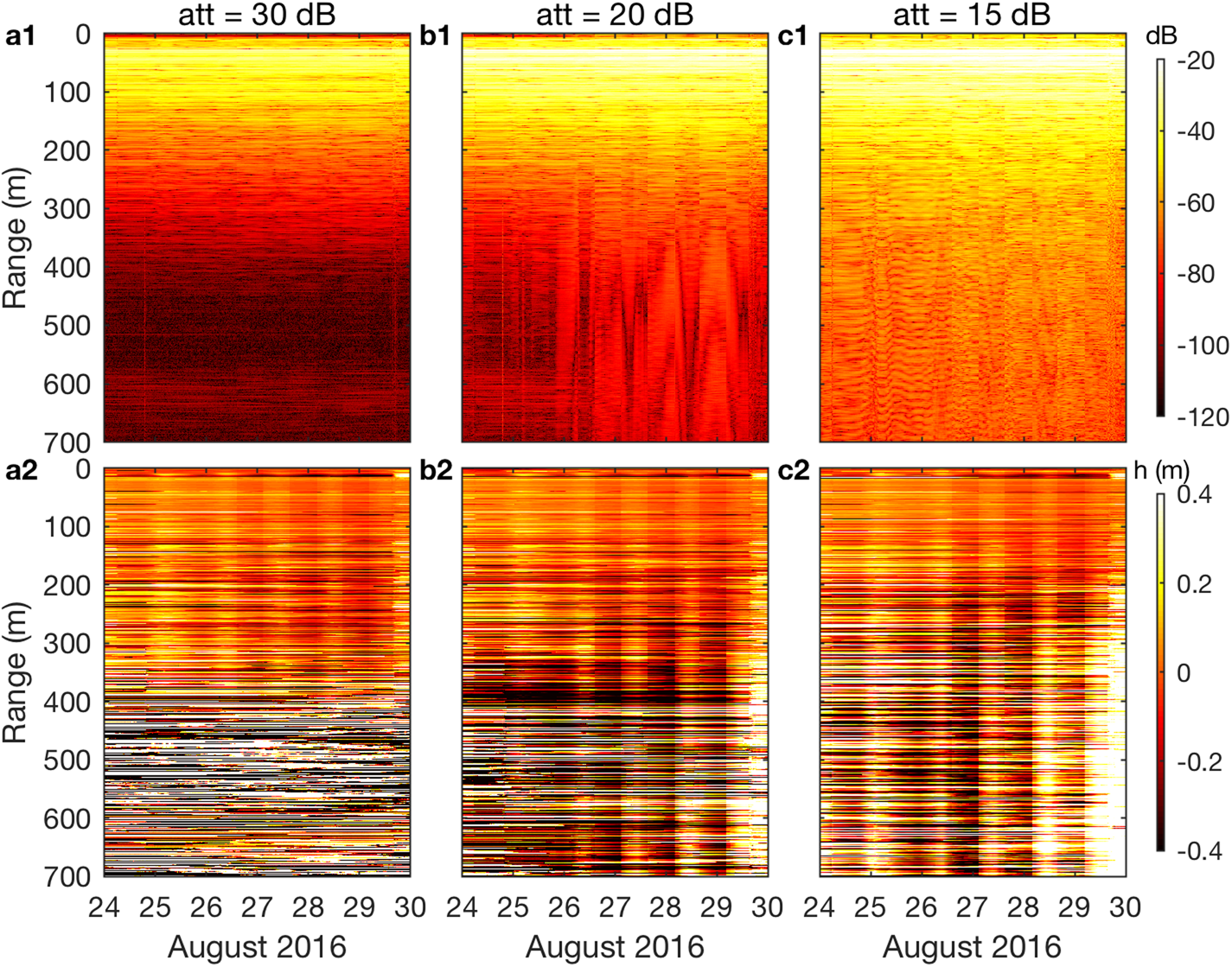
Fig. 1. ApRES return signal from site J1Y17. The full deramped chirp, generated by a transmitted chirp in the 200–400 MHz frequency band has been processed for the three attenuation settings: (a) 30 dB, (b) 20 dB and (c) 15 dB. Return amplitude is plotted in the first row and the detrended cumulative vertical displacement, h, in the second row.
To investigate the differences between the three attenuator settings, we turn to the original deramped chirp prior to any post processing. The deramped chirp envelope, the maximum value a deramped chirp has taken for each transmitted frequency through the observation period, is plotted in Figure 2a. It shows that the deramped chirp has been clipped at some point of the record for all the attenuation settings. For the 15 dB attenuation setting, the full first half of the deramped chirp has been corrupted.
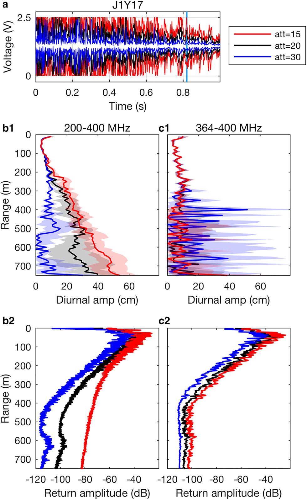
Fig. 2. Observations from site J1Y17. (a) Deramped chirp envelope for the entire observation period. The light blue line indicates the time of 0.82 s, past which the signal is free from clipping for all three attenuator settings at all times. (b1) Vertical profile of diurnal amplitude of the apparent cumulative vertical displacement (one std dev. is shaded) for the full deramped chirp (200–400 MHz band) and (c1) for the 0.82–1 s deramped chirp subinterval (364–400 MHz band). (b2) Vertical profile of the time averaged return signal amplitude for the full deramped chirp and (c2) for the 0.82–1 s deramped chirp subinterval.
As Figure 2a shows, the deramped chirp amplitude decreases with time and there is a subinterval toward the end of the record during which no clipping occurred for any of the configuration settings. As any given subinterval of the deramped chirp contains all the required spectral information (except for the very lowest frequencies), we can select a portion of the deramped chirp uncorrupted by clipping and perform the usual processing steps. Each subinterval in the 1-s long deramped chirp has been generated by a corresponding frequency band of the transmitted chirp in line with the chirp ramp specifications. The consequence of shortening the subinterval, and thus reducing the bandwidth, is a lower vertical resolution and a lower signal-to-noise ratio (Brennan and others, Reference Brennan, Lok, Nicholls and Corr2014). For site J1Y17, clipping is avoided when processing is restricted to the subinterval between 0.82 and 1 s, which has been generated by the 364–400 MHz frequency band of the transmitted chirp.
Figures 2b1 and c1 compare differences in the strength of the diurnal signal in the vertical displacement for site J1Y17 between processing the full 1-s deramped chirp and a reduced portion of the deramped chirp in the subinterval between 0.82 and 1 s. These figures shows the amplitude of the diurnal signal composite as a function of range. While the diurnal signal increases with decreasing attenuator setting for the full deramped chirp, that is no longer the case for the reduced deramped chirp. In the upper 300 m the vertical structure of the diurnal signal is the same for all attenuation settings. The return amplitude (Figs 2b2 and c2) decreases linearly down to 300 m range for all settings and then it levels off at ~−100 dB for greater ranges, indicating that farther than 300 m the signal is dominated by noise. Accordingly, the diurnal signal in the vertical displacement is no longer distinguishable with any setting.
The comparison in Figure 2 demonstrates that the observed differences between the different attenuator settings, and in particular the appearance of a linear increase of diurnal amplitude with range in the cases of the lower attenuations, are caused by clipping artifacts. These clipping artifacts also appear to be responsible for increased return amplitude at greater ranges, which may result in obscuring internal reflectors and even the basal reflector (Figs 1c1 and 2b2).
Discussion
The character of clipping artifacts is a result of the introduction of square-wave-like features (e.g. Fig. 2a). When spectrally analyzed, these square waves appear as a sequence of harmonics. To illustrate the effects of clipping we consider the frequency content both of a deramped signal consisting of a pure sine wave, that is, the result of a single plane reflector at normal incidence, and of its clipped equivalent. $\hat{s}_N\lpar f \rpar$ in Eqn (2) represents the Fourier transform of both cases:
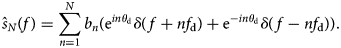
Setting N = 1 gives the unclipped signal, and setting N → ∞ and using an appropriate choice of coefficients b n, yields the square-wave version. In Eqn (2) f is the frequency, θ d = 2πf dt o is the phase of the fundamental frequency f d for a time shift t o, and δ is the delta function. From Eqn (2), it is clear that introduction of square-wave features will give rise to harmonics, which in the processed ApRES data will appear as equally-spaced reflectors through depth because of the linear relationship between f d and R in Eqn (1). When the actual reflector moves vertically, this will be expressed as both a change of frequency (from Eqn (1)) and a change of phase. The effect of changing frequency can be seen by substituting f d = f d + df d into Eqn (2). Because the nth harmonic of frequency nf d will have changed its frequency by ndf d, deeper reflectors will experience larger apparent displacement, the effect being linear. Similarly, the effect of changing phase of the fundamental frequency can be seen by substituting θ d = θ d + dθ d into Eqn (2). The phase of the nth harmonic will have shifted by ndθ d, again producing an apparent linearly depth-increasing displacement in the processed clipped data.
Synthetic example
To further illustrate how clipping causes depth-increasing artifacts in the ApRES vertical displacement time series, we construct the following synthetic examples (results shown in Fig. 3). We generate a synthetic deramped signal consisting of different frequencies between 25 and 500 Hz. To simulate a vertical diurnal motion, the phase of each single-frequency component is varied sinusoidally through time. The 1-s long signal is sampled at 40 kHz, as in the ApRES. The amplitude of the phase variation linearly increases between 100 and 300 Hz and then decreases linearly to zero between 300 and 500 Hz; below 100 Hz the phase is constant. Finally, Gaussian noise at the power levels of −160 dBW is added to the sum of the single-frequency signals to increase the realism of the simulation. Applying ApRES processing to this synthetic deramped signal results in a series of reflections, each corresponding to one frequency, consistent with Eqn (1) (Fig. 3a1). Because the phase of the internal reflectors is varied diurnally, there is a diurnal signal present in the cumulative vertical displacement time series. As prescribed, the diurnal signal first increases, and then decreases with range (Fig. 3a2). Below the deepest reflector, only Gaussian noise is present. Oscillations in the return amplitude may be visible depending on the noise level; however, those are window-dependent artifacts resulting from spectral leakage (Fig. 3, top row). In the next experiment, we clip the synthetic deramped signal whenever a voltage threshold is exceeded. Processing this clipped signal introduces harmonics and as a result artifacts appear in both return amplitude and vertical displacement time series (Fig. 3b). In the return amplitude the artifacts show as additional bright reflectors throughout depth (Fig. 3b1). The spacing between the artifacts depends on the position of the original reflector. Therefore, if the position of the reflector varies through time (here by changing the phase of the sinusoids that form the synthetic deramped signal), the spacing between the artifacts changes as well. This results in diurnal variations in the cumulative displacement time series whose amplitude increases with range (Fig. 3b2). Next we remove the time dependency and consider a constant unclipped and clipped synthetic voltage signal. In the return amplitude, the artifacts at depth remain the same as in the case of a time-independent clipped signal (Figs 3c1 and d1); harmonics are still present although they do not change in time. In the unclipped case there is no vertical motion (Fig. 3c2) where internal reflectors are present, and below the deepest reflector there is Gaussian noise as prescribed. In the clipped case, artifacts in the vertical displacement time series (Fig. 3d2) appear again, this time as well defined motionless layers. These examples show that clipping artifacts can overpower internal layers and lead to erroneous vertical velocity profile estimates.

Fig. 3. Synthetic deramped signal used to simulate internal reflector motion. The first row shows the return amplitude and the second row the cumulative vertical displacement, h. (a) The signal phase varies sinusoidally in time, (b) same as (a) but the signal is clipped, (c) the signal is constant in time and (d) same as (c) but the signal is clipped.
Helheim sites revisited
We now inspect the data recorded at Helheim in August 2016 and previously reported by Vaňková and others (Reference Vaňková2018). Two representative sites are H1Y16 and H3Y16. While for H1Y16 the diurnal signal was observed to increase with range throughout the ice column, for H3Y16 it was concentrated in the upper 300 m. Varying levels of clipping of the deramped chirp occurred throughout the record, but both sites experienced at least some clipping at some point in time. At H3Y16 clipping was intermittent and affected only a small number of points; however, at H1Y16 the signal was clipped at all times and the clipping level increased during the deployment.
As for J1Y17, the deramped chirp amplitude generally reduces with time, so processing its later segments generated by higher frequencies of the transmitted chirp can avoid clipping artifacts. Next we process different subintervals of the deramped chirp for the two sites and observe how this affects the vertical structure of the amplitude of the apparent diurnal motion. We consider deramped chirp subsets generated by the full chirp (200–400 MHz band), the second half of the chirp (300–400 MHz band) and the last quarter of the chirp (350–400 MHz band). Finally, we investigate clipping effects in a controlled way by enhancing the level of clipping artificially. This is done by removing the mean from the full deramped chirp, multiplying by a factor of 1.6, adding the mean back, and then clipping to the required 2.5 V voltage limits. Figure 4 shows the amplitude of the diurnal composite variation as a function of range for the different scenarios. For H3Y16 there is little change in the vertical structure of the diurnal amplitude generated from different subintervals of the deramped chirp, suggesting that a small amount of clipping is acceptable (Fig. 4, bottom row). However, for H1Y16 the clipping was sufficiently frequent to introduce artifacts at depth, producing a linearly increasing amplitude of diurnal variations with range for the case of the full deramped chirp (Fig. 4a1). When clipped portions of the signal are excluded, the amplitude of the final diurnal variations no longer shows a full-depth penetrating linearly increasing signal (Fig. 4b1). Instead the diurnal amplitude increases, reaches a maximum at ~200 m range, and then decreases. At ranges >350 m the diurnal signal is constant at both sites. Figure 4d illustrates the effect of forced clipping: the amplitude of the diurnal vertical displacement increases linearly with range, and the slope of the line is greater for stronger clipping.

Fig. 4. Vertical structure of the ApRES-derived diurnal variations at sites H1Y16 (top row) and H3Y16 (bottom row). All panels show diurnal depth-cumulative peak-to-peak displacement of each 10-m depth bin; shaded region lies within one std dev. from the mean (black line). Different subintervals of the deramped chirp are used: (a) full chirp (200–400 MHz band), (b) second half of the chirp (300–400 MHz band), (c) last quarter of the chirp (350–400 MHz band) and (d) full chirp (200–400 MHz band) multiplied by a factor of 1.6 and clipped to lie within the permitted voltage range.
Finally, in Figure 5 we use the unclipped portion of the data from site H3Y16 to show that clipping can introduce sufficient artifacts in the return amplitude to obscure the reflections from the glacier base as suggested by Figure 1. In the unclipped data the glacier base is visible at ~650 m depth (Fig. 5a). However, forced clipping introduces bright reflections throughout the ice column, making the basal reflection nearly indistinguishable (Fig. 5b).
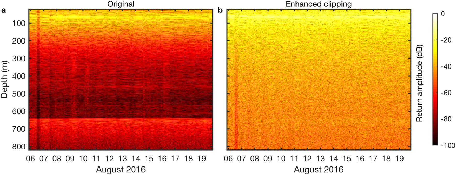
Fig. 5. Return amplitude at Helheim site H3Y16 (a) using the last quarter of the deramped chirp (350–400 MHz band) which avoids clipping, and (b) the full deramped chirp (200–400 MHz band) with clipping sufficiently enhanced to highlight how clipping obscures the bed return signal with artifacts.
Summary
Near-surface variation of meltwater content during ApRES deployments can substantially modulate the received signal strength on short timescales. Excessively strong signals may be clipped at some time during the observation period, even if the initial in situ test chirp produced a clean signal. Clipping introduces artifacts which manifest themselves in different ways. Artifacts in the return amplitude obscure returns from internal reflectors and the basal reflector, making it difficult to detect the thickness evolution of the ice and to correctly estimate vertical velocities. Additionally, if a near-surface internal reflector undergoes vertical position changes in time, an apparent linear increase of vertical displacement with depth will appear throughout the ice column. In general, any ApRES application that relies on the monitoring of internal layers will suffer artifacts if clipping occurs, because they overpower the real signal and may introduce artificial variability at depth. To avoid clipping-related problems, we recommend using higher attenuation settings for deployments in locations where changes in surface conditions are expected to occur. Alternatively, if the power and memory constraints allow, it is possible to use several attenuator and AF gain settings, one of which should be set at the lowest possible AF gain and the highest possible attenuation level.
Acknowledgements
We are grateful to the support provided from New York University Abu Dhabi through grant G1204, the NASA Jet Propulsion Laboratory Oceans Melting Greenland (OMG) program, NSF grants ARC-1304137, ANT-0424589, AGS-1338832 and PLR-1443190, grant NSF-NERC-PLR-1738934, and Heising-Simons Foundation under grant 2018-0769. This project has received funding from the European Union's Horizon 2020 research and innovation programme under the Marie Skłodowska-Curie grant agreement no. 790062. The ApRES data are too large to be freely stored at a public repository. Therefore, these data are archived at an institutional repository at the New York University's Environmental Fluid Dynamics Laboratory server, and they are freely available upon request to efdl@nyu.edu. We thank two anonymous reviewers for their constructive feedback.


 Open access