On the Failure of Classic Elasticity in Predicting Elastic Wave Propagation in Gyroid Lattices for Very Long Wavelengths


1
CNRS, MSME, Univ Paris Est Creteil, F-94010 Creteil, France
2
CNRS, MSME, Univ Gustave Eiffel, F-77447 Marne-la-Vallée, France
*
Author to whom correspondence should be addressed.
Symmetry 2020, 12(8), 1243; https://doi.org/10.3390/sym12081243
Submission received: 28 April 2020
/
Revised: 5 June 2020
/
Accepted: 1 July 2020
/
Published: 28 July 2020
(This article belongs to the Special Issue Recent Advances in the Study of Symmetry and Continuum Mechanics)
Abstract
:In this work we investigate the properties of elastic waves propagating in gyroid lattices. First, we rigorously characterize the lattice from the point of view of crystallography. Second, we use Bloch–Floquet analysis to compute the dispersion relations for elastic waves. The results for very long wavelengths are then compared to those given by classic elasticity for a cubic material. A discrepancy is found in terms of the polarization of waves and it is related to the noncentrosymmetry of the gyroid. The gyroid lattice results to be acoustically active, meaning that transverse waves exhibit a circular polarization when they propagate along an axis of rotational symmetry. This phenomenon is present even for very long wavelengths and is not captured by classic elasticity.
1. Introduction
Architectured materials are those that possess an inner geometry [1]. This multi-scale spatial arrangement of the constitutive materials allows for achieving mechanical properties that are not present in bulk material itself [2]. Although this appears to be an engineering-based approach to materials design, it should be noted that this strategy is, in fact, central in nature where biomaterials must perform many functions from a small and limited set of elementary chemical elements [3,4]. Therefore, to enhance some target properties, regular patterns often emerge. The best-known example is the honeycomb, where bees need to maximize the volume of the cells while minimizing the quantity of matter (wax) used [5]. Another example is the iridescent color of the wings of some butterflies. This phenomenon is due to the non-centrosymmetric mesostructure of the material constituting the wings, which acts a photonic crystal [6,7].
The study of elastic waves propagating in architectured materials is of particular interest since unconventional effects due to the local organization of the matter can emerge on a macroscale. In order to study these phenomena adequately, two points of view can be adopted. Either to describe all the details of the architecture or to consider an effective continuum as replacement. The first option is very general since no particular modeling assumptions are involved. However, since the inner geometry of the material has to be explicitly described and meshed, the numerical cost is often prohibitive for actual applications. Moreover, the computed solution often contains many unnecessary details for practical use. The second option, which is based on elastodynamic homogenization [8,9,10] amounts to substitute the initial heterogeneous material by an equivalent homogeneous continuum. This equivalence is only valid under specific assumptions on the range of variation of some intrinsic parameters, and hence more restrictive than the first approach. However, within the validity domain of the method, the physics, up to a certain order is correctly described. Indeed, an effective theory is a reduced model obtained by filtering the actual physics so as to retain, in the continuum formulation, only the most prominent effects. Depending on the targeted applications, the effective model can be of different degrees of richness. This results in a fairly important reduction in the computational cost, which is very interesting for optimizing an architectured material, since in that case the numerical model has to be computed many times along the process.
For infinite Periodic Architectured Materials (PAM), which are the subject of this paper, the condition under which the complete wave problem can be substituted by an effective one relies on the ratio () between the size of the periodic unit cell (L) and the wavelength () of the mechanical field. When this ratio approaches zero, the classical Long-Wavelength (LW) approximation is obtained and, provided that the frequency is also low (Low-Frequency (LF) approximation), the heterogeneous material can be replaced by a classical effective continuum. This situation, which has been well investigated, is completely contained in what is called LF-LW elastodynamics homogenization [8,9,10]. When the equivalent medium is a classical continuum (Cauchy continuum), the effective behavior is non-sensitive to certain features of the inner geometry such as noncentrosymmetry, chirality, or a -fold axis of rotational anisotropy [11,12,13].
Now, when the scale separation ratio is small, but not vanishingly small, elastic waves propagating through the matter interact with the inner architecture. In this situation, several propagation quantities, such as the phase and group velocities, become frequency dependent and the wave propagation is dispersive [14]. Non-standard dependencies on the architecture, that were left over in LF-LW approximation, may thus appear. These situations, which are outside the frame of standard elastodynamic homogenization, can nevertheless be modeled if the Cauchy equivalent continuum is replaced by a generalized continuum [15,16,17]. In this work we focus on bulk propagation, however it is important to notice that effects near boundaries, such as surface waves [18,19], are also of particular interest.
Wave propagation in non-centrosymmetric or chiral materials, the two concepts being distinct (see Appendix A for a dictionary of point groups and their associated properties), has been a subject of interest among physicists for centuries, mainly in the field of optics and electromagnetism. The first experiments showing the interaction of light with chiral molecules like sugar goes back to the beginning of the 19th century [20]. The effect which is associated to electromagnetic waves propagating in non-centrosymmetric crystals is the rotation of the plane of polarization when the wave propagates along an optical axis, i.e., an axis of rotational symmetry. The rotation is due to the decomposition of the linearly polarized transverse wave into two circularly polarized waves with opposite handedness and different phase velocities [21]. This phenomenon is known under the name of “optical activity”. The analogue of this effect can be observed for elastic waves and is known as “acoustical activity” [21]. It is interesting to remark that optically-active crystals are also found to be acoustically active and that, as it will be shown in this paper, this effect can occur also in the LF-LW regime.
Recently, the interest in investigating the properties of materials based on chiral and non-centrosymmetric architectures has grown. To this end it is important to point out that chirality and noncentrosymmetry are not equivalent, and that their impact on the physics of the problem can be different.
The set of transformations that let the unit cell of an architectured material invariant constitutes its symmetry group. The material is said chiral if its symmetry group contains only rotations and it is said to be centrosymmetric when it contains the inversion [22]. It is important to observe that in a 2D space the inversion is a rotation (preserving the material orientation) while in 3D, it is a transformation reversing the material orientation. Since the nature of the inversion depends on the dimension of the space, the implication between chirality and centrosymmetry are not the same in 2D and 3D. In 2D, the chirality and centrosymmetry are independent [15], while in 3D chiral materials are necessarily non-centrosymmetric [23].
Several works can be found in the literature that investigate 2D chiral elasticity and focus on their unusual mechanical properties such as negative Poisson ratio [24,25]. Concerning wave propagation, these architectures have been extensively studied [26,27,28] and the need for a generalized continuum theory in order to capture the onset of dispersion and anisotropy at higher frequencies has been pointed out [15,16]. In all these cases, the unit cells under investigation are chiral and centrosymmetric. Again, it is worth noting that such a combination is possible pnly in 2D. When moving to 3D, the picture becomes more complex and due to habits coming from the 2D situation, an ambiguity between the two definitions can be usually found in the literature. For instance, the well-known and studied in-plane hexachiral and tetrachiral patterns [29,30], are no more chiral once extruded in 3D.
Concerning wave propagation in non-centrosymmetric materials, if the phenomenon can be studied in 2D [15], the effects become even more interesting in 3D as the polarization of waves are then richer. As a consequence, interest in 3D non-centrosymmetric metamaterials have recently emerged for their strech-twist coupling [31] or their acoustical activity [32]. The effects related to size-dependent properties and characteristic lengths are also exploited and investigated in [33] and a micropolar generalized model is used to investigate acoustical activity in [32].
The present work is focused on the features of elastic wave propagating in non-centrosymmetric architectured materials. Among them, those based on gyroid architectures are probably the most commonly used. In electromagnetics they are widely studied as metamaterials [6], in acoustics as phononic crystals [34], and in biomechanics as bone substitutes [35,36]. In this paper, we will highlight a particular situation for which the solution predicted by classic continuum mechanics is wrong even for very long wavelengths. It is important to note that the sensitivity of the mechanical behavior to the lack of centrosymmetry can also manifest in statics [37,38,39].
The paper is organized as follows: In Section 2 the gyroid lattice is described. In Section 3 the Bloch–Floquet analysis is introduced along with some necessary definitions for polarization studies. Dispersion analysis is performed and discussed in Section 4. Section 5 compares the results from Section 4 to those obtained in the LW-LF approximation. Finally, some conclusions are drawn in Section 6.
Notations
Throughout this paper, the Euclidean space is equipped with a rectangular Cartesian coordinate system with origin and an orthonormal basis . Upon the choice of a reference point in , the Euclidean space and its underlying vector space can be considered as coincident. As a consequence, points will be designated by their vector positions with respect to . For the sake of simplicity, will, from now on, simply be denoted . In the following, will designate the position vector of a point , and, with respect to ,
When needed, Einstein summation convention is used, i.e., when an index appears twice in an expression, it implies summation of that term over all the values of the index. The dot operator stands for the scalar product, the ∧ for the cross product, and is the Kronecker delta.
Moreover, the following convention is retained:
- Blackboard fonts will denote tensor spaces: ;
- Tensors of order will be denoted using uppercase Roman Bold fonts: ;
- Vectors will be denoted by lowercase Roman Bold fonts: .
The orthogonal group in is defined as , in which denotes the set of invertible transformations acting on .
2. The Gyroid Lattice
The gyroid is a triply periodic minimal surface introduced for the first time in [40,41]. Since it is a minimal surface, it has a zero mean curvature, meaning that every point on the surface is a saddle point with equal and opposite principal curvatures [42]. It is periodic with respect to three orthogonal space vectors and is chiral, meaning that the surface only possesses rotation symmetry elements or, equivalently, that it does not possess any symmetry plane nor symmetry center [43].
2.1. Parametrization of the Gyroid Lattice
The gyroid’s morphology is usually described using a level surface given by the following equation:
with a and b real parameters and coordinates of the position vector .
In this paper, we will focus on a particular gyroid defined by:
that exists only in the range [43]. Indeed, beyond this peculiar value of b, it is possible to show that the surface described by presents discontinuities located at the borders of the fundamental (or asymmetrical) unit cell. A proof of this geometric constraint is provided in Appendix C. Due to its chiral nature, the gyroid surface exists in two enantiomorphic forms: dextrogyre and levogyre. The surface described by the implicit Equation (1) will be, arbitrarily, chosen to be the dextrogyre form. The levogyre form of the implicit equation is easily obtained by applying, for instance, the transformation in Equation (1). From the definition of the surface, one can then obtain a volume by defining the presence of matter for points satisfying the following inequality:
The parameter a controls the spatial period while the parameter b controls the porosity p, defined as the unity minus the ratio between the volume of the gyroid lattice and that of the unit cell. Examples of unit cells of such solids obtained with different values of b are plotted in Figure 1.
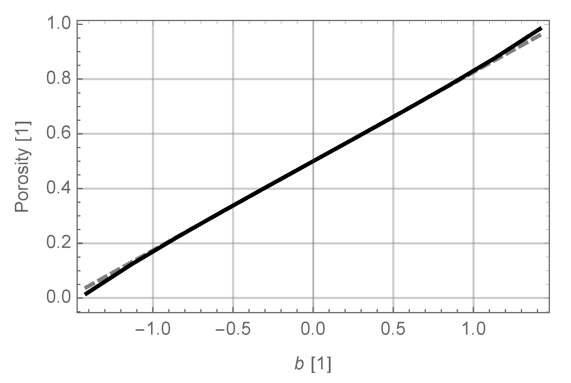
The relationship between the porosity p and the parameter b is not analytical but can be estimated numerically. As can be observed in Figure 2 this relationship is almost linear and for porosities between 0.2 and 0.8, the following linearized formula can be used to estimate the porosity:
2.2. Symmetry Properties
Thanks to its triply periodic nature, the gyroid structure can be considered as a crystal [34] with Body Centred Cubic (BCC) Bravais lattice and point group , using group theoretic notation [44], or 432 using the Hermann–Maugin notation. It should be noted that this cubic group only contains rotations geometry of the gyroid is hence chiral. To be more specific there are 3 different cubic point groups: , , and . The first one just contains rotations, the group is hence chiral and non-centrosymetric. The second, , possesses symmetry planes but not the inversion, the group is achiral and non-centrosymetric. The last group is centrosymmetric hence achiral. Some details are provided in the Appendix A, and more information can be found in [23]. The symmetry of the spatial structure is described by the space group, which details how transformations from the Bravais lattice and the point group are combined in the actual crystal. The space group () of the gyroid crystal is, using Hermann–Maugin notation, (space group #214 in the International Tables of Crystallography [45]), where the I stands for Body-Centered (BC), meaning that the conventional unit cell defined in crystallography is not primitive, but body-centered (more details provided in Section 2.3). This space group contains screw axes and, as such, is not symmorphic. A space group is called symmorphic if, apart from the lattice translations, all generating symmetry operations leave one common point fixed. Permitted as generators are thus only the point-group operations: Rotations, reflections, inversions, and rotoinversions. The symmorphic space groups may be easily identified because their Hermann–Mauguin symbol does not indicate a glide or screw operation.
If stands for the “crystal” structure, and ⭑ for the group action as defined in Appendix B:
From the generating transformations defined in Appendix B and using the equation of the gyroid surface (c.f. Equation (1)) it is straightforward to verify that:
2.3. Unit Cell
Due to the periodicity of the geometry, the study of the gyroid structure can be restricted to a unit cell:
where designates a unit cell and a periodicity lattice. Note that for a given lattice , the choice of is not unique. It can be convenient to chose a reference unit cell from which other unit cells will be defined using lattice vectors and a triplet combined as follow: . The triplet is then associated to the reference unit cell. Once a lattice basis chosen, the considered unit cell is defined as follows,
and the associated periodicity lattice is given by:
These geometrical sets can be described using lattice vectors , gathered into a basis as . Note that they can as well be described with respect to the basis of .
Among all the possible unit cells, some are special and have been given a standard name in the crystallography community: The Conventional Unit Cell (CUC) and Primitive Unit Cell (PUC).
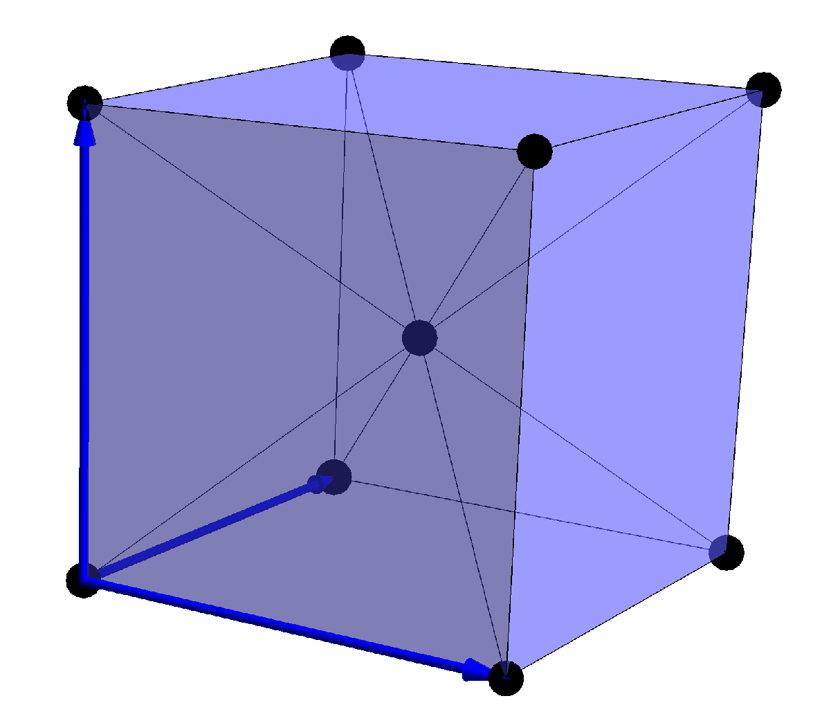
The CUC of the a BCC lattice is depicted in Figure 3. It is defined as the smallest cell having its edges along the symmetry directions of the Bravais lattice. Notice that, for BC lattice, this unit cell is not minimal and a so-called PUC can be considered instead. For a continuous structure tilling of the space, the primitive unit cell is defined as the smallest tile that generates the whole tiling using only translations. As such the primitive unit cell is a fundamental domain with respect to translational symmetries only.
2.3.1. BCC Conventional Unit Cell
For a BCC lattice, the conventional unit cell is defined as depicted in Figure 3. As its faces are perpendicular to Bravais lattice directions, despite its non minimality, this unit cell is easy to use for numerical computations.
In this case, the conventional lattice vectors , are chosen such that .
2.3.2. BCC Primitive Unit Cell
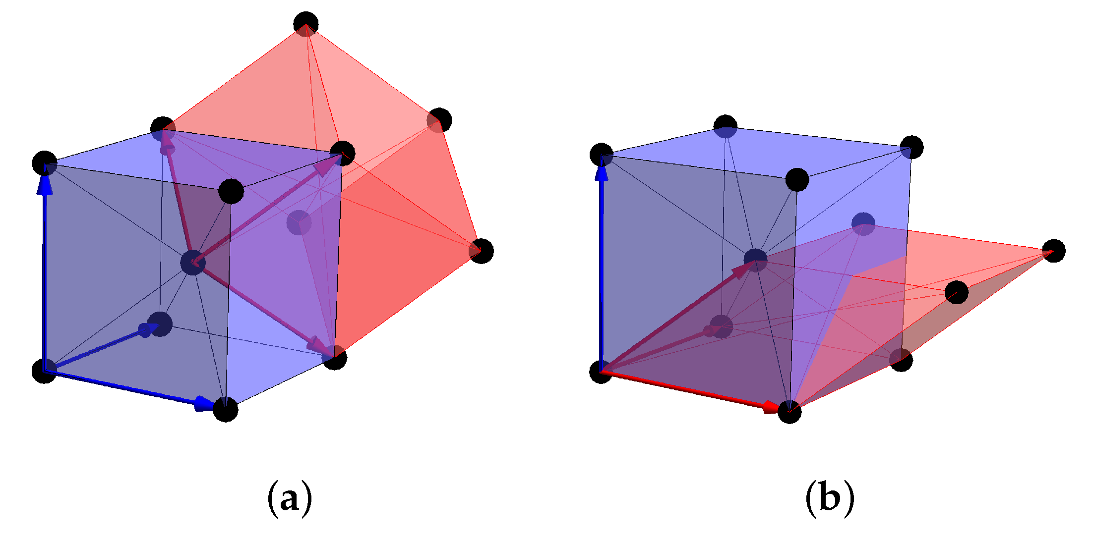
For a BCC lattice, two possible PUC are represented in Figure 4.
The primitive lattice vectors are not unique and the ones for the PUC depicted in Figure 4a are defined as:
while the ones presented in Figure 4b are defined as:
They form and two other bases of , which metric tensors are given by:
Being defined by a more symmetrical set of vectors , only the first primitive unit cell will be considered here after.
2.4. Reciprocal Basis and Brillouin Zone
The vector space dual to is symbolized by , and is formally defined as the space of linear forms on ,
Upon the choice of a scalar product the two spaces can be identified:
and from a basis of a basis of can be constructed. In the field of physics, corresponds to the space of wavevectors, and a generic element of is denoted by . For our applications, it is fundamental to introduce the reciprocal lattice of :
The vectors constitute the lattice basis of and verify:
can be computed from any lattice basis of according to:
Due to the following property,
vectors of the reciprocal lattice are the supports of -periodic functions on since,
In addition, use will be made of the First Brillouin Zone (FBZ) of the reciprocal lattice defined as:
Using the reciprocal lattice and the FBZ , any wavevector can be expressed as:
We can geometrically interpret as the set of wavevectors which are closer to the null wavevector than to any other wavevector of the reciprocal lattice . It is the Wigner–Seitz cell of the reciprocal lattice, this cell is uniquely defined and independent of the choice of . Similarly to the primitive unit cell in the direct space, the FBZ is a fundamental domain with respect to translations.
Physically, the wavelength is defined as the inverse of the wavenumber, which is the norm of the wavevector: . Then, wavevectors belonging to have wavelengths that are greater than the wavelength of the periodicity lattice. When the wavelength becomes infinite, solicitations varying with almost null wavenumber are said to be scale separated with respect to the periodicity lattice. This is usually the regime in which the LW approximation of elastodynamics homogenization holds.
The FBZ can be further reduced if we consider also the symmetry operations of the point group. The result is an Irreducible Brillouin Zone (IBZ), that is delimited by points of high symmetry, summarized for the considered gyroid lattice in Table 1. In this table, the high symmetry points are given in the non-orthogonal reciprocal lattice basis , dual to the primitive lattice basis as well as in the orthonormal lattice basis which coincides with its dual in the reciprocal space. The path obtained connecting these high symmetry points along the edges of the IBZ is often used to characterize the photonic and phononic properties of the lattice [6,26]. However, it has been pointed out that this choice is not always reliable as some relevant information, e.g., about band gaps, could be missing [46].
In this paper we consider the basis , that corresponds to the one depicted in Figure 4a. The reciprocal lattice is itself a Bravais lattice, and in the case of BCC lattice, it is a Face Centered Cubic (FCC) lattice. Using Equation (6), the reciprocal basis is equal to:
The metric tensor of is the inverse of the one of :
3. Analysis Tools
In the previous section we characterized the lattice from the point of view of crystallography. In this next section we will use these results to compute the elastodynamic response of the lattice. The objective of the present section is to provide the analysis tools to be used to perform the computation and to interpret the results.
3.1. Bloch–Floquet Analysis
Since the material is periodic, the dispersion diagram will be computed using Bloch–Floquet analysis [47]. The elastodynamics equation for the periodic continuum reads:
where is the -periodic mass density and is the -periodic fourth-order elasticity tensor. As we saw in Section 2.3, each cell of the assembly can be identified by the triplet , where the triplet is conventionally assigned to the reference unit cell. The position of a point of the -cell is obtained from the position of a point in the reference unit cell by Equation (4) where . Being -periodic, and verify:
Thanks to the Bloch–Floquet theorem [47], elementary solutions to the Equation (9) over can be searched for in the form of Bloch-waves:
where is the complex polarisation vector which is -periodic in space and constant in time, f is the frequency of the Bloch-wave, and its wavevector describes the movement of matter as the wave propagates. It is important to remark that wavevectors follow the so-called “crystallographer’s definition” which consists in dropping the often seen coefficient. This implies, for instance, that the norm , i.e., the wavenumber, is directly the inverse of the wavelength , which is more convenient for physical interpretation of the results. In the case of an homogeneous material the polarization vector becomes constant in space and the classical plane wave solution is retrieved. Since the displacement field in Equation (10) is complex valued, its real part should be computed in order to retrieve the physical solution.
From its definition as a Bloch-wave, the displacement at a point image of the by a translation has the following expression:
The physical meaning is that the displacement vector at two homologous points (two points and are said homologous if ) only differs by a phase factor.
Additionally, the Bloch-wave expression in Equation (10) has the interesting property to be also -periodic. Indeed, due to its -periodicity, can be decomposed as a Fourier series, leading to the equivalent expression for :
where stands for the Fourier coefficients of the series expansion. Using this particular form, the -periodicity of the Bloch-waves is easily proven using the change of variable :
The main consequence of this property is that the characterization of the elastodynamics behavior of a periodic material does not require to investigate the mechanical response to all the but can be restricted to the study of via -periodicity of the wavevector, where corresponds to the First Brillouin Zone (FBZ), as introduced in Section 2.3.
3.2. Polarization of Waves in Homogeneous Materials
Before presenting the results, it is useful to recall some definitions concerning the polarization of elastic waves in homogeneous materials. Let us go back to the Bloch-wave ansatz introduced in Equation (10), since the material is now considered homogeneous, the polarization vector is constant both in space and time. In the most general case, the complex polarization vector , that will be denoted from now on for the sake of simplicity, can be decomposed in its real and imaginary parts as follows:
An interpretation of this decomposition, and of its consequences on wave propagation, can be obtained by considering the real part of Equation (10):
Since the vectors and are independent, the polarization of the displacement can be very rich. Its precise nature is directly related to conditions on and , as summarized in Table 2. It is important to remark that different conventions are used to define the handedness of circularly polarized waves. In this paper, we will consider that a wave is right handed if it follows the curl of the fingers of a right hand whose thumb is directed towards the wave propagation, away from the source. In the table, the unit normal vector defining the direction of propagation is defined by .
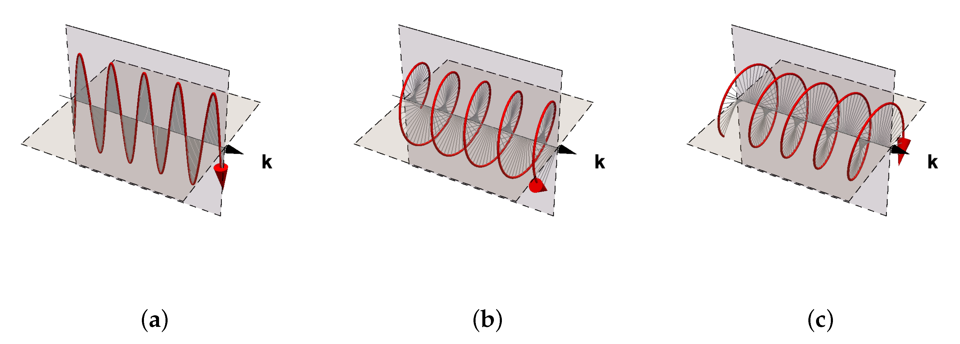
A complex polarization vector can lead to a phase shift between the components of the displacement vector , and thus to a polarization that is other than linear, see Figure 5 for illustration of a linear and two circular polarizations with opposite handedness.
4. Dispersion Analysis Using Finite Elements Analysis (FEA)
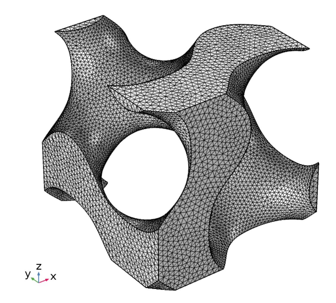
In order to investigate the ultrasonic properties of the gyroid lattice, and given the periodicity of the architecture as described in the previous sections, an approach based on Bloch–Floquet analysis will be followed. For the sake of simplicity, the conventional unit cell depicted in Figure 6 is used to define the numerical model. For the investigation of the elastodynamic properties of the gyroid crystal, the wavevector will be restricted to the boundaries of the Irreducible Brillouin Zone (IBZ), as depicted in red in Figure 7a. The high symmetry points of this IBZ are defined in Table 1. The model has been implemented using the commercial software Comsol Multiphysics and considering titanium as constitutive material, the parameters of which are displayed in Table 3. The mesh of the unit cell is presented in Figure 6 and consists of 66,232 tetrahedral elements. Lagrange quadratic elements are used, for a total of 329,277 degrees of freedom. Periodic Bloch–Floquet conditions are implemented by imposing them as displacement conditions at the boundaries, following Equation (11). Then, the wavenumber in is imposed and the corresponding frequencies are retrieved by solving the eigenvalue problem. The computation of each wavenumber took an average of 109 seconds on a workstation equipped with an Intel(R) Xeon(R) CPU E5-1650 v2 at 3.50 GHz using six cores.
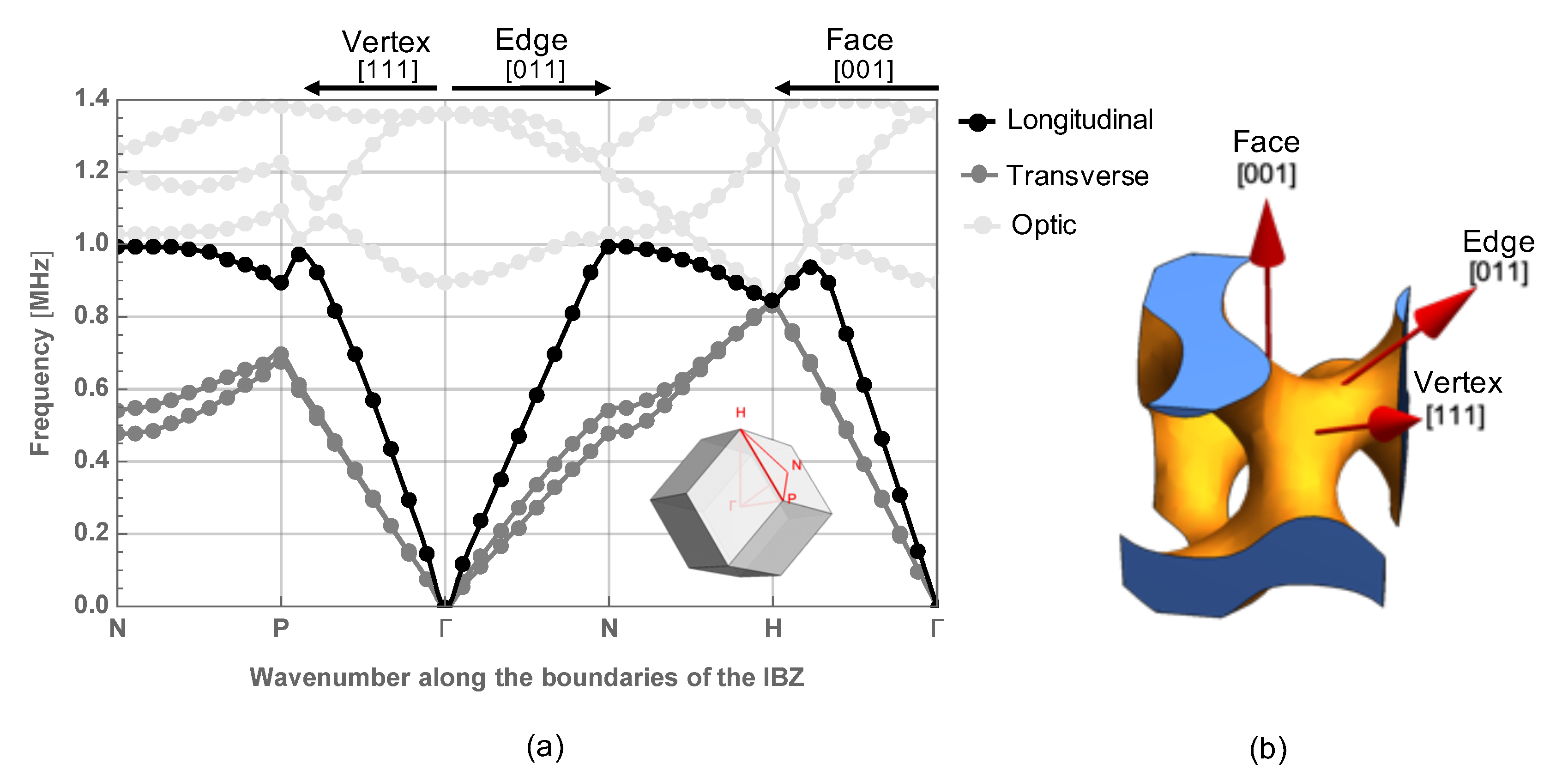
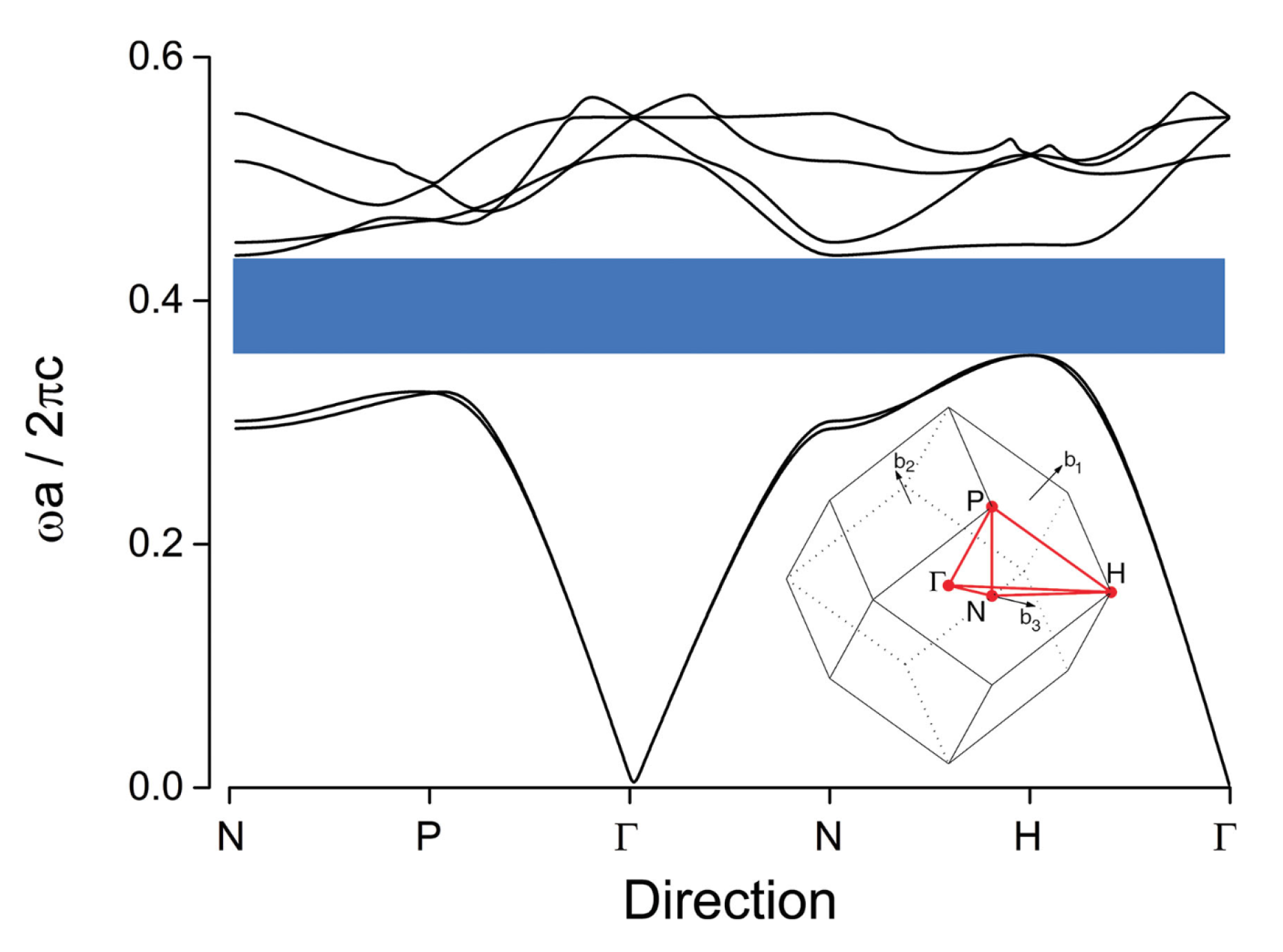
The results of the dispersion analysis are depicted in Figure 7a. It can be observed, qualitatively, that these results are similar to those obtained for electromagnetic waves in [6] (see Figure 8). In particular, the behavior of the acoustic branches, i.e., those branches starting from the origin , corresponding to transverse waves (gray lines in Figure 7a) is remarkably similar.
Since the objective of the paper is to investigate the behavior of the lattice within the LW-LF approximation given by classic continuum mechanics, the phase velocities and polarization of waves have been computed for large values of the wavelength with respect to the size of the unit cell. In this case, m, which corresponds to a wavelength close to 60 times the size of the unit cell. For each mode, the polarization vector has been estimated by computing the average of the complex displacement of the eigen-mode over the unit cell, and the results are listed in Table 4. We will now analyze the results along the following directions of propagation, also depicted in Figure 7b:
- : This direction is going from the center of the fundamental cell to the middle of a face. It corresponds to an axis of rotation of order 4 (rotations of rad);
- : This direction is going from the center of the fundamental cell to the middle of an edge. It corresponds to an axis of rotation of order 2 (rotations of rad);
- : This direction is going from the center of the fundamental cell to a vertex. It corresponds to an axis of rotation of order 3 (rotations of rad).
Using the conditions listed in Table 2, we have characterized the polarization for each of the above propagation directions. The results are summarized in Table 4.
Along the direction a longitudinal wave propagating at 3018.5 m/s can be observed. The two transverse waves have eigenmodes with complex amplitude and propagate with close phase velocity that tends to a common value of of 1932.2 m/s for infinite wavelengths, as it can be also observed in Figure 9. These complex amplitudes correspond to two circularly polarized transverse waves with opposite handedness. In the direction , a longitudinal wave propagating at 3249.8 m/s can be observed. One transverse wave is linearly polarized in direction , and propagates with a phase velocity of 1931.7 m/s. The last solution corresponds again to a transverse wave, linearly polarized along , with velocity 1510.9 m/s. Finally, direction has a linearly polarized longitudinal wave at 3322.8 m/s, and two circularly polarized waves with opposite handedness and propagating with close velocity, converging to 1663.4 m/s.
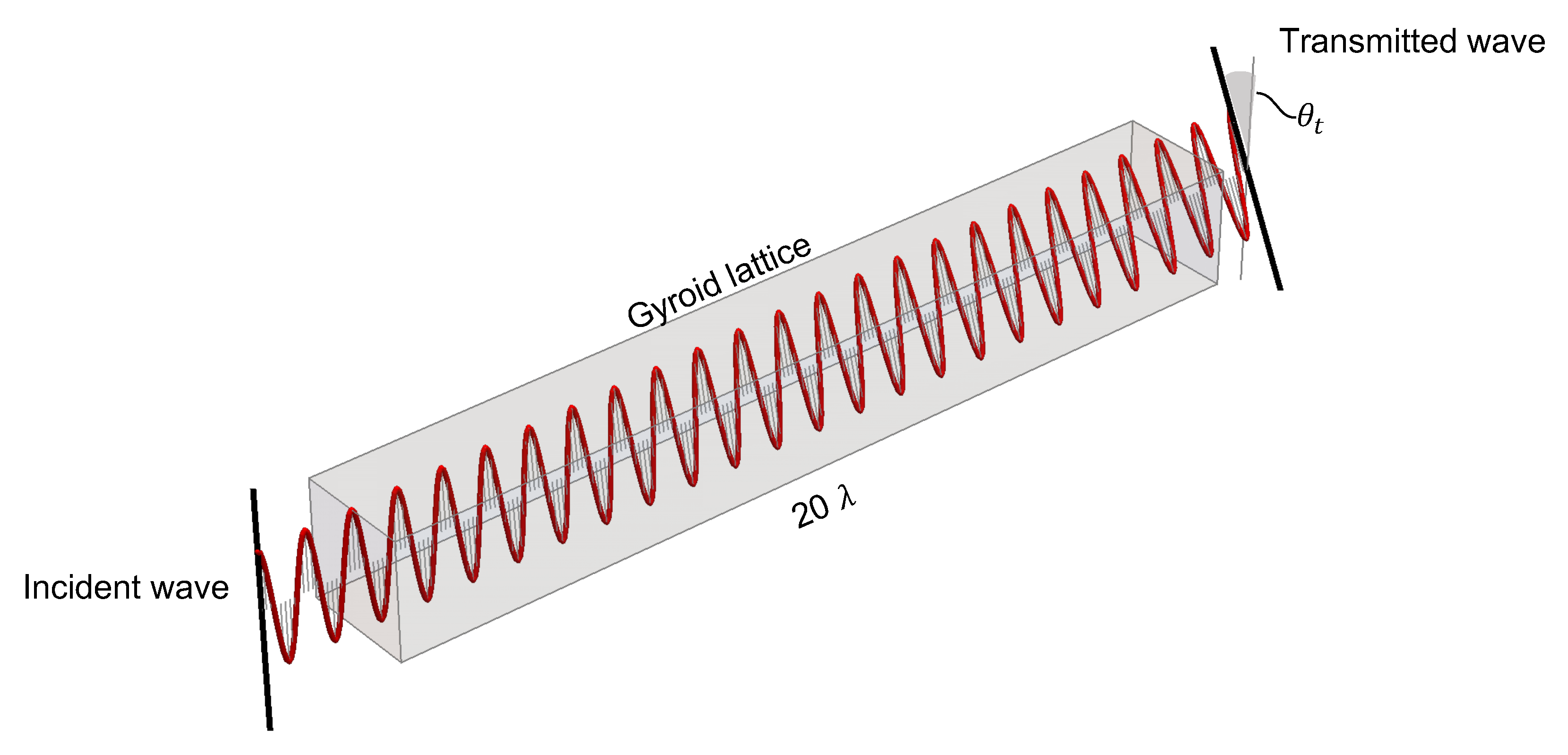
In summary, circularly polarized waves exist only if the direction of propagation is along a rotation axis of symmetry of order greater than 2. Moreover, as can be seen in Figure 9, for both and directions, the circularly polarized waves with opposite handedness propagate with the same phase velocity only in the infinite wavelength limit, and they start to diverge as the wavenumber increases. In particular, for direction the right handed wave becomes slower than the left handed one, while the opposite phenomenon can be observed for direction . This is due to the chirality of the unit cell. As one can notice, phase velocities are different even for a very large wavelength compared to the size of the unit cell, i.e., . Since only the phase velocity is affected, and not the amplitude, this effect can be interpreted as the elastic equivalent of circular birefringence in optics. This means that if a linearly polarized wave passes through a gyroid lattice, the polarization plane of the incident wave will be rotated. This is due to the phase difference (retardance) between the two circular components, which produces a rotation of the polarization plane. The concept is illustrated in Figure 10. Moreover, since phase velocity is involved in reflection of waves at boundaries via the Snell–Descartes law, and in particular in the definition of the Brewster angle of total reflection, gyroid lattices show the potential for being used as elastic circular polarizing filters.
Furthermore, the overall dispersion is normal for direction , i.e., phase velocity decreases when increasing the frequency, and anomalous for direction (see [48] for the definition). The anisotropy of the material and the dispersive properties could also have consequences on surface and guided waves propagating in presence of boundaries [49,50], as well as in reflection/transmission problems [51]. These effects will be investigated in further works.
5. Long-Wavelength and Low-Frequency Approximation and Classic Elasticity
In this last section we will introduce and identify the equivalent homogenized model in the framework of classic linear elasticity. This equivalent homogenized model is characterized by a couple of effective tensors and in such a way that the displacement field is solution of the following problem:
where verifies , denotes the spatial average operator over and is the displacement field solution to the heterogeneous problem Equation (9), as done for instance in [10].
Since the effective continuum is homogeneous, we consider a plane wave solution with where c is the phase velocity of the wave and a unitary vector. The substitution of this wave solution and of a linear elastic constitutive law into Equation (12) leads to following equation:
where is the Christoffel, or acoustic, tensor. The solution of the eigenvalue problem stated in Equation (13) for a given direction gives the phase velocities and polarizations of waves in the effective continuum.
In classical elasticity, a material with cubic symmetry is defined by three independent material constants. Using Mandel notation [52], the corresponding elastic tensor for a material having its symmetry axis parallel to reads:
It is worth noting that classical elasticity is insensitive to the lack of centrosymmetry [53]. The symmetry class of the elasticity tensor in the cubic system is meaning that even if the material symmetry group of the unit cell does not contain the inversion, the symmetry group of elasticity tensor will inherit it.
In the case of cubic materials, the solutions of Equation (13) listed in Table 5 are directly obtained.
Using the phase velocities computed from the Bloch–Floquet analysis, parameters , , , and can be identified and the homogeneous equivalent properties listed in Table 6 are then deduced. It can be noticed that, as presented in Table 5, since we considered the propagation along the rotational axes of symmetry, for each direction we observe a purely longitudinal wave and two purely transverse waves.
We now move on to comparing phase velocities and polarizations obtained from the Bloch–Floquet analysis with the ones forecast by the Long-Wavelength and Low-Frequency approximation using classical elasticity. We start with direction . As already mentioned, this direction corresponds to a rotational axis of symmetry of order 4. In this case, as the elasticity tensor is non sensitive to chirality, the symmetry group of the physical phenomenon (the symmetry group of the physical phenomenon is the intersection of the symmetry group of the constitutive equations and the symmetry group of the mechanical solicitation) is conjugate to . Indeed, as the acoustic tensor defined in Equation (13) is a second-order tensor, the Hermann theorem of Crystal physics [11] predicts its behavior as transversely isotropic, i.e., . As a consequence must have an eigenspace of dimension 2. All the directions of wave propagation for which this is verified are called acoustic axis of the material. Moving to the results presented in Table 5, we can see that the classic theory indeed predicts one faster longitudinal wave and two slower transverse waves propagating with the same phase velocity.
In the previous section we saw that Bloch–Floquet analysis identifies these waves as circularly polarized with opposite handedness, which is of course equivalent. Indeed, even for very large wavelengths, the numeric evaluation of the polarization provided by Table 4 corresponds to the eigensystem (eigenvalues plus eigenvectors) of a Hermitian acoustic tensor. In such case, the space corresponding to the double eigenvalue (which is real due to Hermitian nature of the matrix) is two dimensional over the complex field . However, in the case of a classic Cauchy continuum the acoustic tensor is symmetric real, and the eigen-space corresponding to the double eigenvalue is two dimensional over the real field . Since the 2D vector space over can be considered as a four dimensional vector space over the span is not equivalent. Moreover, as presented in Section 4, when the ratio between the wavelength and the size of the unit cell becomes finite, this 2D eigenspace splits into two 1D eigenspaces with different phase velocities. It is important to notice again that this effect occurs in the LF-LW regime, where the classical elastodynamic homogenization is supposed to hold, or give at least approximated results while preserving the physics of the problem. Similar results are obtained for propagation along , which corresponds to the rotational axis of symmetry of order 3. In this case the symmetry group of the physical phenomenon is conjugate to , and thus again transverse isotropy is imposed to the acoustic tensor. Finally, the direction of propagation is along to a rotation axis of symmetry of order 2, the physical point group is thus conjugate to . Here, the symmetry class of the acoustic tensor is , and all the eigenspaces are unidimensional. In this last case, as this kind of symmetry can be seen by second order tensors, the results from FEA on the heterogeneous material and classic elasticity are in agreement in the LF-LW regime.
In this section we have shown that some discrepancies can be observed when using an overall homogeneous continuum of Cauchy type. Classical elasticity (as opposed to generalized elasticity) is not rich enough to capture certain specific physical phenomena related to the symmetries of the material. In particular, if phase velocities are correctly estimated the polarizations are incorrectly predicted. Moreover, as it is well known, the onset of dispersion when frequency or wavenumber increase cannot be described in the classic Cauchy model.
6. Conclusions
In this work it was shown that a classical continuum model could not capture the correct behavior of elastic waves propagating in gyroid lattices. This is due to the fact that the classic continuum mechanics was insensitive to the lack of centrosymmetry of the architectured material. However, it is a well-established belief that the effects of non-centrosymmetry are only related to waves having a wavelength which compares to the size of the microstructure. Here we demonstrate that the solution given by the classical theory failed to predict the correct response, even in the Long Wavelength-Low Frequency domain.
In order to capture the onset of this unconventional behavior, called acoustical activity, the elastic continuum model needs to be enriched. Different strategies of enrichment are possible. In particular, the use of strain-gradient elasticity will be investigate in a forthcoming study.
The main practical consequence of the results presented in this work was in the evidence that circularly polarized waves could be observed in gyroid lattices, and that classic models failed to describe such effect. This could have a practical interest, since devices based on manipulation of circular polarization are frequently used in optics and electromagnetism. However, if one wants to exploit the same effects in mechanics, it appears important not to rely on classical theories of elasticity. Finally, it should be noted that, in this work, we addressed bulk wave propagation in an infinite medium. The interaction of these waves with boundaries, in the case of reflection/transmission problems or in the case of guided propagation, also deserves to be investigated.
Author Contributions
Conceptualization, G.R., N.A. and C.C.; Formal analysis, G.R., N.A. and C.C.; Methodology, G.R., N.A. and C.C.; Validation, G.R.; Software, G.R.; Writing—original draft, G.R., N.A. and C.C.; Writing—review & editing, G.R., N.A. and C.C. All authors have read and agreed to the published version of the manuscript.
Funding
The authors acknowledge the support of the French Agence Nationale de la Recherche (ANR), under grant ANR-19-CE08-0005 (project MaxOasis). This work was partially funded by CNRS/IRP Coss&Vita between Fédération Francilienne de Mécanique (F2M, CNRS FR2609) and M&MoCS.
Conflicts of Interest
The authors declare no conflict of interest.
Abbreviations
The following abbreviations are used in this manuscript:
| BCC | Body Centered Cubic |
| BZ | Brillouin Zone |
| IBZ | Irreducible Brillouin Zone |
| FEA | Finite Elements Analysis |
| FCC | Face Centered Cubic |
| LF | Low Frequency |
| LW | Long Wavelength |
Appendix A. Dictionary
To obtain the normal forms for the different classes the generators provided in the following table have been used:

Table A1.
The set of group generators used to construct matrix representation for each symmetry class.
Table A1.
The set of group generators used to construct matrix representation for each symmetry class.
| Group | Generators |
|---|---|
Where the following elements of will be used in this study:
- the rotation about through an angle ;
- the reflection through the plane normal to ().
Type I Subgroups
Table A2.
Dictionary between different group notations for Type I subgroups. The last column indicates the nature of the group: C = Chiral, P = Polar, I = Centrosymetric, and overline indicates that the property is missing.
Table A2.
Dictionary between different group notations for Type I subgroups. The last column indicates the nature of the group: C = Chiral, P = Polar, I = Centrosymetric, and overline indicates that the property is missing.
| System | Hermann−Maugin | Nature | ||
|---|---|---|---|---|
| Triclinic | CP | |||
| Monoclinic | CP | |||
| Orthotropic | C | |||
| Trigonal | CP | |||
| Trigonal | C | |||
| Tetragonal | CP | |||
| Tetragonal | C | |||
| Hexagonal | CP | |||
| Hexagonal | C | |||
| CP | ||||
| C | ||||
| Cubic | C | |||
| Cubic | C | |||
| C | ||||
| C |
Type II Subgroups
Table A3.
Dictionary between different group notations for Type II subgroups. The last column indicates the nature of the group: C = Chiral, P = Polar, I = Centrosymetric, and overline indicates that the property is missing.
Table A3.
Dictionary between different group notations for Type II subgroups. The last column indicates the nature of the group: C = Chiral, P = Polar, I = Centrosymetric, and overline indicates that the property is missing.
| System | Hermann−Maugin | Nature | ||
|---|---|---|---|---|
| Triclinic | I | |||
| Monoclinic | I | |||
| Orthotropic | I | |||
| Trigona | I | |||
| Trigonal | I | |||
| Tetragonal | I | |||
| Tetragonal | I | |||
| Hexagonal | I | |||
| Hexagonal | I | |||
| I | ||||
| I | ||||
| Cubic | I | |||
| Cubic | I | |||
| I | ||||
Type III Subgroups
Table A4.
Dictionary between different group notations for Type III subgroups. The last column indicates the nature of the group: C = Chiral, P = Polar, I = Centrosymetric, and overline indicates that the property is missing.
Table A4.
Dictionary between different group notations for Type III subgroups. The last column indicates the nature of the group: C = Chiral, P = Polar, I = Centrosymetric, and overline indicates that the property is missing.
| System | Hermann−Maugin | Nature | ||
|---|---|---|---|---|
| Monocinic | P | |||
| Orthotropic | P | |||
| Trigonal | P | |||
| Tetragonal | ||||
| Tetragonal | P | |||
| Tetragonal | ||||
| Hexagonal | ||||
| Hexagonal | P | |||
| Hexagonal | ||||
| Cubic | ||||
| P |
Appendix B. Generators of Space Group #214
Consider the affine space , the vector space acts on by translations. The affine group of , which is the set of all affine invertible transformations is constructed as the semidirect product of by , the general linear group of :
as such, an affine transformation is given by a pair . Composition of transformations follows from the construction of as a semi-direct product, to be explicit:
Elements of can be nicely represented by block matrices:
the internal law in following the matrix product in .
For our needs, we are interested not in the full affine group but in the group of isometries of , this group is a subgroup of and defined as the semi direct product of the orthogonal group and the spatial translation of :
Space groups can be considered as discrete subgroups of .
The generators of the space group (No. 214) are given in the following table in various notations [54]:
Table A5.
Generators of Group (No. 214).
| Seitz | Math | Matrices in Conventional Basis B |
|---|---|---|
Appendix C. Proof
The gyroid lattice is defined from an implicit equation (Equation (1)) that creates a periodic surface. For a given value of parameter b (=), this surface is found to become singular, thus creating an unrealistic discontinuous solid. This section presents an explanation for the admissible variation range of gyroid parameter:.
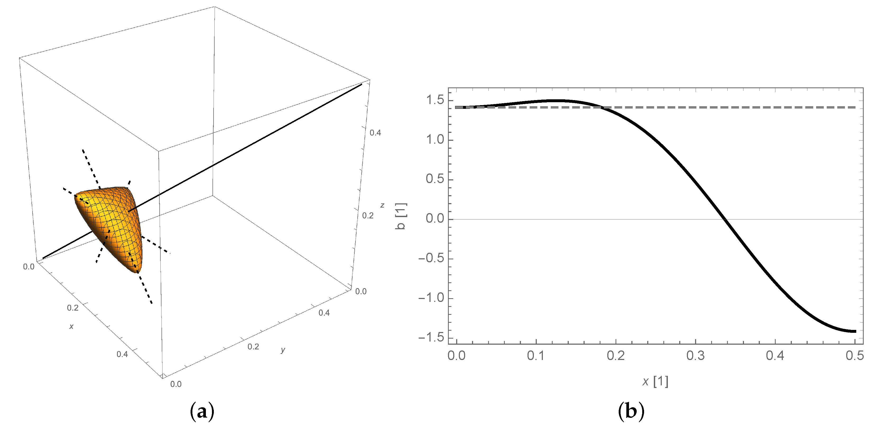
Let us first restrict the variation range of variables in Equation (2) to in order to work in the fundamental domain of function . The gyroid lattice restricted to this domain is presented in Figure A1a).
Figure A1.
(a) The gyroid restricted to its fundamental domain along with symmetry axes (plain) and (dashed) and (b) evolution of parameter b as a function of x position along axis, dashed line corresponds to .
Figure A1.
(a) The gyroid restricted to its fundamental domain along with symmetry axes (plain) and (dashed) and (b) evolution of parameter b as a function of x position along axis, dashed line corresponds to .

The fundamental domain of the gyroid is invariant with respect to the following symmetry operations:
- -
- Rotation of angle along the axis defined by equations , plotted in plain line in Figure A1 and corresponding to the transformation . The directing vector of this axis is in orthonormal basis and passes through point ;
- -
- Three rotations of angle about the three axes defined by equations , , and and plotted in dashed lines in Figure A1. These axes correspond to transformations , , , respectively. The directing vector of these axes are, in orthonormal basis , , and and they pass through points , and , respectively.
It is trivial to see that these transformations leave Equation (2) unchanged thus defining symmetry operations. As a consequence, the point symmetry group of the fundamental domain of the gyroid is conjugated to . For the sake of simplicity, we will only consider generating operations of rotation about axis and rotation about axis, denoted and in the following, respectively; the two other rotations being generated by combination of these two generators.
If the gyroid surface intersects one of the rotation axes non-orthogonally, then the surface automatically becomes degenerate. The expression of the normal director to the gyroid surface at its intersection point with generating symmetry axes and the equation defining this intersection point are summarized in the following Table A6:
Table A6.
The expression of the normal director to the gyroid surface at the intersection point with its symmetry axes and expression of this intersection point.
Table A6.
The expression of the normal director to the gyroid surface at the intersection point with its symmetry axes and expression of this intersection point.
| Sym. axis & Directing Vector | Normal to the Gyroid Surface | Intersection Point |
|---|---|---|
| with | ||
| with |
Note that the normal director to the gyroid surface depends on variable x which, itself, is determined by parameter b through the non-linear equation defining the intersection point at which the normal director is computed.
One can easily check that the normal directors are generically colinear with directing vectors of and operations. However, for given values of variable x (or equivalently of parameter b), the normal to the gyroid surface is null, thus leading to singularity of the gyroid surface. These values are –and thus –leading to singularity of the gyroid surface at its intersection with axis and –and thus –leading to singularity of the gyroid surface at its intersection with both axes.
Finally, the equation defining the intersection point between the gyroid surface and the axis (see Figure A1b) depends on x and parameter b: . By plotting this equation considering b as a function of x, we can see that there are two intersection points between the gyroid surface and the axis for values of b over thus showing that the gyroid surface forms a closed domain in these directions leading to an unrealistic discontinuous solid.
References
- Schaedler, T.A.; Carter, W.B. Architected Cellular Materials. Annu. Rev. Mater. Res. 2016, 46, 187–210. [Google Scholar] [CrossRef]
- Ashby, M.; Bréchet, Y. Designing hybrid materials. Acta Mater. 2003, 51, 5801–5821. [Google Scholar] [CrossRef]
- Fratzl, P.; Weinkamer, R. Nature’s hierarchical materials. Prog. Mater. Sci. 2007, 52, 1263–1334. [Google Scholar]
- Estrin, Y.; Bréchet, Y.; Dunlop, J.; Fratzl, P. Architectured Materials in Nature and Engineering; Springer: Berlin/Heidelberg, Germany, 2019. [Google Scholar]
- Hales, T.C. The Honeycomb Conjecture. Discret. Comput. Geom. 2001, 25, 1–22. [Google Scholar] [CrossRef] [Green Version]
- Dolan, J.A.; Wilts, B.D.; Vignolini, S.; Baumberg, J.J.; Steiner, U.; Wilkinson, T.D. Optical Properties of Gyroid Structured Materials: From Photonic Crystals to Metamaterials. Adv. Opt. Mater. 2015, 3, 12–32. [Google Scholar] [CrossRef] [Green Version]
- Wilts, B.D.; Michielsen, K.; Raedt, H.D.; Stavenga, D.G. Iridescence and spectral filtering of the gyroid-type photonic crystals in Parides sesostris wing scales. Interface Focus 2012, 2, 681–687. [Google Scholar] [CrossRef] [PubMed] [Green Version]
- Boutin, C.; Auriault, J. Rayleigh scattering in elastic composite materials. Int. J. Eng. Sci. 1993, 31, 1669–1689. [Google Scholar]
- Parnell, W.; Abrahams, I. Homogenization for wave propagation in periodic fibre-reinforced media with complex microstructure. i—theory. J. Mech. Phys. Solids 2008, 56, 2521–2540. [Google Scholar] [CrossRef]
- Nassar, H.; He, Q.C.; Auffray, N. Willis elastodynamic homogenization theory revisited for periodic media. J. Mech. Phys. Solids 2015, 77, 158–178. [Google Scholar] [CrossRef] [Green Version]
- Hermann, C. Tensoren und Kristallsymmetrie. Zeitschrift Kristallogr. 1934, 32–48. [Google Scholar] [CrossRef]
- Olive, M.; Auffray, N. Symmetry classes for even-order tensors. Math. Mech. Complex Syst. 2013, 1, 177–210. [Google Scholar] [CrossRef]
- Olive, M.; Auffray, N. Symmetry classes for odd-order tensors. ZAMM J. Appl. Math. Mech. Z. Für Angew. Math. Und Mech. 2014, 94, 421–447. [Google Scholar] [CrossRef] [Green Version]
- DiVincenzo, D.P. Dispersive corrections to continuum elastic theory in cubic crystals. Phys. Rev. B 1986, 34, 5450–5465. [Google Scholar] [CrossRef] [PubMed]
- Auffray, N.; Dirrenberger, J.; Rosi, G. A complete description of bi-dimensional anisotropic strain-gradient elasticity. Int. J. Solids Struct. 2015, 69–70, 195–206. [Google Scholar] [CrossRef]
- Rosi, G.; Auffray, N. Anisotropic and dispersive wave propagation within strain-gradient framework. Wave Motion 2016, 63, 120–134. [Google Scholar] [CrossRef] [Green Version]
- Eremeyev, V.A. On the material symmetry group for micromorphic media with applications to granular materials. Mech. Res. Commun. 2018, 94, 8–12. [Google Scholar] [CrossRef]
- Eremeyev, V.A.; Rosi, G.; Naili, S. Comparison of anti-plane surface waves in strain-gradient materials and materials with surface stresses. Math. Mech. Solids 2018, 24, 2526–2535. [Google Scholar] [CrossRef]
- Eremeyev, V.A.; Rosi, G.; Naili, S. Transverse surface waves on a cylindrical surface with coating. Int. J. Eng. Sci. 2019, 103188. [Google Scholar] [CrossRef]
- Arago, F. Mémoire sur une Modification Remarquable Qu’éProuvent Les Rayons Lumineux Dans Leur Passage à Travers Certains Corps Diaphanes et sur Quelques Autres Nouveaux Phénomènes D’Optique; Institut National de France: Paris, France, 1811; Volume 1, pp. 93–134. [Google Scholar]
- Portigal, D.L.; Burstein, E. Acoustical Activity and Other First-Order Spatial Dispersion Effects in Crystals. Phys. Rev. 1968, 170, 673–678. [Google Scholar] [CrossRef]
- Sivardière, J. Description de la Symétrie; EDP: Ulysse, France, 2004. [Google Scholar]
- Auffray, N.; He, Q.C.; Le Quang, H. Complete symmetry classification and compact matrix representations for 3D strain gradient elasticity. Int. J. Solids Struct. 2019, 159, 197–210. [Google Scholar] [CrossRef] [Green Version]
- Prall, D.; Lakes, R.S. Properties of a chiral honeycomb with a Poisson’s ratio of—1. Int. J. Mech. Sci. 1997, 39, 305–307, 309–314. [Google Scholar] [CrossRef]
- Lakes, R. Elastic and viscoelastic behavior of chiral materials. Int. J. Mech. Sci. 2001, 43, 1579–1589. [Google Scholar] [CrossRef] [Green Version]
- Spadoni, A.; Ruzzene, M.; Gonella, S.; Scarpa, F. Phononic properties of hexagonal chiral lattices. Wave Motion 2009, 46, 435–450. [Google Scholar] [CrossRef] [Green Version]
- Liu, X.N.; Hu, G.K.; Sun, C.T.; Huang, G.L. Wave propagation characterization and design of two-dimensional elastic chiral metacomposite. J. Sound Vib. 2011, 330, 2536–2553. [Google Scholar] [CrossRef]
- Liu, X.N.; Huang, G.L.; Hu, G.K. Chiral effect in plane isotropic micropolar elasticity and its application to chiral lattices. J. Mech. Phys. Solids 2012, 60, 1907–1921. [Google Scholar] [CrossRef] [Green Version]
- Dirrenberger, J.; Forest, S.; Jeulin, D. Effective elastic properties of auxetic microstructures: Anisotropy and structural applications. Int. J. Mech. Mater. Des. 2013, 9, 21–33. [Google Scholar] [CrossRef]
- Bacigalupo, A.; Gambarotta, L. Homogenization of periodic hexa-and tetrachiral cellular solids. Compos. Struct. 2014, 116, 461–476. [Google Scholar] [CrossRef] [Green Version]
- Fernandez-Corbaton, I.; Rockstuhl, C.; Ziemke, P.; Gumbsch, P.; Albiez, A.; Schwaiger, R.; Frenzel, T.; Kadic, M.; Wegener, M. New Twists of 3D Chiral Metamaterials. Adv. Mater. (Deerfield Beach, Fla.) 2019, 31, e1807742. [Google Scholar] [CrossRef] [Green Version]
- Chen, Y.; Frenzel, T.; Guenneau, S.; Kadic, M.; Wegener, M. Mapping acoustical activity in 3D chiral mechanical metamaterials onto micropolar continuum elasticity. J. Mech. Phys. Solids 2020, 103877. [Google Scholar] [CrossRef]
- Ziemke, P.; Frenzel, T.; Wegener, M.; Gumbsch, P. Tailoring the characteristic length scale of 3D chiral mechanical metamaterials. Extrem. Mech. Lett. 2019, 32, 100553. [Google Scholar] [CrossRef]
- Chen, Y.; Yao, H.; Wang, L. Acoustic band gaps of three-dimensional periodic polymer cellular solids with cubic symmetry. J. Appl. Phys. 2013, 114, 043521. [Google Scholar] [CrossRef]
- Rammohan, A.V.; Lee, T.; Tan, V.B.C. A Novel Morphological Model of Trabecular Bone Based on the Gyroid. Int. J. Appl. Mech. 2015, 07, 1550048. [Google Scholar] [CrossRef]
- Ma, S.; Tang, Q.; Feng, Q.; Song, J.; Han, X.; Guo, F. Mechanical behaviours and mass transport properties of bone-mimicking scaffolds consisted of gyroid structures manufactured using selective laser melting. J. Mech. Behav. Biomed. Mater. 2019, 93, 158–169. [Google Scholar] [CrossRef] [PubMed] [Green Version]
- Poncelet, M.; Somera, A.; Morel, C.; Jailin, C.; Auffray, N. An experimental evidence of the failure of Cauchy elasticity for the overall modeling of a non-centro-symmetric lattice under static loading. Int. J. Solids Struct. 2018, 147, 223–237. [Google Scholar] [CrossRef] [Green Version]
- Abdoul-Anziz, H.; Seppecher, P.; Bellis, C. Homogenization of frame lattices leading to second gradient models coupling classical strain and strain-gradient terms. Math. Mech. Solids 2019, 24, 3976–3999. [Google Scholar] [CrossRef] [Green Version]
- Yvonnet, J.; Auffray, N.; Monchiet, V. Computational second-order homogenization of materials with effective anisotropic strain-gradient behavior. Int. J. Solids Struct. 2020, 191, 434–448. [Google Scholar] [CrossRef]
- Schoen, A.H. Infinite Periodic Minimal Surfaces without Self-Intersections; Nasa Technical Notes TN D-5541; NTRS: Washington, DC, USA, 1970; p. 100. [Google Scholar]
- Schoen, A.H. Reflections concerning triply-periodic minimal surfaces. Interface Focus 2012, 2, 658–668. [Google Scholar] [CrossRef] [Green Version]
- Dacorogna, B. Introduction to the Calculus of Variations; World Scientific Publishing Company: Singapore, 2014. [Google Scholar]
- Wohlgemuth, M.; Yufa, N.; Hoffman, J.; Thomas, E.L. Triply periodic bicontinuous cubic microdomain morphologies by symmetries. Macromolecules 2001, 34, 6083–6089. [Google Scholar] [CrossRef]
- Golubitsky, M.; Stewart, I.; Schaeffer, D.G. Singularities and Groups in Bifurcation Theory; Applied Mathematical Sciences; Springer: New York, NY, USA, 1988; Volume 69. [Google Scholar] [CrossRef]
- Hahn, T.; Shmueli, U.; Wilson, A.J.C.; Prince, E. International Tables for Crystallography; D. Reidel Publishing Company: Dordrecht, The Netherlands, 2005. [Google Scholar]
- Craster, R.V.; Antonakakis, T.; Makwana, M.; Guenneau, S. Dangers of using the edges of the Brillouin zone. Phys. Rev. B 2012, 86, 115130. [Google Scholar] [CrossRef] [Green Version]
- Gazalet, J.; Dupont, S.; Kastelik, J.C.; Rolland, Q.; Djafari-Rouhani, B. A tutorial survey on waves propagating in periodic media: Electronic, photonic and phononic crystals. Perception of the Bloch theorem in both real and Fourier domains. Wave Motion 2013, 50, 619–654. [Google Scholar] [CrossRef]
- Achenbach, J. Wave Propagation in Elastic Solids; Elsevier: Amsterdam, The Netherlands, 1984. [Google Scholar]
- Zakharenko, A.A. On cubic crystal anisotropy for waves with Rayleigh-wave polarization. Nondestruct. Test. Eval. 2006, 21, 61–77. [Google Scholar] [CrossRef]
- Rosi, G.; Nguyen, V.H.; Naili, S. Surface waves at the interface between an inviscid fluid and a dipolar gradient solid. Wave Motion 2015, 53, 51–65. [Google Scholar] [CrossRef]
- Gourgiotis, P.A.; Georgiadis, H.G.; Neocleous, I. On the reflection of waves in half-spaces of microstructured materials governed by dipolar gradient elasticity. Wave Motion 2013, 50, 437–455. [Google Scholar] [CrossRef]
- Mandel, J. Généralisation de la théorie de plasticité de WT Koiter. Int. J. Solids Struct. 1965, 1, 273–295. [Google Scholar] [CrossRef]
- Forte, S.; Vianello, M. Symmetry classes for elasticity tensors. J. Elast. 1996, 43, 81–108. [Google Scholar] [CrossRef]
- Aroyo, M.I.; Perez-Mato, J.M.; Capillas, C.; Kroumova, E.; Ivantchev, S.; Madariaga, G.; Kirov, A.; Wondratschek, H. Bilbao Crystallographic Server: I. Databases and crystallographic computing programs. Z. Für Krist. Cryst. Mater. 2006, 221, 15–27. [Google Scholar]
Figure 1.
The unit cells of gyroid lattices obtained for mm and: (a) , (b) , (c) . Despite what the angle of view may suggest, all these structures are simply connected.
Figure 1.
The unit cells of gyroid lattices obtained for mm and: (a) , (b) , (c) . Despite what the angle of view may suggest, all these structures are simply connected.

Figure 2.
The relationship between the parameter b and the porosity, dashed line represents a linear approximation of real porosity plotted in plain line. The evaluation of the porosity is obtained numerically.
Figure 2.
The relationship between the parameter b and the porosity, dashed line represents a linear approximation of real porosity plotted in plain line. The evaluation of the porosity is obtained numerically.

Figure 3.
The conventional unit cell. The lattice vectors are indicated in blue.

Figure 4.
Two examples of Primitive Unit Cells (PUC). In (a,b) the Conventional Unit Cell are in blue and the PUC are in red. The PUC in (a) is considered in the present paper, as their lattice vectors (indicated in red) are more symmetrical than those of the one in (b).
Figure 4.
Two examples of Primitive Unit Cells (PUC). In (a,b) the Conventional Unit Cell are in blue and the PUC are in red. The PUC in (a) is considered in the present paper, as their lattice vectors (indicated in red) are more symmetrical than those of the one in (b).

Figure 5.
Some examples of polarizations: (a) Linear, (b) circular right handed, and (c) circular left handed.
Figure 5.
Some examples of polarizations: (a) Linear, (b) circular right handed, and (c) circular left handed.

Figure 6.
The meshed unit cell used in simulations.

Figure 7.
The dispersion diagram of the Gyroid lattice computed along the boundaries of the Irreducible Brillouin Zone (IBZ) and directions of propagation with respect to the unit cell. (a) The dispersion relation of the Gyroid lattice computed along the boundaries of the IBZ. (b) The direction of propagation with respect to the unit cell.

Figure 8.
The photonic band diagram of a single gyroid photonic crystal. Reproduced with permission from [6].
Figure 8.
The photonic band diagram of a single gyroid photonic crystal. Reproduced with permission from [6].

Figure 9.
The phase velocity of the circularly polarized waves in function of the wavenumber or of the ratio between the wavelength and the size of the unit cell a for propagation direction (a) and (b). Right handed waves are in black, left handed waves are in gray. The dashed horizontal lines correspond to the phase velocity to which they converge to for infinite wavelength.

Figure 10.
An illustration of circular birefringence observed along direction [100] at kHz, corresponding to a wavelength around 10 times the size of the unit cell. A linearly polarized wave entering the material is subjected to a rotation of 1.3 degrees/wavelength, then after 20 wavelengths the rotation is deg. This illustration does not account for the changes in amplitude due to the reflections at boundaries.

Table 1.
The high symmetry points of the gyroid lattice. The group notations are detailed in Appendix A.
Table 1.
The high symmetry points of the gyroid lattice. The group notations are detailed in Appendix A.
| Symmetry | Coordinates | Coordinates | Point Group | Point Group | Illustration of the |
|---|---|---|---|---|---|
| Point | w.r.t. | w.r.t. | (Math.) | (H-M) | First Brillouin Zone |
| 432 |  | ||||
| H | 432 | ||||
| P | 32 | ||||
| N | 222 |
Table 2.
The polarizations of plane waves and conditions on the complex amplitude.
| Polarization | Condition |
|---|---|
| Longitudinal polarization | with |
| Transverse polarization | and belong to the plane orthogonal to |
| Linear polarization | , with complex conjugate of |
| Circular polarization | |
| ↳ Right handedness | |
| ↳ Left handedness | |
| Elliptic polarization | and |
Table 3.
The parameters used in the numerical simulations, corresponding to bulk titanium.
| Mass Density [kg/m] | Young Modulus [GPa] | Poisson Ratio [1] | Porosity [1] | Unit Cell Size [mm] |
|---|---|---|---|---|
| 4506 | 115.7 | 0.321 | 0.7 | 1 |
Table 4.
The phase velocity and polarization in the very long wavelength approximation.
| Direction | Phase Velocity | Polarization | Type of Wave |
|---|---|---|---|
| [m/s] | |||
| Longitudinal | |||
| Circular L ⥁ | |||
| Circular R ⥀ | |||
| 3249.8 | Longitudinal | ||
| 1931.7 | Transverse | ||
| 1510.9 | Transverse | ||
| 3322.8 | Longitudinal | ||
| 1664.6 | Circular R ⥀ | ||
| 1662.3 | Circular L ⥁ |
Table 5.
The phase velocity and polarization in classic elasticity.
| Direction | Phase Velocities [m/s] | Polarization | Type of Wave |
|---|---|---|---|
| Longitudinal | |||
| Transverse | |||
| Transverse | |||
| Longitudinal | |||
| Transverse | |||
| Transverse | |||
| Longitudinal | |||
| Transverse | |||
| Transverse |
Table 6.
The material properties in the very long wavelength approximation.
| Elastic Coefficients | Mass Density | ||
|---|---|---|---|
| [GPa] | [GPa] | [GPa] | [kg/m] |
| 12.32 | 6.145 | 10.092 | 1351.8 |
© 2020 by the authors. Licensee MDPI, Basel, Switzerland. This article is an open access article distributed under the terms and conditions of the Creative Commons Attribution (CC BY) license (http://creativecommons.org/licenses/by/4.0/).
Share and Cite
MDPI and ACS Style
Rosi, G.; Auffray, N.; Combescure, C. On the Failure of Classic Elasticity in Predicting Elastic Wave Propagation in Gyroid Lattices for Very Long Wavelengths. Symmetry 2020, 12, 1243. https://doi.org/10.3390/sym12081243
AMA Style
Rosi G, Auffray N, Combescure C. On the Failure of Classic Elasticity in Predicting Elastic Wave Propagation in Gyroid Lattices for Very Long Wavelengths. Symmetry. 2020; 12(8):1243. https://doi.org/10.3390/sym12081243
Chicago/Turabian StyleRosi, Giuseppe, Nicolas Auffray, and Christelle Combescure. 2020. "On the Failure of Classic Elasticity in Predicting Elastic Wave Propagation in Gyroid Lattices for Very Long Wavelengths" Symmetry 12, no. 8: 1243. https://doi.org/10.3390/sym12081243
Note that from the first issue of 2016, this journal uses article numbers instead of page numbers. See further details here.