Off-Shell Quantum Fields to Connect Dressed Photons with Cosmology

Abstract

The anomalous nanoscale electromagnetic field arising from light–matter interactions in a nanometric space is called a dressed photon. While the generic technology realized by utilizing dressed photons has demolished the conventional wisdom of optics, for example, the unexpectedly high-power light emission from indirect-transition type semiconductors, dressed photons are still considered to be too elusive to justify because conventional optical theory has never explained the mechanism causing them. The situation seems to be quite similar to that of the dark energy/matter issue in cosmology. Regarding these riddles in different disciplines, we find a common important clue for their resolution in the form of the relevance of space-like momentum support, without which quantum fields cannot interact with each other according to a mathematical result of axiomatic quantum field theory. Here, we show that a dressed photon, as well as dark energy, can be explained in terms of newly identified space-like momenta of the electromagnetic field and dark matter can be explained as the off-shell energy of the Weyl tensor field.

1. Introductory Review of Dressed Photon Technology

1.1. Broad Overview

Suppose that a nanometer-sized material (NM) is illuminated by propagating light whose diffraction-limited size is much larger than the size of the NM. Then, an anomalous non-propagating localized light field is generated around the NM, contrary to the accepted knowledge of optics. This non-propagating light field is called the optical near field [1], which is undetectable by a separately placed conventional photodetector. The studies on the optical near field initiated practically in the late 20th century have led, through trial-and-error approaches, to the novel concept of a quasi-particle created as a result of light–matter interaction in a nanometric space. This quasi-particle is figuratively called the dressed photon (DP), that is, a metaphoric expression of photon energy partly fused with the energies of the material involved in the interaction. Figure 1 shows typical experimental setups for creating a DP. Studies on DPs are now rapidly progressing, yielding innovative generic technologies [2] of “small light”, which accomplish the impossible in a variety of application fields.

One should bear in mind, however, that the concept of a DP first proposed by one of the authors (M.O.) still seems to be either ignored or tacitly understood differently by the mainstream researchers in optical sciences because of the conceptual difficulty of dealing with off-shell quantities in the midst of field interactions. We think that this kind of refusal or confusion about DPs stems from a certain degree of ambiguity in using such an abstract expression as light–matter field interactions in a nanometric space; the main purpose of the above remark is not to criticize the incorrect usage of DPs in the literature but rather to promote renewed awareness that the issue of DP phenomena addressed here is a remarkable one that cannot be understood within the conventional framework of optical theory.

To elucidate the essence of the DP problem, we start by listing five conventional views in optics and briefly show how a DP violates them.

Five conventional common views in optics

I. 

Light is a propagating wave that fills a space. Its spatial extent (size) is much larger than its wavelength.

II. 

Light cannot be used for imaging and fabrication of sub-wavelength-sized materials. Furthermore, light cannot be used for assembling and operating sub-wavelength-sized optical devices.

III. 

For optical excitation of an electron, the photon energy must be equal to or higher than the energy difference between the relevant two electronic energy levels.

IV. 

An electron cannot be optically excited if the transition between the two electric energy levels is electric dipole forbidden.

V. 

Crystalline silicon has a very low light emission efficiency and is thus unsuitable for use as an active medium in light-emitting devices.

Contrary to I–V above, the intrinsic natures of DPs have enabled the advent of innovative technologies such as the following: (1) Nanometer-sized optical devices. These devices are operated on the basis of the spatially localized nature of DPs created on an NM (Figure 1a) and the autonomous DP energy transfer between NMs. These devices are based on the intrinsic nature of a DP that is contrary to I, II and IV. Integrated 2D arrays of NOT- and AND-logic gates operating at room temperature have been fabricated using InAs NMs [3]. (2) Nanofabrication technology, such as chemical vapor deposition and autonomous smoothing of a material surface (Figure 1b,c). These technologies are based on the intrinsic nature of a DP that is contrary to I–IV. Their details will be described in subsection 1.2 since the information on the maximum size of a DP will be used in Section 4 on cosmology. (3) Light-emitting devices using indirect-transition-type semiconductors. These devices are based on the intrinsic nature of a DP that is contrary to V. Infrared light-emitting diodes using crystalline silicon (Si) have been realized. For their fabrication, a method of DP-assisted annealing has been invented to autonomously control the spatial distribution of the dopant atoms on which DPs are created and localized (Figure 1d). Their output optical powers are as high as 2 W [4]. Infrared Si lasers have also been developed whose CW output optical power is as high as 100 W, and the threshold current density is as low as 60 A/cm [2] at room temperature [5]. Their high power and low energy consumption factors are ${10}^4$ and 0.05, respectively, relative to those of the conventional single-stripe double heterojunction-structured semiconductor lasers fabricated using the direct-transition-type compound InGaAsP. Furthermore, novel polarization rotators have been developed using crystalline SiC that exhibit a gigantic ferromagnetic magneto-optical effect [6].

1.2. Nanofabrication Technology and the Size of a DP

This subsection describes two examples of nanofabrication technology that provide key experimental data for theoretical discussions in Section 2, Section 3 and Section 4. In particular, the maximum size of a DP was determined by analyzing a large number of experimental results.

1.2.1. Photochemical Vapor Deposition

In this method, a material is grown by depositing atoms on a substrate. Gaseous molecules are dissociated when a DP is created, for example, on the fiber probe tip of Figure 1b. Atoms created by this dissociation are deposited on the substrate installed below the fiber probe tip. Since the size of a DP is equivalent to that of the fiber probe tip, a sub-wavelength-sized NM can be grown, which is contrary to common views I and II. Furthermore, the photon energy $h{\nu }_{in}$ of the light incident on the end of the fiber probe can be lower than the excitation energy $E_{excite}$ of the electrons in the molecule, which is contrary to common view III. This phenomenon occurs because the energy $h{\nu }_{DP}$ of the created DP is given by the sum of $h{\nu }_{in}$, the energies of excitons and phonons in the fiber probe, and thus $h{\nu }_{DP}\ge E_{excite}$. For example, DP dissociated gaseous Zn(C${}_2$H${}_5$)${}_2$ molecules (the wavelength ${\lambda }_{excite}$ of light whose energy corresponds to $E_{excite}$ was as short as 270 nm), thus depositing an NM composed of Zn atoms on a sapphire substrate. In contrast to common view III, blue incident light (wavelength ${\lambda }_{in}=488$ nm $>{\lambda }_{excite}$) was used. Figure 2a shows 3D atomic force microscopic (AFM) images of the grown NMs [7]. Furthermore, the electric dipole-forbidden transition of electrons could be used for dissociation, which is contrary to common view IV. This approach was possible because the conventional long-wave approximation is not valid in the case of a DP due to its sub-wavelength size. For example, DPs dissociated optically inactive Zn(acac)${}_2$ molecules, thus depositing Zn atoms, using visible incident light (457 nm wavelength) (Figure 2b) [8,9].

The maximum size of a DP was estimated by measuring temporal variations in the deposition rate of the number of Zn atoms and the full-width at half-maximum (FWHM) of the 3D image [10]. The results showed that, in the initial stage of deposition, the deposition rate and the FWHM increased monotonically with time. When the FWHM reached the size of the fiber probe tip, the deposition rate was the maximum, which is the phenomenon known as size-dependent resonance between the fiber probe tip and the size of the NM [11]. Then, the deposition rate monotonically decreased and approached a constant value. This result indicated that the size of the NM asymptotically approached a certain value. Since the height of the NM monotonically increased with the deposition time, this approach indicated that the value of the FWHM approached a certain value. To confirm this indication, the maximum value of the FWHM was evaluated from the 3D images of the saturated-sized NMs. As a result, a value of 50–70 nm was obtained after compensating for the errors and inaccuracies in the experimental data. Figure 2a,b just show the images of the NMs with the maximum value of the FWHM. This maximum value also indicated that the maximum size of a DP is 50–70 nm because the size of the DP transferred from the fiber probe tip to the NM corresponds to the size of the NM. A series of experiments confirmed that this value was independent of the molecular species, the wavelength and power of the incident light, the conformation, and the size of the fiber probe tip.

1.2.2. Smoothing Material Surfaces

Galilei chemical-mechanically polished the lens surfaces of his telescope as early as the 17th century. Although this method is popularly used even now in industry, polishing 3D or microsurfaces using this method is difficult because it is a contact method that employs a polishing pad. Furthermore, small scratches are created on the surface during the polishing process. To solve these problems, a non-contact dry-etching method was invented using DPs [12]. Its principle is nearly the same as that of the photochemical vapor deposition above. That is, DPs are created on small bumps of the rough surface by light irradiation (Figure 1c). A gaseous Cl${}_2$ molecule, as an example, is dissociated if it jumps into the DP field. Since the created Cl atom is chemically active, it etches the bump without using any devices such as a fiber probe. Thus, etching autonomously starts upon light irradiation, varying the conformation and size of the bumps, and stops when the surface becomes flat, i.e., when DPs are no longer created. A variety of 3D surfaces, such as convex surfaces, concave surfaces, and the side walls and inner wall of a cylinder, have been smoothed. The microsized side walls of the corrugations of a diffraction grating were also smoothed. This method has been applied to a variety of materials, such as glasses, crystals, ceramics, and plastics, to decrease the roughness to sub-nanometer. It has been employed in industry to increase the optical damage threshold of high-power UV laser mirrors [13], repair the surface of photomasks for UV lithography [14], and so on.

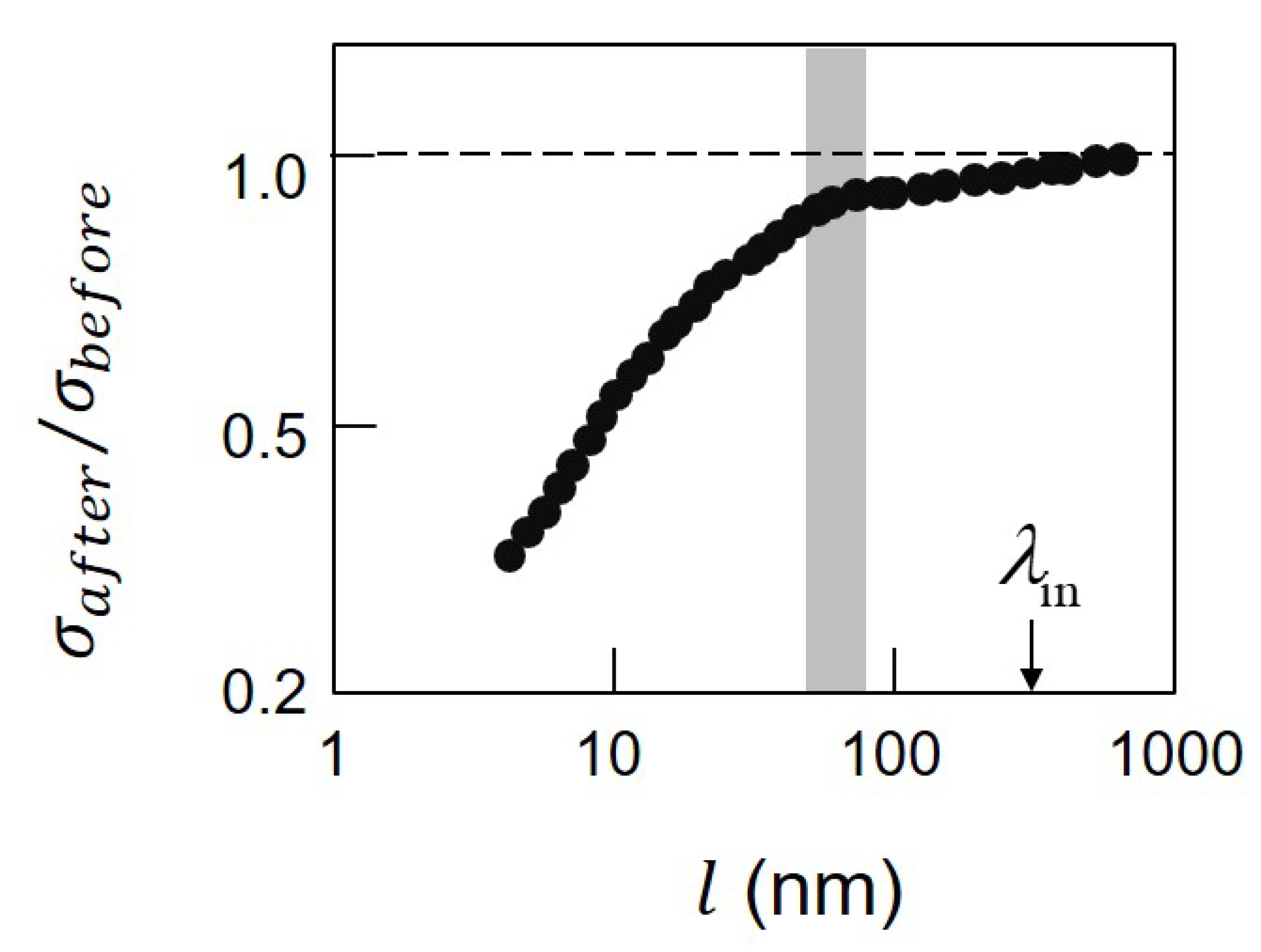
The maximum size of a DP was also evaluated by this method: Figure 3 shows the experimental results of polishing a plastic PMMA surface by dissociating O${}_2$ molecules by DPs [15]. The wavelength ${\lambda }_{excite}$ of light corresponding to the $E_{excite}$ of the O${}_2$ molecule was 242 nm. However, the wavelength ${\lambda }_{in}$ of the incident light was as long as 325 nm (>${\lambda }_{excite}$), contrary to common view III. The horizontal axis represents the period l of the surface roughness. The vertical axis is the standard deviation $\sigma$ of the roughness acquired from the AFM images. Here, the ratio ${\sigma }_{after}/{\sigma }_{before}$ between the values before (${\sigma }_{before}$) and after (${\sigma }_{after}$) the etching is plotted on a logarithmic scale. This figure shows that ${\sigma }_{after}/{\sigma }_{before}$ was less than 1 in the range of $l<$ 50–70 nm, from which the maximum size of the DP is again confirmed to be 50–70 nm, as displayed by the grey band in this figure.

For comparison, in the case when ${\lambda }_{in}=213$ nm (<${\lambda }_{excite}$), which follows common view III, the value of ${\sigma }_{after}/{\sigma }_{before}$ was less than unity only in the range of $l>{\lambda }_{in}$. In contrast, ${\sigma }_{after}/{\sigma }_{before}>1$ in the range of $l<{\lambda }_{in}$ was obtained. By comparing these results, etching by DPs is confirmed to be effective for selectively removing fine bumps of sub-wavelength size.

2. New Theory for Dressed Photon

2.1. Missing Aspect of Quantum Field Interaction Theory

In the usual quantum field theory (QFT), scattering processes are described by the LSZ reduction formulae [16], which determine the S-matrix elements $S_{\beta \alpha }$ connecting the in(-coming) and out(-going) scattering states, $|\alpha ,in\rangle$ and $|\beta ,out\rangle$, respectively, as on-shell projections of the time-ordered Green functions. This way of description is suitable for experimental situations satisfying the asymptotic completeness which means that interactions among fields can be reduced to scattering processes. In such situations, in-states $|\alpha ,in\rangle \in {\mathfrak{H}}^{in}$ describe the states of on-shell particles in the Heisenberg picture in Hilbert space $\mathfrak{H}$ before the interaction at $t=-\infty$, and out-states $|\beta ,out\rangle \in {\mathfrak{H}}^{out}$ representing the final states of on-shell particles after the interaction at $t=+\infty$, which can be determined by modeled scattering processes under the assumption $\mathfrak{H}={\mathfrak{H}}^{in}={\mathfrak{H}}^{out}$ of asymptotic completeness.

In the situations with asymptotic completeness being valid, all the discussions can safely be focused on the on-shell aspects in terms of the S-matrix for which the LSZ formulae in QFT are used commonly among particle physicists. In this case, however, an important issue has been forgotten regarding the roles played by off-shell Heisenberg fields at the center of given field interactions. We note here that the Greenberg and Robinson theorem [17,18] proved in axiomatic quantum field theory shows that an interaction among quantum fields must inevitably accompany space-like momentum supports whenever this interaction can non-trivially transform in-states of asymptotic field ${\varphi }^{in}$ into out-states of asymptotic field ${\varphi }^{out}$ describing particles with time-like momentum support. Note that space-like momentum here does not mean the presence of a tachyonic field [19] carrying unstable particles with space-like momenta.

Thus, the consequence of the axiomatic theory claiming the existence of space-like momentum support is a remarkable feature in sharp contrast to the conventional perturbative expansion method for field interactions, in which only on-shell particles with time-like or light-like momentum support are considered physical. This important result has been totally neglected thus far, perhaps owing to such prejudice that abstract consequences in mathematical theorems are irrelevant to specific physical aspects of interacting fields. In the following subsection, however, our discussion on DPs will exhibit the existence of space-like momentum supports in such a form linked to the existence of well-known $U\left(1\right)$ gauge bosons mediating electromagnetic interactions as virtual photons. Since the notion of virtual photons is closely-linked to perturbative expansion methods not necessarily related to space-like momenta of the field under consideration, the term of virtual photons mentioned above is used in a loose sense. In what follows, we are going to reexamine the problem of electromagnetic interaction from the viewpoint of Micro-Macro duality theory to be touched upon shortly below in which not only microscopic “particle modes”but also macroscopic “non-particle condensates”play key roles to attain complete description of given electromagnetic fields.

2.2. Augmented Maxwell’s Equation

In view of the unfamiliarity in the science community at large with the relevant subjects, we recapitulate the important points to make this article self-contained, on the basis of [5], the latest tutorial paper on DPs, which summarizes most of the results reported in a series of works [5,20,21,22]. In our new theory on DPs, we have introduced a new mathematical formulation called the Clebsch dual field, and some of the important outcomes derived from the formulation will be used in our arguments without detailed explanation; hence, we reserve the Method section until the end to give a revised concise explanation as background information for interested readers.

To identify precisely the nature of the problem under consideration, we emphasize first that quantum fields with infinite degrees of freedom are accompanied in general by disjoint representations [23], which are mutually separated by the absence of intertwiners, as the stronger, refined, and clear-cut version of unitary non-equivalence. For those who are familiar only with quantum mechanics with finite degrees of freedom, the existence of such disjoint representations may look like a pathology in the system with infinite degrees of freedom. However, the familiar situation encountered in the systems with finite degrees of freedom is, actually, an exceptional one specific to the finite system. The emergence of characteristic structures where “invisible”microscopic levels become “visible”to us is due to the sector structure arising from the spectral decomposition of the center of the observable algebra. Each sector labeled by macroscopic order parameters is mutually disjoint owing to the absence of intertwiners between different sectors at the microscopic level. This fact is the crux of the mathematically reformulated “quantum-classical”correspondence explained in the Micro-Macro duality proposed in [24,25] by one (I. O.) of the present authors.

Recall that, in the relativistically covariant formulation of the electromagnetic field, only transverse modes are considered physical and the longitudinal mode is eliminated as unphysical because of the indefiniteness of the metric of the longitudinal mode. At the classical macroscopic level, however, the Coulomb mode corresponding to the unphysical longitudinal mode plays the dominant role in electromagnetic interactions. The clue to resolving this contradiction related to the gap between microscopic and macroscopic worlds must lie in the disjointness of representations at the microscopic level and in the presence of space-like momentum support related to the former.

By one (I. O.) [26] of the authors, the important role played by macroscopic non-particle condensates (touched upon at the end of the preceding subsection) has first been discussed in electromagnetic theory in the attempt to reexamine the essence of Nakanish–Lautrup formalism [27] of abelian gauge theory: one of the remarkable points important for the present discussion on the classical Clebsch dual field is concerning the contrast between gauge invariance (in algebraic sense) and physicality of specific modes (changing from a representation to another, dependent on the choice of physical situations): in the usual treatment of gauge theories, it is believed that a physical quantity must be gauge invariant, on the basis of such algebraic judgment as whether ${\tau }_{\Lambda }\left(A\right)=A$ or not, in terms of the algebraic gauge transformation ${\tau }_{\Lambda }$. In the actual situations, however, such gauge non-invariant quantities as the longitudinal Coulomb tail $A^c$ and/or the Cooper pairs ${\chi }^c$ are to be treated as physical modes in spite of their gauge non-invariance! In order to treat correctly such gauge non-invariant physical modes, we need to introduce such viewpoint that a quantity A is physical or not in a given situation should be judged by means of the gauge transformation represented by a commutation relation at the operator level: $[Q_{\Lambda },A]=0$ or not, in each representation of physical relevance, where $Q_{\Lambda }$ denotes a conserved charge defined in the Nakanishi–Lautrup B-field formalism which generates an infinite-dimensional abelian Lie group of local gauge transformation. Thus, in spite of their gauge dependence, the Coulomb tail $A^c$ or the Cooper pairs ${\chi }^c$ as c-number condensates become physical quantities owing to this commutativity. One should bear in mind that this point is helpful for reading Section 5 of Method on the formulation of the Clebsch dual field.

As to the electromagnetic 4-vector potential $A_{\mu }$, one should also pay attention to the fact that it possesses a nonlocal off-shell (out-of-light-cone) characteristic in the sense that an observable quantity ${\oint }_{\gamma }{A}_{\nu }d{l}^{\nu }$ in the Aharonov–Bohm (AB) effect [28] does not correspond to the value of $A_{\mu }$ at a certain point in spacetime but to the integrated value along the Wilson loop $\gamma$ is worth mentioning. Thus, motivated by the above-mentioned concept of disjoint representations and space-like momentum support, which seem to be closely linked to the nonlocal characteristic of $A_{\mu }$, let us see how Maxwell’s Equation (1), represented in terms of vector potential $A^{\mu }$, whose Helmholtz decomposition is given by (2), and the mixed form of energy-momentum (EM) tensor $T_{\mu }^{\nu }$ given in (3),

$$\begin{array}{c}\hfill {\partial }_{\nu }{F}^{\mu \nu }={\partial }_{\nu }({\partial }^{\mu }{A}^{\nu }-{\partial }^{\nu }{A}^{\mu })=[-{\partial }^{\nu }{\partial }_{\nu }{A}^{\mu }+{\partial }^{\mu }\left({\partial }_{\nu }{A}^{\nu }\right)]=j^{\mu },\end{array}$$

(1)

$$\begin{array}{c}\hfill A^{\mu }={\alpha }^{\mu }+{\partial }^{\mu }\chi ,({\partial }_{\nu }{\alpha }^{\nu }=0,{\partial }_{\nu }{A}^{\nu }={\partial }_{\nu }{\partial }^{\nu }\chi ),\end{array}$$

(2)

$$\begin{array}{c}\hfill T_{\mu }^{\nu }=-F_{\mu \sigma }{F}^{\nu \sigma }+\frac{1}{4}{\eta }_{\mu }^{\nu }{F}_{\sigma \tau }{F}^{\sigma \tau },\end{array}$$

(3)

can be extended into a thus far unknown space-like 4-momentum sector of the electromagnetic field, where the notations are conventional and the sign convention of the Lorentzian metric (${\eta }_{\mu \nu }$) signature $(+---)$ is employed.

In the Clebsch dual formulation, the 4-vector potential in the space-like sector is denoted by $U_{\mu }$, and for the light-like case of $U^{\nu }{\left(U_{\nu }\right)}^{*}=0$, where ∗ denotes a complex conjugate, this potential is parametrized in terms of a couple of Clebsch parameters $\lambda$ and $\varphi$ satisfying

$$\begin{array}{c}\hfill U_{\mu }:=\lambda {\partial }_{\mu }\varphi ,{\partial }^{\nu }{\partial }_{\nu }\lambda -{\left({\kappa }_0\right)}^2\lambda =0,{\partial }^{\nu }{\partial }_{\nu }\varphi =0,\end{array}$$

(4)

$$\begin{array}{c}\hfill C^{\nu }{L}_{\nu }=0,(C^{\nu }:={\partial }^{\nu }\varphi ,L_{\nu }:={\partial }_{\nu }\lambda ),\end{array}$$

(5)

where ${\kappa }_0$ is an important constant to be determined in Section 3. Our goal is to show that, as a dual of the Proca equation of the form ${\partial }^{\nu }{\partial }_{\nu }{A}^{\mu }+m^2{A}^{\mu }=0$, the newly identified vector potential $U^{\mu }$, called the Clebsch dual (electromagnetic wave) field, given by

$${\partial }^{\nu }{\partial }_{\nu }{U}^{\mu }-{\left({\kappa }_0\right)}^2{U}^{\mu }=0,⟺({\partial }^{\nu }{\partial }_{\nu }{A}^{\mu }+m^2{A}^{\mu }=0)$$

(6)

can satisfy “Maxwell’s equation”in the space-like momentum sector and behaves like a classical version of a longitudinal virtual photon, which is shown in the Method section. While the space-like Klein Gordon (KG) equation in (4) is necessarily related to negative energy, this equation has been forgotten in the predominant arguments in the state vector space involving the Fock space structure equipped with the vacuum vector $|0\rangle$ characterized by $a|0\rangle =0$ in terms of the annihilation operator a. However, this is not the whole story. Interestingly, if we move from the vacuum situation to thermal one, then we find that the modular inversion symmetry in the Tomita–Takesaki extension [29] of the thermal equilibrium, which can physically be interpreted as the right/left symmetry of the state vector of the Gibbs state, implies the existence of stable states with two-sided (positive and negative) energy spectra. Thus, one should not neglect the possibility that the two-sided “energy”as in (6) satisfies the stability of the Fock space structure.

As shown in the Method section, one of the important characteristics of the Clebsch dual field is that the field strength $S_{\mu \nu }:={\partial }_{\mu }{U}_{\nu }-{\partial }_{\nu }{U}_{\mu }$ corresponding to $F_{\mu \nu }$ is given by a simple bivector of

$$S_{\mu \nu }=L_{\mu }{C}_{\nu }-L_{\nu }{C}_{\mu },C^{\nu }{L}_{\nu }=0.$$

(7)

In addition, it is shown in the Method section that the light-like ($U^{\nu }{\left(U_{\nu }\right)}^{*}=0$) Clebsch dual field corresponding to the classical version of the $U\left(1\right)$ gauge boson can be extended to cover the gauge symmetry broken space-like $U^{\nu }{\left(U_{\nu }\right)}^{*}<0$ case, in which both $\lambda$ and $\varphi$ satisfy the same space-like KG equation of (4). By this extension, the form of the EM tensor of the Clebsch dual field changes from (8) to the first equation in (9),

$$\begin{array}{c}\hfill {\widehat{T}}_{\mu }^{\nu }:=S_{\mu \sigma }{S}^{\nu \sigma }=\rho C_{\mu }{C}^{\nu },\rho :=L^{\nu }{L}_{\nu },\end{array}$$

(8)

$$\begin{array}{c}\hfill {\widehat{T}}_{\mu }^{\nu }:=S_{\mu \sigma }{S}^{\nu \sigma }-S_{\sigma \tau }{S}^{\sigma \tau }{\eta }_{\mu }^{\nu }/2,⟺G_{\mu }^{\nu }:=R_{\mu }^{\nu }-R{g}_{\mu }^{\nu }/2.\end{array}$$

(9)

${\widehat{T}}_{\mu }^{\nu }$ in (9) becomes isomorphic to the Einstein tensor $G_{\mu }^{\nu }$ given in the second equation of (9) where $R_{\mu }^{\nu }$ denotes Ricci tensor defined as the contraction of Riemann curvature tensor of the form: $R_{\mu }^{\nu }:=R_{\sigma \mu }^{\nu \sigma }$ and R is the scalar curvature defined as $R:=R_{\nu }^{\nu }$. Riemann curvature tensor $R_{\alpha \beta \gamma \delta }$ satisfies the following properties:

$$\begin{array}{c}\hfill R_{\beta \alpha \gamma \delta }=-R_{\alpha \beta \gamma \delta },R_{\alpha \beta \delta \gamma }=-R_{\alpha \beta \gamma \delta },R_{\gamma \delta \alpha \beta }=R_{\alpha \beta \gamma \delta },\end{array}$$

(10)

$$\begin{array}{c}\hfill R_{\alpha \beta \gamma \delta }+R_{\alpha \gamma \delta \beta }+R_{\alpha \delta \beta \gamma }=0,{\nabla }_{\nu }{G}_{\mu }^{\nu }=0.\end{array}$$

(11)

where ${\nabla }_{\nu }$ denotes a covariant derivative defined on a curved spacetime. Note that, if we define ${\widehat{R}}_{\alpha \beta \gamma \delta }$ as ${\widehat{R}}_{\alpha \beta \gamma \delta }:=-S_{\alpha \beta }{S}_{\gamma \delta }$, then we readily see that it satisfies exactly the same equations as those in (10). The fact that ${\widehat{R}}_{\alpha \beta \gamma \delta }$ also satisfies the first equation in (11) can be directly shown from (7), namely, $S_{\alpha \beta }$ is a simple bivector field. Since “Ricci tensor”${\widehat{R}}_{\mu }^{\nu }$ in this case is defined as ${\widehat{R}}_{\mu }^{\nu }={\widehat{R}}_{\sigma \mu }^{\nu \sigma }=-S_{\sigma \mu }{S}^{\nu \sigma }=S_{\mu \sigma }{S}^{\nu \sigma }$ and “scalar curvature”$\widehat{R}$ becomes ${\widehat{R}}_{\nu }^{\nu }=S_{\sigma \tau }{S}^{\sigma \tau }$, we see that the first equation in (9) is rewritten as ${\widehat{T}}_{\mu }^{\nu }={\widehat{R}}_{\mu }^{\nu }-\widehat{R}{\eta }_{\mu }^{\nu }/2$ and is isomorphic to the second one. In addition, the divergence free condition ${\partial }_{\nu }{\widehat{T}}_{\mu }^{\nu }=0$ which qualifies ${\widehat{T}}_{\mu }^{\nu }$ as the energy-momentum tensor of the Clebsch dual field corresponds to the second equation in (11). We conjecture that the above isomorphism (9) is a sort of “conjugated”manifestation of the isomorphism between the Coulomb force and the universal gravitation, since, as we already explained, the Clebsch dual field represents the longitudinal Coulomb modes of electromagnetic field. In addition, it also implies an intriguing possibility that the quantization of the Clebsch dual field to be discussed in the following Section 3 is also closely related to that of spacetime.

For a space-like case, when the $\lambda$ and $\varphi$ fields are given by plane waves of $\psi ={\widehat{\psi }}_{c}exp\left[i\left(k_{\nu }{x}^{\nu }\right)\right]$ satisfying (4), together with ${\partial }^{\nu }\psi {\partial }_{\nu }{\psi }^{*}=-{\left({\kappa }_0\right)}^2({\widehat{\psi }}_c{\widehat{\psi }}_c^{*})$, we obtain ${\widehat{T}}_{\nu }^{\nu }=-S_{\sigma \tau }{S}^{\sigma \tau }$ directly from (7) and (9), leading to showing that the trace of ${\widehat{T}}_{\nu }^{\nu }$ defined as the norm of ${\widehat{T}}_{\nu }^{\nu }$ ($\left|\right|{\widehat{T}}_{\nu }^{\nu }\left|\right|$) is negative:

$$\left|\right|{\widehat{T}}_{\nu }^{\nu }\left|\right|:=-S^{\sigma \tau }{\left(S_{\sigma \tau }\right)}^{*}=4{\left({\kappa }_0\right)}^2\left[U^{\nu }{\left(U_{\nu }\right)}^{*}\right]=-2{\left({\kappa }_0\right)}^4\left[{\widehat{\lambda }}_c{\left({\widehat{\lambda }}_c\right)}^{*}\right]\left[{\widehat{\varphi }}_c{\left({\widehat{\varphi }}_c\right)}^{*}\right]<0,$$

(12)

which will be used in Section 4 on cosmology.

3. Quantization of the Clebsch Dual Field and DP Model

Using the plane wave form mentioned above, $L^{\mu }$ derived from (4) satisfies

$$L^{\nu }{L}_{\nu }^{*}=-{\left({\kappa }_0\right)}^2({\widehat{\lambda }}_c{\widehat{\lambda }}_c^{*})=const.<0,$$

(13)

which shows that “momentum-like vector”$L^{\mu }={\partial }^{\mu }\lambda$ lies in a submanifold of the Lorentzian manifold called de Sitter space in cosmology, which is a pseudo-hypersphere with radius ${\left(\sqrt{{\Lambda }_{dS}}\right)}^{-1/2}$ embedded in $R^5$. The importance of this space in the context of spacetime quantization was first noted by Snyder [30], who proposed a quantization scheme with Planck length and the built-in Lorentz invariance based on the assumption that hypothetical momentum 5-vector ${\widehat{p}}^{\mu }(0\le a\le 4)$ in $R^5$ is constrained to lie on de Sitter space, i.e.,${\widehat{p}}^{\nu }{\widehat{p}}_{\nu }^{*}=-{\Lambda }_{dS}$. The similarity between (13) and the de Sitter space structure of ${\widehat{p}}^{\nu }{\widehat{p}}_{\nu }^{*}=-{\Lambda }_{dS}$ seems to imply that the isomorphism (9) between ${\widehat{T}}_{\mu }^{\nu }$ and $G_{\mu }^{\nu }$ derived for the classical field equation is valid also for quantized fields, which is surely an important issue to be investigated.

A particularly interesting point concerning this similarity is the following contrast: in Snyder’s quantization scheme, the parameter ${\Lambda }_{dS}$ does not explicitly appear although a Planck scale is introduced independently. On the contrary, ${\left({\kappa }_0\right)}^2$ plays a key role in the Clebsch dual field. This observation suggests that conformal symmetry breaking related to (4) may be closely related to the dynamic origin of the cosmological constant $\Lambda$, which Snyder did not discuss. In this section, firstly, we will show that the introduction of ${\kappa }_0$ can be justified only when we consider the quantization of the Clebsch dual field. In addition, its physical implication for cosmology will be discussed in Section 4 from the viewpoint of simultaneous conformal symmetry breaking of electromagnetic and gravitational fields.

Note that ${\widehat{T}}_{\mu }^{\nu }=\rho C_{\mu }{C}^{\nu }$ in (8) is isomorphic to the EM tensor of freely moving fluid particles, so the kinetic theory of molecules suggests that the $\rho$ field can be quantized. Since the physical dimensions of $\rho C_{\mu }{C}^{\nu }=\rho {\partial }_{\mu }\varphi {\partial }^{\nu }\varphi$ and $\varphi$ are the same as those of $F_{\mu \sigma }{F}^{\nu \sigma }$ and $F_{\mu \nu }$, respectively, using $\rho =L^{\nu }{L}_{\nu }$ given in (8), we see that $L^{\mu }$ has the dimension of length. Therefore, the quantization of $\rho$ means that there exists a certain quantized length of which the inverse is ${\kappa }_0$. Now, let us consider the Dirac equation of the form

$$(i{\gamma }^{\nu }{\partial }_{\nu }+m)\mathsf{\Psi }=0,$$

(14)

which can be regarded as the “square root”of the time-like KG equation: $({\partial }^{\nu }{\partial }_{\nu }+m^2)\mathsf{\Psi }=0$. Therefore, the Dirac equation for $({\partial }^{\nu }{\partial }_{\nu }-{\left({\kappa }_0\right)}^2)\mathsf{\Psi }=0$ must be $i({\gamma }^{\nu }{\partial }_{\nu }+{\kappa }_0)\mathsf{\Psi }=0$. On the other hand, an electrically neutral Majorana representation exists for (14), in which all the values of the $\gamma$ matrix become purely imaginary numbers such that this matrix has the form of $({\gamma }_{\left(M\right)}^{\nu }{\partial }_{\nu }+m)\mathsf{\Psi }=0$, which is identical to the Dirac equation for the above space-like KG equation. The reason why we have introduced the Clebsch dual field as the space-like extension of the electrically neutral electromagnetic wave field is because the Greenberg and Robinson theorem mentioned in in Section 2.1 requires such a field for quantum field interactions, so that the above arguments suggest that Majorana field must be such a quantum field.

The Majorana field is fermionic with a half-integer spin 1/2, so the same state cannot be occupied by two fields according to Pauli’s exclusion principle. A possible configuration of a couple of Majorana fields corresponding to the Clebsch dual field that behaves like a boson with spin 1 can be identified with the help of Pauli–Lubanski vector $W_{\mu }$ describing the spin states of moving particles. $W_{\mu }$ has the form of $W_{\mu }=M_{\mu \nu }{p}^{\nu }$, where $M_{\mu \nu }$ and $p^{\nu }$ are the angular and linear momenta of the Majorana field, respectively. Note that the two fields $M_{\mu \nu }$ and $N_{\mu \nu }$ can share the same $W_{\mu }$ such that

$$M_{\mu \nu }{p}^{\nu }=N_{\mu \nu }{q}^{\nu }=W_{\mu }$$

(15)

when their linear momenta $p^{\mu }$ and $q^{\mu }$ are orthogonal, i.e., $p^{\nu }{q}_{\nu }=0$. Two Majorana fields satisfying this orthogonality condition can be combined, as in the case of a Cooper pair in the superconducting phenomenon, to form a vector boson with spin 1, which can be identified as the quantized Clebsch dual field satisfying the orthogonality condition in (5).

Now, we are ready to consider the mechanism through which a DP emerges. As a mathematically simple situation, let us consider the case in which the space-like KG Equation (4) is perturbed by the interaction with a point source $\delta \left(x^0\right)\delta \left(r\right)$, where r denotes the radial coordinate of a spherical coordinate system. The essential causal aspects of this problem were already investigated by Aharonov et al. [31], who showed that the resulting time-dependent behavior of the solution can be expressed by the superposition of a superluminal (space-like) stable oscillatory mode and a time-like linearly unstable mode whose combined amplitude spreads with a speed slower than the light velocity. A time-like unstable mode of the solution to (4) expressed in a polar coordinate system with spherical symmetry has the form of $\lambda (x^0,r)=exp(\pm k_0{x}^0)R\left(r\right)$, where $R\left(r\right)$ satisfies

$$R^{\prime \prime }+\frac{2}{r}{R}^{\prime }-{\left({\widehat{\kappa }}_r\right)}^{2}R=0,{\left({\widehat{\kappa }}_r\right)}^2:={\left(k_0\right)}^2-{\left({\kappa }_0\right)}^2>0,$$

(16)

whose solution becomes the Yukawa potential: $R\left(r\right)=exp(-{\widehat{\kappa }}_{r}r)/r$, which rapidly falls off as r increases. The nonzero component of the deformed Clebsch dual bivector field ${}^d{S}_{ab}$ derived by the combined use of (16) and (7) is ${}^d{S}_{0r}$, namely, ${}^d{S}_{0r}^{†}:=k_0{R}^{\prime }exp\left(k_0{x}^0\right)$ and ${}^d{S}_{0r}:=-k_0{R}^{\prime }exp(-k_0{x}^0)$, which are, in the classical interpretation, growing and damping solutions. However, quantum mechanically, these two can be interpreted as follows. The transmutation from a space-like mode to a pair of these two time-like modes through the interaction with a point source can be regarded as a pair creation of Majorana particles: one going forward in time and the other antiparticle going backward in time. This pair creation is possible because the Clebsch dual field consists of a pair of Majorana fields. Since these modes are non-propagating, they are superimposed to yield a non-propagating light field called a DP that can be regarded as a pair annihilation. The energy density of the DP generated by these processes is given by $-{(}^d{S}_{0r}^{†}){(}^d{S}_{0r})={\left(k_0{R}^{\prime }\right)}^2$. If we use a natural unit system, then ${\kappa }_0$ possessing the dimension of $m^{-1}$ may be regarded as an elemental block of DP energy. In subsection 1.2, we have observed that the maximum size of a DP is approximately 50 nm. Since this size can naturally be assumed to correspond to the minimum energy of the DP, we have Min$\left[\widehat{{\kappa }_r}\right]\approx {\kappa }_0\approx {\left(50\mathrm{nm}\right)}^{-1}$ using (16).

4. Connection with Cosmology

Since the spatial dimension of our physical spacetime is three, the maximum number of momentum vectors satisfying the orthogonality condition (15) is also three, that is, $M_{\mu \nu }{p}^{\nu }=N_{\mu \nu }{q}^{\nu }=L_{\mu \nu }{r}^{\nu }=W_{\mu }$, which indicates the existence of a compound state of Majorana fermions with spin $3/2$ denoted by ${|M3\rangle }_g$. Note that this state can play the role of “the ground state”of the Clebsch dual field in the sense that Clebsch dual fields as extended virtual photons can be excited from any of the three different configurations of the “Clebsch dual structure” (15) embedded in ${|M3\rangle }_g$. Electromagnetic interactions are ubiquitous phenomena such that incessant occurrence of excitation–deexcitation cycles between “the ground”and non-ground states makes the former a fully occupied state from the viewpoint of a macroscopic time scale. In such a situation, ${|M3\rangle }_g$ would exist not as an extremely ephemeral virtual state but as a stable unseen off-shell state.

In order to apply our new idea on the Clebsch dual field to cosmological problems, we first point out that the formulation of it derived for Minkowski space in Section 2 and Section 3 is readily generalized to cover the case of a curved spacetime for which the partial derivative ${\partial }_{\mu }$ of a given field defined on the former must be replaced by the covariant derivative ${\nabla }_{\mu }$ of the field defined on the latter. At the end of Section 2, we have shown the isomorphsm between the energy-momentum tensor of Clebsch dual field and Einstein’s field equation by utilizing ${\widehat{R}}_{\mu \nu \rho \sigma }=-S_{\mu \nu }{S}_{\rho \sigma }$. It is clear that a curved spacetime does not create any problem for defining the skew-symmetric simple bivector field $S_{\mu \nu }$ and hence ${\widehat{R}}_{\mu \nu \rho \sigma }=-S_{\mu \nu }{S}_{\rho \sigma }$. One of the notable problems we have in the case of dealing with a curved spacetime is that differential operators do not commute in general. For a given vector field $V_{\mu }$ on Minkowski space, we have ${\partial }_{\nu \rho }^2{V}_{\mu }={\partial }_{\rho \nu }^2{V}_{\mu }$. On a curved spacetime, however, we have ${\nabla }_{\nu \rho }{V}_{\mu }={\nabla }_{\rho \nu }{V}_{\mu }+V_{\sigma }{R}_{\mu \nu \rho }^{\sigma }$ where $R_{\mu \nu \rho }^{\sigma }$ denotes Riemann curvature tensor, so that the order of differentiation matters. The sole exception for this non-commuting rule is the case where a vector field $V_{\mu }$ is replaced by a scalar field S, for which we have ${\nabla }_{\nu }S={\partial }_{\nu }S$ and ${\nabla }_{\nu \rho }S={\partial }_{\nu \rho }^{2}S-{\Gamma }_{\nu \rho }^{\sigma }{\partial }_{\sigma }S={\nabla }_{\rho \nu }S$ because the affin connection ${\Gamma }_{\nu \rho }^{\sigma }$ is symmetric with respect to the subscripts $\nu$ and $\rho$. Notice again that the skew-symmetric Clebsch dual field $S_{\mu \nu }$ given in (7) is a bivector field represented in terms of the exterior product of a couple of gradient vector $L_{\mu }={\partial }_{\mu }\lambda ={\nabla }_{\mu }\lambda$ and $C_{\mu }={\partial }_{\mu }\varphi ={\nabla }_{\mu }\varphi$. Therefore, while $S_{\mu \nu }$ only contains the first derivatives of scalar fields $\varphi$ and $\lambda$, the entire formulation of the Clebsch dual field covering, for instance, ${\nabla }_{\nu }{\widehat{T}}_{\mu }^{\nu }$ involves the first and second derivatives of them, for the latter of which the order of differentiation does not matter. We mentioned already that the simple bivector property of $S_{\mu \nu }$ is a crucial element for deriving the first equation in (11). In reference [5], we show that, not only for (11) but also for the other parts of the Clebsch dual formulation, the simple bivector property of $S_{\mu \nu }$ and the commutativity of the second derivatives of scalar fields $\lambda$ and $\varphi$ are essential elements. By using those properties, we can prove ${\nabla }_{\nu }{\widehat{T}}_{\mu }^{\nu }=0$ since, as far as the mathematical manipulations are concerned, those in a curved spacetime are essentially similar to those in Minkowsky space. Thus, we show that the isomorphism (9) can be extended to that in a curved spacetime.

Having stated this, we now move on to the well-known isotropic spacetime structure employed in cosmological arguments:

$$d{s}^2={\left(cdt\right)}^2-{\left(R\left(t\right)\right)}^2\left[\frac{d{r}^2}{1-\xi r^2}+r^2(d{\theta }^2+si{n}^2\theta d{\varphi }^2)\right],$$

(17)

where $\xi$ denotes the curvature parameter taking one of the triadic values of (0, +1, −1) and the other notations are conventional. The coordinate system employed in (17) is a unique co-moving (co-moving with matter) one singled out by Weyl’s hypothesis on the cosmological principle with which the energy-momentum tensor $T_{\mu }^{\nu }$ of the universe becomes identical in form to the following one of the hydrodynamics:

$$T_{\mu }^{\nu }=\left(\begin{array}{cccc}\rho c^2& 0& 0& 0\\ 0& -p& 0& 0\\ 0& 0& -p& 0\\ 0& 0& 0& -p\end{array}\right).$$

(18)

In addition, corresponding to (18), the components of metric tensor $g_{\mu \nu }$ can be chosen in such that off-diagonal elements of Einstein tensor $G_{\mu }^{\nu }$ are also zeros. A caveat in using this coordinate system for our Clebsch dual field is that, due to its space-like property, the energy-momentum tensor ${\widehat{T}}_{\mu }^{\nu }$ of the Clebsch dual field to be given by (23) cannot be diagonalized as in the case of (18) since the field resides outside the familiar time-like universe. In spite of that, the above coordinates system introduced by Weyl is a quite informative one from the viewpoint of cosmological observations, so that we think one of the meaningful approaches to estimate the impact of ${\widehat{T}}_{\mu }^{\nu }$ on our time-like universe would be to focus solely on its diagonal components, especially the trace ${\widehat{T}}_{\nu }^{\nu }$ as the sum of them whose justification will be given shortly, projected on the four-dimensional “screen”spanned by the set of basis vectors of the Weyl coordinates.

In what follows, we are going to derive the energy-momentum tensor ((23) or (27)) directly related to a compound state of Majorana fermions ${|M3\rangle }_g$ referred to at the beginning of this section. To avoid misunderstanding of the characters of this tensor, the following remark on fermionic fields is important to be made in advance: in quantum theory, the time change of a state is described by the dynamics acting on the (C${}^{*}$-)algebra of observables. The non-commutativity inherent to quantum theory requires the notions of quantum “observables”and “states”of a given system to be distinguished more clearly than in the classical case. Even in the classical Einstein field equation, it is true that “observables”or “physical quantities”(represented typically by the energy-momentum) and “states”(represented by the curvature of spacetime) are seen to occupy different places in a way that the former and the latter appear in the right and the left hand sides of the equation, respectively. In regard to fermionic fields, we can say that, though state changes of fermionic fields are visible, the physical quantities satisfying Fermi statistics with anti-commutation relations cannot be visible. In the conventional quantum field theory, such invisible entities as fermionic fields were introduced as an ad hoc fashion and it is not until the advent of Doplicher-Haag-Roberts theory [32] that their existence was justified through a process of reconstructing all the members of a standard formulation of the theory involving fermionic entities, just starting from the formalism consisting of only observable data structure in the context of Galois theory.

According to these arguments, the physical quantities associated with ((23) or (27)) derived from the spacelike Majorana fermionic field explained in Section 3 should be invisible in nature. The reason is as follows: the Clebsch dual field can be manipulated mathematically as if it is a classical field, similarly to the case of Schroedinger’s wave equation. As far as the invisible nature of a spacelike 4 momentum vector is concerned, however, we have to take the above-mentioned property of Fermi statistics into consideration. (The close relation between the quantization of spacelike 4 momentum and Fermi statistics was pointed out first by Feinberg [33].) The key question in our analysis on dark energy is, therefore, whether we can find observable quantities or not. Since the relevant criterion for singling out such quantities may change depending on the choices of situations and aspects, however, we have no choice but to make a good guess. The fact which seems to work as “the guiding principle”is that, within the framework of relativistic quantum field theory, any observable without exception associated with the given internal symmetry is the invariant under the action of transformation group materializing the symmetry under consideration. By extending this knowledge on the internal symmetry to the external (spacetime) one, we assume that the trace ${\widehat{T}}_{\nu }^{\nu }$ as the invariant of general coordinate transformation is observable since it is directly related to the actual observable quantity of the expansion rate of the universe through the isomorphism (9) which has been shown to be valid for a curved spacetime through the arguments in the second paragraph in this section.

To implement our analyses on dark energy, for the sake of simplicity, we take two-stage approach I and II. In the first stage I, we confine the scope of our argument to sub-Hubble scales in which the spacetime of the isotropic universe can be regarded as Minkowski space in an approximate sense. Then, in the second stage II, we smoothly extend our argument beyond those limits to cover the entire curved spacetime.

Stage I analyses

Firstly, to incorporate the fundamental quantum condition of $E=h\nu$ into the Clebsch dual field, let us consider the light-like case given by (8), where we have ${\widehat{T}}_{\mu }^{\nu }=\rho C_{\mu }{C}^{\nu }=\left({\partial }_{\sigma }\lambda {\partial }^{\sigma }\lambda \right){\partial }_{\mu }\varphi {\partial }^{\nu }\varphi$. Using plane wave expressions of

$$\varphi ={\widehat{\varphi }}_{c}exp\left(i{k}_{\nu }{x}^{\nu }\right),k_{\nu }{k}^{\nu }=0;\lambda =i{N}_{\lambda }{\widehat{\lambda }}_{0}exp\left(i{l}_{\nu }{x}^{\nu }\right),l_{\nu }{l}^{\nu }=-{\left({\kappa }_0\right)}^2,$$

(19)

where i, ${\widehat{\lambda }}_0$ and $N_{\lambda }$ denote the imaginary unit, the quantized elemental amplitude and the number of such an elemental mode, we obtain

$${\left(C_{\mu }\right)}^{*}{C}^{\nu }=k_{\mu }{k}^{\nu }{\widehat{\varphi }}_c{\left({\widehat{\varphi }}_c\right)}^{*},\rho ={\left(i{N}_{\lambda }\right)}^2{\left({\kappa }_0\right)}^{-2}.$$

(20)

In deriving the second equation of (20), ${\widehat{\lambda }}_0{\left({\widehat{\lambda }}_0\right)}^{*}={\left({\kappa }_0\right)}^{-4}$ has been used since the dimension of ${\widehat{\lambda }}_0$ is length squared. Now, we introduce Cartesian coordinates $x^1,x^2,$ and $x^3$ such that the k vector for $\varphi$ is parallel to the $x^1$ direction and consider a rectangular parallelepiped V spanned by the length vector $(1/k_1,1,1)$. Using (20) and $k_0={\nu }_0/c$ where c denotes the light velocity, the volume integration of ${\widehat{T}}_0^0/{\left(i{N}_{\lambda }\right)}^2$ over V as the energy per quantum becomes

$$\frac{1}{{\left(i{N}_{\lambda }\right)}^2}{\int }_V{\widehat{T}}_0^{0}d{x}^{1}d{x}^{2}d{x}^3={\left({\kappa }_0\right)}^{-2}ϵ\left[{\widehat{\varphi }}_c{\left({\widehat{\varphi }}_c\right)}^{*}\right]\frac{{\nu }_0}{c}\to h=\frac{1}{c}{\left({\kappa }_0\right)}^{-2}ϵ\left[{\widehat{\varphi }}_c{\left({\widehat{\varphi }}_c\right)}^{*}\right],$$

(21)

from which the condition corresponding to $E=h\nu$ is identified as the second equation in (21), where $ϵ$ denotes a unit square meter. For the non-light-like case of $U^{\nu }{\left(U_{\nu }\right)}^{*}<0$, using (12), since we have $\left|\right|{\widehat{T}}_{\nu }^{\nu }\left|\right|=-S^{\mu \nu }{\left(S_{\mu \nu }\right)}^{*}=2{\left(i{N}_{\lambda }\right)}^2\left[{\widehat{\varphi }}_c{\left({\widehat{\varphi }}_c\right)}^{*}\right]$, $\left|\right|{\widehat{T}}_{\nu }^{\nu }{\left|\right|}_1:=-{\left[S^{\mu \nu }{\left(S_{\mu \nu }\right)}^{*}\right]}_1$ defined as that for ${\left(N_{\lambda }\right)}^2=1$ becomes

$$\left|\right|{\widehat{T}}_{\nu }^{\nu }{\left|\right|}_1=-{\left[S^{\mu \nu }{\left(S_{\mu \nu }\right)}^{*}\right]}_1=-2\left[{\widehat{\varphi }}_c{\left({\widehat{\varphi }}_c\right)}^{*}\right].$$

(22)

Since the Clebsch dual wave field, as in the case of an electromagnetic wave, has a propagating direction, to have isotropic radiation, we need three fields, any pair of which is mutually orthogonal. Such three fields are given, for instance, by ($S_{23},S_{02}$), ($S_{31},S_{03}$) and ($S_{12},S_{01}$). ${\widehat{T}}_{\mu }^{\nu }\left(3\right)$ derived by the superposition of these fields with $S_{23}=S_{31}=S_{12}=\sigma$ and $S_{01}=S_{02}=S_{03}=\tau$ turns out to be

$${\widehat{T}}_{\mu }^{\nu }\left(3\right)=\left(\begin{array}{cccc}-3{\sigma }^2& -\tau \sigma & -\tau \sigma & -\tau \sigma \\ \tau \sigma & 2{\tau }^2-{\sigma }^2& 0& 0\\ \tau \sigma & 0& 2{\tau }^2-{\sigma }^2& 0\\ \tau \sigma & 0& 0& 2{\tau }^2-{\sigma }^2,\end{array}\right),$$

(23)

which is the energy-momentum tensor of the anti dark energy (dark energy with negative energy density, that is, ${\widehat{T}}_0^0\left(3\right)=-3{\sigma }^2<0$) we propose in this paper. As we will see shortly, the dark energy (with positive energy density) ${}^{*}{\widehat{T}}_{\mu }^{\nu }\left(3\right)$ given by (27) having exactly the same trace as that of the anti dark energy(23) can be introduced accordingly. Here, a remark must be made to clear the following point concerning different types of dark energy. Although the cosmological term $\lambda g_{\mu \nu }$ with $\lambda >0$ is well-known and presumably the simplest candidate model of the dark energy, the up-to-date notion of dark energy includes presently-unknown entities other than $\lambda g_{\mu \nu }$. The present model ${}^{*}{\widehat{T}}_{\mu }^{\nu }\left(3\right)$ now we are considering belongs to the latter type.

Stage II analyses

The above analyses in I shows that ${\widehat{T}}_{\nu }^{\nu }\left(3\right)=-6{\sigma }^2+6{\tau }^2=-6\left[{\widehat{\varphi }}_c{\left({\widehat{\varphi }}_c\right)}^{*}\right]$. As we already pointed out, the isomorphism between ${\widehat{T}}_{\mu }^{\nu }$ and $G_{\mu }^{\nu }$ in (9) can be extended to the one in a curved space-time. Using this relation, we can say that the existence of ${\widehat{T}}_{\nu }^{\nu }\left(3\right)$ induces a constant negative scalar curvature in the universe. The configuration of such a universe is described as a four-dimensional hyper pseudo-sphere with a certain “radius”$3/\Lambda$ embedded in a fifth dimensional Minkowski space. This universe is known as de Sitter space whose metric invariant $d{s}^2$ can be rewritten with polar coordinates $(r,\theta ,\varphi )$ as

$$d{s}^2={\left(cdt\right)}^2-{\left(R_0\right)}^{2}exp\left(2\sqrt{\frac{\Lambda }{3}}ct\right)\{d{r}^2+r^2(d{\theta }^2+{sin}^2\theta )d{\varphi }^2\},$$

(24)

where $R_0$ denotes a constant initial radius of the universe. By comparing (24) with (17), we see that the curvatue parameter $\xi$ of de Sitter space is zero, which shows that the analyses in the first stage I can be extended smoothly to the second stage II. Since de Sitter space is a unique solution of the Einstein field equation for the cosmological term of $\Lambda g_{\mu \nu }$, we see that the impact of ${\widehat{T}}_{\mu }^{\nu }\left(3\right)$ can be observed in a form of cosmological constant.

To the best of authors’knowledge, the observational data available to us on our expanding universe is the cosmological constant ${\lambda }_{obs}$ derived on the assumption that the dark energy may be modeled by the cosmological term $\lambda g_{\mu \nu }$. If the dark energy is modeled by ${\lambda }_{obs}{g}_{\mu \nu }$, then the Einstein field equation with the sign convention of $R_{\mu \nu }=R_{\mu \nu \sigma }^{\sigma }$ becomes the first equation in (25), and if it is modeled by ${}^{*}{\widehat{T}}_{\mu }^{\nu }\left(3\right)$, then the Einstein field equation becomes the second one in (25):

$$R_{\mu }^{\nu }-\frac{R}{2}{g}_{\mu }^{\nu }+{\lambda }_{obs}{g}_{\mu }^{\nu }=-\frac{8\pi G}{c^4}{T}_{\mu }^{\nu },R_{\mu }^{\nu }-\frac{R}{2}{g}_{\mu }^{\nu }=-\frac{8\pi G}{c^4}\left(T_{\mu }^{\nu }{+}^{*}{\widehat{T}}_{\mu }^{\nu }\left(3\right)\right),$$

(25)

which suggests that one of the meaningful observational validations of our dark energy candidate model ${}^{*}{\widehat{T}}_{\mu }^{\nu }\left(3\right)$ would be to compare the traces of ${\lambda }_{obs}{g}_{\mu }^{\nu }$ and ${(-8\pi G/c^4)}^{*}{\widehat{T}}_{\mu }^{\nu }\left(3\right)$. Since the trace of ${}^{*}{\widehat{T}}_{\mu }^{\nu }\left(3\right)$ is the same as that of ${\widehat{T}}_{\mu }^{\nu }\left(3\right)$, we see that, using (22), the magnitude of ${\widehat{T}}_{\nu }^{\nu }\left(3\right)$ corresponding to the above-mentioned isotropic radiation is evaluated as $-3\times 2\left[{\widehat{\varphi }}_c{\left({\widehat{\varphi }}_c\right)}^{*}\right]$, whose numerical value can be derived by the use of (21), and the experimentally determined value of ${\kappa }_0$. Using ${\left({\kappa }_0\right)}^{-1}\approx 50$nm, we get ${\lambda }_{DP}:=(-8\pi G/c^4){\widehat{T}}_{\nu }^{\nu }\left(3\right)/g_{\nu }^{\nu }\approx 2.47\times {10}^{-53}{m}^{-2}$, which may be regarded as the “reduced cosmological constant”of ${}^{*}{\widehat{T}}_{\mu }^{\nu }\left(3\right)$, while the value of ${\lambda }_{obs}$ derived by Planck satellite observations [34] is ${\lambda }_{obs}\approx 3.7\times {10}^{-53}{m}^{-2}$. Thus, we can say that ${|M3\rangle }_g$ is a promising candidate for dark energy.

Note that the energy density ${\widehat{T}}_0^0\left(3\right)$ in (23) is negative. In order to figure out the meaning of ${\widehat{T}}_0^0\left(3\right)$, let us consider a simple case of the on-shell condition of a real-valued 4-momentum vector $p_{\mu }=(p_0,p_1,p_2,p_3)$. Without the loss of generality, we can choose a coordinate system in which $p_2$ and $p_3$ vanish, so that we have

$$p^{\nu }{p}_{\nu }={\left(p_0\right)}^2-{\left(p_1\right)}^2=\Pi =const.$$

(26)

Clearly, $(-p_0,-p_1)$ satisfies (26) when $(p_0,p_1)$ is a solution to it. Since energy and time are canonically conjugate variables, the time evolution of a given dynamical system with negative energy (Hamiltonian) can be reinterpreted as the backward time evolution of the counterpart system with positive energy. We often encounter such reinterpretations in Feynman diagrams to distinguish the anti-particle arising from a pair creation, so that, at the microscopic quantum level, the emergence of negative energy does not create any fundamental problem, as we already referred to the two-sided energy spectra of the Tomita–Takesaki extension of the thermal equilibrium. At the macroscopic classical level, however, there is no hint of the existence of anti-matter in abundance. To explain it, the idea of a twin universe as the cosmic version of a pair creation was proposed by Petit [35], though the issue remains unsettled yet. Whatever the reason may be, the weak energy condition (positivity of the energy) in the classical general theory of relativity related to the stability of a given dynamical system under consideration must be tied to the matter (with positive energy) dominated property of our universe.

The simple argument on (26) suggests that the classically unfavorable negative property of ${\widehat{T}}_0^0\left(3\right)$ can be circumvented as follows. In (26), if we formally replace $p_0$ by $i{p}_1$ and $p_1$ by $i{p}_0$, then we readily see that (26) remains the same. This procedure can be applied to transform (23) into the following trace invariant (27). Notice that, with the Hodge dual exchanging between ($\sigma ,\tau$) and ($i\tau ,i\sigma$) in (23), which corresponds qualitatively to the above exchange between ($p_0,p_1$) and ($i{p}_1,i{p}_0$) because electric and magnetic fields respectively bear temporal and spatial attributes from the Lorentz group theoretical viewpoint, ${\widehat{T}}_{\mu }^{\nu }\left(3\right)$ turns into the following ${}^{*}{\widehat{T}}_{\mu }^{\nu }\left(3\right)$

$${}^{*}{\widehat{T}}_{\mu }^{\nu }\left(3\right)=\left(\begin{array}{cccc}3{\tau }^2& \tau \sigma & \tau \sigma & \tau \sigma \\ -\tau \sigma & -2{\sigma }^2+{\tau }^2& 0& 0\\ -\tau \sigma & 0& -2{\sigma }^2+{\tau }^2& 0\\ -\tau \sigma & 0& 0& -2{\sigma }^2+{\tau }^2,\end{array}\right),$$

(27)

in which the transformed 4-momentum vector density in the first row (in comparison to that in (23)), which changes the sign while the trace of it remains exactly the same as that of ${\widehat{T}}_{\mu }^{\nu }\left(3\right)$ in (23). The sign change for the spatial components in the first row occurs in exactly the same manner as the one in (26), though the sign change for the temporal component differs from it. This is because, as we already pointed out, electric and magnetic field respectively bear temporal and spatial attributes, so that the appearance of $\tau$ in (27) is a consistent change in this respect. Thus, the physical meaning of the dual existence of (23) and (27) is that the notion of matter-antimatter duality can be extended to the dark energy model based on the Clebsch dual field. Notice that the diagonal components of ${}^{*}{\widehat{T}}_{\mu }^{\nu }\left(3\right)$ resemble the artificial partition of the diagonal components of $\lambda g_{\mu }^{\nu }$ into ${\rho }_{\lambda }=\lambda c^4/\left(8\pi G\right)$ and $p_{\lambda }=-\lambda c^4/\left(8\pi G\right)$ (cf.(18)) already employed as the hypothetical equation of state of dark energy in the conventional cosmology.

In considering the problem of dark matter from the viewpoint of conformal symmetry breaking mentioned at the beginning of Section 3, we cast a spotlight on the Bel–Robinson tensor [36] $B_{\alpha \beta \gamma \delta }$ satisfying ${\nabla }^{\alpha }{B}_{\alpha \beta \gamma \delta }=0$, where ${\nabla }^{\alpha }$ denotes the covariant derivative. We can readily show that

$$\frac{1}{2}{B}_{\mu \nu \sigma }^{\sigma }=W_{\mu \alpha \beta \gamma }{W}_{\nu }^{\alpha \beta \gamma }-\frac{1}{4}{g}_{\mu \nu }{W}^2,W^2:=W_{\alpha \beta \gamma \delta }{W}^{\alpha \beta \gamma \delta },$$

(28)

where $W_{\alpha \beta \gamma \delta }$ denotes the Weyl tensor. A lengthy but straightforward calculation [37] shows that $B_{\mu \nu \sigma }^{\sigma }$ vanishes identically, which indicates that

$$g_{\mu \nu }=\frac{4W_{\mu \alpha \beta \gamma }{W}_{\nu }^{\alpha \beta \gamma }}{W^2},if{W}^2\ne 0.$$

(29)

Since the magnitude of $W^2$ in the well-known Schwarzschild outer solution of a given star decreases monotonously along radius direction, for discussions on cosmological phenomena for which mass distributions can be approximated as that of continuous medium, we would have no need to worry about the singular point of $W^2=0$. Notice that (29) shows an intriguing possibility that we can figure out the physical meaning of the cosmological term $\lambda g_{\mu \nu }$ which remains a unsettled issue ever since the time of Einstein, though it is tentatively used as a dark energy model. The unique property of (29) that should be distinguished from the one of usual $g_{\mu \nu }$ as a metric tensor is the fact that the former can be defined in the spacetime whose dimension is larger than or equal to 4 because the Weyl tensor does not exist in the lower dimension and that it is directly related to gravitational field. Such being the case, we introduce a new notation ${\widehat{g}}_{\mu \nu }$ to represent the right-hand side of (29).

In our preceding arguments on dark energy, we have shown a possibility that dark energy may be explained by a new model different from the cosmological term $\lambda g_{\mu \nu }$. If that is the case, then $\lambda g_{\mu \nu }$ must represent another phenomenon. Note that the magnitude $W^2$ measures the deviation of spacetime from the conformally flat FRW metric for the isotropic universe. Thus, a field whose energy-momentum tensor ${\tilde{T}}_{\mu \nu }$ having the following form:

$${\tilde{T}}_{\mu \nu }=-\lambda {\widehat{g}}_{\mu \nu },\lambda >0$$

(30)

would behave like a field with an attractive nature of gravity, that is to say, that it must work as the seed of galaxy formations, which suggests us to look into a possibility that $-\lambda {\widehat{g}}_{\mu \nu }$ is one of the candidates of the dark matter model. One of the intriguing properties of $-\lambda {\widehat{g}}_{\mu \nu }$ is that its form remains the same irrespective of the magnitude of $W^2$. Considering its attractive nature of gravity, the initial quite small magnitude ${\left(W_{init}\right)}^2$ which seems to be relating to the observed slight density variations in the early universe identified by COBE mission would grow monotonously. Thus, ${\left(W_{init}\right)}^2$ is a parameter playing a similar role as $R_0$ in (24) and the existence of $-\lambda {\widehat{g}}_{\mu \nu }$ may be regarded as a major dynamical cause for monotonously increasing $W^2$ field.

The important question in fixing the dark matter model $-\lambda {\widehat{g}}_{\mu \nu }$ is the determination of $\lambda$. For this problem, we think that the isomorphism between conformally broken space-like electromagnetic field (Clebsch dual field) and gravitational one (9) must play a key role. At the end of Section 2, we show that $\left|\right|{\widehat{T}}_{\nu }^{\nu }|$ in (12) is an elemental contribution of the former to the scalar curvature of spacetime. As we have already shown, the magnitude of this elemental contribution corresponds in the converted unit of cosmological constant to ${\lambda }_{DP}/3$ where ${\lambda }_{DP}$ is the reduced cosmological constant of our dark energy model defined in the 6th line from Equation (25). Since (9) is the isomorphism between Clebsch dual field and Ricci part of gravitational field, it would be natural to assume that $\lambda$ in $-\lambda {\widehat{g}}_{\mu \nu }$ as a conformally broken scale parameter associated with Weyl part is equal to ${\lambda }_{DP}/3$, which we call simultaneous conformal symmetry breaking of electromagnetic and gravitational fields. As a partial justification of this hypothesis, we point out that the consensus ranges of the estimated percentage of dark energy and matter are ($68\%-76\%;mean=72\%$) and ($20\%--28\%;mean=24\%$), so that the coefficient $1/3$ of ${\lambda }_{DP}/3$ is consistent with the mean values of these ranges. In the limit of $W^2\to 0$, where ${\widehat{g}}_{\mu \nu }\to g_{\mu \nu }^{\left(FRW\right)}$, $-{\lambda }_{DP}{\widehat{g}}_{\mu \nu }/3$ asymptotically approaches to the anti-de Sitter space extensively studied in the Maldacena duality [38]. Thus, if $-{\lambda }_{DP}{\widehat{g}}_{\mu \nu }/3$ actually exists, then we can say that the anti-de Sitter space existed in the early universe.

5. Methods: Formulation of the Clebsch Dual Field

The quantization of the electromagnetic field cannot be performed without gauge fixing of some sort, which suggests that ${\partial }_{\nu }{A}^{\nu }$ can be specified in a physically meaningful fashion. We next discuss that the Feynman gauge first introduced by Fermi in the Lagrangian density $L_{GF}$, containing a gauge fixing term $-{\left({\partial }_{\nu }{A}^{\nu }\right)}^2/2$ whose variation with respect to $A_{\mu }$ is the second equation in (31),

$$\begin{array}{c}\hfill L_{GF}:=-\frac{1}{4}{F}_{\mu \nu }{F}^{\mu \nu }-\frac{1}{2}{\left({\partial }_{\nu }{A}^{\nu }\right)}^2\to [{\partial }_{\nu }{F}^{\nu \mu }+{\partial }^{\mu }\left({\partial }_{\nu }{A}^{\nu }\right)]\delta A_{\mu }=0,\end{array}$$

(31)

which is exactly such a gauge specification. Combining (1) and (31) with the well-documented equation ${\partial }_{\nu }{T}_{\mu }^{\nu }=F_{\mu \nu }{j}^{\nu }$ on the divergence of the EM tensor $T_{\mu }^{\nu }$ given by (3), we obtain

$${\partial }^{\nu }{\partial }_{\nu }{A}^{\mu }=0,\mathrm{and}{\partial }_{\nu }{T}_{\mu }^{\nu }=F_{\mu \nu }\left({\partial }^{\nu }\varphi \right),(\varphi :={\partial }_{\nu }{A}^{\nu }),$$

(32)

of which the second equation shows that the EM conservation ${\partial }_{\nu }{T}_{\mu }^{\nu }=0$ holds well, even in the case of ${\partial }^{\nu }\varphi \ne 0$, as long as the vector ${\partial }^{\nu }\varphi$ is perpendicular to $F_{\mu \nu }$. In addition, directly from the second equation in (31), using the antisymmetry of $F^{\mu \nu }$, we have

$${\partial }^{\nu }{\partial }_{\nu }\varphi =0.$$

(33)

Using Nakanishi–Lautrup (NL) B-field formalism mentioned in Section 2.2, we can show that (33) is the gauge-fixing condition we want to obtain. NL formalism realizes manifestly-covariant quantization of electromagnetic field in which the Lorentz gauge condition (${\partial }_{\nu }{A}^{\nu }=0$) can be generalized to the covariant linear gauges of the form:

$$L_B=B{\partial }_{\nu }{A}^{\nu }+\frac{\alpha }{2}{B}^2,$$

(34)

where $L_B$, B and $\alpha$ respectively denote a gauge-fixing Lagrangian density to be added to the gauge- invariant Lagrangian density $-F_{\mu \nu }{F}^{\mu \nu }/4$, NL B-field to be defined below and a real parameter. The gauge-fixing condition and B-field are given by

$${\partial }_{\nu }{A}^{\nu }+\alpha B=0,{\partial }^{\nu }{\partial }_{\nu }B=0.$$

(35)

In particular, the gauge-fixing condition with $\alpha =1$ is known as the Feynman gauge and we readily show that the total Lagrangian density $L_{GF}$ with this gauge becomes equal to the first equation in (31). The second equation in (35) is called a subsidiary condition necessary to identify the physically meaningful sector in which quantized transverse modes reside. Quantum mechanically, B-field is shown to be a physical quantity in the sense that it is “non-ghost”field though it is invisible.

Notice that the subsidiary condition on B given in (35) is identical to (33) on $\varphi$ defined in (32) and the Feynman gauge shows that $\varphi ={\partial }_{\nu }{A}^{\nu }=-B$. Since the classical physicality of $\varphi$ in the sense of ${\partial }_{\nu }{T}_{\mu }^{\nu }=0$ is assured by the orthogonality condition of $F_{\mu \nu }\perp {\partial }^{\nu }\varphi$, we are going to look into this condition further. Using (2), the first equation in (32) can be regarded as a partial differential equation on ${\alpha }^{\mu }$ given the above result of (33) specifying $\chi$, namely,

$$\begin{array}{c}\hfill {\partial }^{\nu }{\partial }_{\nu }{\alpha }_{\left(h\right)}^{\mu }=0,{\partial }^{\nu }{\partial }_{\nu }{\alpha }_{\left(i\right)}^{\mu }+{\partial }^{\nu }{\partial }_{\nu }\left({\partial }^{\mu }\chi \right)=0,\end{array}$$

(36)

where ${\alpha }_{\left(h\right)}^{\mu }$ and ${\alpha }_{\left(i\right)}^{\mu }$ denote homogeneous and inhomogeneous solutions, respectively. ${\alpha }_{\left(h\right)}^{\mu }$ obviously represents a transverse mode, and the second equation gives, in hydrodynamic terms, a balance between rotational and irrotational modes. The existence of such a balance is well documented in the hydrodynamic literature explaining the mathematical description of irrotational motion of a two-dimensional incompressible fluid. Due to the irrotationality of the motion, the velocity vector ($v_1,v_2$) is expressed in terms of the gradient of the vector potential $\widehat{\varphi }$, namely, ($v_1={\partial }_1\widehat{\varphi },v_2={\partial }_2\widehat{\varphi }$); on the other hand, the incompressibility of the fluid makes its motion non-divergent such that ($v_1,v_2$) is alternatively expressed as ($v_1=-{\partial }_2\widehat{\psi },v_2={\partial }_1\widehat{\psi }$), where $\widehat{\psi }$ denotes a streamfunction. Equating these two, we obtain ${\partial }_1\widehat{\varphi }=-{\partial }_2\widehat{\psi },{\partial }_2\widehat{\varphi }={\partial }_1\widehat{\psi }$, showing that $\widehat{\varphi }$ and $\widehat{\psi }$ satisfy the Cauchy–Riemann relation in complex analysis. This example serves as a useful reference in proving that a null vector current ${\partial }^{\mu }\varphi$ propagating along the $x^1$ axis perpendicular to $F_{\mu \nu }$ can be reinterpreted as the current of the longitudinal ($x^1$-directed) electric field, of which a detailed explanation is given in reference [21] and the existence of such longitudinally propagating electric field was actually reported by [39]. Thus, based on the above arguments on $\varphi$ and B, we can say that they are physically meaningful key quantities in formulating the Clebsch dual field.

The orthogonality condition $F_{\mu \nu }\left({\partial }^{\nu }\varphi \right)=0$ derived by (32) is mathematically equivalent to the relativistic hydrodynamic equation of motion of a barotropic (isentropic) fluid [40]: ${\omega }_{\mu \nu }\left(w{u}^{\nu }\right)=0$, where ${\omega }_{\mu \nu }:={\partial }_{\mu }\left(w{u}_{\nu }\right)-{\partial }_{\nu }\left(w{u}_{\mu }\right)$, $u^{\nu }$ and w are the vorticity tensor, 4-velocity, and proper enthalpy density of the fluid, respectively. This observation suggests that we look into the unknown form of 4-vector potential $U_{\mu }$ relating to a longitudinal virtual photon that may have space-like momentum by the method of Clebsch parametrisation [41]:

$$U_{\mu }=\lambda {\partial }_{\mu }\varphi ,$$

(37)

where the two scalars $\lambda$ and $\varphi$ become canonically conjugate variables in the parametrized Hamiltonian isentropic vortex dynamics. Now, let us determine the $\lambda$ field by referring to the following structures of electromagnetic waves: (1) ${\partial }^{\sigma }{\partial }_{\sigma }{F}_{\mu \nu }=0$ and (2) $F_{\mu \nu }$ is advected along a longitudinal null Poynting 4-vector. Corresponding to these structures, we introduce, with a constant ${\kappa }_0$ to be determined, a space-like KG equation ${\partial }^{\nu }{\partial }_{\nu }\lambda -{\left({\kappa }_0\right)}^2\lambda =0$ (the middle equation of (4)) with the directional constraint $C^{\nu }{\partial }_{\nu }{L}_{\mu }=0$, where $C^{\nu }:={\partial }^{\nu }\varphi$ and $L_{\mu }:={\partial }_{\mu }\lambda$. Multiplying this constraint by $L^{\mu }$ and $C^{\mu }$ yields

$$\begin{array}{c}\hfill L^{\mu }\left(C^{\nu }{\partial }_{\nu }{L}_{\mu }\right)=0\to C^{\nu }{\partial }_{\nu }\left(L^{\mu }{L}_{\mu }\right)=0;C^{\mu }\left(C^{\nu }{\partial }_{\nu }{L}_{\mu }\right)=0\to C^{\nu }{\partial }_{\nu }\left(C^{\mu }{L}_{\mu }\right)=0,\end{array}$$

which shows that $\rho :=L^{\nu }{L}_{\nu }$ and $C^{\nu }{L}_{\nu }$ are advected along $C^{\mu }$. In particular, if $C^{\mu }$ and $L_{\mu }$ are perpendicular at the initial time, then they remain so after that. Thus, as an important constraint, we can introduce

$$C^{\nu }{L}_{\nu }=0.$$

(38)

The main results of the Clebsch dual formulation can be summarized as follows by classifying this formulation into two categories: i.e., [I] the light-like ($U^{\nu }{\left(U_{\nu }\right)}^{*}=0$) case possessing “gauge symmetry (GS)”in the sense of (33) and [II] the space-like ($U^{\nu }{\left(U_{\nu }\right)}^{*}<0$) case with broken GS.

Category I.

(1) The field strength $S_{\mu \nu }:={\partial }_{\mu }{U}_{\nu }-{\partial }_{\nu }{U}_{\mu }$ corresponding to $F_{\mu \nu }$ is given by a simple bivector with the important orthogonality condition that cannot be satisfied when $L^{\mu }$ is a time-like vector:

$$S_{\mu \nu }=L_{\mu }{C}_{\nu }-L_{\nu }{C}_{\mu },C^{\nu }{L}_{\nu }=0.$$

(39)

(2) $U_{\mu }$ is a tangential vector along a null geodesic satisfying the following wave equation:

$$\begin{array}{c}\hfill U^{\nu }{\partial }_{\nu }{U}_{\mu }=-S_{\mu \nu }{U}^{\nu }=0,⟺{\partial }^{\nu }{\partial }_{\nu }{U}^{\mu }-{\left({\kappa }_0\right)}^2{U}^{\mu }=0.\end{array}$$

(40)

(3) The EM tensor corresponding to (3) with the opposite sign can be defined together with its conservation law. In references [5,20,21,22] referred to at the beginning of subsection 4, this sign change is not properly accounted for, which should be fixed as a typo. The sign change is necessary because we are dealing with the negative energy that can be clearly seen in the $\rho$ field in (41),

$${\widehat{T}}_{\mu }^{\nu }=S_{\mu \sigma }{S}^{\nu \sigma }=\rho C_{\mu }{C}^{\nu },\rho :=L^{\nu }{L}_{\nu };{\partial }_{\nu }{\widehat{T}}_{\mu }^{\nu }=S_{\mu \sigma }{\partial }_{\nu }{S}^{\nu \sigma }=S_{\mu \sigma }{\left({\kappa }_0\right)}^2{U}^{\sigma }=0.$$

(41)

The first equation in (41) clearly shows that the Clebsch wave field has the dual representation of a wave, $S_{\mu \sigma }{S}^{\nu \sigma }$, and longitudinally moving particles, $\rho C_{\mu }{C}^{\nu }$ with negative “density”$\rho$ ($L^{\nu }{\left(L_{\nu }\right)}^{*}<0$ because $L^{\nu }$ is a space-like vector), which corresponds to an unphysical longitudinal mode in QED. Equation (40) proves (6) in subsection 2.2. Thus, we have shown that the Clebsch dual field given in (6) possessing space-like momentum characteristics carries a longitudinally propagating electric field satisfying “gauge invariant”condition (33), which implies that the quantization of the Clebsch dual field gives an alternative representation of a $U\left(1\right)$ gauge boson that emerges in the perturbative calculations in QED.

Category II.

(1) $U_{\mu }$ that is advected by $U^{\mu }$ along a geodesic is redefined.

$$\begin{array}{c}\hfill U_{\mu }:=\frac{1}{2}(\lambda C_{\mu }-\varphi L_{\mu }),⟹U^{\nu }{\partial }_{\nu }{U}_{\mu }=-S_{\mu \nu }{U}^{\nu }+\frac{1}{2}{\partial }_{\mu }\left(U^{\nu }{U}_{\nu }\right)=0,\end{array}$$

(42)

$$\begin{array}{c}\hfill {\partial }^{\nu }{\partial }_{\nu }\lambda -{\left({\kappa }_0\right)}^2\lambda =0,{\partial }^{\nu }{\partial }_{\nu }\varphi -{\left({\kappa }_0\right)}^2\varphi =0,C^{\nu }{L}_{\nu }=0.\end{array}$$

(43)

The form of $S_{\mu \nu }$ given in (39) remains unchanged by (42).

(2) The EM tensor satisfying the conservation law of ${\partial }_{\nu }{\widehat{T}}_{\mu }^{\nu }=0$ is redefined.

$${\widehat{T}}_{\mu }^{\nu }={\widehat{S}}_{\mu \sigma }^{\nu \sigma }-\frac{1}{2}{\widehat{S}}_{\alpha \beta }^{\alpha \beta }{\eta }_{\mu }^{\nu },{\widehat{S}}_{\alpha \beta \gamma \delta }:=S_{\alpha \beta }{S}_{\gamma \delta }.$$

(44)

${\widehat{S}}_{\alpha \beta \gamma \delta }$ defined above has the same antisymmetric properties as the Riemann tensor $R_{\alpha \beta \gamma \delta }$ including the first Bianchi identity, $S_{\alpha \left[\beta \gamma \delta \right]}=0$, which holds well since $S_{\mu \nu }$ is a bivector field given by (39). Thus, ${\widehat{T}}_{\mu }^{\nu }$ given in (44) becomes isomorphic to Einstein tensor $G_{\mu }^{\nu }:=R_{\mu }^{\nu }-R{g}_{\mu }^{\nu }/2$, where the Ricci tensor $R_{\mu \nu }$ is defined as $R_{\mu \nu }:=R_{\mu \nu \sigma }^{\sigma }$.

6. Conclusions

In this article, we have discussed the important role played by the space-like 4-momentum in electromagnetic field interactions and found that the space-like momentum field is embodied by the Majorana fermion, of which time-like modes are now attracting the attention of scientists in the field of solid-state physics [42]. The investigation of the Majorana field unexpectedly opened up a new dynamic channel through which we have identified the causes of the three enigmatic phenomena of DPs, dark energy, and dark matter. The former are generated by the pair annihilation of unstable time-like Majorana particles, while the two fields in the latter come into existence as the compound ground state ${|M3\rangle }_g$ of the Majorana field and the revised cosmological term $-{\lambda }_{DP}{g}_{\mu \nu }/3$ through the simultaneous conformal symmetry breaking in electromagnetic and gravitational fields.

Our interpretation on dark matter defined as $-{\lambda }_{DP}{g}_{\mu \nu }/3$ with (29) is consistent with the fact that it can provide the triggering mechanism of galaxy clustering formation since non-zero $W^2$ in (29) acts as the core stuff of such dynamical processes. If we regard such galaxy clustering formations as the time evolution of material subsystems in the universe, then we can say that the simultaneous existence of the dark matter and energy sustains such subsystems’evolutions, respectively, as the unseen driving forces of attraction and repulsion with different magnitude, both of which are external to the subsystems in the sense that they are not bound to the time-like sectors in the spacetime. Their remarkable abundance ratios in comparison to a negligible one of ordinary matter suggests an extended thermodynamical viewpoint in which the evolution of material subsystems in the universe can be compared to the “heat engines”working between a couple of “heat reservoirs”with higher and lower temperature, which correspond respectively to the dark matter with positive energy and the negative dark energy.

References

- Ohtsu, M.; Kobayashi, K. Optical Near Fields; Springer: Berlin, Germany, 2004; pp. 11–51. [Google Scholar]
- Ohtsu, M. Dressed Photons; Springer: Berlin, Germany, 2014; pp. 89–214. [Google Scholar]
- Kawazoe, T.; Ohtsu, M.; Aso, S.; Sawado, Y.; Hosoda, Y.; Yoshizawa, K.; Akahane, K.; Yamamoto, N.; Naruse, M. Two-dimensional array of room-temperature nano-photonic logic gates using InAs quantum dots in mesa structures. Appl. Phys. B 2011, 103, 537–546. [Google Scholar] [CrossRef]
- Ohtsu, M.; Kawazoe, T. Principles and practices of Si light emitting diodes using dressed photons. Adv. Mater. Lett. 2019, 10, 860–867. [Google Scholar] [CrossRef]
- Ohtsu, M.; Ojima, I.; Sakuma, H. Progress in Optics; Visser, T., Ed.; Elsevier: Amsterdam, The Netherlands, 2019; Chapter 1; Volume 62, pp. 45–97. [Google Scholar]
- Ohtsu, M. Silicon Light-Emitting Diodes and Lasers; Springer: Berlin, Germany, 2016; Chapter 8; pp. 121–138. [Google Scholar]
- Kawazoe, T.; Kobayashi, K. Nonadiabatic photodissociation process using an optical near field. J. Chem. Phys. 2005, 122, 024715. [Google Scholar] [CrossRef] [PubMed]
- Kawazoe, T.; Ohtsu, M. Adiabatic and nonadiabatic nanofabrication by localized optical near fields. Proc. SPIE 2004, 5339, 619–630. [Google Scholar]
- Kawazoe, T.; Kobayashi, K.; Ohtsu, M. Near-field optical chemical vapor deposition using Zn(acac)2 with a non-adiabatic photochemical process. Appl. Phys. B 2006, 84, 247–251. [Google Scholar] [CrossRef]
- Ohtsu, M.; Kawazoe, T. Experimental Estimation of the Maximum Size of a Dressed Photon. 2018. Available online: http://offshell.rodrep.org/?p=98 (accessed on 16 February 2018).
- Sangu, S.; Kobayashi, K.; Ohtsu, M. Optical near fields as photon-matter interacting systems. J. Microsc. 2001, 202, 279–285. [Google Scholar]
- Yatsui, T.; Hirata, K.; Nomura, W.; Tabata, Y.; Ohtsu, M. Realization of an ultra-flat silica surface with angstrom-scale average roughness using nonadiabatic optical near-field etching. Appl. Phys. B 2008, 93, 55–57. [Google Scholar] [CrossRef]
- Hirata, K. Realization of high-performance optical element by optical near-field etching. Proc. SPIE 2011, 7921, 79210M. [Google Scholar]
- Teki, R.; Kadaksham, A.J.; Goodwin, F.; Yatsui, T.; Ohtsu, M. Dressed-photon nanopolishing for EUV mask substrate defect mitigation. In Proceedings of the Society of Photo-Optocal Instrumentation Engineers (SPIE) Advanced Lithography, San Jose, CA, USA, 24–28 February 2013. Paper 8679-14. [Google Scholar]
- Yatsui, T.; Nomura, W.; Ohtsu, M. Realization of ultraflat plastic film using Dressed-Photon-Phonon-Assisted selective etching of nanoscale structures. Adv. Opt. Technol. 2015, 2015, 701802. [Google Scholar] [CrossRef] [Green Version]
- Lehmann, H.; Symanzik, K.; Zimmerman, W. Zur Formulierung quantisierter Feldtheorien. Nuovo Cim. 1955, 1, 425. [Google Scholar] [CrossRef]
- Jost, R. The General Theory of Quantized Fields; American Mathematical Society: Providence, RI, USA, 1963. [Google Scholar]
- Dell’Antonio, G.F. Support of a field in p space. J. Math. Phys. 1961, 2, 759–766. [Google Scholar] [CrossRef]
- Bers, A.; Fox, R.; Kuper, C.G.; Lipson, S.G. The impossibility of free tachyons. In Relativity and Gravitation; Kuper, C.G., Peres, A., Eds.; Gordon and Breach Science Publishers: New York, NY, USA, 1971. [Google Scholar]
- Sakuma, H.; Ojima, I.; Ohtsu, M. Dressed photons in a new paradigm of off-shell quantum fields. Progr. Quantum Electron. 2017, 55, 74–87. [Google Scholar] [CrossRef]
- Sakuma, H.; Ojima, I.; Ohtsu, M. Gauge symmetry breaking and emergence of Clebsch-dual electromagnetic field as a model of dressed photons. Appl. Phys. A 2017, 123, 750. [Google Scholar] [CrossRef]
- Sakuma, H. Virtual Photon Model by Spatio-Temporal Vortex Dynamics. In Progress in Nanophotonics; Yatsui, T., Ed.; Springer: Cham, Switzerland, 2018; Volume 5, pp. 53–77. [Google Scholar]
- Ojima, I. A unified scheme for generalized sectors based on selection criteria—order parameters of symmetries and of thermal situations and physical meanings of classifying categorical adjunctions. Open Syst. Inf. Dyn. 2003, 10, 235–279. [Google Scholar] [CrossRef] [Green Version]
- Ojima, I. Micro-macro duality in quantum physics. In Proceedings of the International Conference on Stochastic Analysis: Classical and Quantum, Meijo University, Nagoya, Japan, 1–5 November 2004; World Scientific: Singapore, 2005; pp. 143–161. [Google Scholar]
- Ojima, I. Micro-Macro duality and emergence of macroscopic levels. Quantum Probab. White Noise Anal. 2008, 21, 217–228. [Google Scholar]
- Ojima, I. Nakanishi-Lautrup B-Field, Crossed Product & Duality. RIMS Kokyuroku 2006, 1524, 29–37. [Google Scholar]
- Nakanishi, N.; Ojima, I. Covariant Operator Formalism of Gauge Theories and Quantum Gravity; World Scientific: Singapore, 1990. [Google Scholar]
- Aharonov, Y.; Bohm, D. Significance of electromagnetic potentials in the quantum theory. Phys. Rev. 1959, 115, 485–491. [Google Scholar] [CrossRef]
- Bratteli, O.; Robinson, D. Operator Algebra and Statistical Mechanics, 2nd ed.; Springer: Berlin, Germany, 1987; Volume 1. [Google Scholar]
- Snyder, H.S. Quantized space-time. Phys. Rev. 1947, 71, 38. [Google Scholar] [CrossRef]
- Aharonov, Y.; Komar, A.; Susskind, L. Superluminal behavior, causality, and instability. Phys. Rev. 1969, 182, 1400–1402. [Google Scholar] [CrossRef]
- Doplicher, S.; Haag, R.; Roberts, J.E. Fields, observables and gauge transformations I & II. Comm. Math. Phys. 1969, 13, 1–23. [Google Scholar]
- Feinberg, G. Possibility of Faster-Than-Light Particles. Phys. Rev. 1967, 159, 1089–1105. [Google Scholar] [CrossRef]
- Liu, H. Available online: https://www.quora.com/What-is-the-best-estimate-of-the-cosmological-constant (accessed on 15 April 2020).
- Petit, J.P. Twin Universes Cosmology. Astrophys. Space Sci. 1995, 226, 273–307. [Google Scholar] [CrossRef] [Green Version]
- Jezierski, J.; Lukasik, M. Conformal Yano-Killing tensor for the Kerr metric and conserved quantities. arXiv 2005, arXiv:gr-qc/0510058. [Google Scholar] [CrossRef] [Green Version]
- Sakuma, H.; Ochiai, H. Note on the Physical Meaning of the Cosmological Term. OffShell: 1909O.001.v2. 2019. Available online: http://offshell.rodrep.org/?p=249 (accessed on 15 April 2020).
- Maldacena, J. The large N limit of superconformal field theories and supergravity. Adv. Theor. Math. Phys. 1998, 2, 231–252. [Google Scholar] [CrossRef]
- Cicchitelli, L.; Hora, H.; Postle, R. Longitudinal field components for laser beams in vacuum. Phys. Rev. A 1990, 41, 3727–3732. [Google Scholar] [CrossRef] [PubMed]
- Landau, L.D.; Lifshitz, E.M. Fluid Mechanics. In Course of Theoretical Physics, 2nd ed.; Elsevier: Oxford, UK, 1987; Volume 6. [Google Scholar]
- Lamb, S.H. Hydrodynamics, 6th ed.; Cambridge University Press: Cambridge, UK, 1930. [Google Scholar]
- Kasahara, K.; Ohnishi, T.; Mizukami, Y.; Tanaka, O.; Sixiao, M.; Sugii, K.; Kurita, N.; Tanaka, H.; Nasu, J.; Motome, Y.; et al. Majorana quantization and half-integer thermal quantum Hall effect in a Kitaev spin liquid. Nature 2018, 559, 227–231. [Google Scholar] [CrossRef]
Figure 1.
Typical experimental setups for creating a DP. (a) on a nanoparticle; (b) on the tip of a fiber probe; (c) on bumps of a rough material surface; (d) on doped atoms in a host crystal.
Figure 2.
AFM images of Zn-NMs formed on a sapphire substrate. Dissociated molecules are (a) [7] Zn(CH) and (b) [8] Zn(acac). The values of the height and FWHM are given in each figure.
Figure 3.
Ratio of the standard deviation of the roughness of a plastic PMMA surface before and after etching. The downward arrow represents the value of l that is equal to . The width of the grey band corresponds to the maximum size of the DP. The ratio was derived from the values of and given in Figure 4 of Ref. [15].
© 2020 by the authors. Licensee MDPI, Basel, Switzerland. This article is an open access article distributed under the terms and conditions of the Creative Commons Attribution (CC BY) license (http://creativecommons.org/licenses/by/4.0/).
Share and Cite
MDPI and ACS Style
Sakuma, H.; Ojima, I.; Ohtsu, M.; Ochiai, H. Off-Shell Quantum Fields to Connect Dressed Photons with Cosmology. Symmetry 2020, 12, 1244. https://doi.org/10.3390/sym12081244
AMA Style
Sakuma H, Ojima I, Ohtsu M, Ochiai H. Off-Shell Quantum Fields to Connect Dressed Photons with Cosmology. Symmetry. 2020; 12(8):1244. https://doi.org/10.3390/sym12081244
Chicago/Turabian StyleSakuma, Hirofumi, Izumi Ojima, Motoichi Ohtsu, and Hiroyuki Ochiai. 2020. "Off-Shell Quantum Fields to Connect Dressed Photons with Cosmology" Symmetry 12, no. 8: 1244. https://doi.org/10.3390/sym12081244
Note that from the first issue of 2016, this journal uses article numbers instead of page numbers. See further details here.