Analysis of Forming Parameters Involved in Plastic Deformation of 441 Ferritic Stainless Steel Tubes
by

Orlando Di Pietro
1, 
Giuseppe Napoli
1,
Matteo Gaggiotti
1,
Roberto Marini
2 and
Andrea Di Schino
1,*
1
Engineering Department, University of Perugia, Via G. Duranti 93, 06125 Perugia, Italy
2
Acciai Speciali Terni S.p.A., Viale B. Brin, 051100 Terni, Italy
*
Author to whom correspondence should be addressed.
Metals 2020, 10(8), 1013; https://doi.org/10.3390/met10081013
Submission received: 19 June 2020
/
Revised: 21 July 2020
/
Accepted: 23 July 2020
/
Published: 28 July 2020
(This article belongs to the Special Issue Numerical Modelling and Simulation of Metal Processing)
Abstract
:A welded stainless steel tube is a component used in several industrial applications. Its manufacturing process needs to follow specific requirements based on reference standards. This calls for a predictive analysis able to face some critical issues affecting the forming process. In this paper, a model was adopted taking into account the tube geometrical parameters that was able to describe the deformation process and define the best industrial practices. In this paper, the effect of different process parameters and geometric constraints on ferritic stainless steel pipe deformation is studied by finite element method (FEM) simulations. The model sensitivity to the input parameters is reported in terms of stress and tube thinning. The feasibility of the simulated process is assessed through the comparison of Forming Limit Diagrams. The comparison between the calculated and experimental results proved this approach to be a useful tool in order to predict and properly design industrial deformation processes.
1. Introduction
Stainless steels are nowadays used in many applications targeting corrosion resistance coupled to mechanical resistance [1,2]. In particular, they are employed in automotive [3], construction and building [4,5,6], energy [7,8,9,10,11], aeronautics [12], food [13,14,15] and three-dimensional (3D) printing [16] applications. Stainless steels find application in automotive field, thanks to their ability to be worked into complex geometries [17,18,19]. Compared to the most common techniques, the metal forming is used to manufacture complex geometries in efficient way. In order to demonstrate compliance with the most relevant standards, many quality tests are commonly carried out in the industrial sector: this implies a strong increase in terms of cost and time-consumption.
The modelling and simulation of manufacturing processes is a well-established prerequisite for cost-effective manufacturing and quality-controlled manufacturing plant operation. Therefore, the management and control of manufacturing, which have the potential to be game changers, are a key issue. A game-changing technology is one which either directly provides a new and advantageous method of manufacture or else provides an important missing link, thereby enabling a method of manufacturing which would not otherwise be viable or so significantly advantageous. This should be based on the development and application of models able to support manufacturing process stability and product quality.
In the case of ferritic steels, for example, the plastic processing of welded pipes is characterized by a poor behavior homogeneity [20]; because of the nature of this material, characterized by an intrinsic inhomogeneity, a certain percentage of tests will not be reliable. The quality control, performed after the manufacturing process, is generally carried out by means of tensile tests according to specifications. In many cases, the measured tensile properties are found to be not sufficient to guarantee compliance with the required standards. The numerical simulation of sheet metal forming processes has become an indispensable tool for the design of components and their forming processes [21,22]. This role was attained due to the strong impact in reducing the time to market and the cost of developing new components in industries ranging from automotive to packing, as well as enabling an improved understanding of the deformation mechanisms and their interaction with process parameters. Despite being a consolidated tool, its potential for application continues to be discovered with the continuous need to simulate more complex processes, including the integration of the various processes involved in the production of a sheet metal component and the analysis of the in-service behavior. The request for more robust and sustainable processes has also changed its deterministic character into stochastic to be able to consider the scatter in mechanical properties induced by previous manufacturing processes.
In this framework, many tube bending approaches have been developed in response to the different demands of tube specifications, shapes, materials and forming tolerances [23,24,25]. Many mathematical models able to describe the steel plastic deformation behavior have been developed, considering the type of material and application field [26]. All of these approaches require the analysis of the mechanical properties, considering the steel in its macroscopic and microscopic structure. Another relevant characteristic concerns the anisotropic behavior caused by the plastic deformation due to the pipe manufacturing. He et al. [27] reported about the occurring mechanisms, accurate prediction, and efficient controlling of multiple defects/instabilities during bending forming. Wu et al. [28] investigated the effects of the temperature, bending velocity, and grain size on the wall thickness change, cross-section distortion, and spring-back of a tube in rotary draw bending. Liu et al. [29,30] analyzed the effect of dies and process parameters on the wall thickness distribution and cross-section distortion of a thin-walled alloy tube. Tang [31] deduced several bending-related equations to predict the stress distributions of bent tubes, wall thickness variation, bending moment, and flattening based on the plastic-deformation theory. Al-Qureshi et al. [32] derived the approximate equations of tube bending to predict spring-back and residual stress quantitatively with assumptions of the ideal elastic-plastic material, plane strain condition, absence of defects, and ‘‘Bauschinger effect”. E et al. [33] derived an analytical relation to predict stress distributions, neutral layer shift, wall thickness change, and cross-section distortion based on in-plane strain assumption in tube bending with the exponential hardening law. Li et al. [34], based on the plastic-deformation theory, established the analytical prediction model for spring-back, taking into account the tube specifications and material properties. Jeong et al. [35] proposed equations able to calculate the bending moment and spring-back of bent tubes, considering the work hardening in the plastic-deformation region. The cross-section distortion formula was deduced based on the virtual force principle by Liu et al. [36]. It is noted that, though many factors cannot be considered, such as contact conditions and unequal stress/strain distributions, the analytical models are still very useful to estimate and predict the forming quality for tube bending.
Considering the complexity of the tube bending forming process, the finite element numerical simulation method has been widely used to explore the bending deformation under various forming conditions [37,38,39]. The main goal of simulations is to predict the behavior of different tubes’ geometries during the bending process or the cold metal forming of steel sheets. In fact, a proper procedure of tube bending and a correct simulation of pipe yielding, after bending, turns out to be critical. Several approaches devoted to ferritic and austenitic stainless steel grades are based on the Von Mises and Johnson–Cook criteria [40,41]. Such criteria describe the elastic-plastic behavior of isotropic materials, defining the stress induced as a function of the deformation, strain rate, and temperature. A step forward is based on Hill’s criterion, which introduces different equations for orthotropic and anisotropic materials [42,43].
In this paper, the deformation process of a ferritic stainless steel tube is simulated by means of a commercial software package adopting Hill’s criterion. The results of the simulations are compared to those coming from experimental tests, with the aim to develop a tool able to predict the bending behavior of stainless steel tubes easily applicable in industrial applications. As a matter of fact, even if many researchers are active in this field and fundamental papers have been published, stainless steel tube bending is commonly performed in industries just based on an empirical approach (trial and error). The main novelty of the paper is to present an approach able to cover the gap between fundamental theoretical research and industrial application, putting in evidence the effect of bending process parameters. A proper forming process can therefore be designed by the comprehension of the effect of different pipe geometric parameters on the plastic deformation operation, thus allowing an optimum process fitting to the component under examination.
2. Materials and Methods
2.1. Materials
2.2. Methods
The steel, for each combination of diameter and thickness, has been tested according to the UNI EN 69892−1 and UNI EN 6892−2 standard. A Formability Limit Diagram (FLD) determination has been carried out to describe the sample deformation paths. This type of diagram contains the Formability Limit Curve (FLC), which shows the maximum capacity of a material to be deformed, calculated by carrying out repeated Nakazima tests and measuring the deformation along the two perpendicular directions [44]. Based on this test, the strains are measured with the conventional grid method, plotting a pattern of circles on the specimen. Such circles are deformed into ellipses during the deformation process. On these ellipses, strains are measured on minor and major sizes, thus identifying on the FLC diagram the deformation state points of the material. The materials properties needed as input parameters for the subsequent modelling are reported in Table 3. They include the steel density, Young modulus, Poisson ratio, Lankford value, and strain hardening coefficient.
2.3. Model
The FEM model used in such an investigation is based on the rigid-plastic variational principle following:
which defines the allowed deformation rates. In Equation (1), the incompressibility condition can be driven by adding a penalty constant , as reported in Equation (2):
thus:
where , , , are the average stress, deformation coefficient, volume deformation coefficient, surface stress, and speed of the pipe, respectively. The 8-nodes element is adopted to simulate the pipe bending process. The position (x,y,z) and speed vectors (ux, uy, uz) of node-i are therefore defined as follows:
where are the co-ordinates in the cell space.
The model takes into account of the friction subjected to the pipe during bending according to the Tresca model [20]:
where is the friction factor, is the effectve shear stress, is the speed of the pipe, and is the unit vector in the direction. Therefore, a FEM model has been implemented, considering the tube as discretized with a mesh. The pressure die, wiper die, and bending die tools are discretized, according to the theory of plastic deformation, such as rigid body.
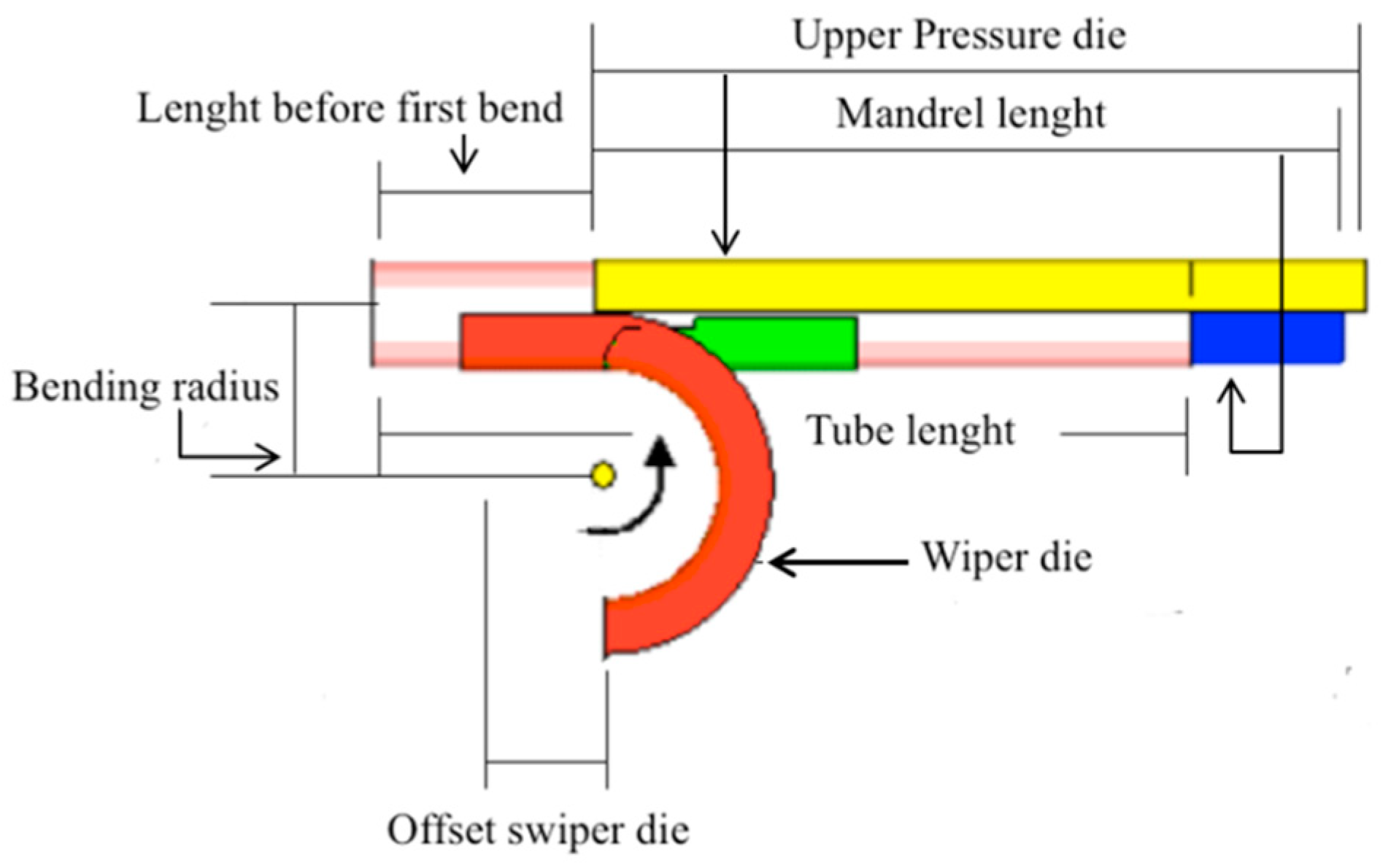
The input related to the shape of tools are described in Figure 1.
The input tools sizes are reported in Table 4.
The other related tools’ geometric parameters are calculated by simulation. Internal spherical elements supporting the bending process (so called balls) are present even if they are not reported in Figure 1. In this paper, four balls with 3.3 mm decreasing diameter sizes are considered. The starting diameter of the first ball is calculated by decreasing the tube diameter by the same measure. It is worth mentioning that an additional support machinery element (called a booster) is not taken into account in the calculations.
The numerical calculation was performed using the Altair HyperWorks™ (2017 version, Troy, MI, USA, commercial software). Such software is able to take into account the material properties reported in Table 3 together with the true stress–true strain steel curves. As far as concerns the tensile material properties, five true stress–true strain curves have been considered, aiming to obtain an average curve. The above materials properties, in particular, are collected in a file readable by the commercial package solver (namely, RADIOSS™). The solver is able to take into account the strain rate by reading the tensile curves performed at different deformation rate conditions. This software allows the adoption of the Hill 48′ yield function. Such a function is known to be ideal for small-sized tubular geometries [45] as a constitutive equation for stainless steel behavior, taking into account the following parameters in order to simulate the bending process:
- bending radius;
- bending angle;
- rotational speed;
- bending temperature.
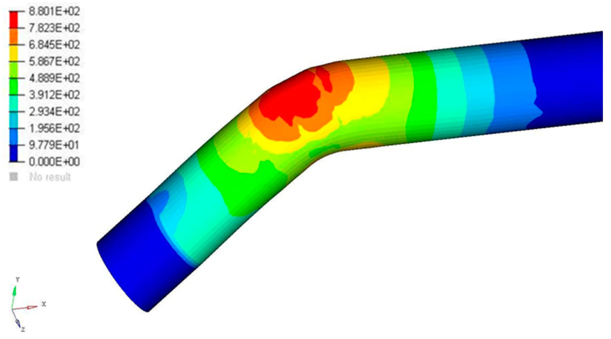
The analysis of the simulation outputs is carried out through mappings of the values calculated by the solver (e.g., internal stress, thinning, and deformation). An example of the obtained maps is reported in Figure 2.
In order to analyze the parameters’ effects on the final process and its feasibility, the maximum stress values obtained on the mappings will be considered in order to consider the critical points of the geometry.
3. Results and Discussion
The effects of the geometric and operational inputs parameters described for the tubes’ plastic deformation are reported below.
3.1. Effect of Tube Diameter
In this section, the effect of the tube’s diameter on the bending process is analyzed, keeping the R/D ratio as a fixed value. R/D = 1 is considered being such a value significative in order to simulate what is commonly performed in the industrial bending process. The tube’s stress behavior as a function of the diameters is reported in Figure 3.
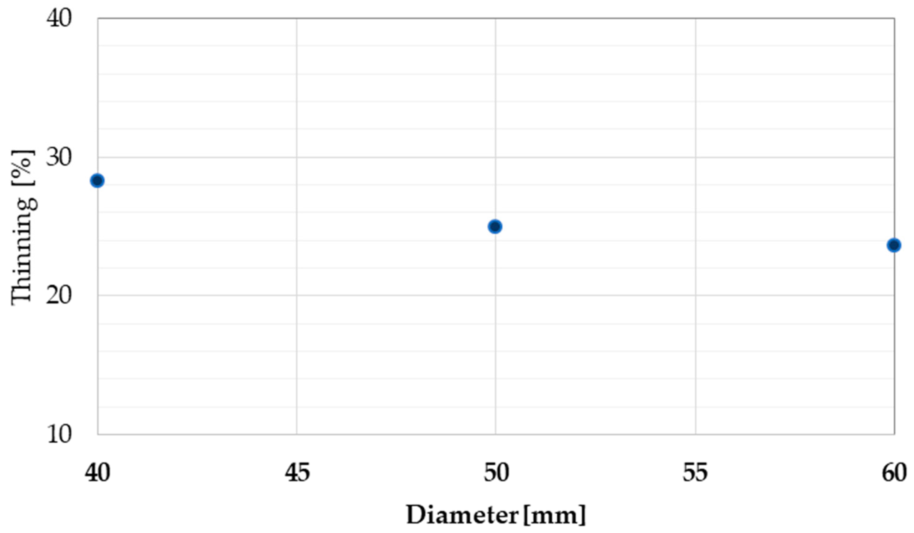
The results allow us to evaluate an effect of about 5% of the tube’s diameter on the internal stress. The same effect is also found for the tube’s thinning (Figure 4). Such results well fit with what is expected from common industrial experience. In addition, they allow us to estimate the stress and thinning loss as a function of the tube’s diameter, thus allowing a process optimization for different tube geometries.
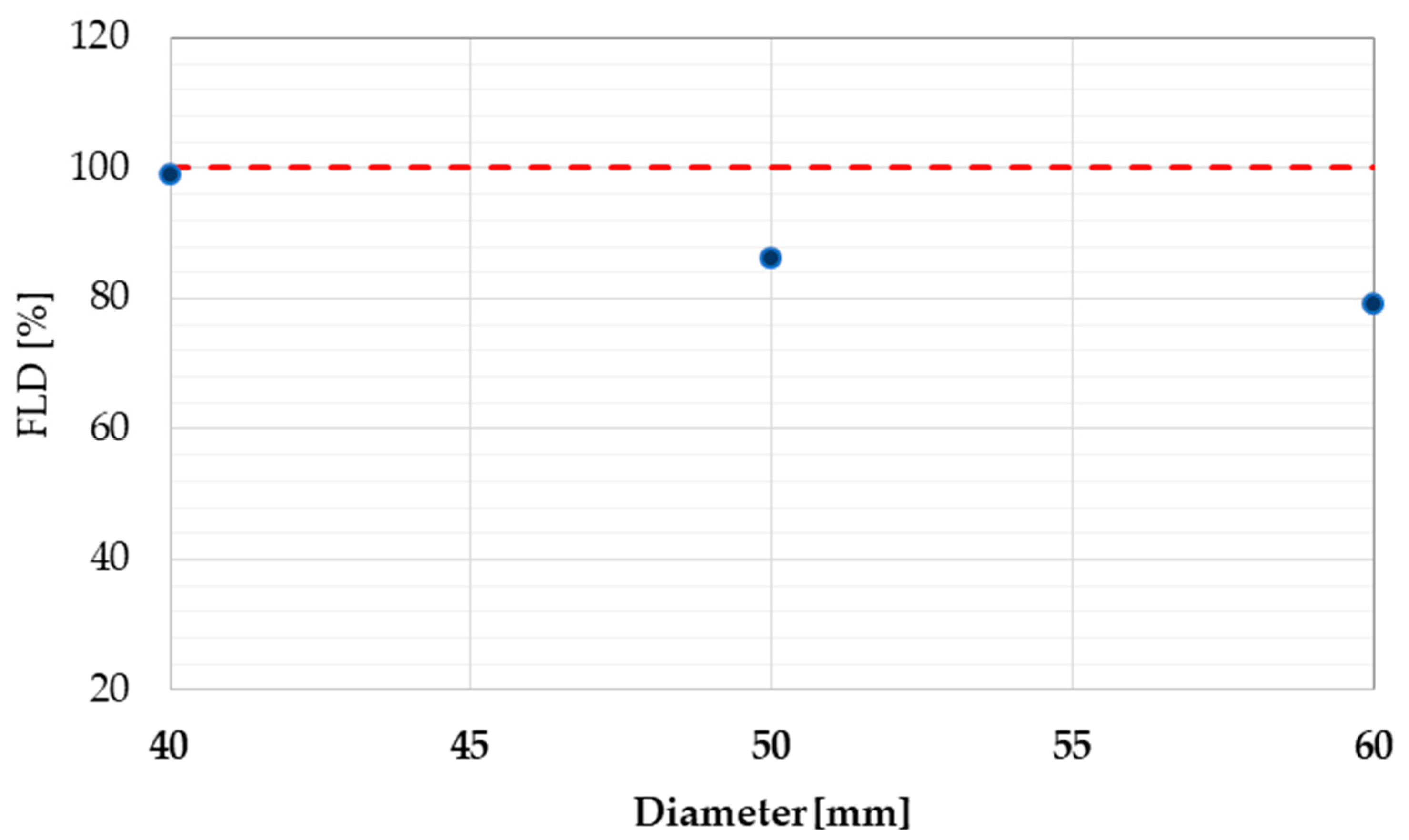
In order to evaluate the deformation capacity and support the above calculation outcomes, the results from FLD diagrams were considered. Figure 5 shows the formability limit (%) as reached during deformation for 441 stainless steel (diameter sizes ranging from 40 to 60 mm). The dashed red line represents the sample breakage. The FLD diagrams confirms that the deformation of the various geometric elements is affected by the diameter size. The results show that an increase in the diameter size will allow a decrease in the breakage risk. Such a result allows us to design the forming process for different pipes sizes, avoiding pipe breakage.
3.2. Tubes Thickness Effect
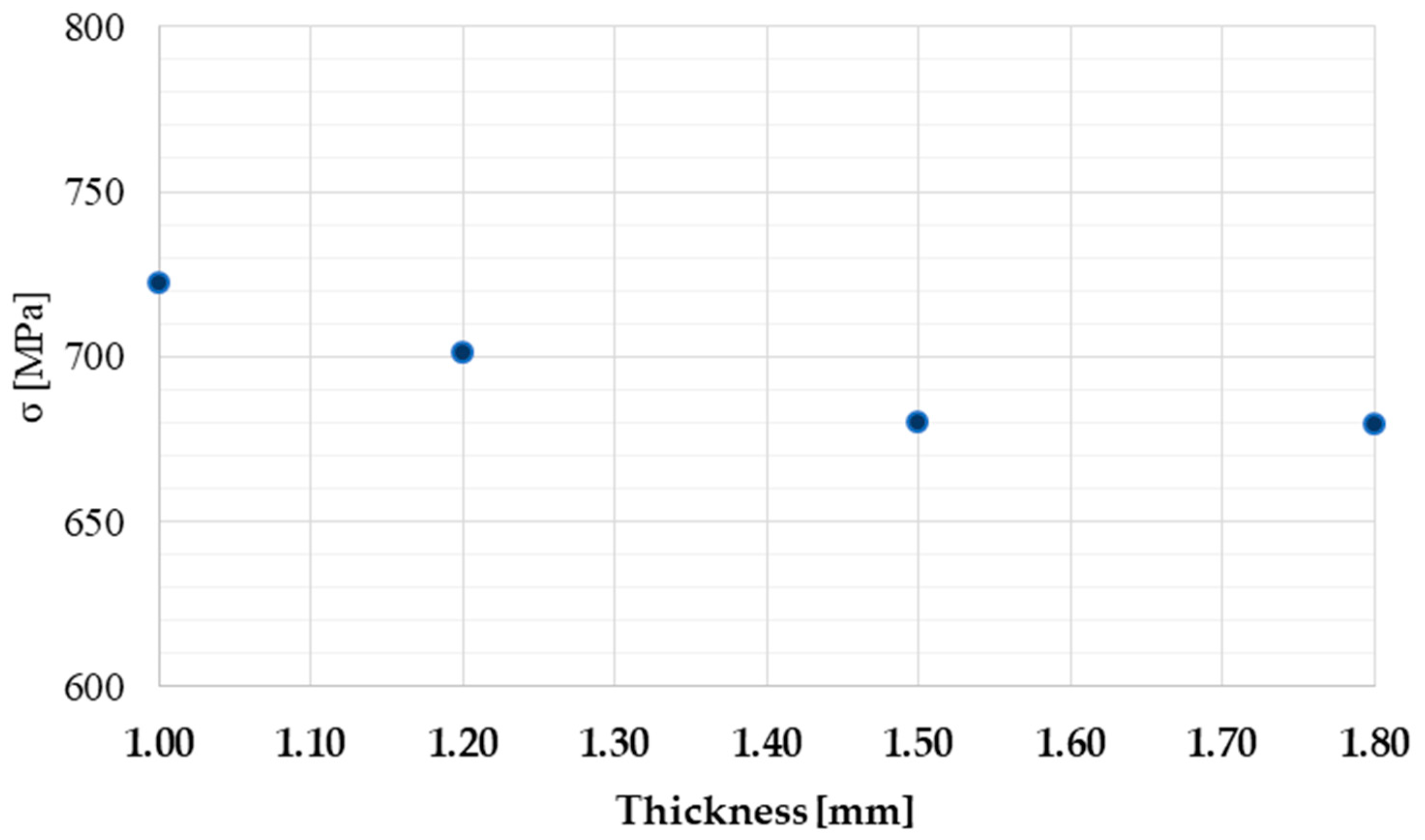
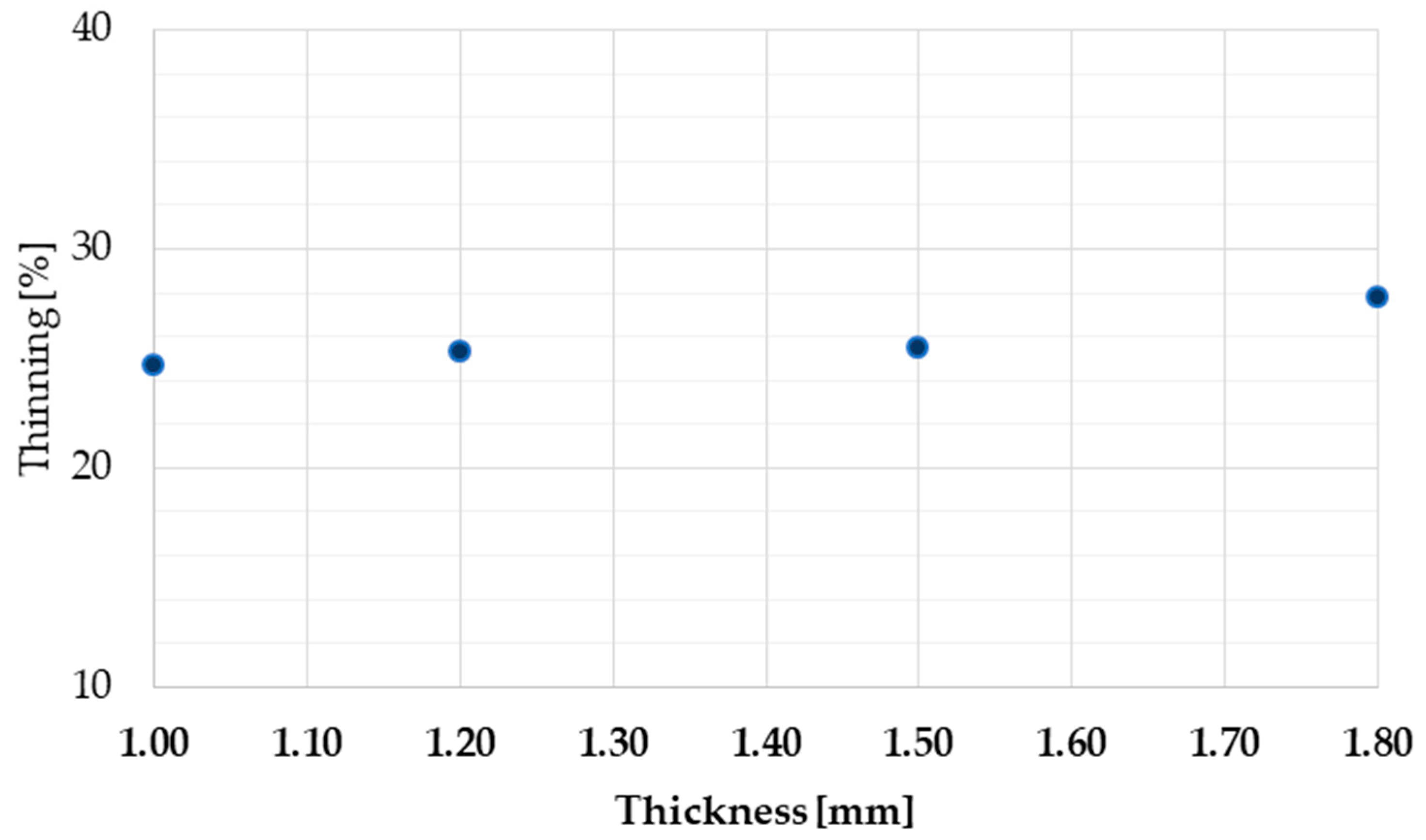
The stress and the tube’s thinning dependence on the thickness are reported in Figure 6 and Figure 7, respectively. The results show that a not-significative stress distribution was found. In particular, the total variation is lower than 2%. On the other hand, the thinning (%) increases as the tube’s thickness increases (Figure 7). Although there have been not relevant variations in terms of stress and thinning, the trend reported in Figure 7 is significant. As a matter of fact, while in the case reported in Section 3.1 the thickness reduction (which is kept constant) has the possibility of being distributed over ever larger diameters, in this case the diameter was fixed as a constant parameter; following that, an increase in thickness led to an increase in the tube’s thinning.
3.3. Speed and Bend Angle Effects
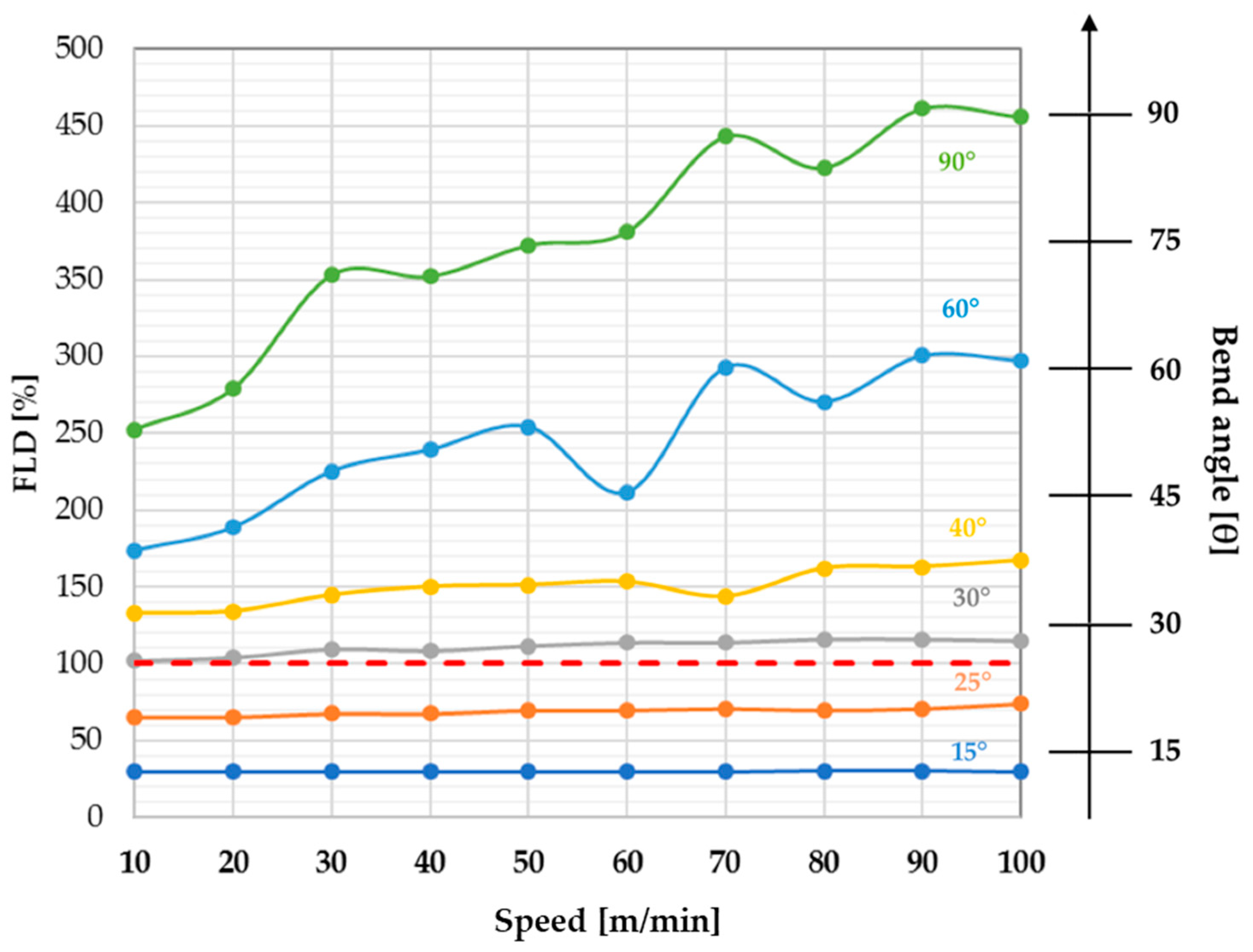
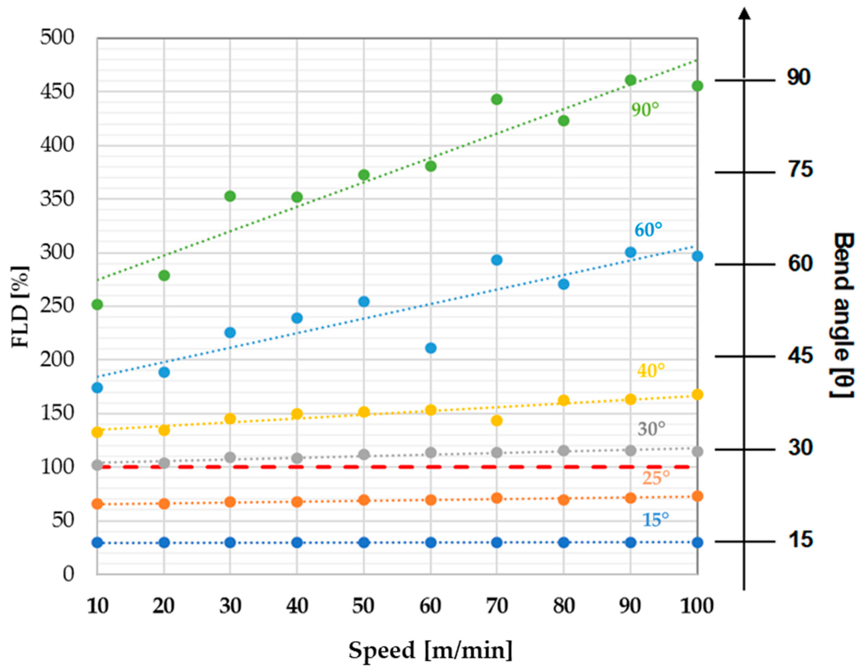
The effect of the speed and bending angle are reported in the following Figure 9.
As far as concerns the speed, the influence of its variation for every bending angle (in the range of 30° and 90° for a common manufacturing process) has been considered. The formability limit (%) for the combination of angle and thickness is shown in Figure 9. In particular, the geometric parameters were fixed, together with the relationship between the diameter and the thickness.
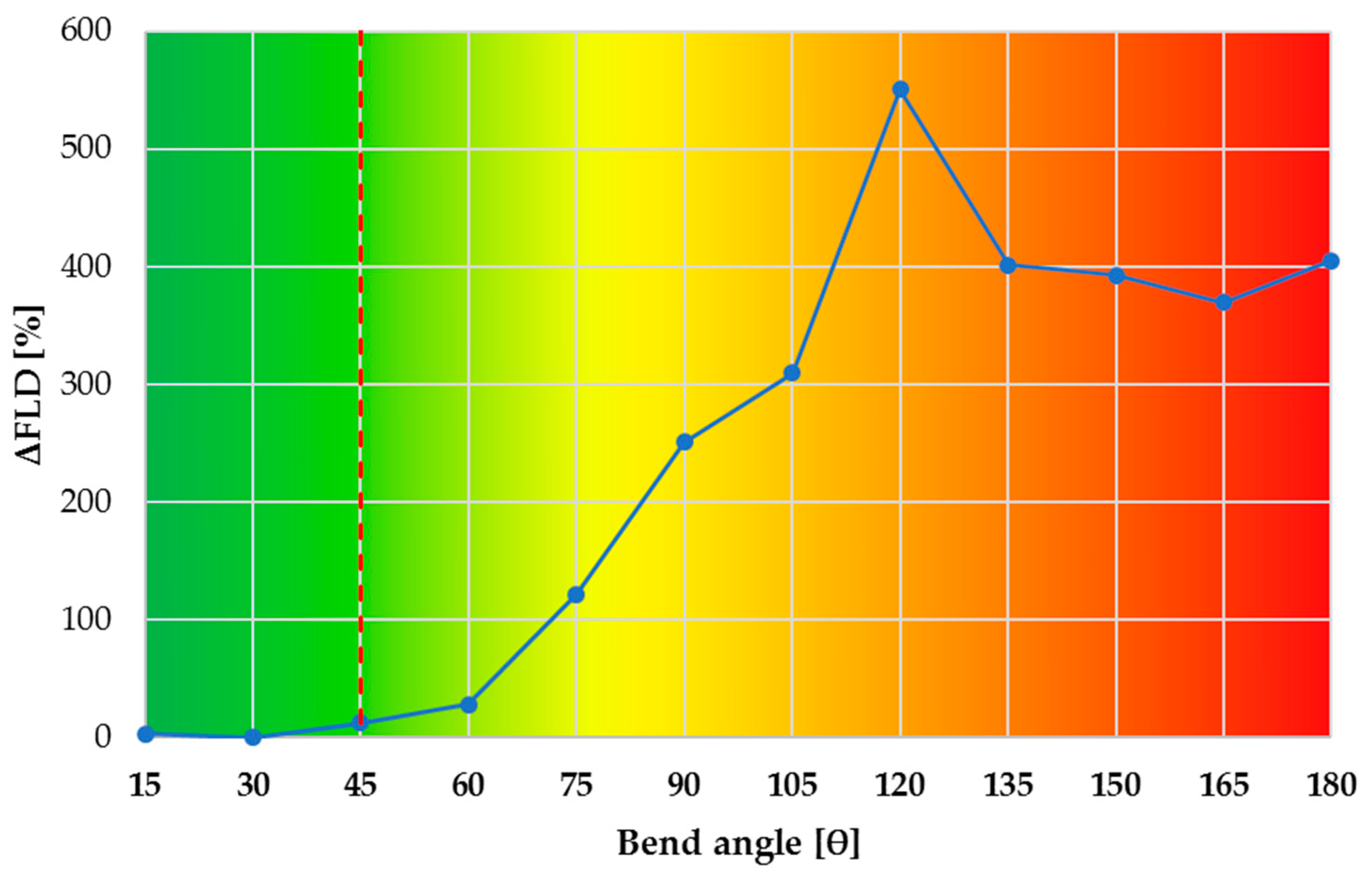
In order to analyze the data, the lines shown in Figure 9 have been interpolated and reported in Figure 10 to better evaluate the influence of the speed. For this reason, the percentage variations between the percentages of formability limits obtained at minimum and maximum feed speeds for each angle, calculated according to Equation (6), are reported in Figure 11.
ΔFLD is closely related to the slope of the interpolated line. Figure 11 shows that in the angle region ranging between 30° and 90° degrees (the most interesting for common industrial processes), the ΔFLD varies almost linearly with respect to the bending angle. If higher angle values are considered the results show that such a parameter reaches a maximum at about 120 degrees of bending, then decreases. The motivations leading to this particular behavior need to be deeply analyzed, but currently we can hypothesize that this is due to the stress concentration being more localized in the first 90° of bending.
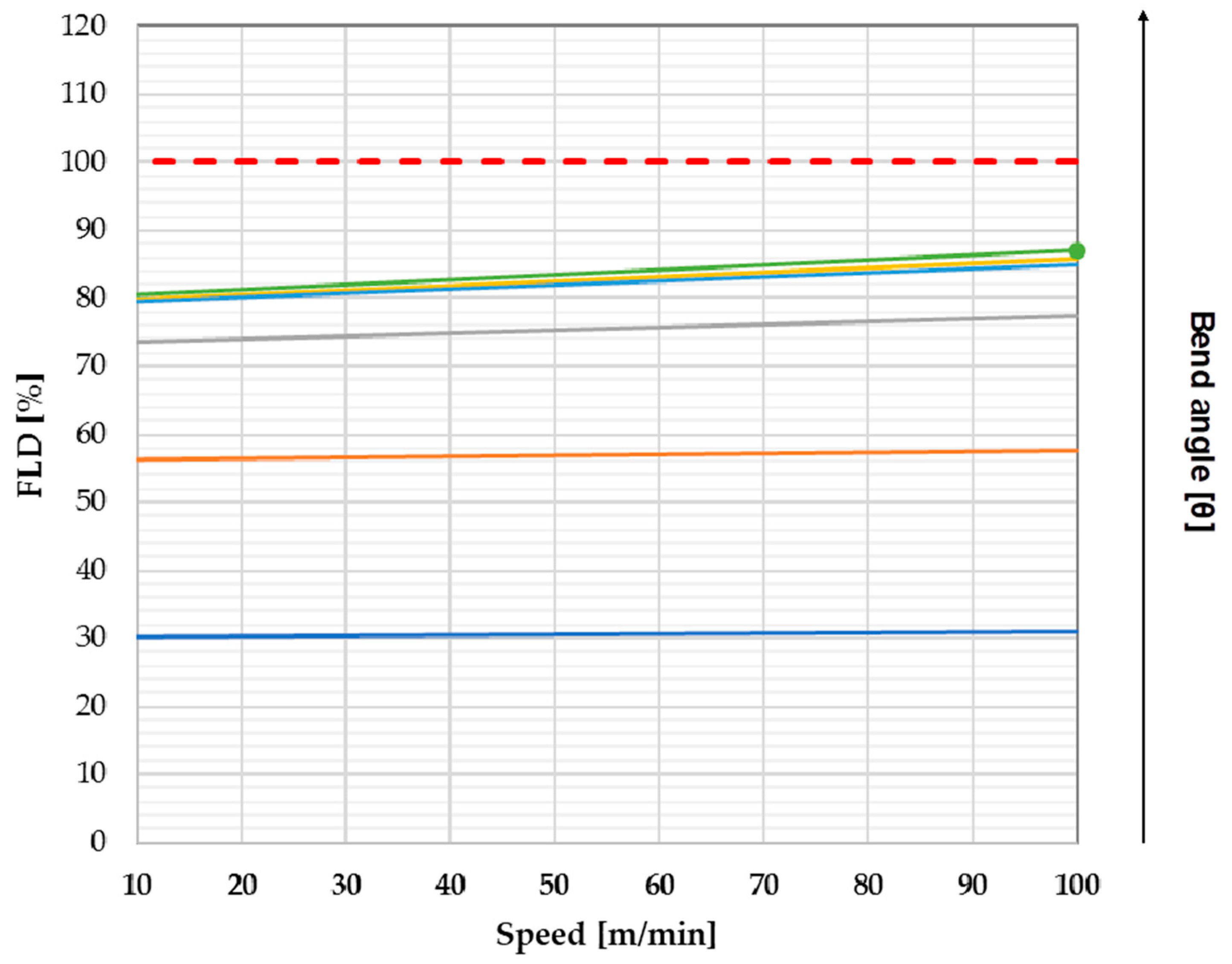
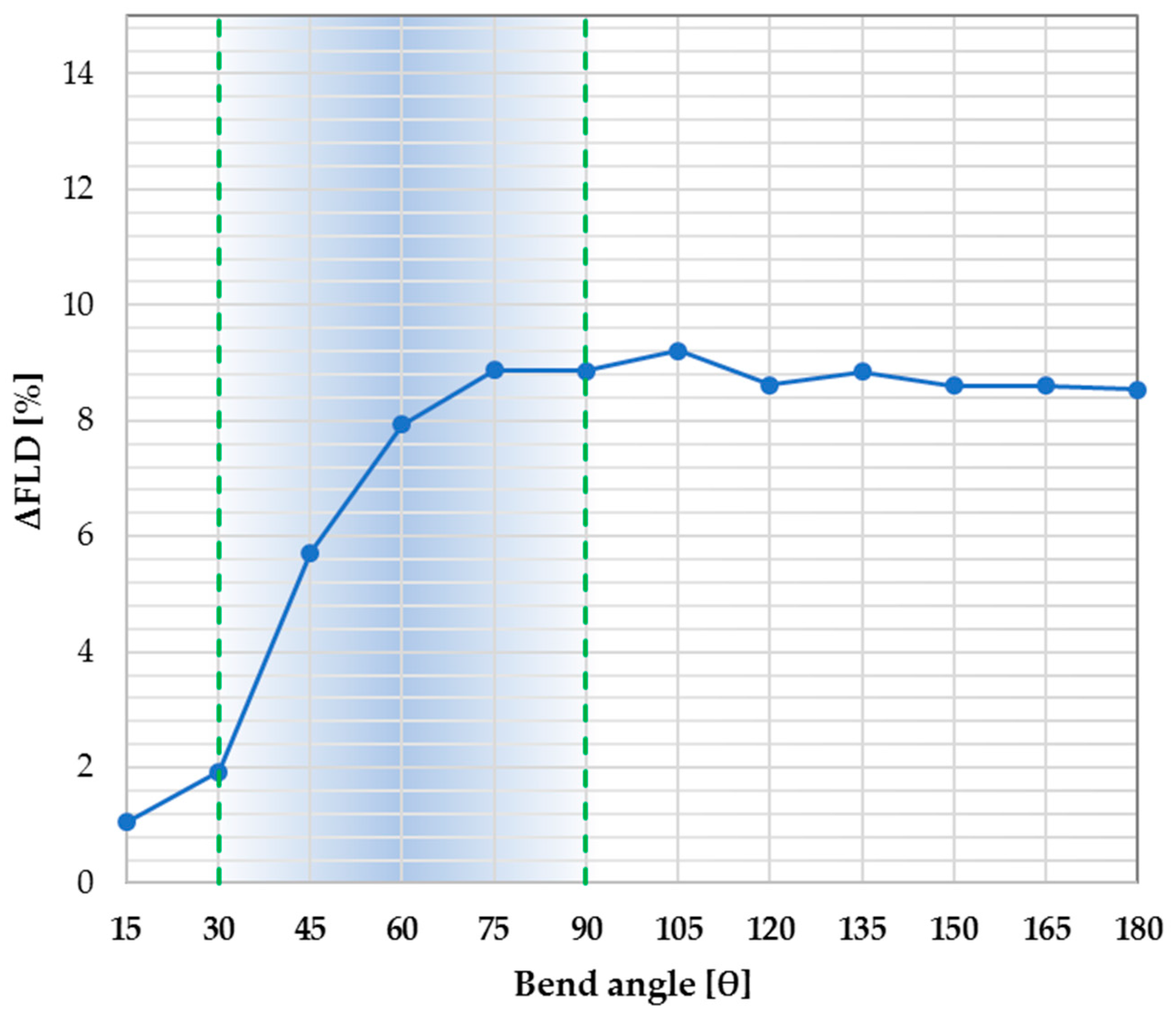
In order to obtain more consistent results, the analysis has been repeated using conditions better reproducing the industrial process. Higher curvature radius values (and the R/D ratio, consequently) were considered. After that, the data were newly interpolated (Figure 12) and the FLD deltas were calculated for the new data set (Figure 13).
Figure 13 shows that the better choice of the R/D ratio leads to an improvement in the sample formability. ΔFLD increases in the bending angle range 30°–90°; it then tends to be stable, keeping away from breaking conditions. Such results suggests that a focus should be put on the R/D ratio on the process. As a matter of fact, this is one of the key issues in the setup of an industrial bending process.
3.4. R/D Effect
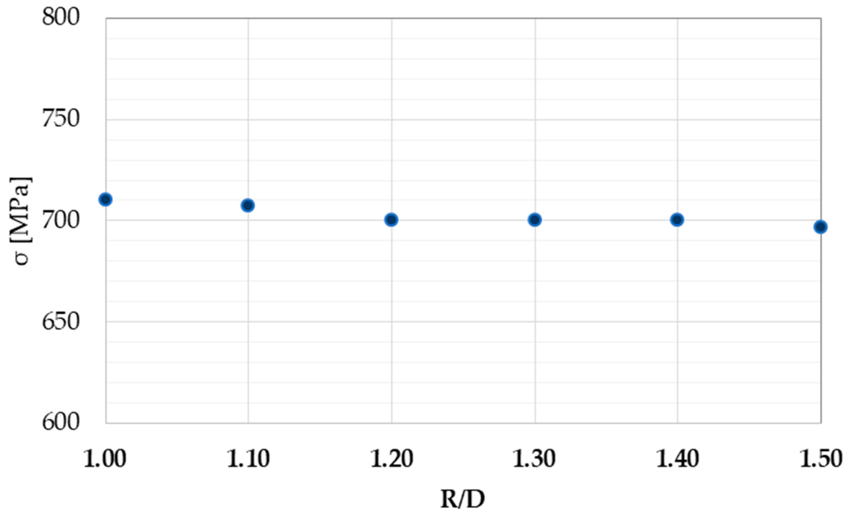
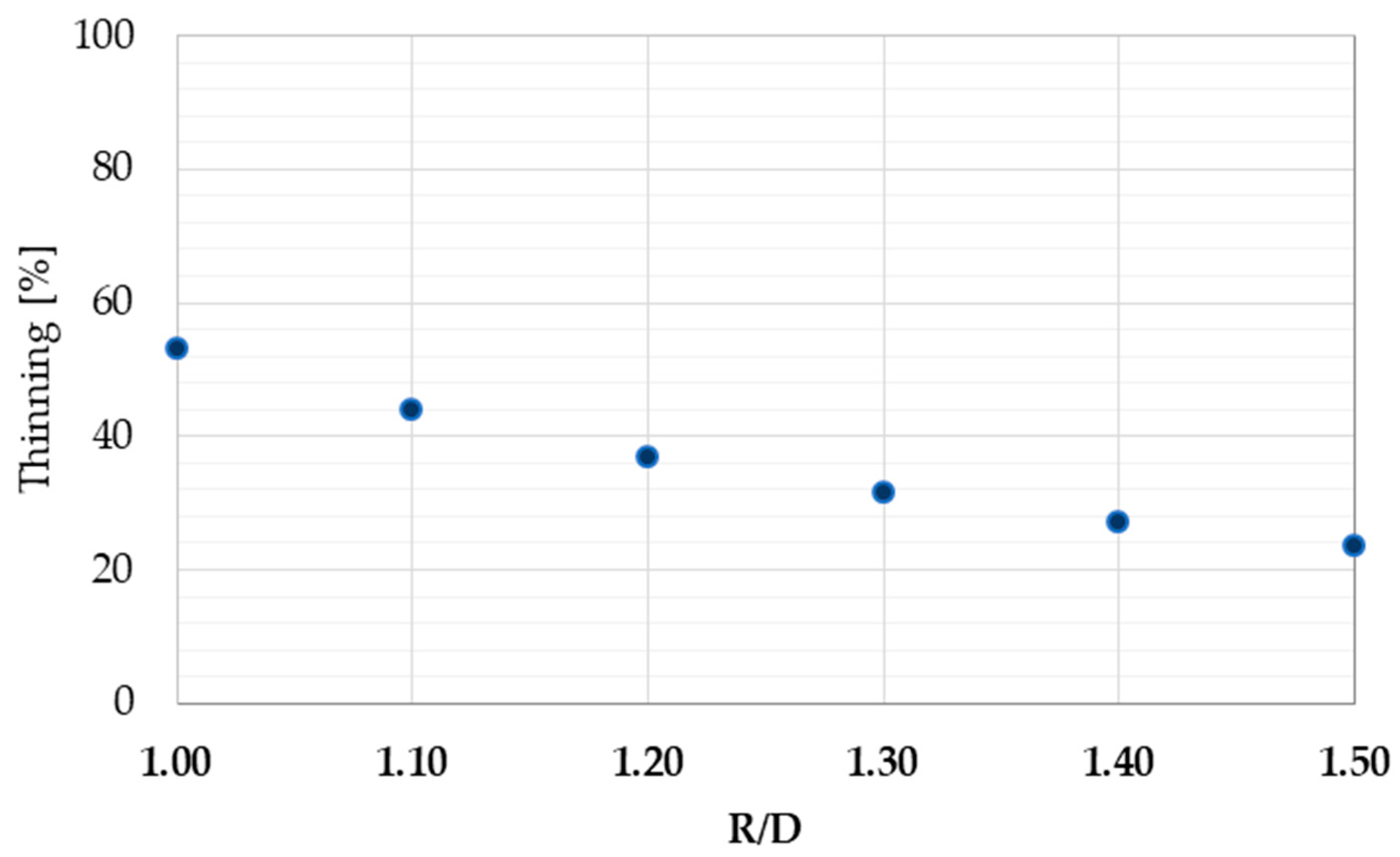
The R/D ratio is commonly adopted as a feasibility index for the bending industrial process. In common industrial practice, this value ranges between 1.0 and 1.5. In fact, R/D < 1 values increase the breakage risk; on the other hand, an R/D > 1.5 is not commonly adopted in the automotive field. The results reported in Figure 14 show a negligible effect of R/D on stresses. On the other hand, a marked R/D ratio effect is found on the tube’s thinning (Figure 15). The results show that the tube’s thinning decreases as the R/D increases. Additionally, in this case the results well fit with what is expected from common industrial experience. In addition, they allow us to estimate the stress and thinning loss as a function of the tubes’ R/D parameter.
3.5. Experimental Validation
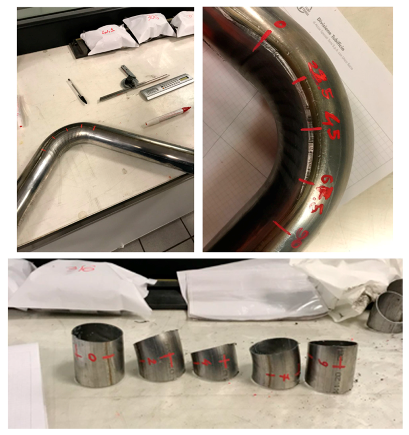
Six samples of 441 steel tubes (50 mm diameter and 1.2 mm thickness size) were considered for validation. All of the considered samples have been chosen with sizes corresponding to the above reported simulations. One of the six samples (for each group) was subjected to tensile tests in order to measure the related stress–strain curve and reduce the uncertainty due to the use of a mean curve. Experimental tests have been carried out according to operational parameters (e.g., rotational velocity and bending radius), as reported in Table 5. The chosen values are those commonly adopted by industries operating in pipe forming for the typical finishing process. Both the thicknesses reached during the bend along the backbone at specific angles, as shown in Figure 16, were measured.
The thickness values were measured for each marked angle, and the average value was considered. The obtained values are shown in Table 6.
The measured thickness variation with the angle and the percentage discrepancy between the measured and calculated thickness as a function of the angle are reported in Table 7. In Table 7, ∆Thickness is defined as the difference between the simulation thickness and the sample mean thickness, as conventionally adopted by companies operating in the tube forming sector.
The deviation of the model from the experimental results (maximum underestimation of 16.36%) corresponds to 67.5 degrees. Such a deviation is probably related to the presence in the experimental tests of an additional support machinery element (the so-called booster), which was not considered in the simulation model. The booster effect in the industrial deformation process is that of pushing the tube during bending in order to avoid the deformations or failure caused by the friction between the element and the machine or by stress concentration. Its action also affects the distribution of the thinning caused by the deformation. As a matter of fact, the tube being pushed by the booster will have more evenly distributed stresses. As a consequence, the deformations and the thinning will take place on a wider area and will not lead to the failure of the piece. Anyway, the accuracy between the modelling and experimental tests is considered good and quite promising, since the discrepancy between the calculated and experimental values is lower than 15% for an angle position lower than 45°. Moreover, the fact that the model appears to underestimate the thickness values allows us to consider its results conservative with respect to the real behavior.
4. Conclusions
This paper analyzes the influence of geometric and operational parameters on the bending process of 441 ferritic stainless steel pipes. Experimental investigations combined with simulations highlighted the effect of each parameter, both operational and geometric, on the final results. The main novelty of the paper is to present an approach able to bridge the gap between fundamental theoretical research and industrial application, putting in evidence the effect of bending process parameters.
Based on the reported results, the following conclusions can be drawn:
- Pipe diameter effect on forming: If the same parameters are considered and the R/D ratio between the radius and diameter is kept constant, an increase in the diameter size (in the typical automotive range) will result in a −9% variation in terms of internal stresses, evaluated according to the von Mises criterion. The thinning of the tube will decrease by −4%, and the feasibility characteristics of the process will improve; in fact, the percentage reaching the formability limit will drop by −20%. The diameter size choice appears therefore to be a key issue in terms of process feasibility. In this sense, the reported approach is a useful tool aimed to properly design, also in quantitative terms, the forming process for different pipe sizes.
- Pipe thickness effect on forming: It is reported that a pipe thickness increase implies more safety for the bending process. In fact, keeping the operating conditions constant, the increase from a thickness of 1.0 mm to a thickness of 1.8 mm will lead to a reduction in the internal stresses of the −6% f, −3% for thinning and −13% in FLD.
- The combined study of bending angle and speed has shown how the simulation has incorrect results when the tube collapses. In non-breaking conditions, the speed has relevant importance in terms of feasibility in the range of the bending angle 30°–90°.
- The simulations show the R/D ratio as the most important parameter in the bending process. An increase in it from 1.0 to 1.5 entails a 30% reduction in thinning and a 60% increase in the bending process success.
The comparison between the calculation and experimental results proved the reported approach to be a useful tool in order to predict and properly design industrial deformation processes. The experimental validation showed a deviation of the model from the experimental case, with a maximum underestimation of 16.36%. Such discrepancy is probably related to the presence in the experimental tests of a booster, which was not included in the simulation model.
Author Contributions
Conceptualization, O.D.P. and R.M.; methodology, O.D.P. and R.M.; formal analysis, O.D.P., G.N., and M.G.; paper preparation, O.D.P. and A.D.S.; supervision, R.M. and A.D.S. All authors have read and agreed to the published version of the manuscript.
Funding
This research received no external funding.
Conflicts of Interest
The authors declare no conflict of interest.
References
- Marshall, P. Austenitic Stainless Steels: Microstructure and Mechanical Properties; Elsevier Applied Science Publisher: Amsterdam, The Netherlands, 1984. [Google Scholar]
- Di Schino, A. Manufacturing and application of stainless steels. Metals 2020, 10, 327. [Google Scholar] [CrossRef] [Green Version]
- Liu, W.; Lian, J.; Munstermann, S.; Zeng, C.; Fang, X. Prediction of crack formation in the progressive folding of square tubes during dynamic axial crushing. Int. J. Mech. Sci. 2020, 176, 105534. [Google Scholar] [CrossRef]
- Corradi, M.; Osofero, A.I.; Borri, A. Repair and Reinforcement of Historic Timber Structures with Stainless Steel—A Review. Metals 2019, 9, 106. [Google Scholar] [CrossRef] [Green Version]
- Gedge, G. Structural uses of stainless steel—Buildings and civil engineering. J. Constr. Steel Res. 2008, 64, 1194–1198. [Google Scholar] [CrossRef]
- Di Schino, A. Analysis of heat treatment effect on microstructural features evolution in a micro-alloyed martensitic steel. Acta Met. Slovaca 2016, 22, 266–270. [Google Scholar] [CrossRef] [Green Version]
- Sharma, D.K.; Filipponi, M.; Di Schino, A.; Rossi, F.; Castaldi, J. Corrosion behavior of high temperature fuel cells: Issues for materials selection. Metalurgija 2019, 58, 347–351. [Google Scholar]
- Gennari, C.; Lago, M.; Bogre, B.; Meszaros, I.; Calliari, I.; Pezzato, L. Microstructural and corrosion properties of cold rolled laser welded UNS S32750 duplex stainless steel. Metals 2018, 8, 1074. [Google Scholar] [CrossRef] [Green Version]
- Fava, A.; Montanari, R.; Varone, A. Mechanical spectroscopy investigation of point defect-driven phenomena in a Chromium martensitic steel. Metals 2018, 8, 870. [Google Scholar] [CrossRef] [Green Version]
- Di Schino, A.; Kenny, J.M.; Abbruzzese, G. Analysis of the recrystallization and grain growth processes in AISI 316 stainless steel. J. Mat. Sci. 2002, 37, 5291–5298. [Google Scholar] [CrossRef]
- Di Schino, A.; Testani, C. Corrosion behavior and mechanical properties of AISI 316 stainless steel clad Q235 plate. Metals 2020, 10, 552. [Google Scholar] [CrossRef]
- Rufini, R.; Di Pietro, O.; Di Schino, A. Predictive simulation of plastic processing of welded stainless steel pipes. Metals 2018, 8, 519. [Google Scholar] [CrossRef] [Green Version]
- Di Schino, A.; Valentini, L.; Kenny, J.M.; Gerbig, Y.; Ahmed, I.; Hefke, H. Wear resistance of high-nitrogen austenitic stainless steel coated with nitrogenated amorphous carbon films. Surf. Coat. Technol. 2002, 161, 224–231. [Google Scholar] [CrossRef]
- Di Schino, A.; Di Nunzio, P.E.; Turconi, G.L. Microstructure evolution during tempering of martensite in medium carbon steel. Mater. Sci. Forum 2007, 558, 1435–1441. [Google Scholar]
- Di Schino, A.; Alleva, L.; Guagnelli, M. Microstructure evolution during quenching and tempering of martensite in a medium C steel. Mater. Sci. Forum 2012, 715–716, 860–865. [Google Scholar]
- Zitelli, C.; Folgarait, P.; Di Schino, A. Laser powder bed fusion of stainless steel grades: A review. Metals 2019, 9, 731. [Google Scholar] [CrossRef] [Green Version]
- Mancini, S.; Langellotto, L.; Di Nunzio, P.E.; Zitelli, C.; Di Schino, A. Defect reduction and quality optimisation by modelling plastic deformation and metallurgical evolution in ferritic stainless steels. Metals 2020, 10, 186. [Google Scholar] [CrossRef] [Green Version]
- Gardner, L. The use of stainless steel in structures. Prog. Struct. Eng. Mat. 2005, 7, 45–55. [Google Scholar] [CrossRef]
- Mulidran, P.; Siser, M.; Slota, J.; Spisak, E.; Sleziak, T. Numerical Prediction of Forming Car Body Parts with Emphasis on Springback. Metals 2018, 8, 60435. [Google Scholar] [CrossRef] [Green Version]
- Mei, Z.; Khun, G.; He, Y. Advances and trends in plastic forming technologies for welded tubes. Chin. J. Aeron. 2016, 29, 305–315. [Google Scholar]
- Oliveira, M.C.; Fernandes, J.B. Modelling and simulation of sheet metals forming processes. Metals 2019, 9, 1356. [Google Scholar] [CrossRef] [Green Version]
- Cherouat, A.; Borouchaki, H.; Zhang, J. Simulation of Sheet Metal Forming Processes Using a Fully Rheological-Damage Constitutive Model Coupling and a Specific 3D Remeshing Method. Metals 2018, 8, 991. [Google Scholar] [CrossRef] [Green Version]
- Bong, H.J.; Barlat, F.; Lee, M.; Ahn, D.C. The forming limit diagram of ferritic stainless steel sheets: Experiments and modeling. Int. J. Mech. Sci. 2012, 64, 1–10. [Google Scholar] [CrossRef]
- Zhang, H.; Liu, Y. The inverse parameter identification of Hill’48 yield function for small-sized tube combining response surface methodology and three-point bending. J. Mat. Res. 2017, 32, 2343–2351. [Google Scholar] [CrossRef]
- Lehmberg, A.; Suderkoetter, C.; Glaesner, T.; Brokmeier, H.G. Forming behavior of stainless steel sheets at different material thicknesses. Mater. Sci. Eng. 2019, 651, 012082. [Google Scholar]
- Scott, T.; Kotadia, H. Microstructural evolution of 316L austenitic stainless steel during in-situ biaxial deformation and annealing. Mat. Chat. 2020, 163, 110288. [Google Scholar]
- He, Y.; Heng, L.; Zhiyoing, Z.; Mei, Z.; Jing, L.; Guangjun, L. Advances and Trends on Tube Bending Forming Technologies. Chin. J. Aeron. 2012, 25, 1–12. [Google Scholar]
- Wu, W.Y.; Zhang, P.; Zeng, X.Q.; Li, J.; Yao, S.S.; Luo, A.A. Bendability tubes using a rotary draw bender. Mater. Sci. Eng. A 2008, 486, 596–601. [Google Scholar] [CrossRef]
- Liu, K.X.; Liu, Y.L.; Yang, H.; Zhao, G.Y. Experimental study on cross-section distortion of thin-walled rectangular tube by rotary draw bending. Int. J. Mater. Prod. Technol. 2011, 42, 110–120. [Google Scholar] [CrossRef]
- Liu, K.X.; Liu, Y.L.; Yang, H. Experimental study on the effect of dies on wall thickness distribution in NC bending of thin-walled rectangular tube. Int. J. Mater. Prod. Technol. 2013, 68, 1867–1874. [Google Scholar]
- Tang, N. Plastic-deformation analysis in tube bending. Int. J. Pres. Vessels. Pip. 2000, 77, 751–759. [Google Scholar] [CrossRef]
- Al-Qureshi, H.; Russo, A. Spring-back and residual stresses in bending of thin-walled tubes. Mater. Des. 2002, 23, 217–222. [Google Scholar] [CrossRef]
- Chen, J.; Ding, J.; Bai, X. In-plane strain solution of stress and defects of tube bending with exponential hardening law. Mech. Based Des. Struct. Mach. Int. J. 2012, 40, 257–276. [Google Scholar]
- Li, H.; Yang, H.; Song, F.F.; Zhan, M.; Li, G.J. Spring-back characterization and behaviors of high-strength tube in cold rotary draw bending. J. Mater. Process. Technol. 2012, 212, 1973–1987. [Google Scholar] [CrossRef]
- Jeong, H.S.; Ha, M.Y.; Cho, J.R. Theoretical and FE analysis for fine tube bending to predict spring-back. Int. J. Precis. Eng. Manuf. 2012, 13, 2143–2148. [Google Scholar] [CrossRef]
- Liu, J.; Tang, C.; Ning, R. Deformation calculation of cross section based on virtual force in thin-walled tube bending process. Chin. J. Mech. Eng. 2009, 22, 696–701. [Google Scholar] [CrossRef]
- Li, H.; Yang, H.; Yan, J.; Zhan, M. Numerical study on deformation behaviors of thin-walled tube NC bending with large diameter and small bending radius. Comput. Mat. Sci. 2009, 45, 921–934. [Google Scholar] [CrossRef]
- Napoli, G.; Di Schino, A.; Paura, M.; Vela, T. Colouring titanium alloys by anodic oxidation. Metalurgija 2018, 57, 111–113. [Google Scholar]
- Di Schino, A.; Di Nunzio, P. Metallurgical aspects related to contact fatigue phenomena in steels for back up rolling. Acta Metall. Slovaca 2017, 23, 62–71. [Google Scholar] [CrossRef] [Green Version]
- Di Schino, A. Analysis of phase transformation in high strength low alloyed steels. Metalurgija 2017, 56, 349–352. [Google Scholar]
- Wang, S.; Wei, K.; Li, J.; Liu, Y.; Huang, Z.; Mao, Q.; Li, Y. Enhanced tensile properties of 316L stainless steel processed by a novel ultrasonic resonance plastic deformation technique. Mater. Lett. 2019, 236, 342–345. [Google Scholar] [CrossRef]
- Kaushal, M.; Joshi, Y.M. Three-dimensional yielding in anisotropic materials: Validation of Hill’s criterion. Soft Matter 2019, 15, 4915–4920. [Google Scholar] [CrossRef] [PubMed]
- Cazacu, O.; Revil-Baudard, B.; Chandola, N. Yield criteria for anisotropic polycrystals. In Plasticity-Damage Couplings: From Single Crystal to Polycrystalline Materials. Solid Mechanics and Its Applications; Springer International Publishing: Cham, Switzerland, 2019; volume 253. [Google Scholar]
- Lumelskyj, D.; Rojek, J.; Tkocz, M. Numerical simulations of Nakazima formability tests with prediction of failure. Appl. Mech. 2015, 60, 184–194. [Google Scholar]
- Yang, T.B.; Yu, Z.Q.; Xu, C.B.; Li, S.H. Numerical analysis for forming limit of welded tube in hydroforming. J. Shanghai Jiaotong Univ. 2011, 45, 6–10. [Google Scholar]
Figure 1.
Tools for the bending simulation.

Figure 2.
Stress mapping on bent tube.

Figure 3.
Mean maximum stress behavior as a function of diameter size for 441 steel with a 1.5 mm thickness.
Figure 3.
Mean maximum stress behavior as a function of diameter size for 441 steel with a 1.5 mm thickness.

Figure 4.
Maximum thinning as a function of the diameter size for 441 steel with a 1.5 mm thickness.
Figure 4.
Maximum thinning as a function of the diameter size for 441 steel with a 1.5 mm thickness.

Figure 5.
Formability limit (%) as a function of the tube’s diameter for 441 with a 1.5 mm thickness.
Figure 5.
Formability limit (%) as a function of the tube’s diameter for 441 with a 1.5 mm thickness.

Figure 6.
Mean maximum stress behavior as a function of thickness for 441 steel with a 50 mm diameter.
Figure 6.
Mean maximum stress behavior as a function of thickness for 441 steel with a 50 mm diameter.

Figure 7.
Maximum thinning as a function of thickness size for 441 steel with a 50 mm diameter.

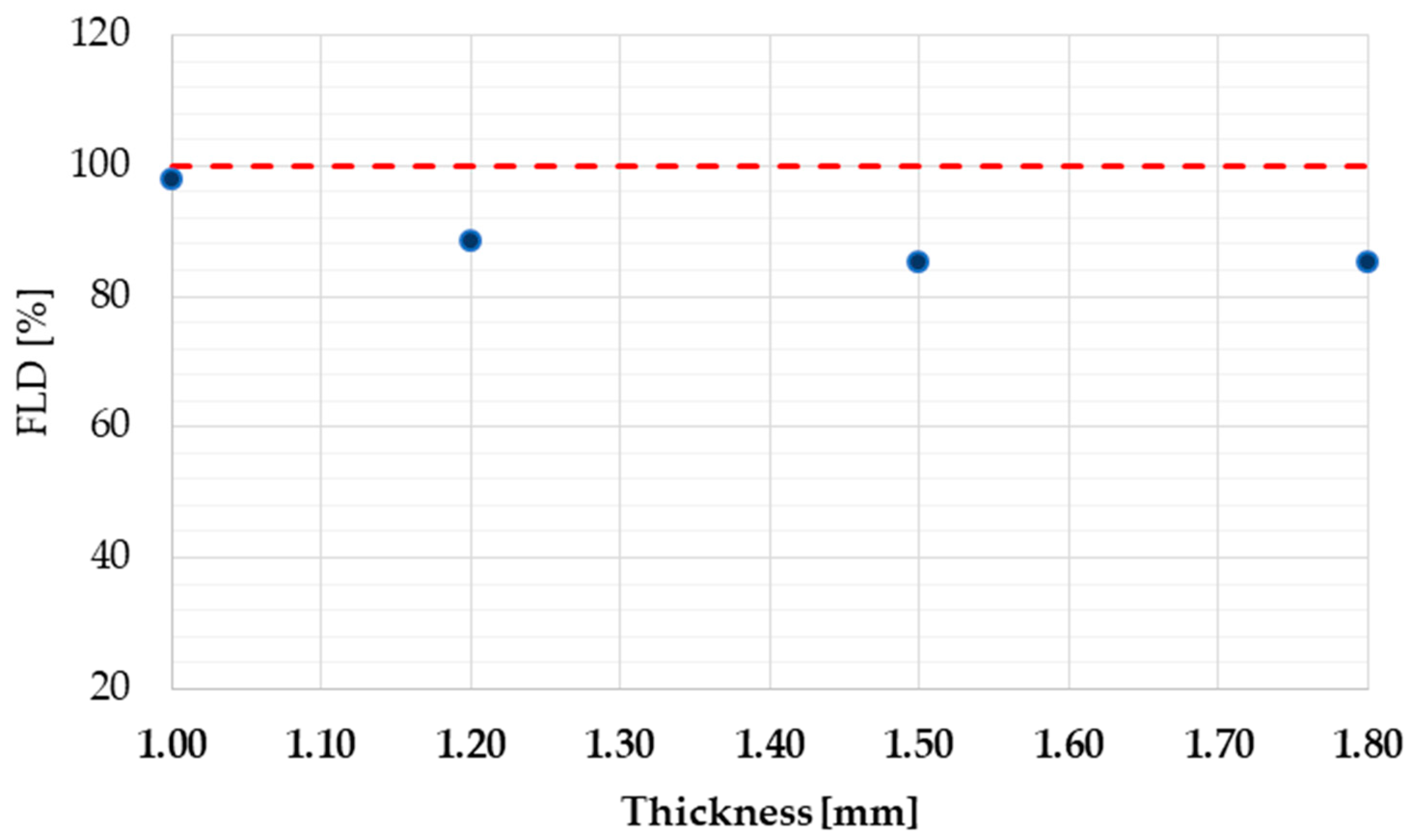
Figure 8.
Formability limit (%) as a function of the thickness for 441 with a 50 mm diameter.

Figure 9.
A 2D plot of the formability limit (%) for different speed and angle combinations.

Figure 10.
Formability Limit Diagram (FLD) dependence on speed for different bending angles (linear interpolation).
Figure 10.
Formability Limit Diagram (FLD) dependence on speed for different bending angles (linear interpolation).

Figure 11.
Goodness of the simulation output beyond the breaking of the worked piece (red dotted line).
Figure 11.
Goodness of the simulation output beyond the breaking of the worked piece (red dotted line).

Figure 12.
Linear interpolation of the formability limit (%) for each combination of speed and angle.
Figure 12.
Linear interpolation of the formability limit (%) for each combination of speed and angle.

Figure 13.
FLD dependence on the bending angle.

Figure 14.
Maximum equivalent stress dependence on the R/D ratio.

Figure 15.
Maximum thinning dependence on the R/D ratio.

Figure 16.
Thickness measuring grid on the backbone.


Table 1.
Chemical analysis of 441 (main elements, mass. %).
| Steel Grade | C | Cr | Ni | Mo | Ti+Nb | Fe |
|---|---|---|---|---|---|---|
| 441 | 0.02–0.04 | 17.5–18.5 | − | − | 0.55% | Balance |
Table 2.
Materials selected for the simulations with their geometric characteristics.
| Steel Grade | Tube Diameter [mm] | Tube Thickness [mm] |
|---|---|---|
| 441 | 40; 45; 50; 55; 60 | 1.0; 1.2; 1.5; 1.8 |
Table 3.
Steel properties [2].
Table 3.
Steel properties [2].
| Density | Young Modulus | Poisson Ratio | Lankford Value | Strain Hardening |
|---|---|---|---|---|
| 210,000.0 | 0.30 | 1.30–1.40 | 0.20–0.25 |
Table 4.
Adopted bending tool sizes.
| Mandrel [mm] | Upper Pressure Die [mm] | Offset Swiper Die [mm] | Bending Radius [mm] |
|---|---|---|---|
| 750 | 750 | 100 | 100 |
Table 5.
Testing conditions.
| Rotational Velocity [rad/sec] | Bending Radius [mm] | Temperature [°C] | Bend Angle [ϑ] |
|---|---|---|---|
| 1.6235 | 100.0 | 25.0 | 90 |
Table 6.
Thickness for the 441 steel samples as measured at different considered angles (mm).
| Angle | Thickness (mm) | ||||||
|---|---|---|---|---|---|---|---|
| Specimen n° 1 | Specimen n° 2 | Specimen n° 3 | Specimen n° 4 | Specimen n° 5 | Specimen n° 6 | MeanValue | |
| 0° | 1.169 | 1.200 | 1.180 | 1.124 | 1.250 | 1.235 | 1.193 |
| 22.5° | 1.003 | 1.019 | 1.026 | 1.023 | 1.123 | 1.101 | 1.049 |
| 45° | 0.982 | 0.993 | 1.002 | 1.058 | 1.157 | 1.016 | 1.035 |
| 67.5° | 1.086 | 1.016 | 1.050 | 1.029 | 1.166 | 1.052 | 1.067 |
| 90° | 1.200 | 1.180 | 1.180 | 1.152 | 1.149 | 1.161 | 1.166 |
Table 7.
Comparison between the calculated and measured thickness at different angles.
| Measurement Angle | Simulation Thickness [mm] | Sample Mean Thickness [mm] | ∆Thickness [mm] | Percentage Variation [%] |
|---|---|---|---|---|
| 0° | 1.168 | 1.193 | −0.025 | −2.10 |
| 22.5° | 1.014 | 1.049 | −0.035 | −3.35 |
| 45° | 0.876 | 1.035 | −0.159 | −15.34 |
| 67.5° | 0.892 | 1.067 | −0.175 | −16.36 |
| 90° | 1.171 | 1.170 | 0.001 | 0.06 |
© 2020 by the authors. Licensee MDPI, Basel, Switzerland. This article is an open access article distributed under the terms and conditions of the Creative Commons Attribution (CC BY) license (http://creativecommons.org/licenses/by/4.0/).
Share and Cite
MDPI and ACS Style
Di Pietro, O.; Napoli, G.; Gaggiotti, M.; Marini, R.; Di Schino, A. Analysis of Forming Parameters Involved in Plastic Deformation of 441 Ferritic Stainless Steel Tubes. Metals 2020, 10, 1013. https://doi.org/10.3390/met10081013
AMA Style
Di Pietro O, Napoli G, Gaggiotti M, Marini R, Di Schino A. Analysis of Forming Parameters Involved in Plastic Deformation of 441 Ferritic Stainless Steel Tubes. Metals. 2020; 10(8):1013. https://doi.org/10.3390/met10081013
Chicago/Turabian StyleDi Pietro, Orlando, Giuseppe Napoli, Matteo Gaggiotti, Roberto Marini, and Andrea Di Schino. 2020. "Analysis of Forming Parameters Involved in Plastic Deformation of 441 Ferritic Stainless Steel Tubes" Metals 10, no. 8: 1013. https://doi.org/10.3390/met10081013
Note that from the first issue of 2016, this journal uses article numbers instead of page numbers. See further details here.