An Improved Moth-Flame Optimization Algorithm for Engineering Problems


1
Institute of Management Science and Engineering, and School of Business, Henan University, Kaifeng 475004, China
2
School of Business, Henan University, Kaifeng 475004, China
3
Institute of Intelligent Network Systems, and Software School, Henan University, Kaifeng 475004, China
*
Author to whom correspondence should be addressed.
Symmetry 2020, 12(8), 1234; https://doi.org/10.3390/sym12081234
Submission received: 22 June 2020
/
Revised: 19 July 2020
/
Accepted: 20 July 2020
/
Published: 27 July 2020
Abstract
:In this paper, an improved moth-flame optimization algorithm (IMFO) is presented to solve engineering problems. Two novel effective strategies composed of Lévy flight and dimension-by-dimension evaluation are synchronously introduced into the moth-flame optimization algorithm (MFO) to maintain a great global exploration ability and effective balance between the global and local search. The search strategy of Lévy flight is used as a regulator of the moth-position update mechanism of global search to maintain a good research population diversity and expand the algorithm’s global search capability, and the dimension-by-dimension evaluation mechanism is added, which can effectively improve the quality of the solution and balance the global search and local development capability. To substantiate the efficacy of the enhanced algorithm, the proposed algorithm is then tested on a set of 23 benchmark test functions. It is also used to solve four classical engineering design problems, with great progress. In terms of test functions, the experimental results and analysis show that the proposed method is effective and better than other well-known nature-inspired algorithms in terms of convergence speed and accuracy. Additionally, the results of the solution of the engineering problems demonstrate the merits of this algorithm in solving challenging problems with constrained and unknown search spaces.
1. Introduction
The moth-flame optimization algorithm [1] was recently proposed by Mirjalili in 2015, which is one of the latest algorithms that has gained extensive attention in recent years. This new intelligent algorithm is based on the biological behavior of moths fighting flames in nature. Its biological principle is the moth’s night flight mechanism. The moth updates its position by spiraling around the flame. The moth-flame optimization algorithm (MFO) algorithm has the advantages of having few setting parameters, being easy to understand and implement, and having fast convergence. Nevertheless, we can see from the literature that there is still room for improvement in the moth-flame optimization algorithm. Therefore, in the past two years, many scholars have tried to improve the algorithm in different aspects. Furthermore, the algorithm is widely used in physics, medicine, economics and other fields. Eventually, many scholars have put forward examples about the application of the algorithm in different fields to solve practical problems.
The moth-flame optimization algorithm is widely used in the field of physics; the related research is as follows. Hitarth Buch [2] proposed an improved adaptive moth-flame optimization algorithm, which was effectively used to solve the optimal power flow problem. Avishek Das [3] used the moth-flame optimization algorithm to determine the optimal set of current excitation weights and determine the optimal spacing between array elements in the three-ring structure of the improved concentric antenna array (CCAA). Satomi Ishiguro [4] proposed a new method to optimize the loading mode of nuclear reactors—a multi-group moth-flame optimization algorithm with predators. Hegazy Rezk [5] studied the hybrid moth-flame optimization algorithm and the power condition of the maximum solar photovoltaic/hot spot system with incremental conductance tracking under different conditions. Mahrous a. Taher [6] used an improved moth-flame optimization algorithm to solve the optimal power flow problem. Mohamed a. Tolba [7] proposed the moth-flame optimization algorithm to solve the problem of the optimal configuration of a distributed power supply and shunt capacitor banks, in which it played a substantial role in improving voltage distribution and voltage stability, improving the power quality of the system and reducing the power loss of the system. Indrajit N. Trivedi [8] used the moth-flame optimizer to optimize the power flow of a power system to improve voltage stability and reduce losses.
The moth-flame optimization algorithm has also been applied to the medical and other relevant fields. Some scholars’ studies are as follows. Gehad Ismail Sayed [9] used neutrophils to optimize the moth-flame population for the automatic detection of mitosis in breast cancer tissue images. Mingjing Wang [10] applied a chaotic moth-flame optimization algorithm to medical diagnosis and proposed a new learning scheme for a nuclear limit learning machine.
In the field of economics, some scholars have conducted relevant research on the moth-flame optimization algorithm. Asmaa A. Elsakaan [11] proposed an enhanced moth-flame optimization algorithm for solving non-convex economic problems of the valve point effect and emissions. Pooja Jain [12] proposed an optimal bidding scheme for the moth-flame optimization strategy bidding problem based on opposition theory in order to maximize the profits of power generation companies. Soheyl Khalilpourazari [13] used an interior point method and moth-flame optimization algorithm to solve a multi-item and multi-constraint economic order quantity model with nonlinear elements.
Other areas of research on the moth-flame optimization algorithm are as follows. Arif Abdullah [14] applied it to solve the environmental problems of the manufacturing industry and proposed a new assembly sequence planning (ASP) model, which was used as a reference for the design of an assembly station and effectively solved the ASP problem. Atif Ishtiaq [15] proposed a vehicle self-organizing network clustering algorithm based on the moth-flame optimization algorithm. Wei Kun Li [16] proposed a new water resource utilization method by applying a multi-target moth-flame optimization algorithm to improve water resource utilization efficiency. Rehab Ali Ibrahim [17] proposed the improved brainstorm optimization method combined with the moth-flame optimization algorithm to improve the classification performance for galaxy images. Rashmi Sharma [18] proposed the moth-flame optimization algorithm for testing software models facing objects. Rajneesh Kumar Singh [19] combined the multi-objective optimization method based on the back-propagation artificial neural network with the moth-flame optimization algorithm to predict the optimal process parameters of magnetic abrasive finishing.
In addition, many scholars have made a series of improvements based on the original moth-flame optimization algorithm. Mohamed Abd Elaziz [20] proposed to improve the moth-flame optimization algorithm based on the opposite learning technique and differential evolution method, effectively preventing the algorithm falling into the local optimal value and improving the convergence of the algorithm. Srikanth Reddy K [21] used binary coding to modify the moth-flame optimization algorithm to propose a solution for power system unit commitment operation plan. Saunhita Sapre [22] proposed an evolutionary boundary constraint optimization algorithm based on Cauchy mutation and global optimization. Liwu Xu [23] proposed an optimized moth-flame optimization algorithm based on cultural learning and Gaussian variation. Yueting Xu [24] proposed an improved moth-flame optimization algorithm based on Gaussian variation and a chaotic local search. Yueting Xu [25] proposed an improved moth-flame optimization algorithm combining three global optimization strategies: Gaussian mutation, Cauchy mutation and Lévy mutation. The authors in [11,25,26] use Lévy flight to update the position of the current search agent for each search agent. Asmaa A. Elsakaan [11] solves the nonconvex economic dispatch (ED) problem with valve point effects and emissions, Yueting Xu [25] solves function optimization problems, and Zhiming Li [26] solves function optimization and engineering problems. This paper adds a Lévy flight mechanism to the global search position, and it has remarkable effect in the solving of engineering problems.
The search performance of an MFO depends on the exploration and exploitation phases. During exploration, the algorithm searches the whole search space. The exploitation involves a local search on a small research area. On the other hand, an MFO suffers from premature convergence and slow population diversity. Therefore, this study aims to prevent local optimum stagnation and increase the convergence speed, maintaining a balance between exploration and exploitation. The novel contributions of this paper are as follows: Firstly, on the global research stage, a search mechanism of Lévy flight is designed for updating the moth positions, which can effectively help the algorithm to maintain the diversity of the population and improve the global search ability. Secondly, for all phases, a dimension-by-dimension evaluation strategy is used, which can effectively coordinate the global search and local development of the algorithm and improve the convergence speed of the algorithm. The dimension-by-dimension strategy is introduced in a moth-flame optimization algorithm to reduce the interference from dimensions. By using this strategy in the updating formula, the convergence accuracy and performance of the algorithm are improved significantly. The efficiency of the improved moth-flame optimization algorithm (IMFO) is tested by solving 23 classical optimization functions. More importantly, the IMFO algorithm for solving four classical engineering design problems has made great progress. The results obtained show that IMFO is competitive in comparison with other state-of-the-art optimization methods.
The rest of this paper is organized as follows: Section 2 describes the MFO algorithm. Section 3 presents the proposed IMFO algorithm, which includes two improved strategies. In addition, the experimental studies and comparisons are exhibited in Section 4. Section 5 display the results of IMFO for solving four classical engineering problems: pressure vessel, tension/compression spring, welded beam and three-bar truss design problems. Finally, the conclusion and future work are summarized in Section 6.
2. Moth-Flame Optimization Algorithm (MFO)
In this chapter, we will introduce the biological principle and basic model of the moth-flame optimization algorithm. The description of the basic situation of the algorithm will be more helpful for the operation and implementation of the points for improvement for the algorithm in the next chapter.
2.1. Biological Background of Moth-Flame Optimization Algorithm
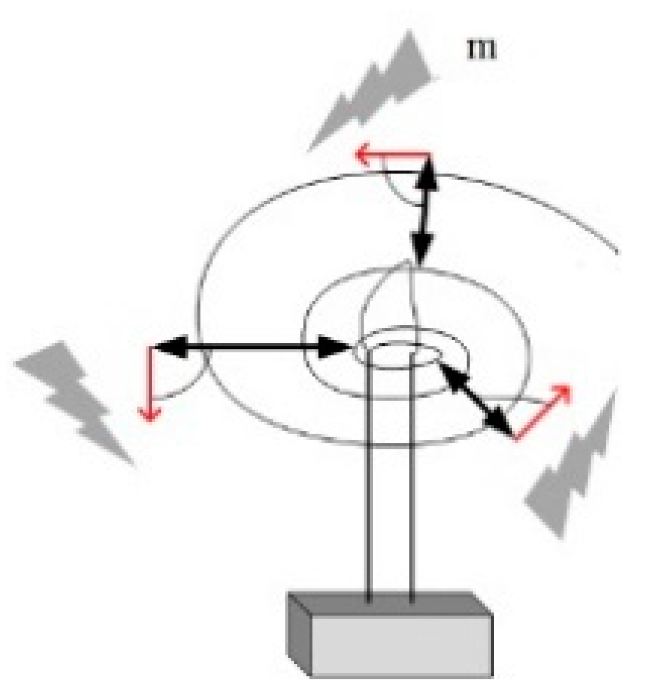
Moths use special navigational mechanisms for lateral orientation during night flight. In this mechanism, the moth flies by maintaining a fixed angle of its light relative to the moon. Since the moon is so far away from the moth, the moth uses this near-parallel light near the surface to stay in a straight line. Although lateral orientation is effective, moths are often observed to circle the source repeatedly until they are exhausted. In fact, moths are fooled by the fact that there are many artificial or natural point light sources. This is due to the low efficiency of lateral positioning; only under the condition of the light source being very far away is it helpful to the moths for maintaining straight flying movement, and there is a lot of artificial or natural light other than that resulting from moths being very close to the moon; when the moths continue to use as a light source the light emitted from a fixed angle, failure can lead to navigation and produce, as shown in Figure 1, a deadly spiral flight path.
2.2. Basic Model of Moth-Flame Optimization Algorithm
In the MFO algorithm, the moth is assumed to be the candidate solution to the problem, and the variable to be solved is the position of the moth in space. By changing their position vectors, moths can fly in one, two, three and even higher dimensions. Since the MFO algorithm is essentially a swarm intelligence optimization algorithm, the moth population can be represented as follows in the matrix:
where n represents the number of moths and d represents the number of control variables to be solved (dimension of the optimization problem). For these moths, it is also assumed that there is a corresponding list of fitness value vectors, represented as follows:
In the MFO algorithm, each moth is required to update its own position only with the unique flame corresponding to it, so as to avoid the algorithm falling into the local optimal value, which greatly enhances the algorithm’s global search ability. Therefore, the positions of the flame and moth in the search space are variable matrices of the same dimension.
For these flames, it is also assumed that there exists a corresponding column of fitness value vectors, represented as follows:
During the iteration process, the update strategy of the variables in the two matrices is different. Moths are actually search individuals that move within the search space, and the flame is the best position that the iteratively optimized moths can achieve so far. Each individual moth surrounds a corresponding flame, and when a better solution is found, it is updated to the location of the flame in the next generation. With this mechanism, the algorithm is able to find the global optimal solution.
In order to carry out mathematical modeling for the flight behavior of a moth to a flame, the updating mechanism for the position of each moth relative to a flame can be expressed by the following equation:
where represents the ith moth, represents the jth flame and represents the helical function.
This function satisfies the following conditions:
- (1)
- The initial point of the helical function is selected from the initial space position of the moth;
- (2)
- The end point of the spiral is the space position corresponding to the contemporary flame;
- (3)
- The fluctuation range of the spiral should not exceed its search space.
According to the above conditions, the helical function of moth flight path is defined as follows:
where is the linear distance between the ith moth and the jth flame, is the logarithmic helix shape constant defined, and the path coefficient is the random number in [−1,1]. The magnitude of t is represented by Formula (7), where a is represented by Formula (8), and its magnitude decreases linearly from −1 to −2. The expression of is as follows:
Formula (9) simulates the path of the moth’s spiral flight. From this equation, it can be seen that the next position of the moth’s renewal is determined by the flame it surrounds in the contemporary era. The coefficient () in the helix function represents the distance between the moth’s position and the flame in the next optimization iteration, () represents the closest position to the flame, and represents the farthest position. The spiral equation shows that moths can fly around the flame rather than just in the space between them, thus ensuring the algorithm’s global search capability and local development capability.
When this model is adopted, it has the following characteristics:
- (1)
- By randomly selecting parameters , a moth can converge to any field of flame;
- (2)
- The smaller the value of , the closer the moth is to the flame;
- (3)
- As the moth gets closer and closer to the flame, its position around the flame is updated more and more rapidly.
The above flame position update mechanism can ensure the local development ability of the moth around the flame. To improve the chances of finding a better solution, the best solution found in the current generation is used as the location of the next generation of moths around the flame. Therefore, the flame position matrix usually contains the optimal solution currently found. In the optimization process, each moth updates its position according to the matrix . The path coefficient in the MFO algorithm are internal random numbers in [, and the variable decreases linearly according to the number of iterations in the optimization iteration process in [. In this process, the moth will approach the flame in its corresponding sequence more precisely as the iteration progresses. After each iteration, the flames are reordered based on fitness values. In the next generation, the moth updates its position according to the flame corresponding to it in the updated sequence. The first moth always updates its position relative to the flame with the best fitness value, and the last moth updates its position relative to the one with the worst fitness value in the list.
If each location update of moths is based on different locations in the search space, the local development capability of the algorithm will be reduced. In order to solve this problem, an adaptive mechanism is proposed for the number of flames, so that the number of flames can be reduced adaptively in the iterative process, thus balancing the algorithm’s global search capability and local development capability in the search space. The formula is as follows:
where is the current iteration number, is the initial maximum number of flames set, and represents the maximum number of iterations set. At the same time, due to flame reduction, the moth corresponding to the reduced flame in the sequence in each generation updates its position according to the flame with the worst current fitness value.
3. An Improved Moth-Flame Optimization Algorithm (IMFO)
In order to improve the global exploration ability of the original moth-flame optimization algorithm, adding the Lévy flight mechanism to the global exploration flight path of the moth can effectively expand the search space of the moth and improve the global search ability of the moth. While improving the global search ability of the algorithm, the local development ability of the algorithm is also improved by means of the update strategy based on greedy reservation. By combining the two strategies, the global search and local development capabilities of the algorithm can be effectively balanced, and the original algorithm can be improved.
3.1. Lévy Flight
Lévy flight [27] is a Markov process proposed by Paul Pierre Lévy, a famous French mathematician. A random walk is a mathematical statistical model that consists of a series of trajectories, each of which is random, used to represent irregular patterns of change. Lévy flight is a typical random walk mechanism, which represents a class of non-Gaussian stochastic processes and is related to the Lévy stable distribution. Its steady increment obeys the Lévy steady distribution. Lévy flight is characterized by many small steps but occasionally large steps, so that moving entities do not repeatedly search the same place, changing the behavior of a system. Although its motion direction is random, its motion step size has an exponential rate distribution. The combination of the moth-flame optimization algorithm and Lévy flight strategy can expand the search range of the algorithm, increase the diversity of the population, and make it easier for the algorithm to jump out of the local optimum.
For example, bats with Lévy’s flight behavior [27] are more likely to find food. At present, Lévy flight has been successfully applied to the optimization field, and the results show that Lévy flight has achieved satisfactory results. In the global update of the moth algorithm, the Lévy flight mechanism is added to expand the search scope of the algorithm, making it difficult for the algorithm to fall into local optimization. The improved Formula (11) is:
Here, t is the current iteration number, Mi is the ith moth, Fj is the jth flame, and Di is the distance between the ith moth and the jth flame. When the moth spiral flight updates its position, the addition of the Lévy flight mechanism can expand the search range of the moth and prevent it from falling into local optimization. The formula of Lévy flight is as follows [28]:
where r1 and r2 are random numbers between [0,1], is a constant 1.5, and the formula is as follows:
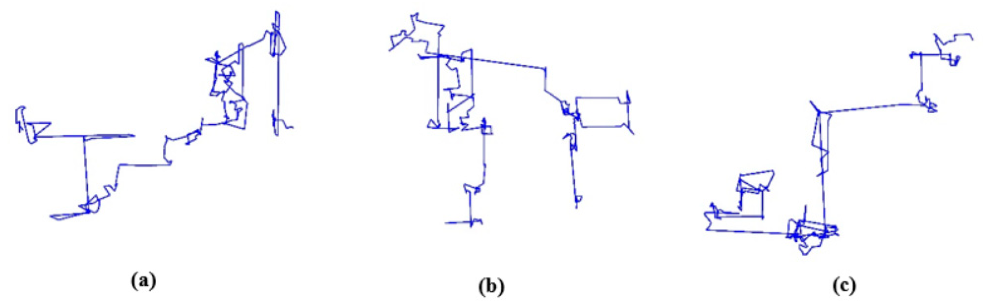
where ; 200 step sizes have been drawn to form a consecutive 50 steps of Lévy flight as shown in Figure 2.
This article describes three Lévy flight paths as shown in Figure 2a–c. In the picture, the parameters are set as follows: is a constant 1.5, the number of steps is set as 200, and the number of dimensions is set as 10. As we can see, the paths in the three pictures are very different, which can effectively demonstrate that Lévy flight is a random walk mechanism. However, there are some long walks after short walks. In Lévy flights, exploratory local searches over short distances are the same as occasional longer walks, ensuring that the system does not fall into local optimality. Lévy flight maximizes resource search efficiency in uncertain environments. The random number algorithm is used to draw three Lévy flight paths with 200 consecutive steps on the plane, as shown in Figure 2. The strategy ensures that the improved moth-flame optimization algorithm avoids falling into local optimality.
3.2. Dimension-By-Dimension Evaluation Strategy
In the standard MFO algorithm, the full-dimension update evaluation strategy is adopted; that is, after updating all the dimension information, the updated solution is evaluated according to the value of the objective function. This method, [29], will, to some extent, obscure the information of the evolutionary dimension, waste the known evaluation times and worsen the convergence rate of the solution. At the same time, such an updating mode causes mutual interference between dimensions, which affects the convergence speed and optimization accuracy of the algorithm. Assuming that the objective function and the global optimal solution for , the optimal value of . Supposing the algorithm iteration solution is the first k generation of the ith solution for , the objective function value of . In the process of the iteration algorithm, the first hypothesis according to Formula (5) is that the overall updates to (0, −1, 0), resulting in the objective function value of . According to the objective function evaluation mechanism, ; the updated solution compared to the original objective function value is big, so the algorithm will retain the original objective function values and discard the updated value of the target function. However, the value of the updated solution in the first dimension evolves from the previous 0.5 to 0 and and the value of the third dimension evolves from 0.5 to 0, but since the value of the second dimension degrades from 0 to −1, the algorithm will discard the updated solution directly in the evaluation strategy of the full dimension update. Therefore, this evaluation mechanism will waste the evaluation times of the solution and worsen the convergence rate.
The improved dimension-by-dimension update strategy can prevent the above problems. The improved moth-flame optimization algorithm based on the greedy retention of the one-dimension evaluation strategy can consider the information updating of each dimension. The idea of this strategy is as follows: the values of one dimension are updated to form a new solution with the values of other dimensions; then, the new solution is evaluated according to the fitness of the objective function. If the quality of the current solution can be improved, the updated result of this dimension for the solution is retained. Otherwise, the updated current dimension value is discarded, the previous dimension information is kept, and the next dimension is updated, using this greedy retention method until the update of each dimension is completed. For example, suppose that the value of the first dimension of the algorithm is updated to 0 in the iteration process, the solution after the dimension update is (0,0,0.5), and the value of the objective function obtained by the update is . At this point, the algorithm retains the update of the first dimension and then updates the next dimension. If the updated value of the first dimension is 1, the updated solution is (0,0,0.5), and the value of the objective function is , the algorithm based on the dimension-by-dimension evaluation update mechanism will discard the update of the current dimension and carry out the update operation of the next dimension. This updating mechanism can prevent the waste of the number of evaluation solutions and optimize the convergence speed of the algorithm.
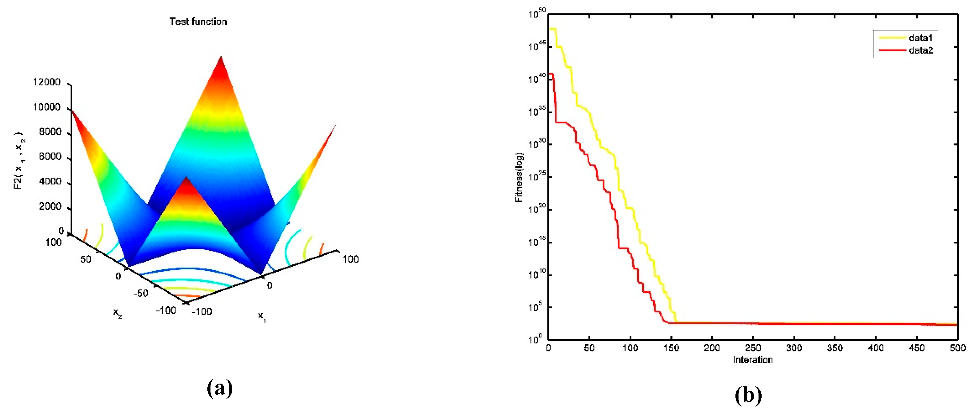
In order to demonstrate the effectiveness of dimension-by-dimension valuation, the F2 test function shown in Figure 3a is randomly selected in this paper. The formula for this function is The function definition field is [−10,10], and the theoretical optimal value is 0. This function is a continuous unimodal function., which is mostly used to investigate the optimization accuracy of the algorithm. When the dimension of function F2 (a) is set to 100, date1 (b) represents the convergence trend of the standard moth-flame optimization algorithm for function F2, and date2 (b) represents the convergence trend of the algorithm for function F2 after adding dimension-by-dimension evaluation into the standard algorithm in Figure 3b. It can be seen that the algorithm of dimension-by-dimension evaluation can make the convergence of the function faster.
The evolutionary dimension of the solution is paid attention to by using the strategy of updating dimension-by-dimension based on greedy reservation. Eliminating the influence of the degenerate dimension on the solution saves the evaluation time wasted by random updating. It can effectively suppress the interference between different dimensions, improve the convergence rate of the algorithm and improve the local development ability of the algorithm.
The pseudo-code of the improved algorithm is as follows:
| Algorithm 1 IMFO Algorithm Pseudo-Code |
| 1: Set population size N, maximum number of iterations , and dimension of objective function Dim |
| 2: Initializes the moth position |
| 3: while (t < ) do |
| 4: Update the flame position according to Equation (9) |
| 5: Transboundary treatment of moths |
| 6: if |
| 7: find the moth and update the position of the flame according to the moth |
| 8: else |
| 9: find the moth and update the position of the flame according to the moth |
| 10: end |
| 11: Update according to Equation (8) |
| 12: for |
| 13: for |
| 14: if |
| 15: Update Di according to Equation (9) |
| 16: Update S (Mi, Fj) according to Equation (11) |
| 17: end |
| 18: if |
| 19: Update Di according to Equation (9) |
| 20: Update S (Mi, Fj) according to Equation (6) |
| 21: end |
| 22: end |
| 23: end |
| 24: Update moth position and fitness value through dimension-by-dimension evaluation |
| 25: t = t +1 |
| 26: end while |
| 27: Output the best search location and its fitness value |
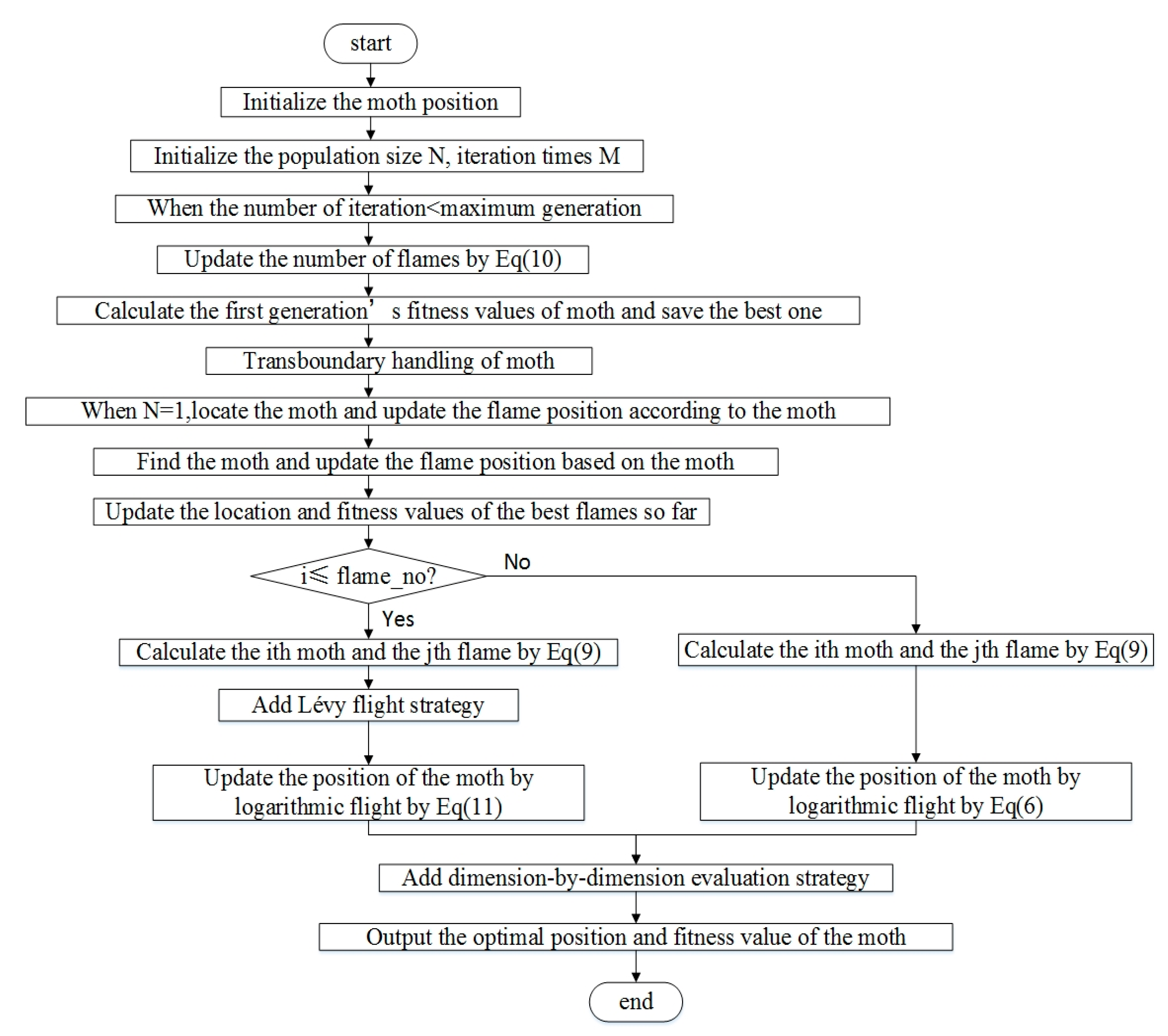
The flowchart in Figure 4 of the improved algorithm is as follows. It can be seen that the improvements are as follows: first, the Lévy flight mechanism is added to the global search, which can expand the global search capability of the algorithm and prevent the algorithm falling into local optimization. Secondly, adding the dimensionality evaluation mechanism into the algorithm can effectively balance the global exploration ability and local development ability, reduce the running times of the algorithm and improve the running efficiency of the algorithm. When calculating 23 test functions, the precision of the algorithm can be improved and the function can be converged faster. In solving engineering problems, better solutions can be obtained than with other algorithms.
Through the flowchart, we can clearly see the improved moth flame algorithm process and improvements compared with the original moth flame algorithm. The Lévy flight and dimension-by-dimension evaluation mechanism can balance the global search capability and local developability of the algorithm so that the algorithm can achieve better results in solving engineering problems.
4. Experimental Studies and Comparisons
In this section, we describe the basic expression, upper and lower bounds, and theoretical optimal value of the test function. Then, we selected nine comparison algorithms and set their parameters. Then, the performance of nine comparison algorithms in 13 non-fixed dimensions and 10 fixed dimensions was compared through experimental data. Thirteen functions of non-fixed dimensions were set up in the dimensions 10,30 and 100, respectively. The convergence precision of the algorithm is compared in different aspects. Finally, the convergence of the algorithm is tested and compared.
4.1. Test Function and Experimental Parameter Setting
In the experiment, 23 benchmark functions were selected according to [30] and [31], among which the first 13 functions were functions of variable dimensions and the last 10 functions were functions of fixed dimensions. A complete set of benchmark functions, consisting of 23 different functions (single mode and multi-mode), is used to evaluate the performance of the algorithm. The definition, function image, upper and lower bounds, dimension settings and minimum of the reference function are shown in Table 1 and Table 2. We introduce reference functions such as F1, F2 and F3, up to F23. For F1 to F7, there is a single peak optimization problem with an extreme point in a given search area. These functions are used to study the convergence rate and optimization accuracy of the algorithm. F8–F23 are multi-modal optimization functions with multiple local extremum points in a given search area. They are used to evaluate the ability to jump out of local optima and seek global optima. In addition, the dimensions of d = 10, d = 30 and d = 100 are set for the first 13 functions in this paper, so as to test different algorithms.
Meanwhile, eight comparison algorithms were selected, namely, the original moth-flame algorithm (MFO), sine and cosine algorithm (SCA), bat algorithm (BA), spotted hyena algorithm (SHO), particle swarm optimization algorithm (PSO), whale algorithm (WOA), grey wolf algorithm (GWO) and salp swarm algorithm (SSA). The parameter settings in these comparison algorithms are shown in Table 3. In addition to the parameter settings in Table 3, the population number of each algorithm is set to 30, and the number of iterations is set to 1000. The experiment was conducted on the 64-bit operating system of Windows 7 with the software MATLAB 2014a version, and the processor was an Intel(R) Core (TM) i5-5200U [email protected] GHz 2.20 GHz with 4.00 GB of RAM.
Table 1 shows the expressions, images and upper and lower bounds of 13 benchmark functions. There, L represents the lower bound, U represents the upper bound of the functions, D represents the dimension of the function and fmin represents the theoretical optimal value.
Table 2 shows the ten complex dimension test functions.
4.2. Comparison of Algorithm Parameter Settings
Table 3 shows the parameter settings of the different algorithms during the experiment. In addition, in the process of running the algorithm, the population quantities were set to 30 and the maximum number of iterations was set to 1000.
4.3. Comparison with Other Algorithms
In order to verify the effectiveness of the IMFO algorithm, eight different algorithms are used to test the mathematical benchmark functions in this section. Different algorithm processing function run results are shown in Table 4, where N/A means that the algorithm is not suitable for solving this function. Table 4 shows the comparison of the means and standard deviations of the nine algorithms when the dimension is 10. It should be noted that the best optimal solution obtained is highlighted in bold font.
As shown in the Table 4 results, we found that the improved moth-flame optimization algorithm is better than the other algorithms for solving the average (Ave) and standard deviation (Std) values of the benchmark functions F1, F3, F4, F7, F9, F10, F11, F15, F16, F17, F18 and F19. In addition, the standard deviations (Std) of the base functions F5, F21, F22 and F23 of the improved IMFO algorithm can obtain the optimal value. The best average can also be obtained for F8. Particle swarm optimization (PSO) ranks second for the performance of F6, F12 and F13. Additionally, the spotted hyena optimizer (SHO) obtains the best value on the function F2, and it obtains the minimum average on the function F16. The salp swarm algorithm (SSA) obtains the best value on the function F14. Finally, as we can see, BA can obtain the minimum average on the function F5. In addition, GWO can obtain the minimum average on the functions F17, F21, F22 and F23. SCA has the best stability in solving the function F8.
The results indicate the superiority of the proposed algorithm. Analysis of the averages and standard deviations reveals that the proposed IMFO algorithm shows competitive performance in comparison with the compared algorithms. The comparison results for the selected unimodal functions (F1–F7) are shown in Table 4. Note that, except for F2, F5 and F6, IMFO is better than the compared eight algorithms for all the other test functions. In particular, a huge improvement is achieved for the benchmark functions F1 and F3. These results verify that IMFO has excellent optimization accuracy with one-global minimal functions. For the multi-modal functions (F8–F23), IMFO also performs better than other algorithms. IMFO can find superior average results for the test functions F8, F9, F10, F11, F15, F16, F17, F18, F19 and F20. These results mean that the improved IMFO algorithm has a good ability to jump out of local optima and seek global optima.
It is obvious that IMFO better solves these 23 benchmark functions than the other algorithms. At the same time, it can be seen from Table 4 that the variance of the IMFO algorithm on 16 test functions is the minimum value of the nine comparison functions, indicating that the improved moth-flame optimization algorithm has good robustness.
Table 5 shows a comparison of the improved algorithm with the other algorithms for the first 13 functions, when d = 30, in terms of experimental data.
It can be seen that, compared with the other algorithms, IMFO algorithm for functions F3, F4, F9, F10, F11 and F12 obtains minimum values. Secondly, the WOA algorithm is the best in solving function F1. SCA performs the most stably in solving the function F8. When d = 30, SHO can still obtain the minimum value in solving function F2. At this point, the GWO algorithm performs best in solving the function F7. The PSO algorithm can obtain the minimum value when solving F13 and the minimum average value when solving F6. Finally, the BA algorithm can obtain the minimum average value when solving F5, and it has the best robustness and the most stable result when solving F6. Therefore, when d = 30, it can be seen from the solution results of the nine algorithms on the 13 test functions that the solution effect of IMFO is still optimal compared with that of the other algorithms.
Table 6 compares the improved algorithm with the other algorithms for the first 13 functions in terms of experimental data, when d = 100.
Compared with other algorithms, the IMFO algorithm for the functions F3, F4, F7, F9, F10 and F11 obtains minimum values with a significant effect. At the same time, when solving functions F6, F8 and F13, the minimum variance can be obtained, which indicates that the IMFO algorithm has good stability and strong robustness in solving high-dimensional problems. At this point, compared with d = 10 and d = 30, the WOA algorithm shows obvious advantages in solving the results of functions. It has the best performance in solving functions F1, F2 and F5. Meanwhile, it can obtain the minimum average when solving functions F8, F12 and F13. The BA algorithm can obtain the minimum average value when solving F6 and the best stability when solving F12. However, when the dimension increases, MFO, SCA, BA, SHO, PSO, GWO and SSA produce poor results. The improved moth-flame optimization algorithm and the whale algorithm produce better results, but the improved moth-flame optimization algorithm is still the best on the whole.
4.4. Convergence Test
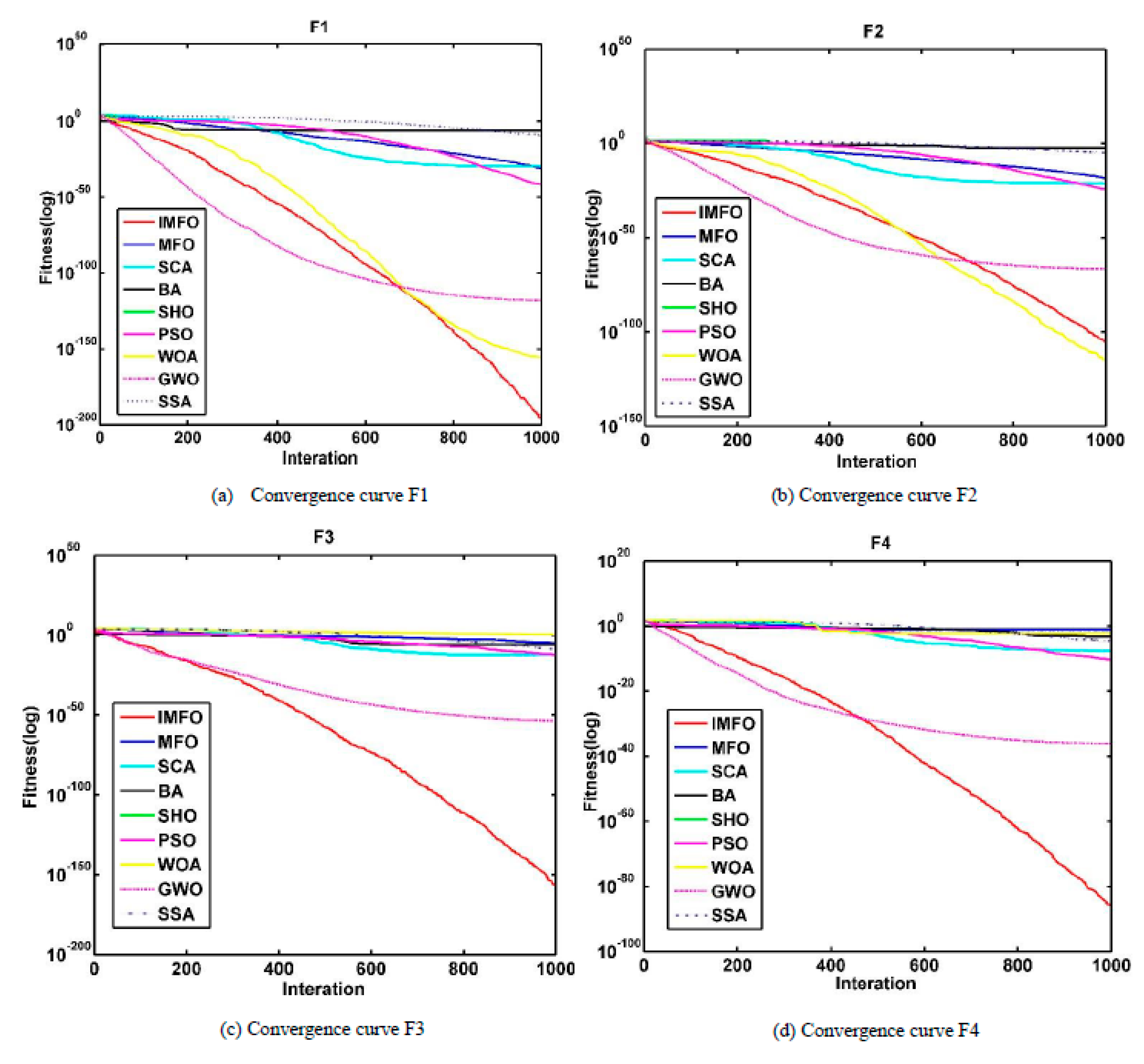
A convergence test refers to drawing different convergence images when running different test functions with different algorithms, through which the convergence speed and convergence accuracy of the algorithm can be compared. In order to further study the performance and effect of the improved algorithm, this section tests the convergence of nine different algorithms under the conditions that the dimension d of the 13 functions from F1 to F13 is 10, the maximum number of iterations is 1000 and the population number is 30, and analyzes the convergence speed and calculation accuracy of the algorithm.
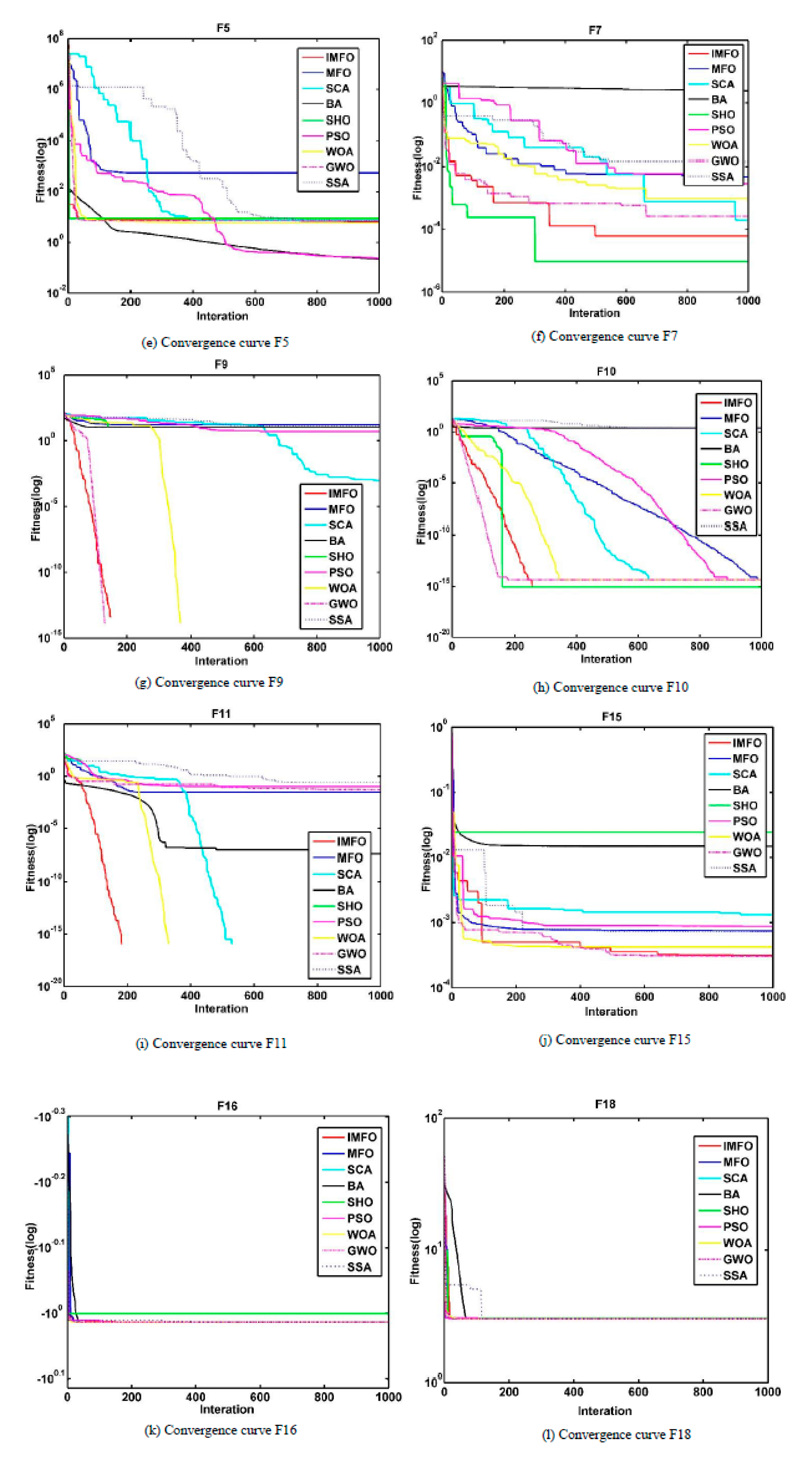
To further illustrate the advantages of the improved algorithm, the convergence behavior is shown in Figure 5. According to the convergence curve shown in Figure 5, it can be verified that the proposed IMFO converges faster than the other algorithms. The results show that the improved algorithm based on Lévy flight and dimension-by-dimension evaluation can effectively improve the convergence trend of the original algorithm. Twelve functions are selected to demonstrate the convergence test of the algorithm. It can be seen from the image in (a) to (l) that the improved moth-flame optimization algorithm for those functions has a better convergence than the original moth-flame optimization algorithm.
Compared with the other algorithms, the improved moth-flame optimization algorithm has faster convergence speed and higher calculation accuracy on the 10 functions F1 (a), F2 (b), F3 (c), F4 (d), F5 (e), F7 (f), F9 (g), F10 (h), F11 (i) and F15 (j). On the two function F16 (k) and F18 (l), there is not much difference in the convergence trends for those algorithms. As we can see, the improved moth-flame optimization algorithm converges the most quickly and has higher convergence precision on the functions F1 (a), F3 (c), F4 (d) and F11 (i). On the function F2 (b), GWO, IMFO and WOA perform better than the other algorithms. GWO has best convergence speed at the beginning, but its later convergence is slow. IMFO and WOA converge faster than GWO, and they have smaller convergence. However, WOA is slightly better than IMFO in the solution of the function F2 (b). On the functions F1 (a) and F4 (d), although the GWO algorithm converges quickly in the early stage, the IMFO algorithm converges the fastest in the later period. Furthermore, the value of function F2 (b) solved by the IMFO algorithm is the smallest compared with that with the other algorithms. On the functions F3 (c) and F11 (i), the IMFO algorithm has an absolute advantage over the other algorithms. On the function F7 (f), the solution with SCA is slightly better than that with IMFO. The GWO algorithm almost has the same result as the IMFO algorithm when solving the function F9. The IMFO algorithm ranks third in the result for solving the function F5 (e). The SHO algorithm has the best performance in solving the function F10 (h), which has better convergence speed than the IMFO algorithm. However, they have the same convergence value. On the function F15 (j), the WOA, GWO and IMFO algorithms have almost similar performance in solving it. Generally, the IMFO algorithm has faster convergence speed and higher convergence precision than the other algorithms.
4.5. Statistical Analysis
Derrac et al. proposed in literature [32] that statistical tests should be carried out to evaluate the performance of improved evolutionary algorithms. In other words, comparing algorithms based on average, standard deviation and convergence analysis is not enough. Statistical tests are needed to verify that the proposed improved algorithm shows significant improvement and advantages over other existing algorithms. In this section, the Wilcoxon rank sum test and Friedman test are used to verify that the proposed IMFO algorithm has significant improvements and advantages over other comparison algorithms.
In order to determine whether each result of IMFO is statistically significantly different from the best results of the other algorithms, the Wilcoxon rank sum test was used at the significance level of 5%. The dimension d of the 13 functions from F1 to F13 is 10, the maximum number of iterations is 1000, and the population number is 30. The p-value for Wilcoxon’s rank-sum test on the benchmark functions was calculated based on the results of 30 independent running algorithms.
In Table 7, the p values calculated in the Wilcoxon rank sum tests for all the benchmark functions and other algorithms are given. For example, if the best algorithm is IMFO, paired comparisons are made between IMFO and MFO, IMFO and SCA, and so on. Because the best algorithm cannot be compared to itself, the best algorithm in each function is marked N/A, meaning “not applicable”. This means that the corresponding algorithm can compare itself with no statistical data in the rank sum test. In addition, in Table 7, N/A means not applicable. According to Derrac et al., p < 0.05 can be considered as a strong indicator for rejecting the null hypothesis. According to the results in Table 7, the p value of IMFO is basically less than 0.05. The p value was greater than 0.05 only for F5, F8, F14 and F19 for IMFO vs. MFO, F14 for IMFO vs. SCA, F18 for IMFO vs. BA, F14 and F20 for IMFO vs. PSO, F8 and F9 for IMFO vs. WOA, and F5 and F15 for IMFO vs. GWO. This shows that the superiority of the algorithm is statistically significant. In other words, the IMFO algorithm has higher convergence precision than the other algorithms.
Furthermore, to make the statistical test results more convincing, we performed the Friedman test on the average values calculated by the nine algorithms on 23 benchmark functions in Section 4.3. The significance level was set as 0.05. When the p value was less than 0.05, it could be considered that several algorithms had statistically significant differences. When the algorithm’s p value is greater than the significance level of 0.05, it can be considered that there is no statistically significant difference between the algorithms.
According to the calculation results in Table 8, when the dimension of the current 13 functions is set to 10, the rank means of the nine algorithms are 2.71 (IMFO), 5.45 (MFO), 5.52 (SCA), 6.52 (BA), 7.86 (SHO), 3.38 (PSO), 4.24 (WOA), 4.19 (GWO) and 5.12 (SSA). The priority order is IMFO, PSO, GWO, WOA, SSA, MFO, SCA, BA and SHO. Here, ; this indicates that there are significant differences among the nine algorithms.
Similarly, when the dimension of the first 13 functions is set to 30, the rank means of the nine algorithms are 2.92 (IMFO), 8.25 (MFO), 6.83 (SCA), 4.92 (BA), 5.67 (SHO), 4.17 (PSO), 3.50 (WOA), 3.17 (GWO) and 5.58(SSA). The priority order is IMFO, GWO, WOA, PSO, BA, SSA, SHO, SCA and MFO. Here, ; this indicates that there are significant differences among the nine algorithms.
Finally, when the dimension of the first 13 functions is set to 100, the rank means of the nine algorithms are 2.63 (IMFO), 7.17 (MFO), 6.83 (SCA), 4.00 (BA), 5.83 (SHO), 2.79 (PSO), 3.08 (WOA), 6.25 (GWO) and 6.42 (SSA). The priority order is IMFO, PSO, WOA, BA, SHO, GWO, SSA, SCA and MFO. Here, ; this indicates that there are significant differences among the nine algorithms.
In the fourth chapter, eight comparison algorithms are selected to conduct 30 experiments and the mean values and variance of 23 test functions are solved, which are compared with those from the improved moth-flame optimization algorithm. According to the experimental data, the IMFO algorithm has good stability in solving function values. In addition, 12 of the 23 test functions were randomly selected for convergence analysis in this paper. As can be seen from the convergence trend graph of Figure 5, the IMFO algorithm has better convergence speed and relatively high convergence accuracy on the whole. Finally, both the Wilcoxon rank sum test and Friedman test indicate that the improved IMFO algorithm has good performance. In Chapter 5, the improved moth-flame optimization algorithm is applied to solve four engineering problems—namely, pressure vessel, compression/tension spring, welded beam and trusses design problems—to illustrate the application of the IMFO algorithm in practice.
5. IMFO for Engineering Problems
This subsection analyzes the performance and efficiency of IMFO by solving four constrained real engineering problems, namely, the pressure vessel problem, tension/compression spring problem, welding beam problem and three-bar truss problem. These problems have many inequality constraints, so the IMFO tries to handle them in processing. The number of solutions in all the experiments is 30, and the maximum number of iterations is 1000.
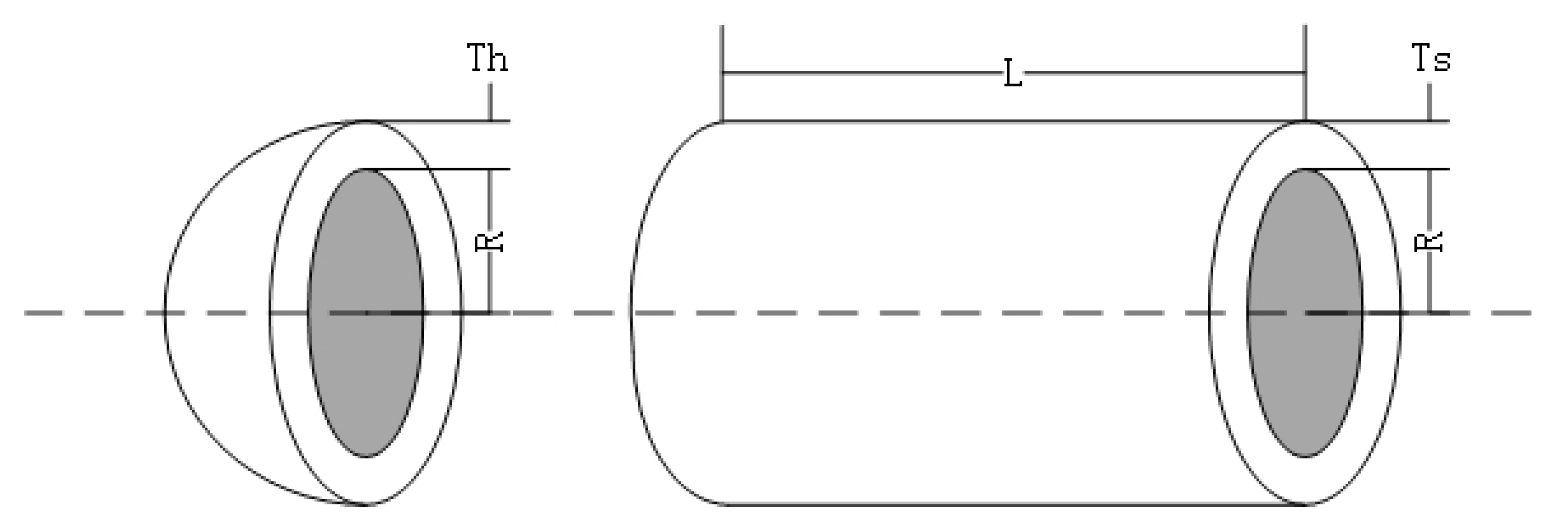
5.1. Pressure Vessel Design Problem
The purpose of the pressure vessel problem is to minimize the total cost of the cylindrical pressure vessel [33]. There are four design variables and four constraints based on the thickness of the shell (), the thickness of the head (), the internal radius (R), and the length of the cylindrical section without considering the head (L). Figure 6 shows the pressure vessel and parameters involved in the design. The design can be expressed as follows:
Consider
Objective function:
Subject to
Variable ranges:
In this section, the pressure vessel problem is solved by the IMFO algorithm, and the results are compared to those from the MFO [1], OMFO [22], ES [31], CSDE [33], CPSO [34], LFD [35], WOA [36], MOSCA [37], RDWOA [38], CCMWOA [39], LWOA [40], GA [41], BFGSOLMFO [42] and IMFO [43]. Table 9 shows the IMFO is able to obtain the best solution for this problem. The results show that the IMFO algorithm can outperform all the other algorithms and outperform by MOSCA [37] and IMFO [43].
As can be seen from Table 9, when the four parameters , , R and L are set as 0.7781948, 0.3846621, 40.32097 and 199.9812, respectively, the minimum value of IMFO is 5885.3778. Compared with the other methods, IMFO achieves better results in the pressure vessel design problem. Therefore, this shows that the algorithm is feasible and effective in solving engineering problems with constraints.
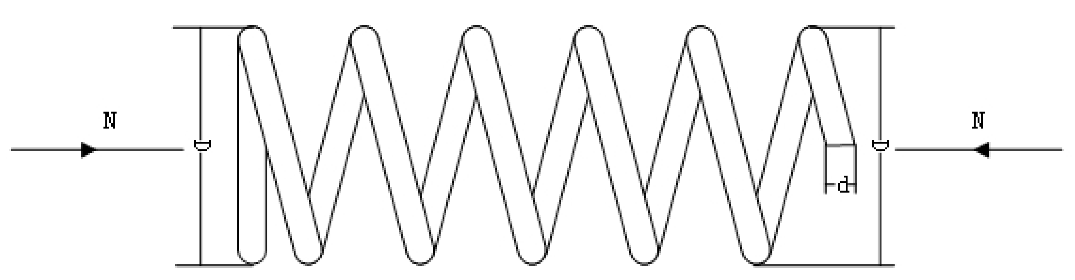
5.2. Compression/Tension Spring Design Problem
The goal of this design problem is to minimize the weight of the compression/tension spring [27]. Figure 7 shows the spring and parameters. In this problem, there are three variables and four constraints. These variables include the coil diameter (d), mean coil diameter (D) and number of effective coils (N). The mathematical model for this problem is:
Consider
Objective function:
Subject to
Variable ranges:
In this section, the compression/tension design problem is solved using the IMFO algorithm, and the results are compared to those from the MFO [1], LAFBA [27], ES [31], CPSO [34], LFD [35], WOA [36], CCMWOA [39], LWOA [40], GA [41] and RO [44]. Table 10 shows the decision variables and constraint values of the best solutions obtained by different methods. The results show that the IMFO algorithm can outperform all the other algorithms.
5.3. Welded Beam Design Problem
The objective of this model is to determine the minimum manufacturing cost [36]. Figure 8 shows the welded beam and parameters involved in the design. In this case, four variables affect the manufacturing cost, including the height of the reinforcement (t), the thickness of the weld (h), the thickness of the reinforcement (b) and the length of the reinforcement (l). The optimal design of this problem must satisfy the constraint conditions: shear stress (), bending stress in the beam (), deflection of the beam (), and buckling load (). The mathematical model of the problem can be described as:
Consider
Objective function:
Subject to
Variable ranges:
The Where
Table 11 presents the best weights and the optimal values for the decision variables from IMFO and several other algorithms LMFO [26], LAFBA [27], CSDE [33], CPSO [34], LFD [35], WOA [36], RO [44] and SFO [45]. The statistical results show the IMFO algorithm can outperform six algorithms and outperform by LMFO [26] and CSDE [33].
5.4. Three-Bar Truss Design Problem
The design of a three-bar truss is a structural optimization problem in the field of civil engineering [41]. Figure 9 shows the three-bar truss and parameters involved in the design. In order to minimize the volume of the three-bar truss, the constraints are stressed on each truss member. The three-bar truss design problem has a difficult constrained search space, so it is applied to evaluate the optimization power of the proposed algorithms. The formulation of this problem is as follows:
Consider
Objective function:
Subject to
Variable range
This problem has been solved by many researchers as a benchmark optimization problem in the literature. The three-bar truss design problem is solved using the IMFO algorithm, and the results are compared to those from SFO [45], m-SCA [46], WOA [36], Tsai [47] and MFO [1]. The results show that IMFO can outperform all the other algorithms except Tsai, which outperforms it [47].
Table 12 shows that IMFO is more competitive than the other four algorithms except Tsai [47] in terms of accuracy and function evolution cost. The best objective function value for the three-bar truss design problem solved with the IMFO algorithm is 263.8959, and the two parameters are 0.78899 and 0.40736.
In this chapter, we can see that the improved moth-flame optimization algorithm is very effective in solving the above four engineering problems. Especially in the solution of the pressure vessel problem, the effect is very obvious. Therefore, it can be seen from this section that the improved algorithm has good optimization performance for solving the problem.
6. Conclusions and Future Work
In this article, two strategies are used: Lévy flight and dimension-by-dimension evaluation. Lévy flight is used in the global search of moths. In order to further improve the global search performance of moths, Lévy flight is added into the update mechanism of the moths to expand the global search capability of the algorithm. The Lévy flight mechanism plays the role of random walk, and its application in the process of the global search of moths can help moths to better update their position, effectively expand the search range of the moths, and improve the global search ability of the algorithm. In the overall operation mechanism of the algorithm, adding the dimension-by-dimension evaluation mechanism can effectively improve the operation efficiency of the algorithm and balance the global search and local development. Dimension-by-dimension evaluation can effectively evaluate the solution of each dimension obtained by the algorithm. If the current solution is better than the initial solution, the current solution is retained and the next dimension is updated. On the contrary, if the current solution obtained after updating a dimension is worse than the original solution, the update of the current solution is abandoned and the update operation of the next dimension is continued. By adding a dimension-by-dimension evaluation mechanism to the algorithm, the evaluation times of the solution can be effectively used to avoid unnecessary waste, so as to improve the convergence speed of the algorithm. The improved algorithm can obtain good results when solving 23 benchmark functions. On the whole, it has a fast convergence speed and high convergence precision. The results of the experiments show that the proposed algorithm applying the Wilcoxon rank sum test and Friedman test on 23 benchmark functions has a better performance than the other compared algorithms. IMFO outperforms the compared algorithms in terms of the statistical results and convergence rate. At the same time, the improved algorithm can obtain better results in solving four engineering problems, especially in the design of pressure vessels.
There are several suggestions as future directions for the improved moth-flame algorithm: (1) enhancing the theoretical research of the IMFO algorithm; (2) improving the mobility mechanism [48] based on the position of the current optimal moth to enable the moth to move with global orientation and expand the sharing of information between moths to improve the overall evolutionary optimization performance of the IMFO algorithm; (3) combining the improved moth-flame optimization algorithm with other algorithms such as the differential evolution (DE) algorithm [49] to further improve the performance of the IMFO algorithm; (4) investigating how to extend the IMFO algorithm to handle other constrained optimizations, multi-objective optimizations, and combinatorial optimization problems. The application of IMFO is desirable for solving more complex real-world problems.
Author Contributions
Conceptualization, supervision, writing—review and editing, funding acquisition, Y.L.; investigation, data curation, writing—original draft preparation, X.Z.; methodology, software, project administration, funding acquisition, J.L. All authors have read and agreed to the published version of the manuscript.
Funding
This work was supported by the National Natural Science Foundation of China (No. 71601071); the Science & Technology Department of Henan Province, China (No. 182102310886 and 162102110109); and a Ministry of Education Youth Foundation Project of Humanities and Social Sciences (No. 15YJC630079).
Acknowledgments
This work was supported by the National Natural Science Foundation of China (No. 71601071); the Science & Technology Department of Henan Province, China (No. 182102310886 and 162102110109); and a Ministry of Education Youth Foundation Project of Humanities and Social Sciences (No. 15YJC630079). We are particularly grateful to the suggestions of the editor and the anonymous reviewers which have greatly improved the quality of the paper.
Conflicts of Interest
The authors declare no conflict of interest.
References
- Mirjalili, S. Moth-flame optimization algorithm: A novel nature-inspired heuristic paradigm. Knowl.-Based. Syst. 2015, 89, 228–249. [Google Scholar] [CrossRef]
- Buch, H.; Trivedi, I.N. An Efficient Adaptive Moth Flame Optimization Algorithm for Solving large-scale Optimal Power Flow Problem with POZ, Iranian Journal of Science and Technology. Trans. Electr. Eng. 2019, 43, 1031–1051. [Google Scholar]
- Das, A.; Mandal, D.; Ghoshal, S.P.; Kar, R. Concentric circular antenna array synthesis for side lobe suppression using moth flame optimization. aeu-Int. J. Electron. Commun. 2018, 86, 177–184. [Google Scholar] [CrossRef]
- Ishiguro, S.; Endo, T.; Akio, Y. Loading pattern optimization for a PWR using multi-swarm Flame optimization Method with Predator. J. Nucl. Sci. Technol. 2019, 57, 523–536. [Google Scholar] [CrossRef]
- Rezk, H.; Ali, Z.M.; Abdalla, O.; Younis, O.; Gomaa, M.R.; Hashim, M. Hybrid moth-flame Optimization Algorithm and Incremental Conductance for Tracking Maximum Power of Solar PV/Thermoelectric System under Different Conditions. Mathematics 2019, 7, 875. [Google Scholar] [CrossRef] [Green Version]
- Taher, M.A.; Kamel, S.; Jurado, F.; Ebeed, M. An optimization algorithm for solving optimal power flow problem. Int. Trans. Electr. Energy. Syst. 2019, 29. [Google Scholar] [CrossRef]
- Tolba, M.A.; Zaki Diab, A.A.; Tulsky, V.N.; Abdelaziz, A.Y. LVCI approach for optimal allocation of distributed generations and allocation Banks in distribution based on moth-flame optimization algorithm. Electr. Eng. 2018, 100, 2059–2084. [Google Scholar] [CrossRef]
- Lei, X.; Fang, M.; Fujita, H. Moth-flame optimization-based algorithm with synthetic dynamic PPI networks for discovering protein complexes. Knowl-based Syst. 2019, 172, 76–85. [Google Scholar] [CrossRef]
- Sayed, G.I.; Hassanien, A.E. Moth-flame swarm optimization with neutrosophic sets for automatic mitosis detection in breast cancer histology images. Appl. Intell. 2017, 47, 397–408. [Google Scholar] [CrossRef]
- Mingjing, W.; Huiling, C.; Bo, Y.; Xuehua, Z.; Lufeng, H.; Zhennao, C.; Hui, H.; Changfei, T. Toward an optimal kernel extreme learning machine using a chaotic moth-flame optimization strategy with applications in medical diagnoses. Neurocomputing 2017, 267, 69–84. [Google Scholar]
- Elsakaan, A.A.; El-Sehiemy, R.A.; Kaddah, S.S.; Elsaid, M.L. An enhanced moth-flame optimizer for solving non-smooth economic dispatch problems with emissions. Energy 2018, 157, 1063–1078. [Google Scholar] [CrossRef]
- Jain, P.; Saxena, A. An opposition theory enabled moth flame optimizer for strategic bidding in uniform spot energy market. Eng. Sci. Technol. Int. J. 2019, 22, 1047–1067. [Google Scholar] [CrossRef]
- Khalilpourazari, S.; Pasandideh, S.H.R. Multi-item EOQ model with nonlinear unit holding cost and partial backordering: Moth-flame optimization algorithm. J. Ind. Prod. Eng. 2016, 34, 42–51. [Google Scholar] [CrossRef]
- Abdullah, A.; Faisae Ab Rashid, M.F.; Ponnambalam, S.G.; Ghazalli, Z. Energy efficient modeling and optimization for assembly sequence planning using moth flame optimization. Assem. Autom. 2019, 39, 356–368. [Google Scholar] [CrossRef]
- Ishtiaq, A.; Ahmed, S.; Khan, M.F.; Aadil, F.; Maqsood, M.; Khan, S. Intelligent clustering using moth flame optimizer for vehicular AD hoc networks. Int. J. Distrib. Sens. Netw. 2019, 15. [Google Scholar] [CrossRef]
- Wei Kun, L.; Wan Liang, W.; Li, L. Optimization of Water Resources Utilization by multi-objective moth-flame Algorithm. Water Resour. Manag. 2018, 32, 3303–3316. [Google Scholar]
- Ibrahim, R.A.; Elaziz, M.A.; Ewees, A.A.; Selim, I.M.; Songfeng, L. Galaxy images classification using hybrid brain storm optimization with moth flame optimization. J. Astron. Telesc. Instrum. Syst. 2018, 4, 038001. [Google Scholar] [CrossRef]
- Sharma, R.; Saha, A. Optimal test sequence generation in state based testing using moth flame optimization algorithm. J. Intell. & Fuzzy Syst. 2018, 35, 5203–5215. [Google Scholar]
- Singh, R.K.; Gangwar, S.; Singh, D.K.; Pathak, V.K. A novel hybridization of artificial neural network and moth-flame optimization (ann-mfo) for multi-objective optimization in magnetic finishing of aluminium 6060. Braz. Soc. Mech. Sci. Eng. 2019, 41, 1–19. [Google Scholar] [CrossRef]
- Elaziz, M.A.; Ewees, A.A.; Ibrahim, R.A.; Songfeng, L. Opposition-based moth-flame optimization by differential evolution for feature selection. Math. Comput. Simul. 2020, 168, 48–75. [Google Scholar] [CrossRef]
- Srikanth Reddy, K.; Panwar, L.K.; Panigrahi, B.K.; Kumar, R. Solution to unit commitment in power system operation planning using binary coded modified moth flame algorithm (BMMFOA): A flame selection based computational technique. J. Comput. Sci. 2018, 25, 298–317. [Google Scholar]
- Sapre, S.; Mini, S. Opposition-based moth flame optimization with Cauchy mutation and evolutionary boundary constraint handling for global optimization. Soft Comput. 2018, 23, 6023–6041. [Google Scholar] [CrossRef]
- Liwu, X.; Yuanzheng, L.; Kaicheng, L.; Gooi, H.B.; Zhiqiang, J.; Chao, W.; Nian, L. Enhanced Moth-flame Optimization Based on Cultural Learning and Gaussian Mutation. J. Bionic. Eng. 2018, 15, 751–763. [Google Scholar]
- Yueting, X.; Huiling, C.; Ali Asghar, H.; Jie, L.; Qian, Z.; Xuehua, Z.; Li, C. An efficient chaotic mutative mode-flame-inspired optimizer for global optimization tasks. Expert. Syst. Appl. 2019, 129, 135–155. [Google Scholar]
- Yueting, X.; Huilin g, C.; Jie, L.; Qian, Z.; Shan, J.; Xiaoqin, Z. Enhanced Moth-flame optimizer with mutation strategy for global optimization. Inf. Sci. 2019, 492, 181–203. [Google Scholar]
- Zhiming, L.; Yongquan, Z.; Sen, Z.; Junmin, S. Lévy-Flight Moth-Flame Algorithm for Function Optimization and Engineering Design Problems. Math. Probl. Eng. 2016, 2016, 22. [Google Scholar]
- Li, Y.; Li, X.T.; Liu, J.S.; Ximing, R. An Improved Bat Algorithm Based on Lévy Flights and Adjustment Factors. Symmetry 2019, 11, 925. [Google Scholar] [CrossRef] [Green Version]
- Yang, X.S.; Karamanoglu, M.; He, X. Flower pollination algorithm: A novel approach for multiobjective optimization. Eng. Optim. 2014, 46, 1222–1237. [Google Scholar] [CrossRef] [Green Version]
- Lijin, W.; Yilong, Y.; Wan, Z. Search algorithm of cuckoo. J. Softw. 2013, 24, 2687–2698. [Google Scholar]
- Chao, L.; Liang, G.; Jin, Y. Grey wolf optimizer with cellular topological structure. Expert Syst. Appl. 2018, 107, 89–114. [Google Scholar]
- Pei, H.; Jeng-Shyang, P.; Shu-Chuan, C. Improved Binary Grey Wolf Optimizer and Its application for feature selection. Knowl.-Based Syst. 2020, 195. [Google Scholar] [CrossRef]
- Derrac, J.; Garcia, S.; Molina, D.; Herrera, F. A practical tutorial on the use of nonparametric statistical tests as a methodology for comparing evolutionary and swarm intelligence algorithms. Swarm Evol. Comput. 2011, 1, 3–18. [Google Scholar] [CrossRef]
- Zichen, Z.; Shifei, D.; Weikuan, J. A hybrid optimization algorithm based on cuckoo search and differential evolution for solving constrained engineering problems. Eng. Appl. Artif. Intell. 2019, 85, 254–256. [Google Scholar]
- He, Q.; Wang, L. An effective co-evolutionary particle swarm optimization for constrained engineering design problems. Eng. Appl. Artif. Intell. 2007, 20, 89–99. [Google Scholar] [CrossRef]
- Essam, H.H.; Mohammed, R.S.; Fatma, A.H.; Hassan, S.; Hassaballah, M. Lévy flight distribution: A new metaheuristic algorithm for solving engineering optimization problems. Eng. Appl. Artif. Intell. 2020, 94. [Google Scholar] [CrossRef]
- Mirjalili, S.; Lewis, A. The whale optimization algorithm. Adv. Eng. Softw. 2016, 95, 51–67. [Google Scholar] [CrossRef]
- Rizk, M.R.-A. Hybridizing sine cosine algorithm with multi-orthogonal search strategy for engineering design problems. J. Comput. Des. Eng. 2018, 5, 249–273. [Google Scholar]
- Huiling, C.; Chenjun, Y.; Ali, A.H.; Xuehua, Z. An efficient double adaptive random spare reinforced whale optimization algorithm. Expert Syst. Appl. 2020, 154. [Google Scholar] [CrossRef]
- Jie, L.; Huiling, C.; Ali, A.H.; Yueting, X.; Qian, Z.; Chengye, L. Multi-strategy boosted mutative whale-inspired optimization approaches. Appl. Math. Model. 2019, 73, 109–123. [Google Scholar]
- Yongquan, Z.; Ying, L.; Qifang, L. Lévy flight trajectory-based whale optimization algorithm for engineering optimization. Eng. Comput. 2018, 35, 2406–2428. [Google Scholar]
- Coello Coello, C.A. Use of a self-adaptive penalty approach for engineering optimization problems. Comput. Ind. 2000, 41, 113–127. [Google Scholar] [CrossRef]
- Hongliang, Z.; Rong, L.; Zhennao, C.; Zhiyang, G.; Ali, A.H.; Mingjing, W.; Huiling, C.; Mayun, C. Advanced orthogonal moth flame optimization with Broyden–Fletcher–Goldfarb–Shanno algorithm: Framework and real-world problems. Expert Syst. Appl. 2020, 159. [Google Scholar] [CrossRef]
- Danilo, P.; Raffaele, M.; Luca, T.; Tallini, J.; Nayak, B.; Naik, Y.D. An Improved Moth-Flame Optimization algorithm with hybrid search phase. Knowl.-Based Syst. 2020, 191. [Google Scholar] [CrossRef]
- Kaveh, A.; Khayatazad, M. A new meta-heuristic method: Ray optimization. Comput. Struct. 2012, 112, 283–294. [Google Scholar] [CrossRef]
- Shadravan, S.; Naji, H.R.; Bardsiri, V.K. The Sailfish Optimizer: A novel nature-inspired metaheuristic algorithm for solving constrained engineering optimization problems. Eng. Appl. Artif. Intell. 2019, 80, 20–34. [Google Scholar] [CrossRef]
- Shubham, G.; Kusum, D. A hybrid self-adaptive sine cosine algorithm with oppositionbased learning. Expert Syst. Appl. 2019, 119, 210–230. [Google Scholar]
- Tsai, J.F. Global optimization of nonlinear fractional programming problems in engineering design. Eng. Optim. 2005, 37, 399–409. [Google Scholar] [CrossRef]
- Liu, J.S.; Yinan, M.; Xiaozhen, L.; Li, Y. A dynamic adaptive firefly algorithm with globally orientation. Math. Comput. Simul. 2020, 174, 76–101. [Google Scholar] [CrossRef]
- Liu, J.S.; Li, L.; Li, Y. A Differential Evolution Flower Pollination Algorithm with Dynamic Switch Probability. Chin. J. Electron. 2019, 28, 737–747. [Google Scholar] [CrossRef]
Figure 1.
Spiral flight path of moths near point light source.

Figure 2.
Two hundred successive Lévy flight paths. (a) The first Lévy flight path; (b) The second Lévy flight path; (c) The third Lévy flight path.
Figure 2.
Two hundred successive Lévy flight paths. (a) The first Lévy flight path; (b) The second Lévy flight path; (c) The third Lévy flight path.

Figure 3.
Two algorithms in function F2: convergence trend comparison. (a) The image of the function F2; (b) Convergence trend comparsion of two algorithms.
Figure 3.
Two algorithms in function F2: convergence trend comparison. (a) The image of the function F2; (b) Convergence trend comparsion of two algorithms.

Figure 4.
Flowchart of improved moth-flame optimization algorithm.

Figure 5.
Convergence curve for IMFO versus other optimizers.


Figure 6.
Pressure vessel design problem.

Figure 7.
Compression/tension spring design problem.

Figure 8.
Welding beam design problem.

Figure 9.
Three-bar truss design problem.


Table 1.
Thirteen benchmark functions.
| ID | Equation | Picture | L | U | D | fmin |
|---|---|---|---|---|---|---|
| F1 |  | −100 | 100 | 10 | 0 | |
| F2 |  | −10 | 10 | 10 | 0 | |
| F3 |  | −100 | 100 | 10 | 0 | |
| F4 |  | −100 | 100 | 10 | 0 | |
| F5 |  | −30 | 30 | 10 | 0 | |
| F6 |  | −100 | 100 | 10 | 0 | |
| F7 |  | −1.28 | 1.28 | 10 | 0 | |
| F8 |  | −500 | 500 | 10 | −418.9829*D | |
| F9 |  | 5.12 | 5.12 | 10 | 0 | |
| F10 |  | −32 | 30 | 10 | 0 | |
| F11 |  | −600 | 600 | 10 | 0 | |
| F12. |  | −50 | 50 | 10 | 0 | |
| F13 |  | −50 | 50 | 10 | 0 |
Table 2.
Ten complex dimension test functions.
| ID | Equation | Picture | L | U | D | fmin |
|---|---|---|---|---|---|---|
| F14 |  | −65.536 | 65.536 | 2 | 1 | |
| F15 |  | −5 | 5 | 4 | 0.0003 | |
| F16 |  | −5 | 5 | 2 | −1.0316 | |
| F17 |  | [5, 0] | [10, 15] | 2 | 0.398 | |
| F18 | )] |  | −2 | 2 | 2 | 3 |
| F19 |  | 0 | 1 | 3 | −3.86 | |
| F20 |  | 0 | 1 | 6 | −3.32 | |
| F21 |  | 0 | 10 | 4 | −10.1532 | |
| F22 |  | 0 | 10 | 4 | −10.4028 | |
| F23 |  | 0 | 10 | 4 | −10.5363 |
Table 3.
The parameters of the algorithms and their values.
| Algorithm | The Parameters | The Value |
|---|---|---|
| Moth–Flame Optimization (MFO) | b | 1 |
| Going Cosine Algorithm (SCA) | a. | 2 |
| Bat Algorithm (BA) | Frequency minimum (Qmin) | 0 |
| Frequency maximum (Qmax) | 2 | |
| Loudness (A) | 0.5 | |
| Pulse rate | 0.5 | |
| Spotted Hyena Optimizer (SHO) | The Control Parameter () | (5, 0] |
| Constant | [0.5, 1] | |
| Particle Swarm Optimization (PSO) | Maximum Inertia weight (Wmax) | 0.9 |
| Minimum Inertia weight (Wmin) | 0.2 | |
| Maximum Velocity (Vmax) | 6 | |
| Cognitive coefficient (C1) | 2 | |
| Cognitive coefficient (C2) | 2 | |
| Whale Optimization Algorithm (WOA) | a | (2, 0) |
| a2 | (2, 1) | |
| b | 1 | |
| Grey Wolf Optimizer (GWO) | The Control Parameter () | (2, 0) |
| Salp Swarm Algorithm (SSA) | l | 2 |
Table 4.
Comparison of results for different algorithms (d = 10).
| F | IMFO | MFO | SCA | BA | SHO | PSO | WOA | GWO | SSA | |||||||||
|---|---|---|---|---|---|---|---|---|---|---|---|---|---|---|---|---|---|---|
| Ave | Std | Ave | Std | Ave | Std | Ave | Std | Ave | Std | Ave | Std | Ave | Std | Ave | Std | Ave | Std | |
| F1 | 0 | |||||||||||||||||
| F2 | 0 | 0 | ||||||||||||||||
| F3 | ||||||||||||||||||
| F4 | 1.40 | 3.47 | ||||||||||||||||
| F5 | 6.45 | 7.06 | 2.32 | 3.13 | 4.00 | 1.94 | ||||||||||||
| F6 | 4.32 | 3.31 | ||||||||||||||||
| F7 | 2.81 | 3.57 | 3.57 | |||||||||||||||
| F8 | N/A | N/A | ||||||||||||||||
| F9 | 0 | 0 | 1.12 | 4.08 | 1.80 | 0 | 0 | 2.26 | 7.91 | |||||||||
| F10 | 0 | 1.66 | 1.00 | |||||||||||||||
| F11 | 0 | 0 | 0 | 0 | ||||||||||||||
| F12. | 1.19 | |||||||||||||||||
| F13 | 2.98 | |||||||||||||||||
| F14 | 2.65 | 2.02 | 1.61 | 1.53 | 4.54 | 3.16 | 3.56 | 2.79 | 2.11 | 2.49 | 4.13 | 3.99 | ||||||
| F15 | ||||||||||||||||||
| F16 | −1.03 | −1.03 | −1.03 | −1.00 | −1.03 | −1.03 | −1.03 | −1.03 | ||||||||||
| F17 | 0 | 0 | 0 | N/A | N/A | |||||||||||||
| F18 | 3.00 | 3.00 | 3.00 | 6.60 | 9.58 | 9.68 | 3.00 | 3.00 | 3.00 | 3.00 | ||||||||
| F19 | −3.86 | −3.86 | −3.86 | −3.76 | −3.24 | −3.86 | −3.86 | −3.86 | −3.86 | |||||||||
| F20 | −3.31 | −3.22 | −2.79 | −3.24 | −1.48 | −3.26 | −3.21 | −3.28 | −3.24 | |||||||||
| F21 | −5.06 | −6.63 | 3.27 | −2.62 | 1.96 | −5.23 | −8.21 | 2.62 | −8.71 | 2.46 | −9.14 | 2.06 | −8.14 | 2.98 | ||||
| F22 | −5.26 | −7.98 | 3.30 | −3.53 | 2.29 | −5.26 | −8.91 | 2.54 | −8.99 | 2.63 | 1.34 | −9.01 | 2.62 | |||||
| F23 | −5.31 | −8.66 | 3.21 | −4.32 | 1.86 | −5.27 | 1.05 | −9.92 | 1.91 | −8.10 | 3.1 | 1.48 | −8.16 | 3.48 | ||||
Table 5.
Comparison of results for different algorithms (d = 30).
| F | IMFO | MFO | SCA | BA | SHO | PSO | WOA | GWO | SSA | |||||||||
|---|---|---|---|---|---|---|---|---|---|---|---|---|---|---|---|---|---|---|
| Ave | Std | Ave | Std | Ave | Std | Ave | Std | Ave | Std | Ave | Std | Ave | Std | Ave | Std | Ave | Std | |
| F1 | ||||||||||||||||||
| F2 | 1.17 | 0 | 0 | 1.44 | 1.73 | |||||||||||||
| F3 | 6.49 | |||||||||||||||||
| F4 | 7.45 | 8.21 | 7.81 | 2.68 | ||||||||||||||
| F5 | 3.81 | |||||||||||||||||
| F6 | 5.75 | 4.88 | 6.14 | 2.12 | ||||||||||||||
| F7 | 5.79 | 4.02 | 6.59 | 3.08 | ||||||||||||||
| F8 | N/A | N/A | ||||||||||||||||
| F9 | 0 | 0 | 2.11 | |||||||||||||||
| F10 | 0 | 0 | 6.41 | 8.11 | 2.09 | 2.12 | ||||||||||||
| F11 | 0 | |||||||||||||||||
| F12. | 0 | 0 | 5.36 | 2.70 | ||||||||||||||
| F13 | 1.87 | 1.17 | 2.98 | |||||||||||||||
Table 6.
Comparison of results for different algorithms (d = 100).
| F | IMFO | MFO | SCA | BA | SHO | PSO | WOA | GWO | SSA | |||||||||
|---|---|---|---|---|---|---|---|---|---|---|---|---|---|---|---|---|---|---|
| Ave | Std | Ave | Std | Ave | Std | Ave | Std | Ave | Std | Ave | Std | Ave | Std | Ave | Std | Ave | Std | |
| F1 | 2.63 | 1.00 | 2.13 | 1.44 | ||||||||||||||
| F2 | 1.65 | 1.39 | 0 | 0 | 5.15 | 3.94 | ||||||||||||
| F3 | ||||||||||||||||||
| F4 | 1.85 | 3.17 | 8.99 | 1.41 | 4.45 | |||||||||||||
| F5 | ||||||||||||||||||
| F6 | 1.58 | 2.00 | 3.13 | 1.54 | 1.76 | 9.34 | 3.02 | 2.34 | ||||||||||
| F7 | 1.41 | |||||||||||||||||
| F8 | N/A | N/A | ||||||||||||||||
| F9 | 0 | 0 | 0 | 0 | 1.14 | 2.54 | ||||||||||||
| F10 | 0 | 4.05 | 2.13 | 2.65 | 7.16 | 1.14 | ||||||||||||
| F11 | 0 | 0 | 8.59 | |||||||||||||||
| F12 | 1.04 | 1.15 | 2.00 | 3.65 | ||||||||||||||
| F13 | 9.76 | 9.54 | 1.89 | 9.89 | 1.73 | 6.27 | ||||||||||||
Table 7.
p-values for Wilcoxon’s rank-sum tests on benchmark functions.
| F | MFO | SCA | BA | SHO | PSO | WOA | GWO | SSA |
|---|---|---|---|---|---|---|---|---|
| F1 | ||||||||
| F2 | ||||||||
| F3 | ||||||||
| F4 | ||||||||
| F5 | ||||||||
| F6 | ||||||||
| F7 | ||||||||
| F8 | N/A | |||||||
| F9 | N/A | |||||||
| F10 | N/A | |||||||
| F11 | N/A | |||||||
| F12 | ||||||||
| F13 | ||||||||
| F14 | 1.00 | |||||||
| F15 | ||||||||
| F16 | N/A | N/A | N/A | N/A | ||||
| F17 | N/A | N/A | N/A | |||||
| F18 | N/A | N/A | N/A | |||||
| F19 | N/A | N/A | ||||||
| F20 | ||||||||
| F21 | ||||||||
| F22 | ||||||||
| F23 |
Table 8.
Friedman tests.
| Algorithm | Rank Mean (d = 10) | Rank | Rank Mean (d = 30) | Rank | Rank Mean (d = 100) | Rank |
|---|---|---|---|---|---|---|
| IMFO | 2.71 | 1 | 2.92 | 1 | 2.63 | 1 |
| MFO | 5.45 | 6 | 8.25 | 9 | 7.17 | 9 |
| SCA | 5.52 | 7 | 6.83 | 8 | 6.83 | 8 |
| BA | 6.52 | 8 | 4.92 | 5 | 4.00 | 4 |
| SHO | 7.86 | 9 | 5.67 | 7 | 5.83 | 5 |
| PSO | 3.38 | 2 | 4.17 | 4 | 2.79 | 2 |
| WOA | 4.24 | 4 | 3.50 | 3 | 3.08 | 3 |
| GWO | 4.19 | 3 | 3.17 | 2 | 6.25 | 6 |
| SSA | 5.12 | 5 | 5.58 | 6 | 6.42 | 7 |
Table 9.
Comparison of results for pressure vessel design problem.
| Algorithm | Variable | Target Cost | |||
|---|---|---|---|---|---|
| Ts | Th | R | L | ||
| MFO [1] | 0.8125 | 0.4375 | 42.098445 | 176.636596 | 6059.7143 |
| OMFO [22] | 0.81386 | 0.4022 | 42.1689 | 175.7651 | 5949.1830 |
| ES [31] | 0.812500 | 0.437500 | 42.098087 | 176.640518 | 6059.7456 |
| CSDE [33] | 0.8125 | 0.4375 | 42.10 | 176.6 | 6059.7133 |
| CPSO [34] | 0.812500 | 0.437500 | 42.091266 | 176.746500 | 6061.0777 |
| LFD [35] | 0.8777 | 0.4339 | 45.4755 | 139.0654 | 6080 |
| WOA [36] | 0.812500 | 0.437500 | 42.098209 | 176.638998 | 6059.7410 |
| MOSCA [37] | 0.7781909 | 0.3830476 | 40.3207539 | 199.9841994 | 5880.71150 |
| RDWOA [38] | 0.793769 | 0.39236 | 41.127973 | 189.045124 | 5912.53868 |
| CCMWOA [39] | 0.779661 | 0.385611 | 40.34738 | 199.6141 | 5895.2039 |
| LWOA [40] | 0.778858 | 0.385321 | 40.32609 | 200 | 5893.339 |
| GA [41] | 0.8125 | 0.4345 | 40.323900 | 200.000000 | 6288.7445 |
| BFGSOLMFO [42] | 0.778675 | 0.385392 | 40.342876 | 199.754805 | 5889.7080 |
| IMFO [43] | 0.77455 | 0.38320 | 40.31962 | 200.00000 | 5870.12398 |
| IMFO | 0.7781948 | 0.3846621 | 40.32097 | 199.9812 | 5885.3778 |
Table 10.
Comparison of results for compression/tension spring design problem.
| Algorithm | Variable | The Target Weight | ||
|---|---|---|---|---|
| d | D | N | ||
| MFO [1] | 0.051994457 | 0.36410932 | 10.868421862 | 0.0126669 |
| LAFBA [27] | 0.051663 | 0.356074 | 11.333400 | 0.0126720 |
| ES [31] | 0.051989 | 0.363965 | 10.890522 | 0.0126810 |
| CPSO [34] | 0.051728 | 0.357644 | 11.244543 | 0.0126747 |
| LFD [35] | 0.0517 | 0.3575 | 11.2442 | 0.0127 |
| WOA [36] | 0.051207 | 0.345215 | 12.0043032 | 0.0126763 |
| CCMWOA [39] | 0.051843 | 0.360444 | 11.07410 | 0.0126660 |
| LWOA [40] | 0.051124 | 0.342922 | 12.16119 | 0.0126920 |
| GA [41] | 0.051480 | 0.351661 | 11.632201 | 1.0127048 |
| RO [44] | 0.051370 | 0.349096 | 11.762790 | 0.0126788 |
| IMFO | 0.05159 | 0.354337 | 11.4301 | 0.012666 |
Table 11.
Comparison of results for welded beam design problem.
| Algorithm | Variable | Target Cost | |||
|---|---|---|---|---|---|
| h | l | t | b | ||
| LMFO [26] | 0.2020 | 3.3575 | 9.0938 | 0.2061 | 1.7165 |
| LAFBA [27] | 0.184706815 | 3.642655691 | 9.134897358 | 0.205254053 | 1.7287 |
| CSDE [33] | 0.2057 | 3.47 | 9.037 | 0.2057 | 1.724849 |
| CPSO [34] | 0.202369 | 3.544214 | 9.048210 | 0.205723 | 1.728024 |
| LFD [35] | 0.1857 | 3.9070 | 9.1552 | 0.2051 | 1.77 |
| WOA [36] | 0.205396 | 3.484293 | 9.037426 | 0.206276 | 1.730499 |
| RO [44] | 0.203687 | 3.528467 | 9.004233 | 0.207241 | 1.735344 |
| SFO [45] | 0.2038 | 3.6630 | 9.0506 | 0.2064 | 1.73231 |
| IMFO | 0.20573 | 3.4702 | 9.0375 | 0.20573 | 1.7249 |
Table 12.
Comparison of results for three-bar truss design problem.
| Algorithm | Variable | The Target Weight | |
|---|---|---|---|
| X1 | X2 | ||
| MFO [1] | 0.788244770931922 | 0.409466905784741 | 263.895979682 |
| WOA [36] | 0.789050544 | 0.407187512 | 263.8959474 |
| SFO [45] | 0.7884562 | 0.40886831 | 263.89592128 |
| m-SCA [46] | 0.81915 | 0.36956 | 263.8972 |
| Tsai [47] | 0.788 | 0.408 | 263.68 |
| IMFO | 0.78899 | 0.40736 | 263.8959 |
© 2020 by the authors. Licensee MDPI, Basel, Switzerland. This article is an open access article distributed under the terms and conditions of the Creative Commons Attribution (CC BY) license (http://creativecommons.org/licenses/by/4.0/).
Share and Cite
MDPI and ACS Style
Li, Y.; Zhu, X.; Liu, J. An Improved Moth-Flame Optimization Algorithm for Engineering Problems. Symmetry 2020, 12, 1234. https://doi.org/10.3390/sym12081234
AMA Style
Li Y, Zhu X, Liu J. An Improved Moth-Flame Optimization Algorithm for Engineering Problems. Symmetry. 2020; 12(8):1234. https://doi.org/10.3390/sym12081234
Chicago/Turabian StyleLi, Yu, Xinya Zhu, and Jingsen Liu. 2020. "An Improved Moth-Flame Optimization Algorithm for Engineering Problems" Symmetry 12, no. 8: 1234. https://doi.org/10.3390/sym12081234
Note that from the first issue of 2016, this journal uses article numbers instead of page numbers. See further details here.