Limits of Predictability of a Global Self-Similar Routing Model in a Local Self-Similar Environment


Department of Civil and Environmental Engineering, The University of Iowa, Iowa City, IA 52240, USA
*
Author to whom correspondence should be addressed.
Atmosphere 2020, 11(8), 791; https://doi.org/10.3390/atmos11080791
Submission received: 31 May 2020
/
Revised: 22 July 2020
/
Accepted: 23 July 2020
/
Published: 27 July 2020
(This article belongs to the Special Issue Radar Hydrology and QPE Uncertainties)
Abstract
:Regional Distributed Hydrological models are being adopted around the world for prediction of streamflow fluctuations and floods. However, the details of the hydraulic geometry of the channels in the river network (cross sectional geometry, slope, drag coefficients, etc.) are not always known, which imposes the need for simplifications based on scaling laws and their prescription. We use a distributed hydrological model forced with radar-derived rainfall fields to test the effect of spatial variations in the scaling parameters of Hydraulic Geometric (HG) relationships used to simplify routing equations. For our experimental setup, we create a virtual watershed that obeys local self-similarity laws for HG and attempt to predict the resulting hydrographs using a global self-similar HG parameterization. We find that the errors in the peak flow value and timing are consistent with the errors that are observed when trying to replicate actual observation of streamflow. Our results provide evidence that local self-similarity can be a more appropriate simplification of HG scaling laws than global self-similarity.
1. Introduction
Advances in radar rainfall meteorology in the last two decades have given rise to an unprecedented accuracy of space-time in precipitation fields estimation [1,2,3]. Those advances have been reflected in the ever-increasing accuracy of hydrological models to simulate watershed response to rainfall events [4,5,6,7]. However, the spatially distributed hydrological models that use radar-based information as input still have difficulties predicting critical aspects of the hydrograph, including peak magnitude and time to peak [8,9,10]. The prediction of the timing of the hydrograph, including the time that peak flow will arrive at a locality, is critical information that first responders to flood catastrophes need to determine the type of mitigation strategies that can be deployed. These include road closures, evacuations, temporary levees, use of temporary water storage, or re-routing.
The Hillslope-Link Model (HLM) is a prototype operational model implemented and maintained by the Iowa Flood Center. The HLM is a distributed hillslope-scale rainfall-runoff model that partitions the state of Iowa (located in the United States Midwest) into half a million individual control volumes following the landscape decomposition outlined in [11]. The model is parsimonious, using ordinary differential equations to describe transport between adjacent control volumes. This characteristic reduces the computational resources needed by capturing the essential features of the rainfall-runoff transformation; it uses only a few parameters to obtain acceptable results. The model partitions the river network into river links (the portion of a river channel between two junctions of a river network) and the landscape into hillslopes (adjacent areas that drain into the links). Mass conservation equations give rise to the system of coupled non-linear ordinary differential equations that represent changes in the water storage in the hillslope surface () top soil (), deep soil (). Additionally, water streamflow () along the channel links () of the river network is non-linear and governs how channel links propagate water through the river network. Formulated in the context of a mass conservation equation developed by [12], it uses the water velocity parameterization given by [13].
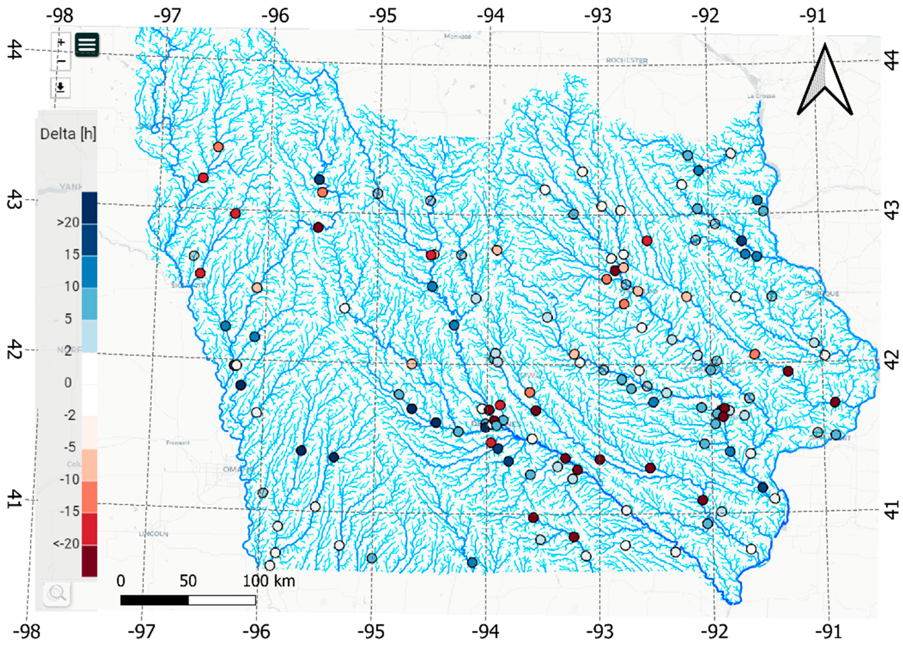
Forecasts produced by the HLM are shared with the National Weather Service. Although, we have succeeded at predicting the magnitude of the peak flow for multiple events (including predicting the 2016 flood in Eastern Iowa with KGE (Kling Gupta efficiency) values between 0.40 and 0.75), predicting the timing of the crest has proven challenging. Figure 1 shows the average time difference between the observed and forecasted time of arrival of the flood crest (peak flow) at 120 gauged locations in Iowa between 2008 and 2018. Our hydrological model relies on a major simplification of the routing equation [13] originally developed to test scaling theories in floods. The formula simplifies routing in the river network as a single equation with three parameters assumed as constant for the Iowa Water Domain. Coupled with radar and meteorological forecasts, the simplification allows updating predictions for the state every 15 minutes for 20 days ahead of time horizon [14,15].
In principle, modeling distributed flows in a river network would require solving a system of partial differential equations (e.g., Saint-Venant Equations, 2D-diffussive wave) which requires prescribing high-resolution hydraulic geometry, including riverbed bathymetries, and local drag coefficients, which would require millions of parameters to be prescribed in the model. Thus, it is surprising that the simplifications of the routing equation (non-linear reservoir) with only three parameters captures all major streamflow fluctuations (including major floods) across multiple spatial scales [14]. For all its value, the simplification leads to limits in predictability of the correct time of arrival of the flood crest, and its magnitude.
The simplification of routing equations relies on the existence of scaling laws in hydraulic geometry [17] which has been observed in data sets around the world. Typically, hydraulic geometric datasets that are used to determine scaling parameters are sparse and cover small geographical extents [17,18,19,20,21,22,23,24] because they are obtained through field surveys. This limitation precludes the possibility of proving a generalization about the universality of the scaling relations.
We aim to understand if an assumption of local self-similarity in Hydraulic Geometry, in contrast to the currently assumed global self-similarity, yields the kind of errors that are common occurrence in the HLM. Local self-similarity is an attractive assumption for model parameterization as it would increase the number of parameters by a factor of thousands instead of by a factor of millions. We define local self-similarity in Hydraulic Geometry as the existence of invariance of the rescaled distribution of hydraulic geometric measures such as channel width, slope, and friction, with different scaling parameters for different sub-catchments within a larger watershed. In contrast, the global self-similar assumption implies that all regions within the watershed obey the same scaling laws.
We use high-quality precipitation fields (Stage IV [25]) to test the predictability of flood peaks and time to peak in the South Skunk basin using the operational configuration of the HLM model. A virtual catchment is created using the local self-similarity concept to define its hydraulic geometry (38 regions, 114 parameters). We then attempt to predict model generated streamflow fluctuations from the virtual watershed using a global-similarity model (1 region, 3 parameters). We aim to determine if the type of errors that result from trying to predict a local self-similar world using a global self-similar model are in the same order of magnitude and follow similar patterns to those observed in the operational setting. Our work is a first step needed to determine the gains in precision that can be expected from a more accurate prescription of regional scaling parameters for Hydraulic Geometric variables.
The paper is organized as follows. In Section 2, we describe the preliminaries and background, in Section 3 we describe our methodology, which includes the setup of the local self-similarity setup, the comparison scenarios, and the HLM setup. In Section 4 we present our results and we discuss about them. Finally, in Section 5 we present our conclusions.
2. Preliminaries
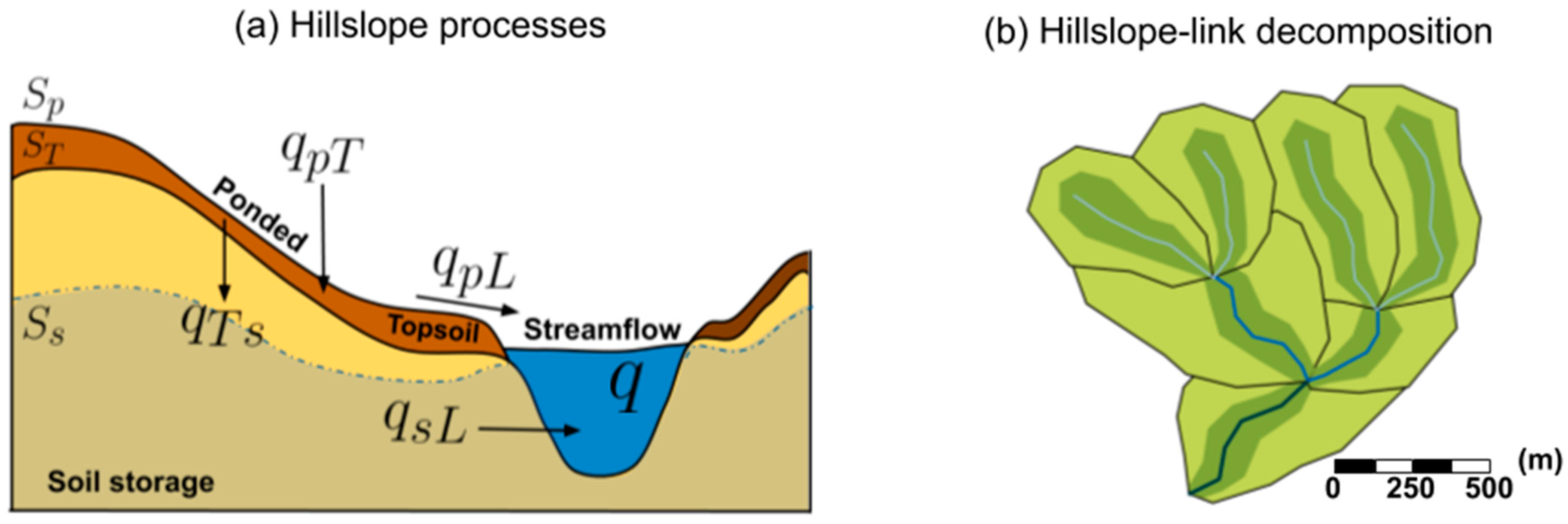
HLM solves the rainfall-runoff partitioning (see Figure 2a) at the hillslope scale and solves the streamflow routing in the channels (see Figure 2b) using an ODE (Ordinary differential equation). The rainfall-runoff partition depends on the interaction between the ponded, topsoil, and soil storages (, , and , respectively). The streamflow routing depends on the mas transport and the routing equations. The mass transport (Equation (1)) relies on the flow velocity (), the channel link length (), the hillslope area (), the upstream streamflow (), and the hillslope ponded and subsurface fluxes ( and , respectively). Channel routing (Equation (2)) relies on calculating flow velocity (), which depends on the streamflow , the link upstream area and three local parameters.
The parameters represent the systematic change in hydraulic geometry properties. They are the reference speed , the streamflow exponent , and the upstream area exponent . According to field data, the value of , , and could vary across watersheds and sub-watersheds [26]. However, it would be very difficult (if not impossible in some cases) to determine their value for all the channels in the river network, thus average parameters are used for the entire river network. This implies an assumption of global self-similarity in the hydraulic geometry [14].
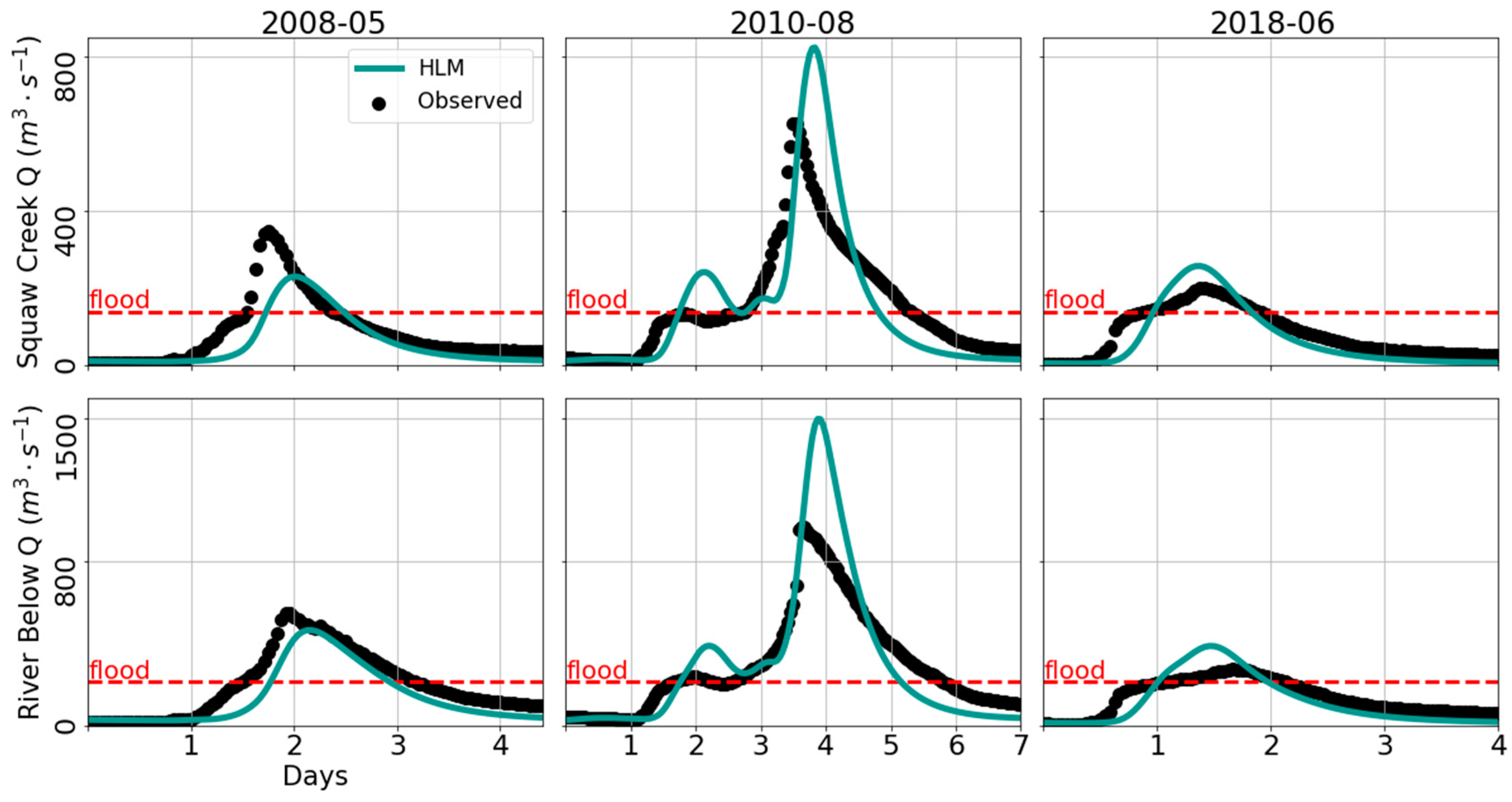
Under the assumption of global self-similarity, the HLM performance can change from one event to the next. For example, using the constant parameters of and the HLM gives variations in its performance at the South Skunk watershed (Figure 3). According to Figure 4, there is variability at the peak flow difference, and at the time to peak. The model predicted a late arrival of the flood crest in the 2008 event and under-estimated the peak flow. On the other hand, it overestimated the peak flow and the time to peak in the event of 2010. Finally, for the 2018 event, the model predicted an early arrival of the peak flow.
In Figure 4, we illustrate three cases; however, we found more variability in the errors when we look at multiple events. In Figure 5a, we compare the scaled peak flows recorded at both stations between 2002 and 2018. We scale both observed () and HLM peak flows () with the observed mean annual peak flow (). With some dispersion, the results show that under the current parameters the model tends to overestimate high peak flows. Moreover, it seems that the dispersion increases with the magnitude of the peak. On the other hand, there is a significant variability at the time to peak difference () with trends around late peak flows forecasts (Figure 5b). In this case, it is uncertain if the errors were only due to the assumption of constant streamflow routing parameters and . However, previous results reinforce our idea that the distribution of both parameters have a significant influence regarding the peak flows ([26,27]).
In this case, we suspect that the distribution of the routing parameters is responsible for a significant portion of the observed errors. However, there are multiple sources of error when we compare simulations with observations [28,29,30,31]. On the model side, these sources of error could be due to the initial conditions [9], parameters [28,32,33], and formulations. On the data side, the sources are related to the rainfall [34,35], and the streamflow observations [36,37]. All these different sources of error make it difficult to identify the relevance of the streamflow routing parameters when comparing modeling results with observations. However, under some assumptions, it is possible to analyze the routing parameter’s importance.
3. Methodology
Our experiment consists of comparing the HLM hydrograph simulations under five different scenarios. One scenario with distributed routing parameters, three scenarios with constant parameters, and one with distributed parameters and noisy rainfall field. The scenario with distributed and and without noise on the rainfall is considered as “observations” or reference. The rainfall-noise scenario and the global self-similarity scenarios represent two different sources of uncertainty.
3.1. Study Catchment and Reference Scenario
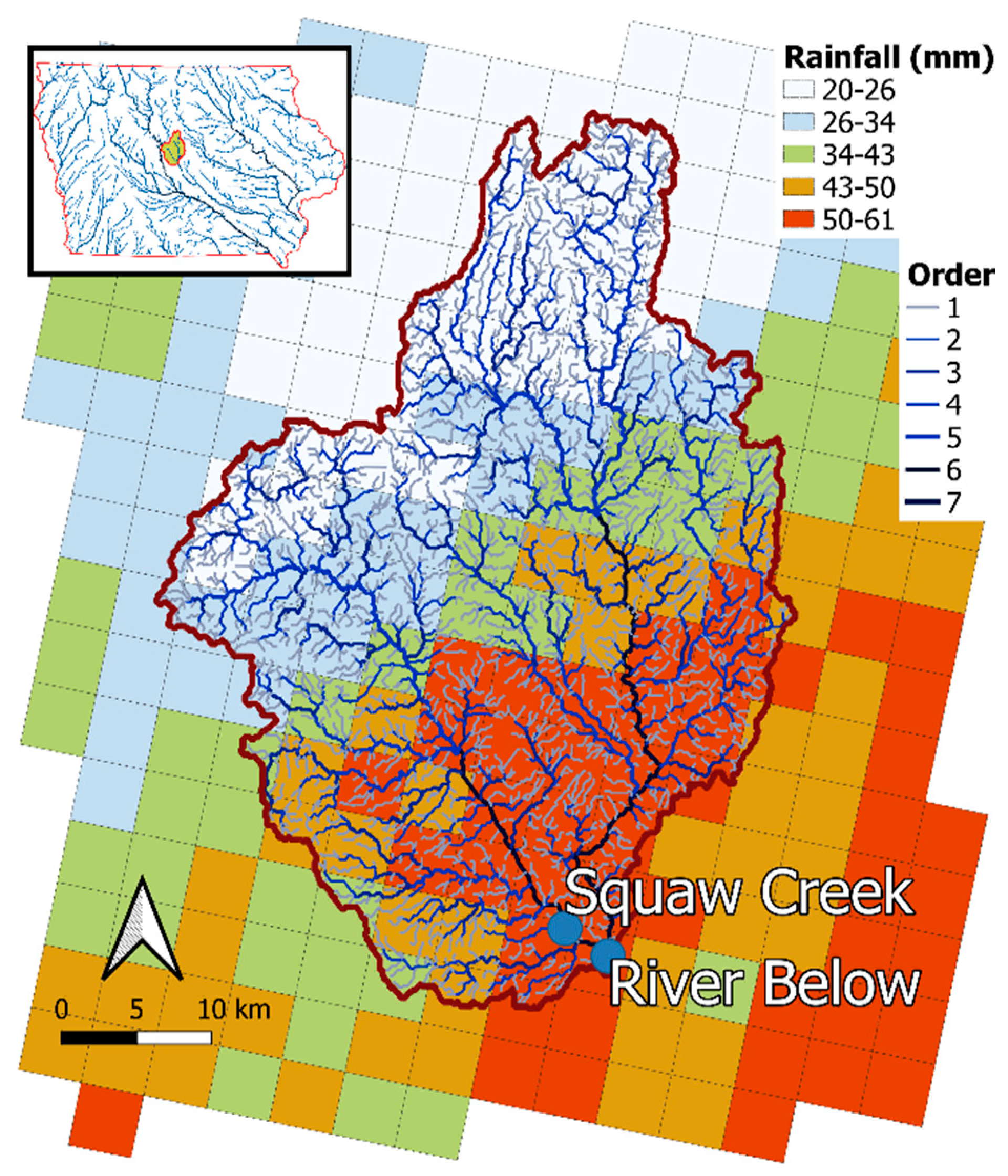
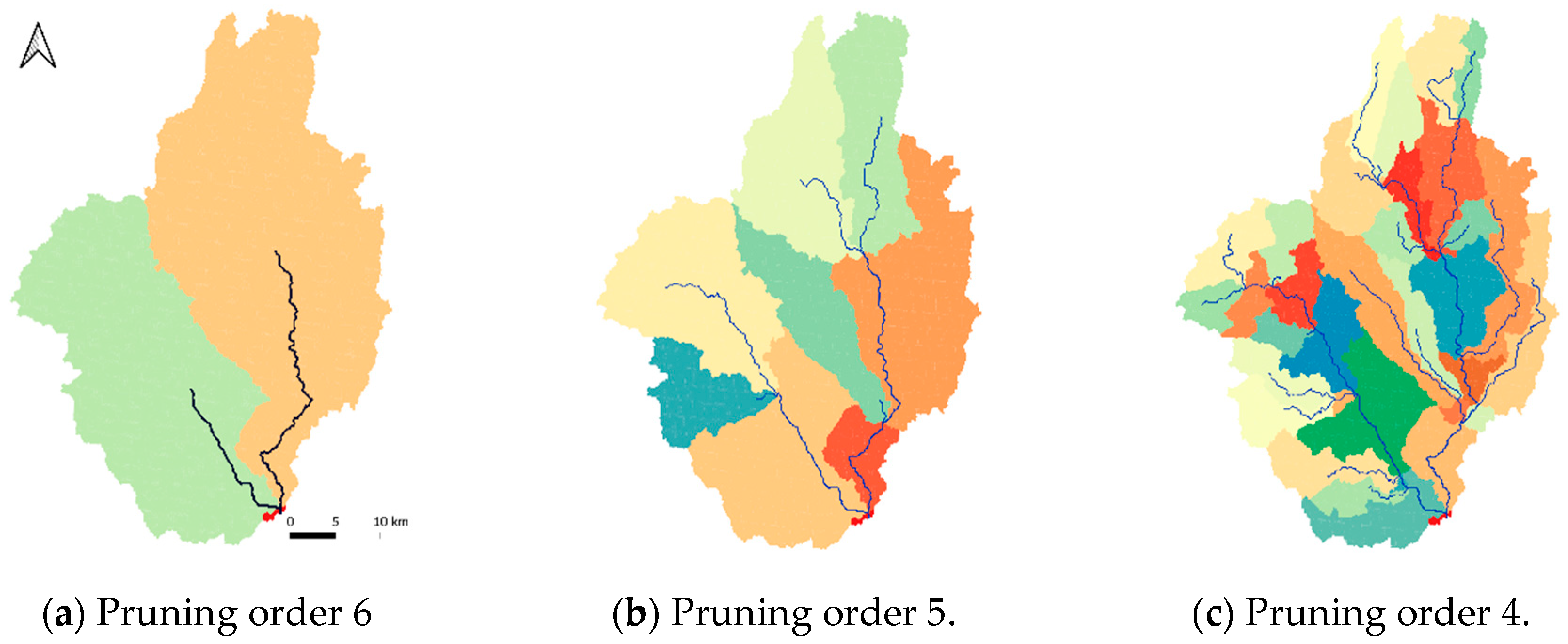
For the experiment we use the South Skunk watershed (Figure 3) which has a total area of 1457 . For the delineation of the watershed and its streamflow network, we use a DTM (Digital terrain model) of 90 [38]. The watershed contains a total of 3201 hillslopes and links, with a mean area of 0.5 and Horton-Strahler [39,40] orders ranging between 1 and 7 (network on Figure 3). To obtain a realistic representation of the streamflow parameters distribution over the space, we divide the watershed into sub-hillslopes. The sub-hillslopes are defined as the area draining to a channel of specific Horton order or higher. For example, if we only consider channels order 6 or higher, we will obtain three main channels, two of order 6 and one order 7 (Figure 6a). If we select order 5 or greater, we obtain nine smaller sub-hillslopes (Figure 6b). Finally, if we consider channels order 4 or higher, we get 38 sub-hillslopes (Figure 6c) with areas of about 50 . For our setup we choose the distribution presented on Figure 6c since it increases the local homogeneity. Moreover, this distribution has a mean sub-hillslope area of 40 , which is usually smaller than the typical area of a deep convective cell in the region [41,42].
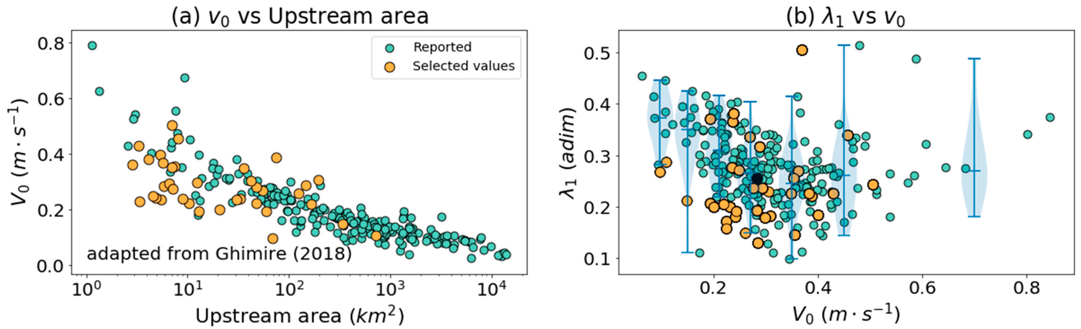
Once we define the units to distribute the parameters, we proceed to assign and . To choose the magnitude of the parameters, we use the values reported by [26]. We transform the results obtained by [26], since they reported values for as a function of the upstream area assuming that equal to 0. To produce the transformation, we multiply the reported values of by (Figure 7a). Which implies assuming . Then for each sub-hillslope, we randomly choose the values of in function of their maximum upstream areas. For this, we divide the records of Figure 7a by taking upstream area intervals following powers of 10. From the same data, we also found that has a decrease tendency for values between 0.1 and 0.3, and tends to increase when is above 0.3 (Figure 7b). Following the described trend, we randomly select in function of the value selected for . With this procedure we aim to obtain a realistic spatial representation of the streamflow routing at the scale of the sub-hillslopes.
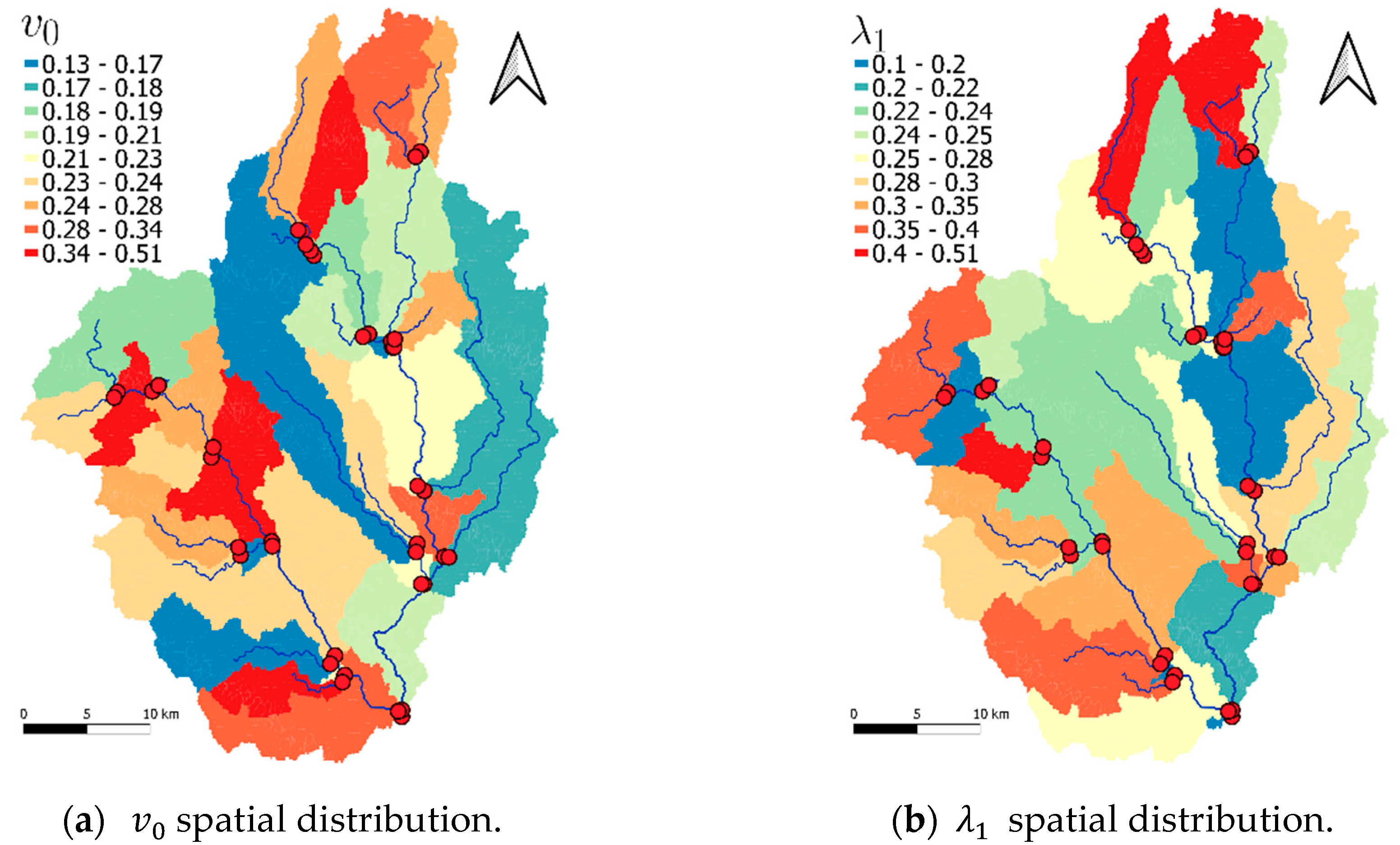
Following the described procedure, we obtain a spatial representation for and , (Figure 8 a and b respectively). This representation is our self-similarity setup in which we assume that and are constant inside each sub-watershed. Additionally, we place control points at the outlet of each sub-hillslope (red dots in Figure 8).
3.2. Comparison Scenarios
As mentioned before, we setup four scenarios to represent two different sources of uncertainty. One scenario considers the local self-similarity setup and includes noise on the rainfall input. The other three scenarios assume global self-similarity without noise at the rainfall. For the noise scenario, we modify the rainfall with a multiplicative factor that has an occurrence probability of 90% when the rainfall is above 1mm. The multiplicative factor comes from a normal distribution with the mean equal to 1 and the standard deviation equal to 0.2. Under this setup, the 90% of the noise produce an error below 30%. On the other hand, the global self-similarity scenarios correspond to the weighted mean, the 25th, and the 75th percentile of the routing parameters. In Table 1 we present the global values corresponding to each global self-similarity setup.
Considering the constant setups, and the noise setup, there is an error relative to the parameters and to the input. In Figure 9, we contrast the noise error with the global setup error. The routing parameters estimation error corresponds to the distribution of the ratio between the assumed constant value and the values distributed for all the elements through the sub-hillslopes (local self-similarity scenario). Each parameter and each setup have a different error distribution. With a trend towards values between 0.5 and 1.0, the P25 setup tends to underestimate both parameters (Figure 9a,b). The mean setup, tends to diminish the errors (Figure 9c,b), and the P75 setup, produces overestimation errors (Figure 9e,f). Despite the differences at the distribution, the four scenarios produce errors of the same order of magnitude.
3.3. Hydrological Modeling Setup
After defining the reference and comparison scenarios, we setup HLM. We run all the cases with Stage IV rainfall between 2002 and 2018 with a time step of 1 h. For all the cases the evaporation corresponds to the monthly mean evapotranspiration recorded by MODIS (Moderate Resolution Imaging Spectroradiometer [43]) between 2008 and 2018. Since the model does not consider snow melt, we run each year from March to December. We use the same and constant hydrological parameters for the five setups, except for the routing parameters at the global self-similarity cases. The hydrological parameters correspond to the ones reported on [14].
4. Results and Discussion
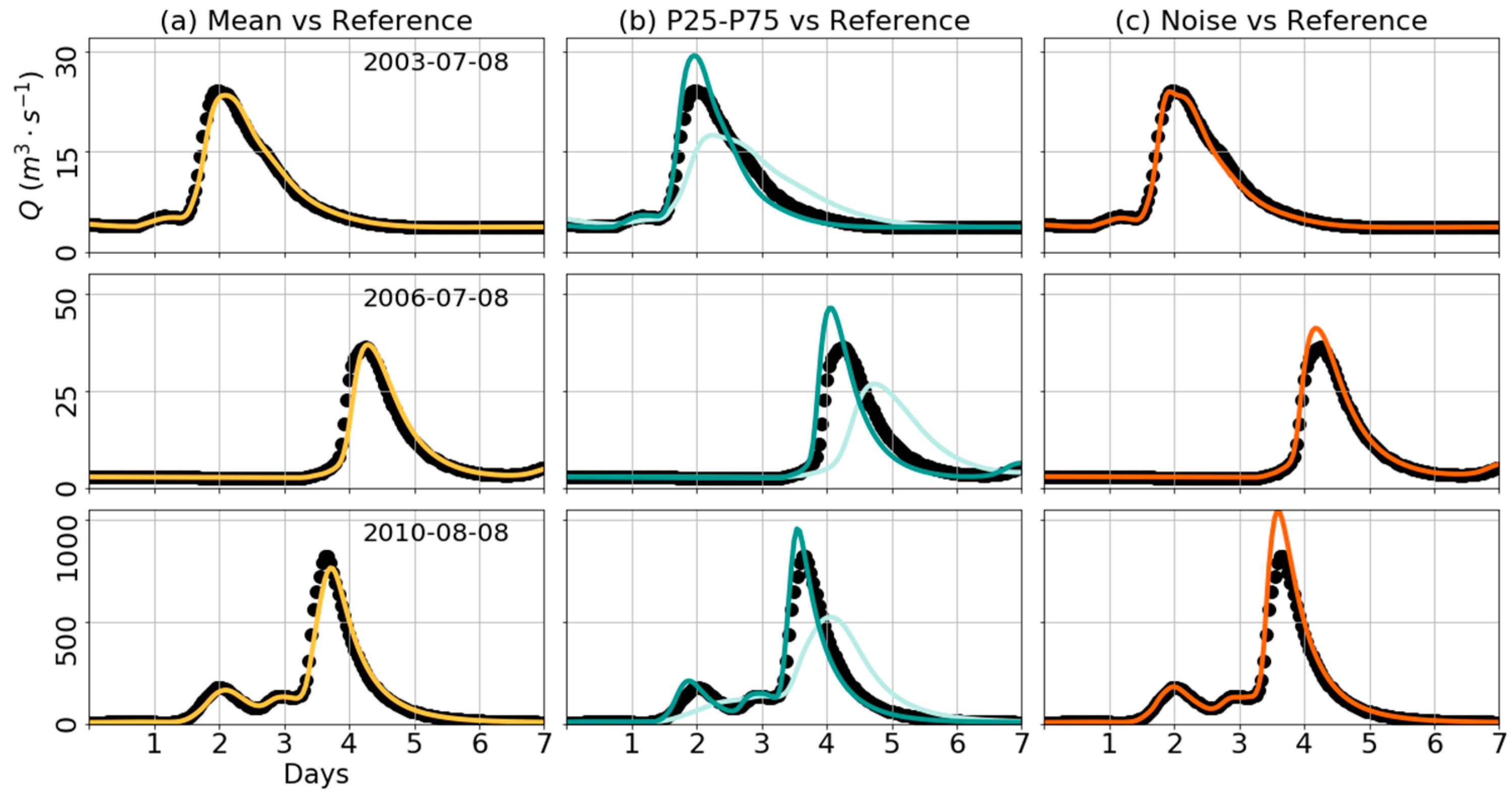
We run the setups described at Table 1 and obtain around 8800 simulated events. For each event we compare the simulated hydrographs with those calculated for the reference setup at the established control points. As an example, in Figure 10 we present the obtained hydrographs at the outlet of the South Skunk watershed for three events. In these cases, the P25 and P75 scenarios exhibit the major differences with the reference setup. On the other hand, the Mean and Noise scenario show a good approximation to the reference. However, these results correspond only to three events at the outlet of the watershed and we require more analysis over the obtained results.
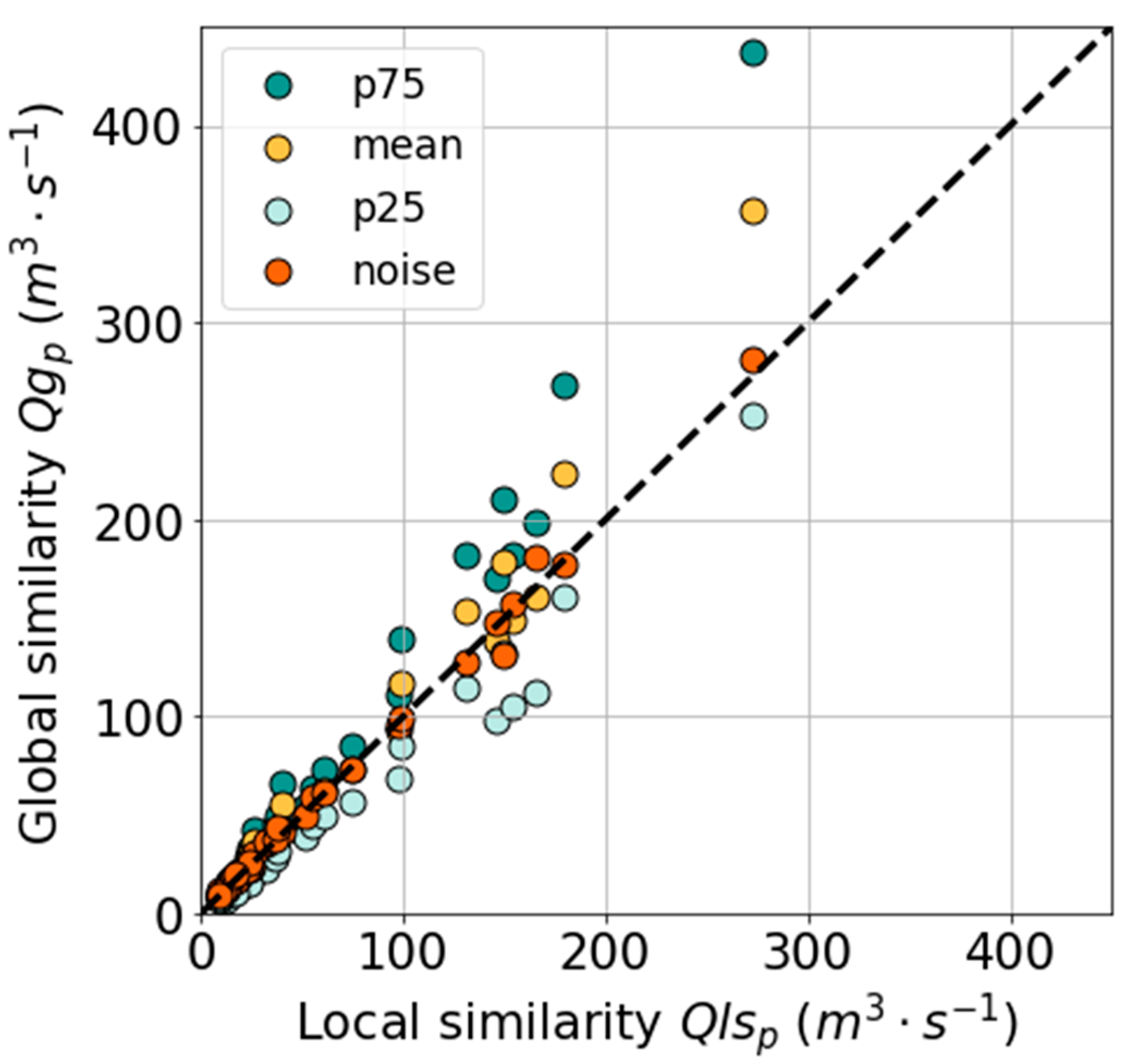
In Figure 11 we compare the mean annual peak obtained with the Global self-similarity setups and the Noise setup. In the figure each point corresponds to a control point located at the outlet of each sub-hillslope. According to it, the Global self-similarity setups overestimate or underestimate the mean annual peak flow. Among the Global setups, the P25 setup is the most accurate, but tends to produce under estimations. On the other hand, the weighted mean setup, tends to be accurate at the upper region of the watershed, however, it overestimates near the outlet. The P75 setup tends to produce overestimations for all the control points. Alternatively, the Noise setup tend to have the most accurate representation of the mean annual peak flows. Since here we compare the mean annual peak flow at each control point, this result describes an overall behavior of each setup. However, it summarizes the effect of assuming constant routing parameters and the potential effect of the noise at the rainfall.
The differences at the mean annual peak flows (Figure 11) coincide at some extent with the error distribution of the parameters (Figure 9). At the global self-similarity scenarios, the error at the mean annual peak flows coincide with the magnitude of the errors produced at the parameter’s estimation. For example, in the P25 setup the error at and is around 0.84, and the mean annual peak flow ratio (error) is around 0.81. In the mean case, the parameters errors are around 1.07, and the mean annual peak flow error is around 1.03. In the P75 case the parameters errors are around 1.25 and the mean error at the annual peak is 1.2. On the other hand, the Noise scenario produce a mean annual peak error of 1.05. The errors produced by the Global and Noise setups are due to different process on the model. The first, is the result of differences at the channels transit speed, while the second, is produced by temporal differences in the total rainfall volume. Despite this difference, it seems that on the long run potential errors at the rainfall measurements are less relevant than the errors derived from the routing parameters.
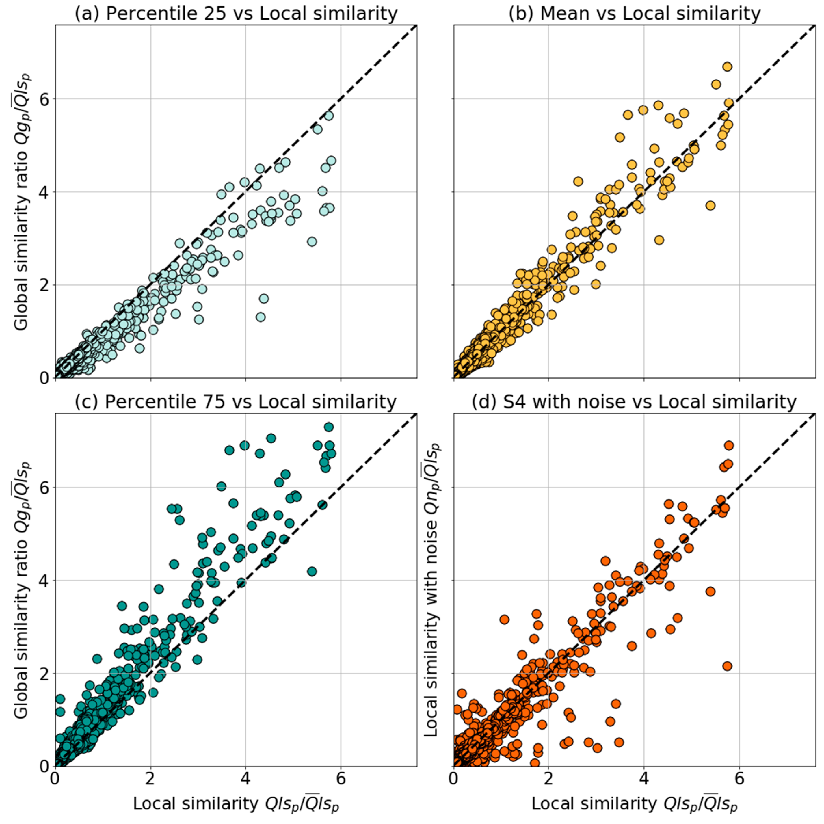
The described averaged behavior becomes disperse when we look at the differences produced at each event (Figure 12). In this case, each setup exhibit a dispersion at the peak flows, but keeps the trend presented in Figure 11. For the P25 scenario the higher under estimations occurs for peak flow between 4 and 6 times the annual mean peak flow (Figure 12a). Alternatively, the Mean and P75 scenarios have under and over estimations (Figure 12b and Figure 12c respectively). However, the higher peak differences are at the P25 and P75 scenarios. According to the results, the peak flow errors increase with the parameters estimation errors and the magnitude of the storm event.
The Global self-similarity cases (Figure 12a–c) have more variability than the Noise case (Figure 12d). Unlike the Global cases, at the Noise case, the dispersion does not increase with the magnitude of the event. The increase of the error at the Global cases could be linked to the spatial localization of the rainfall at each event. From event to event, the rainfall activates different channels of the watershed, which depending on their characteristics will give a determined shape to the hydrograph and eventually to the peak flow. Due to this, there are chances for an event to produce a similar peak flow for the Local and Global self-similarity setups. However, there are also changes to obtain different peak flows when the rainfall falls in regions that have significant differences at the routing parameters. Additionally, our results suggest that at intense events this error could increase significantly. This is an hypothesis that we derive from the results of Figure 12, however, it must be analyzed in detail contrasting the rainfall and the spatial distribution of the routing parameters.
The peak flow differences magnitudes of the observations (Figure 5) and of the virtual setups (Figure 12) are similar. Despite the limited number of events, both cases oscillate around the same order of magnitude respect to the mean annual peak flow. Also, there are similitudes on the overestimation trend obtained with the P75 scenario (Figure 12c). Additionally, the Noise case (Figure 12d) exhibit some of the dispersion observed when comparing HLM with the USGS stations. As mentioned before, the errors observed on Figure 5 are the result of more processes. However, our results suggest that a relevant portion of the errors on the peak flow estimation are the result of differences at the real routing parameters.
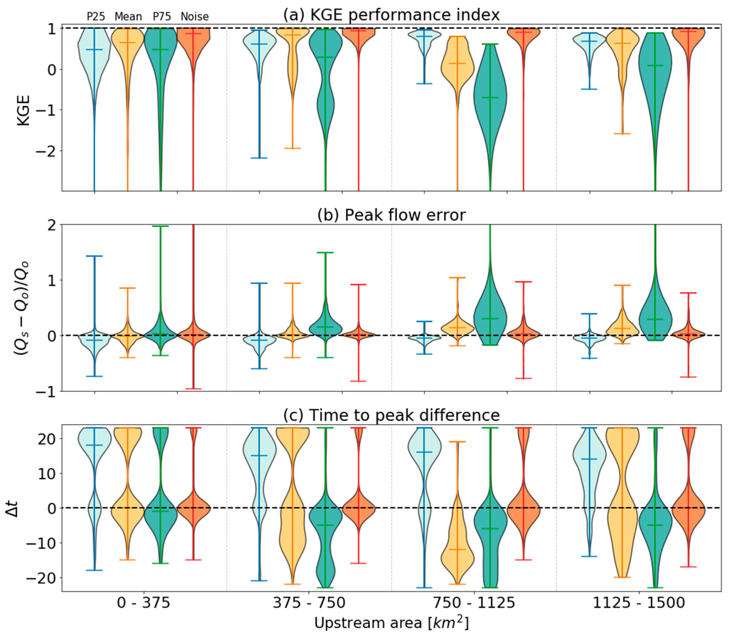
Moreover, routing parameters errors also change the performance across scales. In Figure 13 we show the distribution of the KGE [44], the peak flow ratio, and the time to peak difference by intervals of upstream area. The Noise scenario has the best performance for the three performance indexes, and for all the scales. Also, the error induced by the noise on the rainfall is scale independent. Conversely, for some Global scenarios, the performance seems to be dependent on the scale. This is the case of the Mean and P75 scenarios, in which the KGE and the peak flow ratio decreases their performance with the upstream area. On the contrary, the P25 scenario exhibits a similar KGE and a peak flow ratio across scales. This result suggests that having underestimations at the routing parameters could benefit some performance indexes. However, as shown on Figure 12a, this scenario tends to underestimate the peak flows and the time to peak (Figure 13c).
The time to peak difference change with the scale, and the scenario (Figure 13c). Conversely to the KGE and peak flow differences, the P25 scenario are among the worst cases in terms of this metric. It is the only scenario that produces late peaks at all the scales, with low chances to obtain time to peak errors near zero. On the other hand, the Mean scenario shifts between early and late peak flows, and the P75 scenario tends to produce early peak flows for almost all the cases. Additionally, regardless of the scenario, the time to peak difference, and the peak flow ratio difference tends to improve at the control points with low upstream area (0–375 ).
Considering the performance metrics of Figure 13, the Global setups produce the lower dispersion and the best performance at the control points with lower area. This may be the result of increasing routing parameter errors due to increases at the affected area. Moreover, the affected area could oscillate in function of the size of the storm event and the upstream area of the analyzed channel.
5. Conclusions
This study illustrates the influence of the streamflow routing parameters on the peak flow magnitude and timing. To quantify this influence, we compare the HLM results at multiple storm events considering five different modeling scenarios. Our reference scenario consists on a virtual distribution of the routing parameters of the HLM model following the idea of local self-similarity. To define the local self-similarity, we split a watershed in its sub-hillslopes using the channels of Horton order or greater. Then, we randomly assign the streamflow routing parameters to each sub-hillslope following the values previously reported by [26]. Three scenarios represent potential global self-similarity approximations. In these scenarios, we apply constant routing parameters taking as values the Mean, the 25th, and the 75th percentile of the values assigned in the reference scenario. The last scenario corresponds to the reference case plus noise on the rainfall input. By defining 37 control points inside of the watershed, we compare the global and the noise scenarios with the reference scenario.
The results derived from the Mean scenario show that the global self-similarity approach could lead to an overall good performance. However, its performance from event to event will be variable in function of the real heterogeneity of the parameters. Moreover, the performance of constant values used at real life cases will be constrained by the characteristics of the channels of the watershed.
We also found that slight differences in the parameters of the global self-similarity approach can lead to representative differences at the overall performance of the model. Depending on the parameters we can obtain a model that tends towards underestimation or overestimation of the peak flows. The same result applies for the peak flow timing.
Our results suggest that the error on the streamflow parameters estimation is more relevant than the noise on the rainfall. We highlight this result considering that both errors have a similar order of magnitude, and that the Global scenarios tend to produce higher errors forecasting the peak magnitude and the time to peak. Considering this result, and the actual quality of radar rainfall products such as Stage IV, we think that it is possible to use rainfall and streamflow data to solve the inverse problem to determine the streamflow parameters for HLM or similar hydrological models.
Author Contributions
Conceptualization, Methodology and Writing; N.V. and R.M. Data preparation and figures elaboration; N.V. All authors have read and agreed to the published version of the manuscript.
Funding
This research was funded by MID-America Transportation center, grant number 69A3551747107.
Acknowledgments
The authors would like to thank the IIHR lab and the University of Iowa for the equipment and software support.
Conflicts of Interest
The authors declare no conflict of interest.
References
- Krajewski, W.F.; Smith, J.A. Radar hydrology: Rainfall estimation. Adv. Water Resour. 2002, 25, 1387–1394. [Google Scholar] [CrossRef]
- Berne, A.; Krajewski, W.F. Radar for hydrology: Unfulfilled promise or unrecognized potential? Adv. Water Resour. 2013, 51, 357–366. [Google Scholar] [CrossRef]
- Thomas, E.; Karsten, A.-N.; Claudia, G.; Niels, -E.J.; Markus, Q.; Guido, V.; Baxter, V. Towards a roadmap for use of radar rainfall data in urban drainage. J. Hydrol. 2004, 299, 186–202. [Google Scholar] [CrossRef]
- Wood, E.F.; Roundy, J.K.; Troy, T.J.; Van Beek, L.P.H.; Bierkens, M.F.; Blyth, E.; de Roo, A.; Döll, P.; Mike, E.; James, F. Hyperresolution global land surface modeling: Meeting a grand challenge for monitoring Earth’s terrestrial water. Water Resour. Res. 2011, 47, 1–10. [Google Scholar] [CrossRef]
- Carpenter, T.M.; Georgakakos, K.P.; Sperfslagea, J.A. On the parametric and NEXRAD-radar sensitivities of a distributed hydrologic model suitable for operational use. J. Hydrol. 2001, 253, 169–193. [Google Scholar] [CrossRef]
- Cole, S.J.; Moore, R.J. Distributed hydrological modelling using weather radar in gauged and ungauged basins. Adv. Water Resour. 2009, 32, 1107–1120. [Google Scholar] [CrossRef] [Green Version]
- Thorndahl, S.; Einfalt, T.; Willems, P.; Nielsen, J.E.; ten Veldhuis, M.-C.; Arnbjerg-Nielsen, K.; Rasmussen, M.R.; Molnar, P. Weather radar rainfall data in urban hydrology. Hydrol. Earth Syst. Sci. 2017, 21, 1359–1380. [Google Scholar] [CrossRef] [Green Version]
- Grimaldi, S.; Schumann, G.J.-P.; Shokri, A.; Walker, J.P.; Pauwels, V.R.N. Challenges, opportunities, and pitfalls for global coupled hydrologic-hydraulic modeling of floods. Water Resour. Res. 2019, 55, 5277–5300. [Google Scholar] [CrossRef] [Green Version]
- Pathiraja, S.; Westra, S.; Sharma, A. Why continuous simulation? The role of antecedent moisture in design flood estimation. Water Resour. Res. 2012, 48. [Google Scholar] [CrossRef] [Green Version]
- Bates, P.D.; Neal, J.; Sampson, C.; Smith, A.; Trigg, M. Chapter 9-progress toward hyperresolution models of global flood hazard. In Risk Modeling for Hazards and Disasters; Michel, G., Ed.; Elsevier: Amsterdam, The Nederlands, 2018; pp. 211–232. [Google Scholar]
- Mantilla, R.; Gupta, V.K. A GIS numerical framework to study the process basis of scaling statistics in river networks. IEEE Geosci. Remote. Sens. Lett. 2005, 2, 404–408. [Google Scholar] [CrossRef]
- Gupta, V.K.; Waymire, E.C. Spatial variability and scale invariance in hydrologic regionalization. In Scale Dependence and Scale Invariance in Hydrology; Sposito, G., Ed.; Cambridge University Press: Cambridge, UK, 1998; pp. 88–135. [Google Scholar]
- Mantilla, R. Physical Basis of Statistical Scaling in Peak Flows and Stream Flow Hydrographs for Topologic and Spatially Embedded Random Self-similar Channel Networks; University of Colorado at Boulder: Boulder, CO, USA, 2007. [Google Scholar]
- Quintero, F.; Krajewski, W.F.; Seo, B.C.; Mantilla, R. Improvement and evaluation of the Iowa Flood Center Hillslope Link Model (HLM) by calibration-free approach. J. Hydrol. 2020, 584, 124686. [Google Scholar] [CrossRef]
- Quintero, F.; Krajewski, W.F.; Mantilla, R.; Small, S.; Seo, B.C. A spatial-dynamical framework for evaluation of satellite rainfall products for flood prediction. J. Hydrometeorol. 2016, 17, 2137–2154. [Google Scholar] [CrossRef]
- Jadidoleslam, N.; Goska, R.; Mantilla, R.; Krajewski, W.F. Hydrovise: A non-proprietary open-source software for hydrologic model and data visualization and evaluation. Environ. Model. Softw. 2020. Sumbbited. [Google Scholar]
- Leopold, L.B.; Maddock, T.J. The Hydraulic Geometry of Stream Channels and Some Physiographic Implications (USGS Numbered Series No. 252); US Government Printing Office: Washington, DC, USA, 1953. [Google Scholar]
- Ibbitt, R.P. Evaluation of optimal channel network and river basin heterogeneity concepts using measured flow and channel properties. J. Hydrol. 1997, 196, 119–138. [Google Scholar] [CrossRef]
- Ibbitt, R.P.; McKerchar, A.I.; Duncan, M.J. Taieri river data to test channel network and river basin heterogeneity concepts. Water Resour. Res. 1998, 34, 2085–2088. [Google Scholar] [CrossRef]
- Ibbitt, R.P.; Willgoose, G.R.; Duncan, M.J. Channel network simulation models compared with data from the Ashley River, New Zealand. Water Resour. Res. 1999, 35, 3875–3890. [Google Scholar] [CrossRef]
- Pitlick, J.; Cress, R. Downstream changes in the channel geometry of a large gravel bed river. Water Resour. Res. 2002, 38, 11–34. [Google Scholar] [CrossRef]
- Parker, G.; Wilcock, P.R.; Paola, C.; Dietrich, W.E.; Pitlick, J. Physical basis for quasi-universal relations describing bankfull hydraulic geometry of single-thread gravel bed rivers. J. Geophys. Res. Earth Surf. 2007, 112. [Google Scholar] [CrossRef]
- Palutikof, J.P.; Street, B.R.; Gardiner, E.P. Decision support platforms for climate change adaptation: An overview and introduction. Clim. Chang. 2019, 153, 459–476. [Google Scholar] [CrossRef] [Green Version]
- Wohl, E. 9.1 treatise on fluvial geomorphology. In Treatise on Geomorphology; Shroder, J.F., Ed.; Academic Press: San Diego, CA, USA, 2013; pp. 1–5. [Google Scholar]
- GCIP/EOP Surface: Precipitation NCEP/EMC 4KM Gridded Data (GRIB) Stage IV Data. Available online: https://doi.org/10.5065/D6PG1QDD (accessed on 15 July 2020).
- Ghimire, G.R.; Krajewski, W.F.; Mantilla, R. A power law model for river flow velocity in Iowa Basins. J. Am. Water Resour. Assoc. 2018, 54, 1055–1067. [Google Scholar] [CrossRef]
- Velasquez, N.; Mantilla, R.I.; Krajewski, W.; Quintero, F. Identifying streamflow routing parameters for the HLM hydrological model in Iowa. J. Hydrol. 2020, in press. [Google Scholar]
- Beven, K. Rainfall-Runoff Modelling: The Primer, 2nd ed.; John Wiley & Sons: Chichester, UK, 2012. [Google Scholar]
- Collier, C.G. Flash flood forecasting: What are the limits of predictability? J. Atmos. Sci. Appl. Meteorol. Phys. Oceanogr. 2007, 133, 3–23. [Google Scholar] [CrossRef]
- Singh, V.P.; Asce, F.; Woolhiser, D.A.; Asce, M. Mathematical modeling of watershed hydrology. J. Hydrol. Eng. 2002, 7, 270–292. [Google Scholar] [CrossRef] [Green Version]
- Vrugt, J.A.; Gupta, H.V.; Bouten, W.; Sorooshian, S. A Shuffled Complex Evolution Metropolis algorithm for optimization and uncertainty assessment of hydrologic model parameters. Water Resour. Res. 2003, 39. [Google Scholar] [CrossRef] [Green Version]
- Rodriguez-Rincon, J.P.; Pedrozo-Acuna, A.; Berena-Naranjo, J. Propagation of hydro-meteorological uncertainty in a model cascade. Hydrol. Earth Syst. Sci. 2015, 19, 2981–2998. [Google Scholar] [CrossRef] [Green Version]
- Mejia, A.I.; Reed, S.M. Evaluating the effects of parameterized cross section shapes and simplified routing with a coupled distributed hydrologic and hydraulic model. J. Hydrol. 2011, 409, 512–524. [Google Scholar] [CrossRef]
- Villarini, G.; Mandapaka, P.V.; Krajewski, W.F.; Moore, R.J. Rainfall and sampling uncertainties: A rain gauge perspective. J. Geophys. Res. Atmos. 2008, 113, 1–12. [Google Scholar] [CrossRef]
- Yang, D.; Koike, T.; Tanizawa, H. Application of a distributed hydrological model and weather radar observations for flood management in the upper Tone River of Japan. Hydrol. Process. 2004, 18, 3119–3132. [Google Scholar] [CrossRef]
- Ibbitt, R.P.; Clark, M.P.; Woods, R.A.; Zheng, X.; Slater, A.G.; Rupp, D.E.; Schmidt, J.; Uddstrom, M. Hydrological data assimilation with the ensemble Kalman filter: Use of streamflow observations to update states in a distributed hydrological model. Adv. Water Resour. 2008, 31, 1309–1324. [Google Scholar] [CrossRef]
- Hamilton, A.S.; Moore, R.D. Quantifying uncertainty in streamflow records. Can. Water Resour. J./Rev. Can. Des. Ressour. Hydr. 2012, 37, 3–21. [Google Scholar] [CrossRef]
- Quintero, F.; Krajewski, W.F. Mapping outlets of iowa flood center and national water center river networks for hydrologic model comparison. J. Am. Water Resour. Assoc. 2018, 54, 28–39. [Google Scholar] [CrossRef]
- Strahler, A.N. Quantitative analysis of watershed geomorphology. Eos Trans. Am. Geophys. Union 1957, 38, 913–920. [Google Scholar] [CrossRef] [Green Version]
- Horton, R.E. Erosional Development of Streams and Their Drainage Basins; Hydrophysical Approach to Quantitative Morphology. GSA Bull. 1945, 56, 275–370. [Google Scholar] [CrossRef] [Green Version]
- Duda, J.D.; Gallus, W.A. Spring and summer midwestern severe weather reports in supercells compared to other morphologies. Weather Forecast. 2010, 25, 190–206. [Google Scholar] [CrossRef] [Green Version]
- Therrell, M.D.; Bialecki, M.B. A multi-century tree-ring record of spring flooding on the Mississippi River. J. Hydrol. 2015, 529, 490–498. [Google Scholar] [CrossRef] [Green Version]
- MODIS/Terra Net Evapotranspiration 8-Day L4 Global 500 m SIN Grid. Available online: https://doi.org/10.5067/MODIS/MOD16A2.006 (accessed on 15 July 2020).
- Gupta, H.V.; Kling, H.; Yilmaz, K.K.; Martinez, G.F. Decomposition of the mean squared error and NSE performance criteria: Implications for improving hydrological modelling. J. Hydrol. 2009, 377, 80–91. [Google Scholar] [CrossRef] [Green Version]
Figure 1.
Averaged time difference between the observed and HLM forecasted time of arrival for 120 USGS (United States Geological Survey) stations for the 2016. Screenshot taken from an HLM evaluation displayed on the Hydrovise web platform [16] (IFC HLM development link: http://visualriver.net/). The averaged time difference is the lag (in hours) on the simulated streamflow that maximizes the correlation with the observations.

Figure 2.
Schematic of the Hillslope Link Model. Hydrological processes occur at the hillslope (a), and routing of the runoff follows the topology of the drainage network (b). Each hillslope drains to a unique channel or link.
Figure 2.
Schematic of the Hillslope Link Model. Hydrological processes occur at the hillslope (a), and routing of the runoff follows the topology of the drainage network (b). Each hillslope drains to a unique channel or link.

Figure 3.
South Skunk watershed (red line) and localization (top panel). The colored squares correspond to a random rainfall event observed by Stage IV, included here to contrast the rainfall resolution with the watershed and its network. The blue dots correspond to three USGS gauge stations of Squaw creek at Ames (05470500), and South skunk River Below Squaw creek (05471000).

Figure 4.
HLM streamflow compared with USGS streamflow records at Squaw Creek (first row) and River Below Squaw Creek (second row). The columns correspond to events observed in May, August, and June of 2008, 2010, and 2018, respectively. The days correspond to the elapsed days since the start of each event.

Figure 5.
Peak flow and time to peak performance of the HLM model at the USGS stations of the South Skunk watershed. (a) Modeled vs. observed peak flow ratios respect to the observed mean annual peak. (b) Time to peak difference () distribution.
Figure 5.
Peak flow and time to peak performance of the HLM model at the USGS stations of the South Skunk watershed. (a) Modeled vs. observed peak flow ratios respect to the observed mean annual peak. (b) Time to peak difference () distribution.

Figure 6.
South Skunk watershed segmentation into sub-hillslopes according to different Horton orders. (a) Selection of sub-hillslopes order 6 that drain to order 7. (b) sub-hillslopes of order 5 that flow to order 6. (c) sub-hillslopes of order 4 that drain to order 5.
Figure 6.
South Skunk watershed segmentation into sub-hillslopes according to different Horton orders. (a) Selection of sub-hillslopes order 6 that drain to order 7. (b) sub-hillslopes of order 5 that flow to order 6. (c) sub-hillslopes of order 4 that drain to order 5.

Figure 7.
Observed streamflow routing parameters for multiple USGS stations at Iowa. (a) vs. the upstream area (adapted from [26]). (b) vs. at the same stations. The green dots correspond to the observations and the orange dots to the randomly selected values for the sub-hillslopes.
Figure 7.
Observed streamflow routing parameters for multiple USGS stations at Iowa. (a) vs. the upstream area (adapted from [26]). (b) vs. at the same stations. The green dots correspond to the observations and the orange dots to the randomly selected values for the sub-hillslopes.

Figure 8.
Local self-similarity spatial distribution of the routing parameters and (a) and (b) respectively.
Figure 8.
Local self-similarity spatial distribution of the routing parameters and (a) and (b) respectively.

Figure 9.
Probability distribution of the ratio between the global and the local self-similarity and parameters (a–f). Values below 1.0 denote underestimation from the global setup, and above, over-estimation.
Figure 9.
Probability distribution of the ratio between the global and the local self-similarity and parameters (a–f). Values below 1.0 denote underestimation from the global setup, and above, over-estimation.

Figure 10.
Simulated hydrographs at the outlet of the watershed. The black dots correspond to the local self-similarity setup (or reference). The results of the comparison setups are divided into columns, column (a) corresponds to the Mean scenario, column (b) to the P25 and P75 scenarios, and column (c) to the Noise scenario.

Figure 11.
Mean annual peak flow of the Global self-similarity and Noise setups vs. the mean annual peak flow of the Local self-similarity setup.
Figure 11.
Mean annual peak flow of the Global self-similarity and Noise setups vs. the mean annual peak flow of the Local self-similarity setup.

Figure 12.
Global self-similarity () and noise scenario peak flows () vs. local self-similarity scenario peak flows (). (a) Case of the P25 scenario, (b) case of the Mean scenario, (c) P75 scenario, and (d) Noise scenario.
Figure 12.
Global self-similarity () and noise scenario peak flows () vs. local self-similarity scenario peak flows (). (a) Case of the P25 scenario, (b) case of the Mean scenario, (c) P75 scenario, and (d) Noise scenario.

Figure 13.
Comparison scenarios performance distribution in function of the upstream area. (a) KGE index, (b) peak flow ratio, and (c) time to peak difference.
Figure 13.
Comparison scenarios performance distribution in function of the upstream area. (a) KGE index, (b) peak flow ratio, and (c) time to peak difference.


Table 1.
HLM setups. HLM setups. In the distributed setups v and λ take the values of the Figure 8a and b, respectively. The Mean, P25, and P75, are derived from the random values assigned to each link of 232 each sub-watershed.
Table 1.
HLM setups. HLM setups. In the distributed setups v and λ take the values of the Figure 8a and b, respectively. The Mean, P25, and P75, are derived from the random values assigned to each link of 232 each sub-watershed.
| and Distribution | Setup Name | Setup Use | Value | Value | Rainfall |
|---|---|---|---|---|---|
| Local self-similarity | Local | Reference | Distributed | Distributed | Stage IV |
| Noise | Comparison | Distributed | Distributed | Stage IV + noise | |
| Global self-similarity | Mean | Comparison | 0.29 | 0.23 | Stage IV |
| P25 | Comparison | 0.23 | 0.18 | Stage IV | |
| P75 | Comparison | 0.34 | 0.27 | Stage IV |
© 2020 by the authors. Licensee MDPI, Basel, Switzerland. This article is an open access article distributed under the terms and conditions of the Creative Commons Attribution (CC BY) license (http://creativecommons.org/licenses/by/4.0/).
Share and Cite
MDPI and ACS Style
Velasquez, N.; Mantilla, R. Limits of Predictability of a Global Self-Similar Routing Model in a Local Self-Similar Environment. Atmosphere 2020, 11, 791. https://doi.org/10.3390/atmos11080791
AMA Style
Velasquez N, Mantilla R. Limits of Predictability of a Global Self-Similar Routing Model in a Local Self-Similar Environment. Atmosphere. 2020; 11(8):791. https://doi.org/10.3390/atmos11080791
Chicago/Turabian StyleVelasquez, Nicolas, and Ricardo Mantilla. 2020. "Limits of Predictability of a Global Self-Similar Routing Model in a Local Self-Similar Environment" Atmosphere 11, no. 8: 791. https://doi.org/10.3390/atmos11080791
Note that from the first issue of 2016, this journal uses article numbers instead of page numbers. See further details here.