Article

An Index for Depicting the Long-Term Variability of Mesoscale Eddy Activity over the Kuroshio Extension Region

1
College of Meteorology and Oceanography, National University of Defense Technology, Nanjing 211101, China
2
State Key Laboratory of Numerical Modeling for Atmospheric Sciences and Geophysical Fluid Dynamics (LASG), Institute of Atmospheric Physic, Chinese Academy of Sciences, Beijing 100029, China
3
College of Earth Science, University of Chinese Academy of Sciences, Beijing 100049, China
*
Authors to whom correspondence should be addressed.
Atmosphere 2020, 11(8), 792; https://doi.org/10.3390/atmos11080792
Submission received: 3 June 2020 / Revised: 13 July 2020 / Accepted: 21 July 2020 / Published: 27 July 2020
(This article belongs to the Special Issue Air-Sea Interaction)

Abstract

:
Using high-resolution satellite-derived sea surface temperature (SST) data from September 1981 to December 2015, the present study develops a new index to detect the long-term variation in mesoscale eddy activity over the Kuroshio Extension (KE) region. This eddy activity index (EAI) highlights the strength of eddy-induced poleward heat transport and has obvious advantages over the other existing KE indices in depicting the low-frequency changes in KE eddy activity. An analysis of the EAI shows that over the long term, the KE eddy activity variability presents a significant spectral peak of about 8 years and is not directly modulated by wind-driven oceanic Rossby waves generated in the central North Pacific. When the EAI is positive, the strengthened KE eddy activity significantly enhances the heat release from ocean to atmosphere over the Kuroshio–Oyashio confluence region (KOCR). This induces an anomalous dipole pattern of near-surface baroclinicity over this region that can persist for up to 6 months, favoring a weakened and northward-moving East Asian jet, and vice versa. It is believed that the new EAI will facilitate future studies focusing on the climatic effects of the KE eddy activity variation.

1. Introduction

Mesoscale oceanic eddies are ubiquitous in the global ocean and account for a large portion of the ocean’s energy [1,2]. These fluctuations efficiently transport heat, salt, energy, and nutrients in the ocean, e.g., [3,4,5]. The Kuroshio Extension (KE) is a region (32°–38° N, 142°–155° E) with the largest eddy kinetic energy (EKE) in the North Pacific (Figure 1a) [6]. In this region, mesoscale eddies can alter the state of the mean current through eddy–mean flow interaction [6,7] and play an important role in the formation of subtropical mode water [8,9]. In addition, KE mesoscale eddies can cause significant local [10,11,12,13] and, even, remote atmospheric responses [14,15,16].
Considering its importance in oceanic general circulation, air–sea interaction, and climate, the main features of KE eddy activity variability deserve to be studied. With the aid of high-quality sea surface height (SSH) data from satellite measurements, researchers have continuously investigated KE mesoscale eddies and found that their EKE shows obvious decadal variation. This variation corresponds well to the strength, position, and path state changes of the KE jet [17]. Specifically, the regional EKE level increases (decreases) when the KE jet is weak (strong) and shifts southward (northward) with a lengthening (shortening) path state. However, it should be noted that satellite-derived SSH data have been available only since October 1992. The limited length of the data may hinder knowledge about the KE eddy activity variability and its climatic effects. Therefore, the goal of the present study is to develop a new index that can describe the long-term behavior of KE eddy activity rather than the conventional EKE index derived from the short-period satellite-derived SSH data.
Some studies have reported that anomalous KE eddy activity alters the poleward heat transport, leading to a change in sea surface temperature (SST) over the Kuroshio–Oyashio confluence region (KOCR; 34°–42° N, 141°–150° E) [18,19]. Inspired by these works, we have constructed the new index of KE eddy activity from its related SST anomalies using high-resolution satellite-derived SST data from Reynolds et al. [20] on a 0.25° × 0.25° grid. The reasons conclude the two aspects. Firstly, the satellite-derived SST product has been available since September 1981, more than 11 years prior to satellite-derived SSH data, which provides a relatively long time series and thus facilitates the investigation of the long-term (i.e., interannual-to-decadal) variability in the KE eddy activity. Secondly, the KE eddy activity impacts the atmosphere through modulating the SST anomalies. Therefore, defining an SST-based index will contribute to understanding the impacts of KE eddy activity variability on ocean–atmosphere interaction and climate.
The remainder of this paper is organized as follows. Section 2 describes the datasets used in this study. Section 3 introduces the new eddy activity index (EAI) and analyses the advantage of this index in comparison to the existing KE indices. Based on the EAI, Section 4 investigates the relationship between the long-term behavior of KE eddy activity and wind-driven oceanic Rossby waves. The impacts of KE eddy activity variation on the air–sea heat flux and near-surface baroclinicity are discussed in Section 5. Conclusions are given in Section 6.

2. Data and Methods

The SST data were obtained from the monthly National Oceanic and Atmospheric Administration (NOAA) optimum interpolation SST (OISST) data product [20] for the period from September 1981 to December 2015, which is based on Advanced Very High-Resolution Radiometer (AVHRR) infrared satellite data and has a high spatial resolution of 0.25°. In addition, the SST, surface air temperature (SAT), and turbulent-heat-flux data from the Objectively Analyzed Air–Sea Fluxes (OAflux) product [21] with a 1° spatial resolution for the same period as OISST were also utilized. For the SSH, two datasets were adopted in the present study: one set contains the daily satellite altimetry data of the Archiving, Validation, and Interpretation of Satellite Oceanographic (AVISO) product [22] on a 0.25° × 0.25° grid for the period from 1 January 1993 to 31 December 2015. The other set consists of the monthly simple ocean data assimilation (SODA) SSH reanalysis product [23] for the period from September 1981 to December 1992, with a horizontal resolution of 0.5° × 0.5°. The atmospheric variables, including SAT, turbulent heat flux, wind stress, and zonal winds obtained from the ERA-Interim reanalysis with a 0.75° grid, were also used [24].
In this study, following the work of Qiu and Chen [17], the high-frequency EKE was calculated based on the high-pass filtered AVISO SSH anomaly data with time scales shorter than 300 days to indicate the strength of mesoscale eddy activity:
EKE = 1 2 [ ( g f h y ) 2 + ( g f h x ) 2 ] ,
where g is the gravitational constant, f is the Coriolis parameter, and h′ is the AVISO SSH anomaly. The mean seasonal cycle for all variables was removed by subtracting the climatological monthly means, and the influences of trends were then also eliminated by least-squares fitting. We assessed the statistical significance of all regression or correlation coefficients between the two-time series based on two-tailed Student’s t-test using the effective number of degrees of freedom, which takes serial autocorrelation into consideration [25].

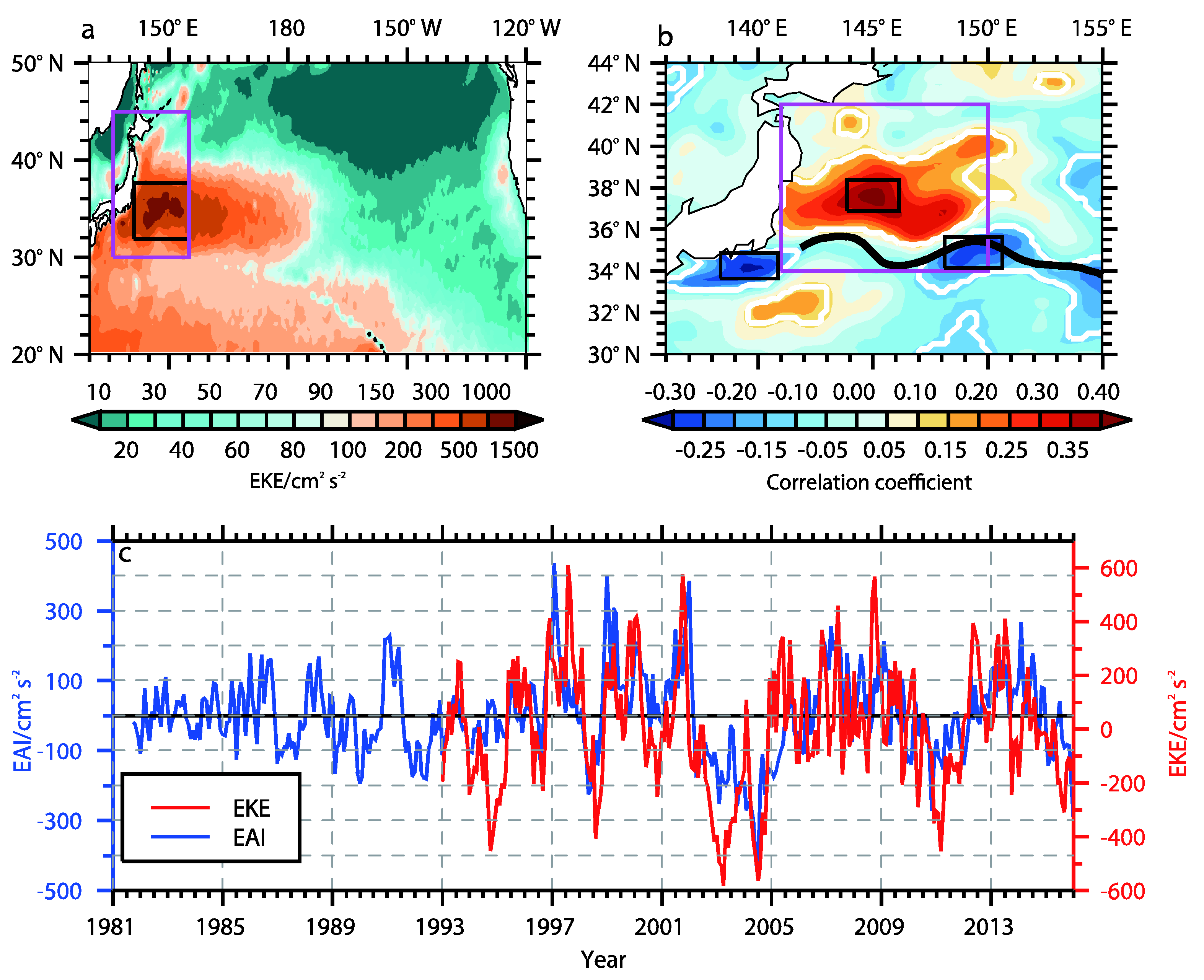
3. The KE Eddy Activity Index

3.1. Definition

Firstly, the imprints of KE eddy activity on the SST are investigated, which provides the basis for the construction of a new EAI. Figure 1b shows the correlation map of the SST anomalies with the EKE time series averaged over the KE region (Figure 1c, red line). The most significant correlations mainly occur in the regions around the KE jet axis: the KE EKE level shows significant positive correlations with the SST anomalies over the central part of KOCR, consistent with the findings of [18,19]. In addition, there are significant negative correlations to the southeast of Japan and around 150° E. These significant positive and negative correlations are located to the northern and southern flanks of the KE jet axis, respectively. This distribution actually reflects the strengthened poleward transport of warm water by the enhanced KE eddy activity. According to Seo et al. [26], when the KE eddy activity is enhanced, more warm water is transported to the north of the KE jet axis, which increases the SST in the north but decreases the SST in the south.
In these regions with significant EKE–SST relationship, it can be further found from Figure 1b that the strongest linear correlations emerge in three subdomains: A (36.875°–38.375° N, 143.875°–146.125° E), B (33.625°–34.875° N, 138.375°–140.875° E), and C (34.125°–35.625° N, 148.125°–150.625° E). On the basis of the above analysis, the EAI can be defined by a multiple linear regression model as follows:
EAI = α T A + β T B + γ T c ,
where TA, TB, and Tc denote the normalized SST anomalies averaged over regions A, B, and C, respectively. The coefficients α, β, and γ are obtained by the least-square method, which quantifies the EKE–SST relationship and gives a 103.98 cm−2 s−2 EKE increase per standard deviation increase in TA, 52.99 cm−2 s−2 EKE decrease per standard deviation increase in TB, and 60.25 cm−2 s−2 EKE decrease per standard deviation increase in TC, respectively. Although the amplitude of new EAI is a little weaker than that of observed KE EKE variation, it can be clearly seen that the two-time series corresponds well during the overlapping period (Figure 1c). The correlation coefficient between them is r = 0.57 with monthly resolution and r = 0.83 with annual resolution, which is significantly high (Table 1). These results imply that the EAI is a good indicator for the low-frequency KE eddy activity variability on interannual and longer time scales.

3.2. Advantage of the New EAI

As mentioned in the introduction, the low-frequency KE eddy activity variability usually co-varies with the indices that detect the changes in strength, position, and pathlength of KE jet. These KE indices are also closely related to the strength of its southern recirculation gyre and can be depicted by another index defined as the area-averaged SSH anomalies over the domain 31°–36° N, 140°–165° E ([27]; the SSH index). The capacity of above KE indices in depicting the low-frequency KE eddy activity variability was compared with that of the new EAI. Following the methods of Seo et al. [26], we deduced the indices of jet strength, path state, and position by detecting the KE SST front because it closely follows the behavior of the KE jet. As shown in Table 1, the existing KE indices are generally significantly correlated with the EKE level, except the jet position. However, the EAI shows the strongest correlation with the EKE variation among all these KE indices. Therefore, the newly defined EAI has a distinct advantage in identifying the low-frequency EKE variation compared with the other existing KE indices.
In order to further understand the advantage of the EAI, a power spectrum analysis was conducted. Surprisingly, this index mainly shows significant oscillations with a period of about 8 years (Figure 2a), which is different with the period of about 10 years in KE jet fluctuations reported by previous studies [26,27,28,29]. Actually, the conventional EKE index also shows the spectral peak of about 8 years, but it is not statistically significant (Figure 2b). This discrepancy may be caused by the short time span of EKE index compared with the EAI. Indeed, the EAI during 1993–2015 shows the insignificant spectral peak of about 8 years as well (figure not shown). Therefore, the long-term period of about 8 years in KE eddy activity identified from the EAI should be robust, which has been overlooked due to the limited length of data. In addition, it was found that among all the existing KE indices, only the jet strength can reproduce this spectral peak of about 8 years (Figure 2c), whereas the other indices present significant periods of about 10 years reported by previous studies (Figure 2d–f). These results indicate that there are obvious deficiencies in existing KE indices for capturing the long-term variation of KE eddy activity and further support the advantages of the new EAI.

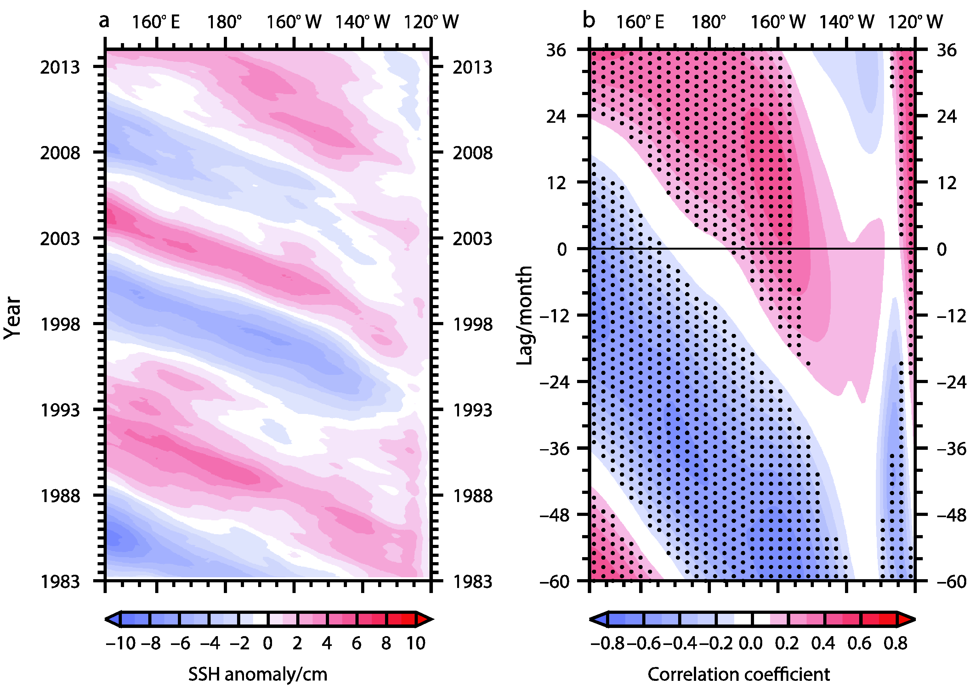
4. Relationship with Oceanic Rossby Waves

As indicated above, the EAI well reveals the characteristics of long-term KE eddy activity variability. However, what drives this oceanic variability needs to be determined. Qiu and Chen [17] indicated that the changes in KE eddy activity result from the KE jet meridional movement over the Izu–Ogasawara Ridge. Specifically, when the KE jet moves southwards and rides over the ridge through a shallow segment, the local perturbations are generated, leading to a strengthened KE eddy activity. On the other hand, the northward-moving KE jet passes through a deep channel, weakening the KE eddy activity. Many previous works have found that the meridional migration of the KE jet is primarily forced by the wind-driven oceanic Rossby waves generated over the central North Pacific, e.g., [6,17,30,31,32]. Therefore, it can be inferred that the long-term KE eddy activity variability should be strongly modulated by the oceanic Rossby waves, which is supported by the results of Yang et al. [33] based on model outputs. Nevertheless, some studies have suggested that the KE eddy activity is associated with the path of the upstream Kuroshio south of Japan rather than with oceanic Rossby waves [26,34]. Furthermore, we also noted that the new EAI shows little correlation with the KE jet meridional shift (Table 1), indicating that the changes in KE eddy activity may not be triggered by the oceanic Rossby waves. Accordingly, the relationship between the KE eddy activity and the wind-driven oceanic Rossby waves remains controversial. This question is discussed in this subsection to advance the understanding of the mechanisms for the long-term KE eddy activity variability.
To detect oceanic Rossby waves over the long term, a 37-month running mean filter was used in SSH anomaly data from merged AVISO satellite data and SODA reanalysis to highlight the low-frequency signals. Figure 3a shows the SSH anomalies averaged over the band from 33°–35° N, where the zonal mean KE axis is located [26]. It is clearly seen that the SSH anomalies originating in the central North Pacific propagate westward into the KE region, indicating the behavior of the oceanic Rossby waves. Then, the relationship between these SSH anomalies and the KEEAI was investigated. As shown in Figure 3b, the EAI shows significant negative correlations with the SSH anomalies formed in the central North Pacific around 180°–160° W at a lead time of 48 to 60 months (4–5 years). These oceanic signals associated with the EAI propagate westward into the KE region at a lead time of 12 months (1 year), indicating that the changes in KE eddy activity variation actually lag the arrival of the oceanic Rossby waves into the KE region by approximately one year. Seo et al. [26] also determined that the KE jet path state change shows a similar delay relative to the arrival of oceanic Rossby waves into the KE region, which supports our findings here.
To further verify the above results, a simple Rossby wave model was adopted. Specifically, under the long-wave approximation, the linear vorticity equation of the model is
h t c R h x = g curl τ ρ 0 g f ,
where h is the SSH anomaly, CR is the speed of the long baroclinic Rossby waves, g is the gravitational constant (9.81 m s−2), g′ is the reduced gravity (0.03 m s−2), ρ 0 is the reference density of seawater (1025 kg m−3), f is the Coriolis parameter, and τ is the anomalous wind-stress vector. The solution for Equation (3) can be obtained by integrating this equation along the baroclinic Rossby wave characteristic:
h ( x , y , t ) = g ρ 0 g f c R 0 x curl τ ( x , y , t + x x c R ) d x .
Using the wind-stress data and Equation (4), we hindcast the h(x,y,t) field for the midlatitude North Pacific. It should be noted that in Equation (4), the solution due to the eastern boundary forcing at x = 0 is ignored according to Fu and Qiu [35]. Figure 4a shows the time–longitude plot of the SSH anomalies from the model outputs over the band of 33°–35° N. Compared with the observation in Figure 3a, the modeled SSH anomalies are spatially smoother because the Equation (4) fails to depict the mesoscale oceanic signals [17]. Moreover, the westward propagation of SSH anomalies in Figure 4a can be traced from the eastern North Pacific, which also differs from that of the central North Pacific in observation. However, the Rossby wave model captures the observed low-frequency SSH changes in the KE region west of 155° E well (e.g., negative SSH anomalies in 1983–1988, 1997–2002, and 2007–2010 and positive SSH anomalies in 1989–1996, 2003–2006, and 2013). Then, the lead–lag correlations of the EAI with the SSH anomalies in Figure 4a were calculated. Interestingly, the results also clearly show that there are significant negative SSH anomalies associated with the EAI from the central North Pacific around 180°–160° W propagating into the KE region at the lead time of about one year (Figure 4b), consistent with the findings in Figure 3b. This verifies the lagged relationship between the KE eddy activity variation and the arrival of oceanic Rossby waves into the KE region.
The above analysis indicates that the long-term variation in the KE eddy activity is not directly caused by the oceanic Rossby waves and should be modulated by other factors. As mentioned previously, the Kuroshio path south of Japan may be responsible for the KE eddy activity variation. Moreover, the interaction of the KE jet with the Shatsky Rise [6] and nonlinear intrinsic processes [36,37] are also indispensable factors for the generation of KE eddy variability. Therefore, the mechanisms for the long-term variation in the KE eddy activity are still unclear and assumed to be very complex. However, this question is not further explored here due to the limitations of coverage, which will be clarified for future study.

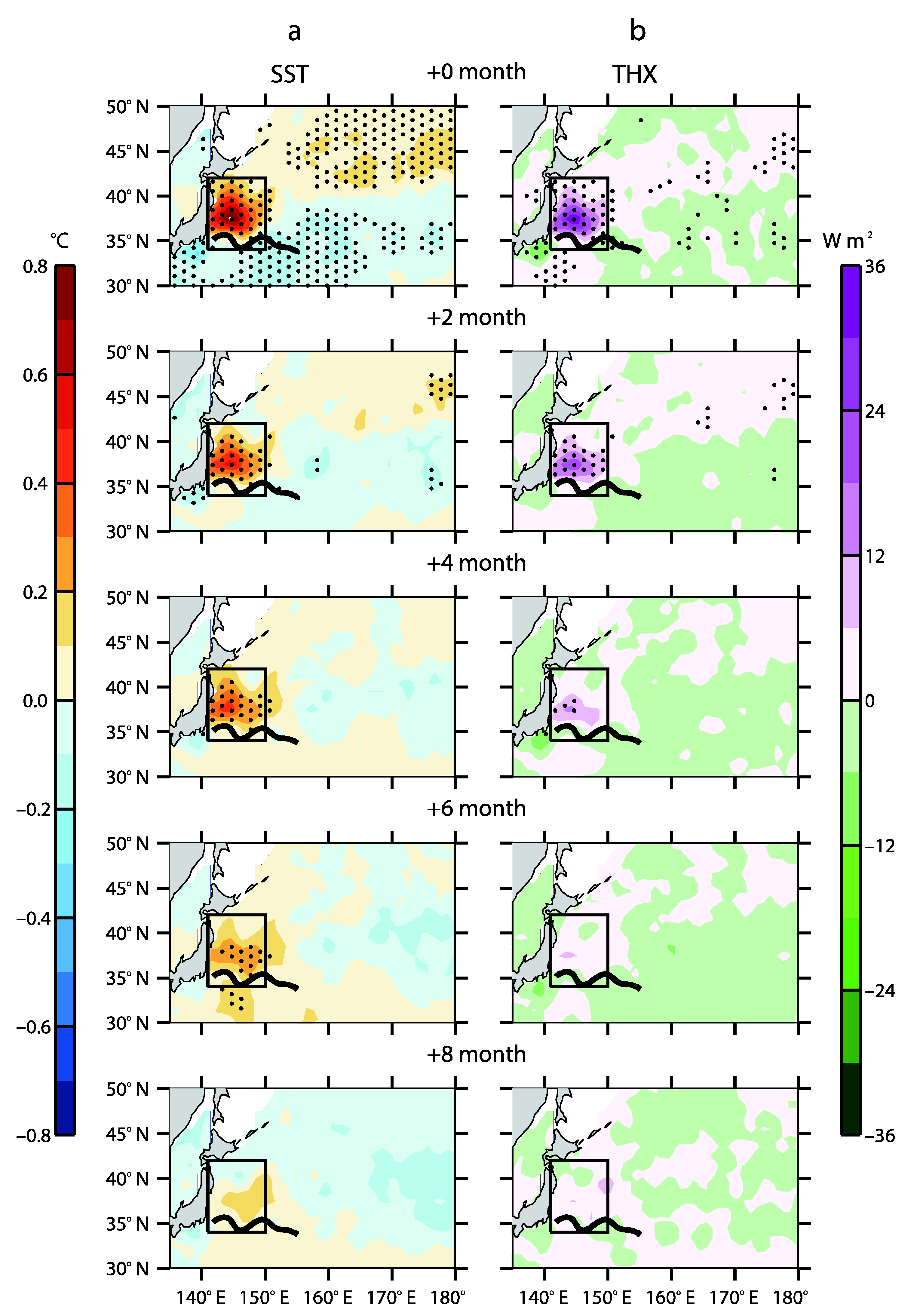
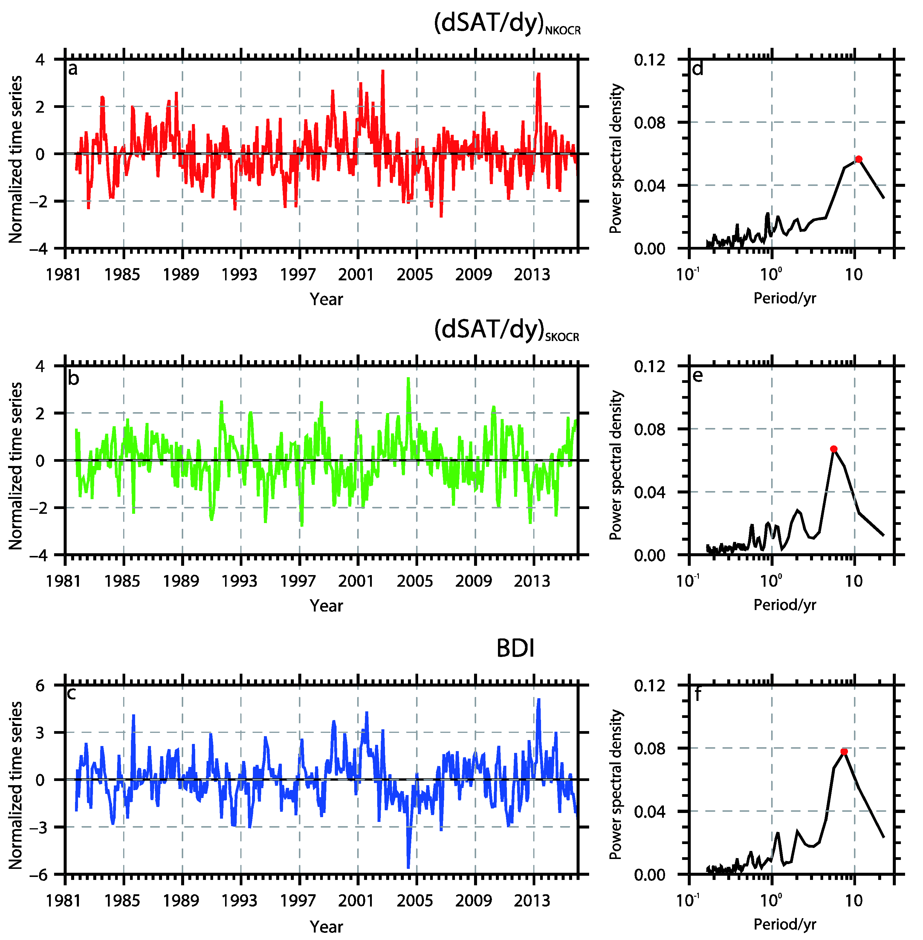
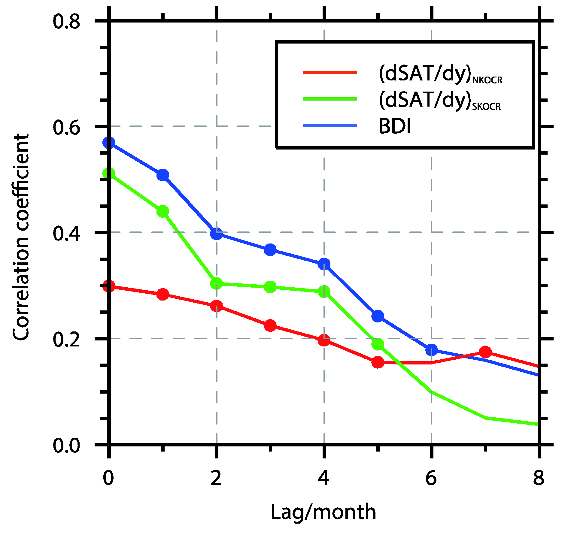
5. Impacts on the Air–Sea Heat Flux and Near-Surface Baroclinicity

Based on the EAI, the climatic effects of long-term KE eddy activity variation can also be studied. The impacts of these oceanic changes on the SST that generates the heat release at air–sea interface are important physical processes to understand how the KE eddy activity variation affects the climate, which are explored in the following. Figure 5 shows the linear regressions of the SST and surface turbulent heat flux (sensible + latent) onto the EAI when the SST and heat flux lag the EAI by 0–8 months. Note that the SST data utilized here are also derived from the OAflux product to keep consistency with heat-flux data. However, the results remain nearly the same with those derived from NOAA OISST. For the lag time of 0 months, in west of 155° E, significant positive and negative SST anomalies appear to the north and south of the KE jet around 35° N, respectively (Figure 5a). Among these anomalies, the SST warming over the KOCR is exceptionally strong. This reflects the SST fingerprints of strengthened KE eddy activity as analyzed in Section 3.1. In addition to these SST anomalies, there are significant negative SST anomalies over the downstream KE region in east of 155° E (Figure 5a). However, these SST anomalies are not supposed to be induced by KE eddy activity variation and can be regarded as the imprints of KE jet fluctuations associated with the EAI. Qiu [38] indicated that the anomalous heat advection by the weakened and southward-moving KE jet can cool the SST over the whole KE region. Because the KE eddy activity shows negative correlations with the KE jet strength and position (Table 1), it naturally shows the negative correlations with the SST anomalies over the downstream KE region. Moreover, significant positive SST anomalies are also present over the subpolar western North Pacific to the east of 155° E (Figure 5a). According to Révelard et al. [39], these SST anomalies may be explained as the response to the easterly-wind anomalies associated with the negative KE SSH index that is significantly correlated with the positive EAI (Table 1).
Meanwhile, the surface turbulent heat flux shows a similar distribution to the above SST pattern: significant positive (negative) heat-flux anomalies coincide with the regions where positive (negative) SST anomalies exist (Figure 5b). Here the positive heat flux denotes the heat that is transferred from the ocean into the atmosphere. This suggests a damping effect of heat flux on SST changes. From these heat-flux anomalies, it can be seen that significant heat loss from ocean mainly occurs over the KOCR (Figure 5b), consistent with the strong warm SST anomalies there. After 2–4 months, the SST and heat-flux anomalies in east of 155° E, which are not caused by the KE eddy activity variation, gradually disappear (Figure 5). In contrast, over the KOCR, the SST warming, and its accompanying positive heat-flux anomalies, are still pronounced (Figure 5). As indicated by Frankignoul et al. [40], these heat-flux anomalies with a lag of more than one month can be considered as the thermal forcing induced by the KE eddy activity variation on the atmosphere. In response to this anomalous heat supply from the ocean, significant surface-air-temperature (SAT) warming also emerges over the KOCR, which can persist over 4 months and become insignificant after that (Figure 6a). Similar results can also be obtained from ERA-Interim reanalysis (figure not shown). This SAT warming causes the increase and decrease in near-surface baroclinicity over the northern and southern parts of KOCR, respectively (Figure 6b). Here the baroclinicity is measured by the meridional SAT gradient (dSAT/dy) according to Sampe et al. [41], meaning that the large (small) meridional SAT gradient corresponds to a strong (weak) near-surface baroclinicity. As a result, a meridional dipole structure of anomalous near-surface baroclinicity over the KOCR is formed.
From the above analysis, it can be concluded that the strengthened KE eddy activity induces the pronounced heat release towards the atmosphere over the KOCR, which favors a significant SAT warming that can persist over 4 months, thus leading to the formation of a meridional dipole pattern of anomalous near-surface baroclinicity over this region. Although based on the KE SSH index, Masunaga et al. [42] has investigated the impacts of KE eddy activity variation on surface heat flux and baroclinicity over the KOCR; their results show that the KE eddy activity can only cause a single anomalous baroclinic zone over the southern part of KOCR rather than the meridional dipole structure identified here. This discrepancy reflects the differences between the EAI and the SSH index even though they are significantly correlated (Table 1). Furthermore, the persistent time of thermal forcing induced by the KE eddy activity variation was not analyzed in Masunaga et al. [42].
To further validate our finding, an index was developed to quantitatively depict the meridional dipole of anomalous near-surface baroclinicity (the baroclinicity dipole index: BDI); and is defined as follows:
BDI = ( dSAT / d y ) NKOCR ( dSAT / d y ) SKOCR ,
where (dSAT/dy)NKOCR and (dSAT/dy)SKOCR denote the normalized time series of equatorial SAT-gradient anomalies averaged over the northern (38°–42° N, 142°–150° E) and southern (34°–37° N, 141°–148° E) parts of KOCR, respectively (Figure 7a,b). The temporal evolution of BDI (Figure 7c) shows significant variation with a period of about 8 years (Figure 7f), which is identical to the long-term behavior in EAI (see Figure 2a). However, neither of (dSAT/dy)NKOCR or (dSAT/dy)SKOCR display the significant period of about 8 years (Figure 7d,e). Therefore, it is expected that the EAI is more closely related to the BDI than (dSAT/dy)NKOCR and (dSAT/dy)SKOCR. Indeed, as shown in Figure 8, the EAI shows significant simultaneous correlation with the BDI. This significant relationship can persist still until 6 months later and is obviously stronger than that between the EAI and (dSAT/dy)NKOCR or (dSAT/dy)SKOCR. This indicates that KE eddy activity variation exerts significant impacts not only on the (dSAT/dy)NKOCR but also on the (dSAT/dy)SKOCR, leading to an anomalous dipole pattern of near-surface baroclinicity over the KOCR, verifying the results shown in Figure 6b.
Many research works have pointed out that the near-surface baroclinicity is an important bridge that connects the midlatitude oceanic changes and the atmospheric circulation, e.g., [41,43,44,45,46,47,48]. For instance, the intensity and position changes of near-surface baroclinicity associated with the midlatitude SST anomalies can induce the consistent variations of tropospheric jet by modulating the atmospheric transient eddy activity. Motivated by these works, we also analyzed the relationship of EAI-related anomalous near-surface baroclinicity with the tropospheric jet to explore the possible impacts of long-term KE eddy activity variation on atmospheric circulation. As shown in Figure 9, the increase in (dSAT/dy)NKOCR corresponds to significant westerly anomalies around the jet stream over East Asia and on its northern flank (Figure 9a), favoring a strengthened and northward-moving East Asian jet. In contrast, the decrease in (dSAT/dy)SKOCR is related to the pronounced easterly winds that weaken the East Asian jet (Figure 9b). These opposite changes in (dSAT/dy)NKOCR and (dSAT/dy)SKOCR, which correspond to a positive BDI, are jointly associated with the significant easterly anomalies around the jet stream and westerly anomalies on its northern flank, leading to a weakened and northward-moving East Asian jet (Figure 9c).
According to these results, the KE eddy activity may have a close relationship with the East Asian jet through modulating the near-surface baroclinicity. Indeed, we found that the EAI is also related to significant easterly-wind anomalies that lead to a weakened East Asian jet but with a more northern position compared with those associated with the BDI (figure not shown). Because the East Asian jet is an important climate system that strongly modulates the rainfall and SAT over East Asia, e.g., [49,50,51,52], the KE eddy activity variation is likely to impact the East Asian climate through the bridge of tropospheric jet. Thus, the EAI may be a potentially useful indicator of East Asian climate variability. This question is vital to understand the climatic effects of long-term KE eddy activity variation, and must be addressed in future studies.

6. Concluding Remarks

In this paper, a new index was developed to detect the long-term variation in the KE eddy activity based on high-resolution satellite-derived SST data from September 1981 to December 2015. This new eddy activity index (EAI) was constructed based on the covariation between the KE EKE variation and SST anomalies over the KOCR, which gauges the strength of eddy-induced poleward heat transport. Compared with other existing KE indices, the EAI has the best performance in capturing the low-frequency KE eddy activity variability.
The analysis of EAI reveals that over the long term, changes in the KE eddy activity show a significant period of about 8 years and are not directly modulated by the wind-driven oceanic Rossby waves formed in the central North Pacific. Based on the EAI, we also found that the strengthened KE eddy activity can significantly enhance the ocean-to-atmosphere heat transfer over the KOCR and thus induce a pronounced SAT warming over this region. These SAT anomalies associated with the KE eddy activity variability further lead to an anomalous dipole pattern of near-surface baroclinicity that can persist for up to 6 months, favoring a weakened and northward-moving East Asian jet. The situation is opposite when the KE eddy activity is weakened.
Our analysis suggests the EAI is a potentially useful indicator of East Asian climate variability through the bridge of the tropospheric jet. Therefore, it is believed that the new eddy index, which provides more samples than the conventional EKE index, will facilitate future studies focusing on the climatic effects of the KE eddy activity variation.

Author Contributions

Conceptualization, P.Y. and C.Z.; methodology, X.C.; software, M.Y.; validation, P.Y., X.C. and Q.Z.; formal analysis, M.Y.; investigation, P.Y. and C.Z.; resources, P.Y.; data curation, Q.Z.; writing—original draft preparation, P.Y.; writing—review and editing, P.Y. and C.Z.; visualization, P.Y. and M.Y.; supervision, L.Z. and X.L.; project administration, X.L.; funding acquisition, L.Z. and X.L. All authors have read and agreed to the published version of the manuscript.

Funding

This research is supported by the National Natural Science Foundation of China (41975066, 41490642, and 41405051). P.Y. is supported by the Research Project of National University of Defense Technology (ZK20-45).

Acknowledgments

The authors sincerely acknowledge the three anonymous reviewers for their insightful comments, which greatly improved the quality of this manuscript.

Conflicts of Interest

The authors declare no conflict of interest.

References

  1. Stammer, D. On eddy characteristics, eddy transports, and mean flow properties. J. Phys. Oceanogr. 1998, 45, 1356–1375. [Google Scholar] [CrossRef]
  2. Gill, A.E.; Green, J.S.A.; Simmons, A.J. Energy partition in the large-scale ocean circulation and the production of mid-ocean eddies. J. Mar. Res. 1974, 21, 499–528. [Google Scholar] [CrossRef]
  3. Sasai, Y.; Richards, K.J.; Ishida, A.; Sasaki, H. Effects of cyclonic mesoscale eddies on the marine ecosystem in the Kuroshio Extension region using an eddy-resolving coupled physical-biological model. Ocean Dyn. 2010, 60, 693–704. [Google Scholar] [CrossRef]
  4. Chen, G.; Gan, J.; Xie, Q.; Chu, X.; Wang, D.; Hou, Y. Eddy heat and salt transports in the South China Sea and their seasonal modulations. J. Geophys. Res. 2012, 117, C05021. [Google Scholar] [CrossRef] [Green Version]
  5. Dong, C.; McWilliams, J.C.; Liu, Y.; Chen, D. Global heat and salt transports by eddy movement. Nat. Commun. 2014, 5, 3294. [Google Scholar] [CrossRef] [Green Version]
  6. Qiu, B.; Chen, S. Eddy-mean flow interaction in the decadally modulating Kuroshio Extension system. Deep Sea Res. Part II 2010, 57, 1098–1110. [Google Scholar] [CrossRef]
  7. Delman, A.S.; Mcclean, J.L.; Sprintall, J.; Talley, L.D.; Yulaeva, E.; Jayne, S.R. Effects of eddy vorticity forcing on the mean state of the kuroshio extension. J. Phys. Oceanogr. 2015, 45, 1356–1375. [Google Scholar] [CrossRef]
  8. Qiu, B.; Chen, S. Decadal variability in the formation of the North Pacific Subtropical Mode Water: Oceanic versus atmospheric control. J. Phys. Oceanogr. 2006, 36, 1365–1380. [Google Scholar] [CrossRef]
  9. Oka, E.; Qiu, B. Progress of North Pacific mode water research in the past decade. J. Oceanogr. 2012, 68, 5–20. [Google Scholar] [CrossRef]
  10. Putrasahan, D.A.; Miller, A.J.; Seo, H. Isolating mesoscale coupled ocean–atmosphere interactions in the kuroshio extension region. Dynam. Atmos. Oceans 2013, 63, 60–78. [Google Scholar] [CrossRef]
  11. Ma, J.; Xu, H.; Dong, C.; Lin, P.; Liu, Y. Atmospheric responses to oceanic eddies in the Kuroshio Extension region. J. Geophys. Res. Atmos. 2015, 120, 6313–6330. [Google Scholar] [CrossRef]
  12. Chen, L.; Liu, Q.; Jia, Y. Oceanic eddy-driven atmospheric secondary circulation in the winter Kuroshio Extension region. J. Oceanogr. 2016, 73, 295–307. [Google Scholar] [CrossRef]
  13. Sugimoto, S.; Aono, K.; Fukui, S. Local atmospheric response to warm mesoscale ocean eddies in the Kuroshio–Oyashio Confluence region. Sci. Rep. 2017, 7, 11871. [Google Scholar] [CrossRef] [PubMed] [Green Version]
  14. Ma, X.; Chang, P.; Saravanan, R.; Montuoro, R.; Hsieh, J.S.; Wu, D.; Lin, X.; Wu, L.; Jing, Z. Distant influence of Kuroshio eddies on North Pacific weather patterns? Sci. Rep. 2015, 5, 17785. [Google Scholar] [CrossRef] [Green Version]
  15. Ma, X.; Chang, P.; Saravanan, R.; Montuoro, R.; Nakamura, H.; Wu, D.; Lin, X.; Wu, L. Importance of resolving Kuroshio front and eddy influence in simulating the North Pacific storm track. J. Clim. 2017, 30, 1861–1880. [Google Scholar] [CrossRef]
  16. Zhang, C.; Liu, H.; Li, C.; Lin, P. Impacts of mesoscale sea surface temperature anomalies on the meridional shift of North Pacific storm track. Int. J. Climatol. 2019, 39, 5124–5139. [Google Scholar] [CrossRef] [Green Version]
  17. Qiu, B.; Chen, S. Variability of the Kuroshio Extension jet, recirculation gyre, and mesoscale eddies on decadal time scales. J. Phys. Oceanogr. 2005, 35, 2090–2103. [Google Scholar] [CrossRef]
  18. Itoh, S.; Yasuda, I. Characteristics of mesoscale eddies in the Kuroshio–Oyashio Extension region detected from the distribution of the sea surface height anomaly. J. Phys. Oceanogr. 2010, 40, 1018–1034. [Google Scholar] [CrossRef]
  19. Sugimoto, S.; Hanawa, K. Roles of SST anomalies on the wintertime turbulent heat fluxes in the Kuroshio–Oyashio Confluence Region: Influences of warm eddies detached from the Kuroshio Extension. J. Clim. 2011, 24, 6551–6561. [Google Scholar] [CrossRef]
  20. Reynolds, R.W.; Smith, T.M.; Liu, C.; Chelton, D.B.; Casey, K.S.; Schlax, M.G. Daily high-resolution-blended analyses for sea surface temperature. J. Clim. 2007, 20, 5473–5496. [Google Scholar] [CrossRef]
  21. Yu, L.; Jin, X.; Weller, R.A. Multidecade Global Flux Datasets from the Objectively Analyzed Air–Sea Fluxes (OAFlux) Project: Latent and Sensible Heat Fluxes, Ocean Evaporation, and Related Surface Meteorological Variables. Woods Hole Oceanographic Institution OAFlux Project Tech. Rep. 2008. Available online: http://oaflux.whoi.edu/pdfs/OAFlux_TechReport_3rd_release.pdf (accessed on 2 June 2020).
  22. Ducet, N.; Le Traon, P.Y.; Reverdin, G. Global high-resolution mapping of ocean circulation from TOPEX/Poseidon and ERS-1 and -2. J. Geophys. Res. 2000, 105, 19477–19498. [Google Scholar] [CrossRef]
  23. Carton, J.A.; Giese, B. A reanalysis of ocean climate using Simple Ocean Data Assimilation (SODA). Mon. Weather Rev. 2008, 136, 2999–3017. [Google Scholar] [CrossRef]
  24. Dee, D.P.; Uppala, S.M.; Simmons, A.J.; Berrisford, P.; Poli, P.; Kobayashi, S.; Andrae, U.; Balmaseda, M.A.; Balsamo, G.; Bauer, P.; et al. The ERA-Interim reanalysis: Configuration and performance of the data assimilation system. Q. J. R. Meteorol. Soc. 2011, 137, 553–597. [Google Scholar] [CrossRef]
  25. Ding, R.Q.; Li, J.P.; Tseng, Y.H. The impact of South Pacific extratropical forcing on ENSO and comparisons with the North Pacific. Clim. Dyn. 2015, 44, 2017–2034. [Google Scholar] [CrossRef]
  26. Seo, Y.; Sugimoto, S.; Hanawa, K. Long-term variations of the Kuroshio Extension path in winter: Meridional movement and path state change. J. Clim. 2014, 27, 5929–5940. [Google Scholar] [CrossRef]
  27. Qiu, B.; Chen, S.M.; Schneider, N.; Taguchi, B. A coupled decadal prediction of the dynamic state of the Kuroshio Extension system. J. Clim. 2014, 27, 1751–1764. [Google Scholar] [CrossRef] [Green Version]
  28. Qiu, B.; Schneider, N.; Chen, S. Coupled decadal variability in the North Pacific: An observationally constrained idealized model. J. Clim. 2007, 20, 3602–3620. [Google Scholar] [CrossRef] [Green Version]
  29. Yu, P.; Zhang, L.; Zhang, Y.; Deng, B. Interdecadal change of winter SST variability in the Kuroshio Extension region and its linkage with Aleutian atmospheric low pressure system. Acta Oceanol. Sin. 2016, 35, 24–37. [Google Scholar] [CrossRef]
  30. Nonaka, M.; Nakamura, H.; Tanimoto, Y.; Kagimoto, T.; Sasaki, H. Decadal variability in the Kuroshio–Oyashio Extension simulated in an eddy-resolving OGCM. J. Clim. 2006, 19, 1970–1989. [Google Scholar] [CrossRef] [Green Version]
  31. Ceballos, L.I.; Di Lorenzo, E.; Hoyos, C.D.; Schneider, N.; Taguchi, B. North Pacific Gyre Oscillation synchronizes climate fluctuations in the eastern and western boundary systems. J. Clim. 2009, 22, 5163–5174. [Google Scholar] [CrossRef] [Green Version]
  32. Sasaki, Y.N.; Schneider, N. Decadal shifts of the Kuroshio Extension jet: Application of thin-jet theory. J. Phys. Oceanogr. 2011, 41, 979–993. [Google Scholar] [CrossRef]
  33. Yang, Y.; Liang, X.; Qiu, B.; Chen, S. On the decadal variability of the eddy kinetic energy in the Kuroshio Extension. J. Phys. Oceanogr. 2017, 47, 1169–1187. [Google Scholar] [CrossRef]
  34. Sugimoto, S.; Hanawa, K. Relationship between the path of the Kuroshio in the south of Japan and the path of the Kuroshio Extension in the east. J. Oceanogr. 2012, 68, 219–225. [Google Scholar] [CrossRef]
  35. Fu, L.; Qiu, B. Low-frequency variability of the North Pacific Ocean: The roles of boundary-driven and wind-driven baroclinic Rossby waves. J. Geophys. Res. 2002, 107, 13–1–13–10. [Google Scholar] [CrossRef]
  36. Pierini, S. A Kuroshio Extension System model study: Decadal chaotic self-sustained oscillations. J. Phys. Oceanogr. 2006, 36, 1605–1625. [Google Scholar] [CrossRef]
  37. Pierini, S.; Dijkstra, H.A.; Riccio, A. A nonlinear theory of the Kuroshio Extension bimodality. J. Phys. Oceanogr. 2009, 39, 2212–2229. [Google Scholar] [CrossRef]
  38. Qiu, B. Interannual variability of the Kuroshio Extension and its impact on the wintertime SST field. J. Phys. Oceanogr. 2000, 30, 1486–1502. [Google Scholar] [CrossRef]
  39. Révelard, A.; Frankignoul, C.; Sennéchael, N.; Kwon, Y.O.; Qiu, B. Influence of the decadal variability of the Kuroshio Extension on the atmospheric circulation in the cold season. J. Clim. 2016, 29, 2123–2144. [Google Scholar] [CrossRef]
  40. Frankignoul, C.; Czaja, A.; L’Heveder, B. Air-sea feedback in the North Atlantic and surface boundary conditions for ocean models. J. Clim. 1998, 11, 2310–2324. [Google Scholar] [CrossRef] [Green Version]
  41. Sampe, T.; Nakamura, H.; Goto, A.; Ohfuchi, W. Significance of a midlatitude SST frontal zone in the formation of a storm track and an eddy-driven westerly jet. J. Clim. 2010, 23, 1793–6128. [Google Scholar] [CrossRef]
  42. Masunaga, R.; Nakamura, H.; Miyasaka, T.; Nishii, K.; Qiu, B. Interannual modulations of oceanic imprints on the wintertime atmospheric boundary layer under the changing dynamical regimes of the Kuroshio Extension. J. Clim. 2016, 29, 3273–3296. [Google Scholar] [CrossRef] [Green Version]
  43. Nakamura, H.; Sampe, T.; Goto, A.; Ohfuchi, W.; Xie, S.-P. On the importance of midlatitude oceanic frontal zones for the mean state and dominant variability in the tropospheric circulation. Geophys. Res. Lett. 2008, 35, L15709. [Google Scholar] [CrossRef] [Green Version]
  44. Nakamura, M.; Yamane, S. Dominant anomaly patterns in the near-surface baroclinicity and accompanying anomalies in the atmosphere and oceans. Part I: North Atlantic basin. J. Clim. 2009, 22, 880–904. [Google Scholar] [CrossRef]
  45. Nakamura, M.; Yamane, S. Dominant anomaly patterns in the near-surface baroclinicity and accompanying anomalies in the atmosphere and oceans. Part II: North Pacific basin. J. Clim. 2010, 23, 6445–6467. [Google Scholar] [CrossRef]
  46. Nakamura, M.; Miyama, T. Impacts of the Oyashio temperature front on the regional climate. J. Clim. 2014, 27, 7861–7873. [Google Scholar] [CrossRef]
  47. Fang, J.; Yang, X. Structure and dynamics of decadal anomalies in the wintertime midlatitude North Pacific ocean–atmosphere system. Clim. Dyn. 2016, 47, 1989–2007. [Google Scholar] [CrossRef] [Green Version]
  48. Chan, D.; Zhang, Y.; Wu, Q.; Dai, X. Quantifying the dynamics of the interannual variabilities of the wintertime East Asian Jet Core. Clim. Dyn. 2020, 54, 2447–2463. [Google Scholar] [CrossRef] [Green Version]
  49. Kuang, X.; Zhang, Y. Impact of the position abnormalities of East Asian subtropical westerly jet on summer precipitation in middle-lower reaches of Yangtze River. Plateau Meteorol. 2006, 25, 382–389. [Google Scholar]
  50. Yang, L.; Wu, B. Interdecadal variations of the East Asian winter surface air temperature and possible causes. Chin. Sci. Bull. 2013, 58, 3969–3977. [Google Scholar] [CrossRef] [Green Version]
  51. He, C.; Lin, A.; Gu, D.; Li, C.; Zheng, B.; Zhou, T. Interannual variability of Eastern China Summer Rainfall: The origins of the meridional triple and dipole modes. Clim. Dyn. 2017, 48, 683–696. [Google Scholar] [CrossRef] [Green Version]
  52. Yu, P.; Zhang, L.; Zhong, Q. Contrasting relationship between the Kuroshio Extension and the East Asian summer monsoon before and after the late 1980s. Clim. Dyn. 2019, 52, 929–950. [Google Scholar] [CrossRef]
Figure 1. (a) Climatological distribution of the eddy kinetic energy (EKE) over the North Pacific. The purple box indicates the domain of Figure 1b (30°–44° N, 136°–155° E). The black box denotes the Kuroshio Extension (KE) region (32°–38° N, 142°–155° E). (b) Correlations of the sea surface temperature (SST) anomalies onto the normalized EKE time series averaged over the KE region. The white contours indicate the regions exceeding the 95% confidence level. The purple box indicates the Kuroshio–Oyashio confluence region (KOCR) (34°–42° N, 141°–150° E). The thick black line represents the mean KE jet axis, which is defined as the 110-cm SSH contour. The three black boxes denote the regions used to define the new eddy activity index (EAI) (see text for details). (c) Time series of the EAI (blue line) and the EKE (red line) of KE.
Atmosphere 11 00792 g001
Figure 2. Power spectra of the normalized (a) EAI, (b) EKE, (c) jet strength, (d) jet pathlength, (e) jet position, and (f) SSH indices of KE. Red (blue) dots indicate the spectral peak significant (insignificant) at the 95% confidence level.
Atmosphere 11 00792 g002
Figure 3. (a) Hovmöller plot of the 37-month running mean SSH anomalies averaged over the 33°–35° N band. These SSH anomaly data were merged from the AVISO satellite data for 1993–2015 and the SODA reanalysis data for 1981–1992. (b) Lag–longitude correlation diagram of the 37-month running mean EAI with the SSH anomalies in (a). Positive lags mean that the EAI leads the SSH anomalies. The stippled areas indicate statistical significance above the 95% confidence level.
Atmosphere 11 00792 g003
Figure 4. Same as in Figure 3, but for (a) the 37-month running mean SSH anomalies averaged over the 33°–35° N band from the outputs of the wind-driven Rossby wave model and for (b) their lead–lag correlations with the EAI.
Atmosphere 11 00792 g004
Figure 5. Regressions of the (a) SST and (b) turbulent heat-flux anomalies onto the normalized EAI when the SST and heat flux lag the EAI by 0–8 months. The black box indicates the KOCR. The thick black line represents the mean KE jet axis. The stippled areas indicate statistical significance above the 90% confidence level.
Atmosphere 11 00792 g005
Figure 6. Same as in Figure 5, but for the (a) SAT and (b) its meridional-gradient (dSAT/dy) anomalies. The black box and the thick black line in (a) denote the KOCR and mean KE jet axis, respectively. The black boxes in (b) indicate the regions used to define the BDI (see text for details).
Atmosphere 11 00792 g006
Figure 7. Normalized time series of the (a) (dSAT/dy)NKOCR, (b) (dSAT/dy)SKOCR, and (c) BDI and their corresponding power spectra (df). Red dots indicate the spectral peak significant at the 95% confidence level.
Atmosphere 11 00792 g007
Figure 8. Correlation coefficients of the EAI with the (dSAT/dy)NKOCR (red line), (dSAT/dy)SKOCR (green line), and BDI (blue line) after a lag of 0–8 months. Note that the sign of (dSAT/dy)SKOCR is reversed here for convenience of comparison. Dots indicate the correlations significant at the 95% confidence level.
Atmosphere 11 00792 g008
Figure 9. Regressions of the 500-hPa zonal-wind anomalies onto the normalized (a) (dSAT/dy)NKOCR, (b) (dSAT/dy)SKOCR, and (c) BDI. Note that the sign of (dSAT/dy)SKOCR is reversed here for convenience of comparison. The thick grey contours indicate the climatological East Asian jet (20 m s−1 contour). The stippled areas indicate statistical significance above the 90% confidence level.
Atmosphere 11 00792 g009
Table 1. Correlation coefficients between the EKE, EAI, and other existing KE indices: jet strength, pathlength, position, and SSH index with the monthly/annual resolution.
EAIJet StrengthJet PathlengthJet PositionSSH
EKE0.57 */0.83 *–0.31 */–0.63 *0.32 */0.60 *–0.01/–0.27–0.38 */–0.54 *
EAI-–0.53 */–0.63 *0.40 */0.68 *–0.20/–0.41 *–0.42 */–0.60 *
* Correlation significant at the 95% confidence level.

