Mathematical Modeling of Vortex Interaction Using a Three-Layer Quasigeostrophic Model. Part 1: Point-Vortex Approach

Abstract

The theory of point vortices is used to explain the interaction of a surface vortex with subsurface vortices in the framework of a three-layer quasigeostrophic model. Theory and numerical experiments are used to calculate the interaction between one surface and one subsurface vortex. Then, the configuration with one surface vortex and two subsurface vortices of equal and opposite vorticities (a subsurface vortex dipole) is considered. Numerical experiments show that the self-propelling dipole can either be captured by the surface vortex, move in its vicinity, or finally be completely ejected on an unbounded trajectory. Asymmetric dipoles make loop-like motions and remain in the vicinity of the surface vortex. This model can help interpret the motions of Lagrangian floats at various depths in the ocean.

1. Introduction

The theory of point vortices (vertical vortex lines of finite length) in a flat liquid layer, going back to the pioneering works of Helmholtz, Kirchhoff, Gröbli, and Thomson (Lord Kelvin) [1,2,3,4,5], arose to a large extent from the need to explain the properties of vortex movements in the atmosphere and ocean. Further development of the theory of point vortices is reflected in monographs and reviews [6,7,8,9,10,11,12,13,14,15,16]. The classical concept of point vortices was used in problems of meteorology [17,18,19,20,21,22,23] and oceanography in [24,25,26,27,28,29,30]. Gryanik first generalized the theory of two-dimensional vortices to the case of a two-layer [31] and then to an N-layer rotating fluid [32]. These works found their application in numerous problems of geophysical content [33,34,35,36,37,38,39,40,41,42,43,44,45,46,47,48,49,50,51,52,53,54,55,56,57,58,59,60,61,62,63].

In this paper, we use a quasigeostrophic model to study the features of the interaction between one vortex of the upper layer and one/two vortices of the middle layer of a three-layer rotating fluid. The vortex of the upper layer is a prototype of a surface ocean vortex (many such vortices occupy the upper 500–600 m of 4000 m deep oceans). The vortices of the middle layer represent intrathermocline lens vortices, observed in all oceans, but especially common in the Northeastern Atlantic at depths of 600–1600 m [64,65]. Note that for the first time the idea of modeling intrathermocline lenses with point vortices of the intermediate layer was proposed by Hogg and Stommel in [37]. The lower layer will contain no vortex and will correspond to the deep ocean.

In [66,67], the SEMANE and MEDTOP cruise data were analyzed to study the interactions of intrathermocline vortices with a cyclonic surface vortex; however, due to intermittent data collection at sea, only a few snapshots of these interactions were obtained. This circumstance is the motivation for the present work. In this first part, we restrict ourselves to the motion of point vortices. In the second part of the article, the dynamics of vortex patches will be considered.

After presenting the model equations and the numerical method (Section 2), in Section 3 we will study the different cases of interaction of a surface vortex with the deeper vortex/vortices. Finally, in Section 4, a discussion and conclusion are provided.

2. Three-Layer Model

We use a three-layer quasigeostrophic model with the following parameters characteristic of the North Atlantic Ocean Basin and water stratification: the total depth is 4 km, and the thicknesses of the upper, middle, and lower layers are H₁ = 600 m, H₂ = 1000 m, and H₃ = 2400 m, respectively. So, dimensionless thicknesses of these layers are 0.15, 0.25, and 0.6, respectively. The first and second deformation radii calculated from the average density stratification correspond to the horizontal scale where the Coriolis and buoyancy effects are similar in magnitude. These deformation radii are as follows: Rd₁ = 32 km and Rd₂ = 15 km [67].

A dynamical system modeling the evolution of an arbitrary number of vortices with intensities ${\kappa }_m^n,$ where $m=1, 2, 3$ is the layer number and $n=1, 2, \dots , N_n$ is the number of vortices in the nth layer, has the Hamiltonian [36,42]

$$\mathscr{H}=-\frac{1}{4\pi }{\displaystyle \sum }_{i=1}^3{\displaystyle \sum }_{m=1}^3{\displaystyle \sum }_{\begin{array}{c}l,n=1\\ n\ne l if m=i\end{array}}^{N_l, N_n}{\displaystyle \sum }_{j=2}^3{q}_{ij}{s}_{jm}{\kappa }_m^n{\kappa }_i^l\left(\ln \left(r_{mi}^{nl}\right)+ {\mathrm{K}}_0\left({\gamma }_{j-1}{r}_{mi}^{nl}\right)\right)$$

(1)

with canonical variables $g_m^n=x_m^n$ and $p_m^n={\kappa }_m^n{y}_m^n/2.$ Here, ${\mathrm{K}}_0$ is a modified Bessel function of zero order; ${\gamma }_1,{\gamma }_2$ are the parameters inversely proportional to the first and second deformation radii, respectively; $r_{mi}^{nl}=\sqrt{{\left(x_m^n-x_i^l\right)}^2+{\left(y_m^n-y_i^l\right)}^2}$ is the distance between vortices with intensities ${\kappa }_m^n$ and ${\kappa }_i^l$, $q_{ij};$ and и $s_{ij}$ are auxiliary $3\times 3$ matrix elements: their form is given in the second part of the article.

The Hamiltonian form of the equations of motion is

$${\dot{g}}_m^n=\frac{\partial \mathscr{H}}{\partial p_m^n}\equiv J\left(g_m^n, \mathscr{H}\right), {\dot{p}}_m^n=-\frac{\partial \mathscr{H}}{\partial g_m^n}\equiv J\left(p_m^n, \mathscr{H}\right), m=1, 2, 3; n=1, 2, \dots , N_n$$

(2)

In addition to the Hamiltonian (1), the system has integral invariants:

$$\left[P_x; P_y;M\right]={\displaystyle \sum }_{m=1}^3{\displaystyle \sum }_{n=1}^{N_m}{h}_m{\kappa }_m^n\left[x_m^n; y_m^n; \left({\left(x_m^n\right)}^2+{\left(y_m^n\right)}^2\right)\right],$$

(3)

i.e., the linear impulses $P_x,P_y$ and the angular momentum $M.$

In Cartesian coordinates, the equations of motion of the vortices have the form

$${\dot{x}}_i^l=-\frac{1}{2\pi }\left[{\displaystyle \sum }_{m=1}^3{\displaystyle \sum }_{\begin{array}{c}n=1\\ n\ne l if m=i\end{array}}^{N_n}{\displaystyle \sum }_{j=2}^3{q}_{ij}{s}_{jm}{\kappa }_m^n\frac{y_i^l-y_m^n}{{\left(r_{im}^{ln}\right)}^2}\left({\gamma }_1{r}_{im}^{ln} {\mathrm{K}}_1\left({\gamma }_1{r}_{im}^{ln}\right)-1\right) \right]$$

(4)

$${\dot{y}}_i^l=\frac{1}{2\pi }\left[{\displaystyle \sum }_{m=1}^3{\displaystyle \sum }_{\begin{array}{c}n=1\\ n\ne l if m=i\end{array}}^{N_n}{\displaystyle \sum }_{j=2}^3{q}_{ij}{s}_{jm}{\kappa }_m^n\frac{x_i^l-x_m^n}{{\left(r_{im}^{ln}\right)}^2}\left({\gamma }_1{r}_{im}^{ln} {\mathrm{K}}_1\left({\gamma }_1{r}_{im}^{ln}\right)-1\right) \right]$$

(5)

3. Numerical Modeling of Vortex Interaction

In all numerical experiments, which solve Equations (2) and (3), we will assume that one cyclonic vortex is located in the upper layer ($N_1=1,{\kappa }_1^1$ > 0) and either one anticyclonic lens can be located in the middle layer $(N_2=1, {\kappa }_2^1<0),$ or two vortices of opposite signs $\left(N_2=2,{\kappa }_2^1<0,{\kappa }_2^2>0\right)$. We also introduce the notation for the effective intensity of a point vortex ${\Lambda }_i^j=h_i{\kappa }_i^j.$

3.1. Cyclonic Surfer Vortex and Anticyclonic Intrathermocline Lenses

Let us consider now ${\Lambda }_1^1=-{\Lambda }_2^1$; this is an analogue of a heton (a two-layer dipolar structure) [33].

We assume that the upper and middle layer vortices lie initially on the x axis and are separated by a distance L. We obtain from (3)

$${\dot{y}}_1^1={\dot{y}}_2^1\equiv V=\frac{{\Lambda }_1}{2\pi L}\left[\frac{q_{12}{s}_{22}}{s_{11}}\left({\gamma }_{1}L{\mathrm{K}}_1\left({\gamma }_{1}L\right)-1\right)-\frac{q_{13}{s}_{32}}{s_{12}}\left({\gamma }_{2}L{\mathrm{K}}_1\left({\gamma }_{2}L\right)-1\right)\right]$$

(6)

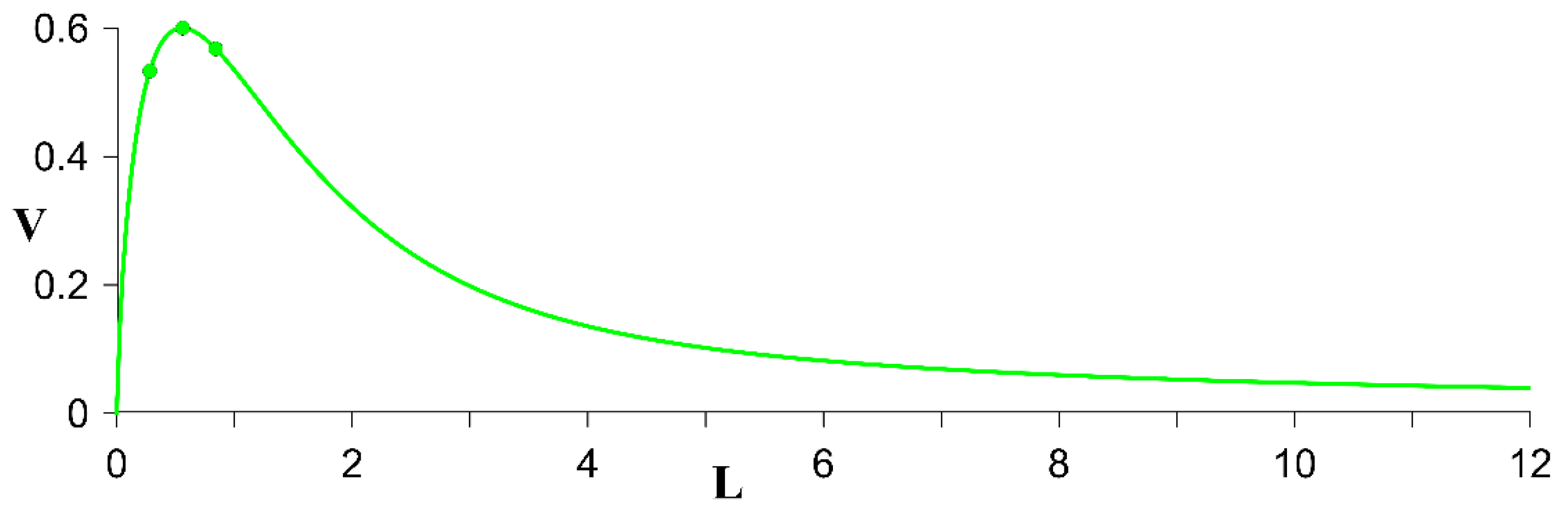
i.e., (1) at $L=0$, the structure will remain in place; (2) at $L>0$, the translational velocity of this two-layer vortex is a non-monotonic function of L, and its maximum is achieved at $L\approx 1.75·R{d}_1$ (green line in Figure 1).

If ${\Lambda }_1^1\ne -{\Lambda }_2^1$, then the vortices always rotate with angular velocity

$$\omega =\frac{1}{2\pi L^2}\left[\frac{q_{12}{s}_{22}}{s_{11}}{\Lambda }_1^1\left({\gamma }_{1}L{\mathrm{K}}_1\left({\gamma }_{1}L\right)-1\right)+\frac{q_{13}{s}_{32}}{s_{12}}{\Lambda }_2^1\left({\gamma }_{2}L{\mathrm{K}}_1\left({\gamma }_{2}L\right)-1\right)\right]$$

(7)

relative to the center of vorticity with coordinates

$$\left(x_c,y_c\right)=\frac{{\Lambda }_1^1\left(x_1^1,y_1^1\right)+{\Lambda }_2^1\left(x_2^1,y_2^1\right)}{{\Lambda }_1^1+{\Lambda }_2^1}$$

(8)

Figure 1 demonstrates the numerically obtained function V(L) for pointwise vortices in both the upper and middle layers (4) of the three-layer model.

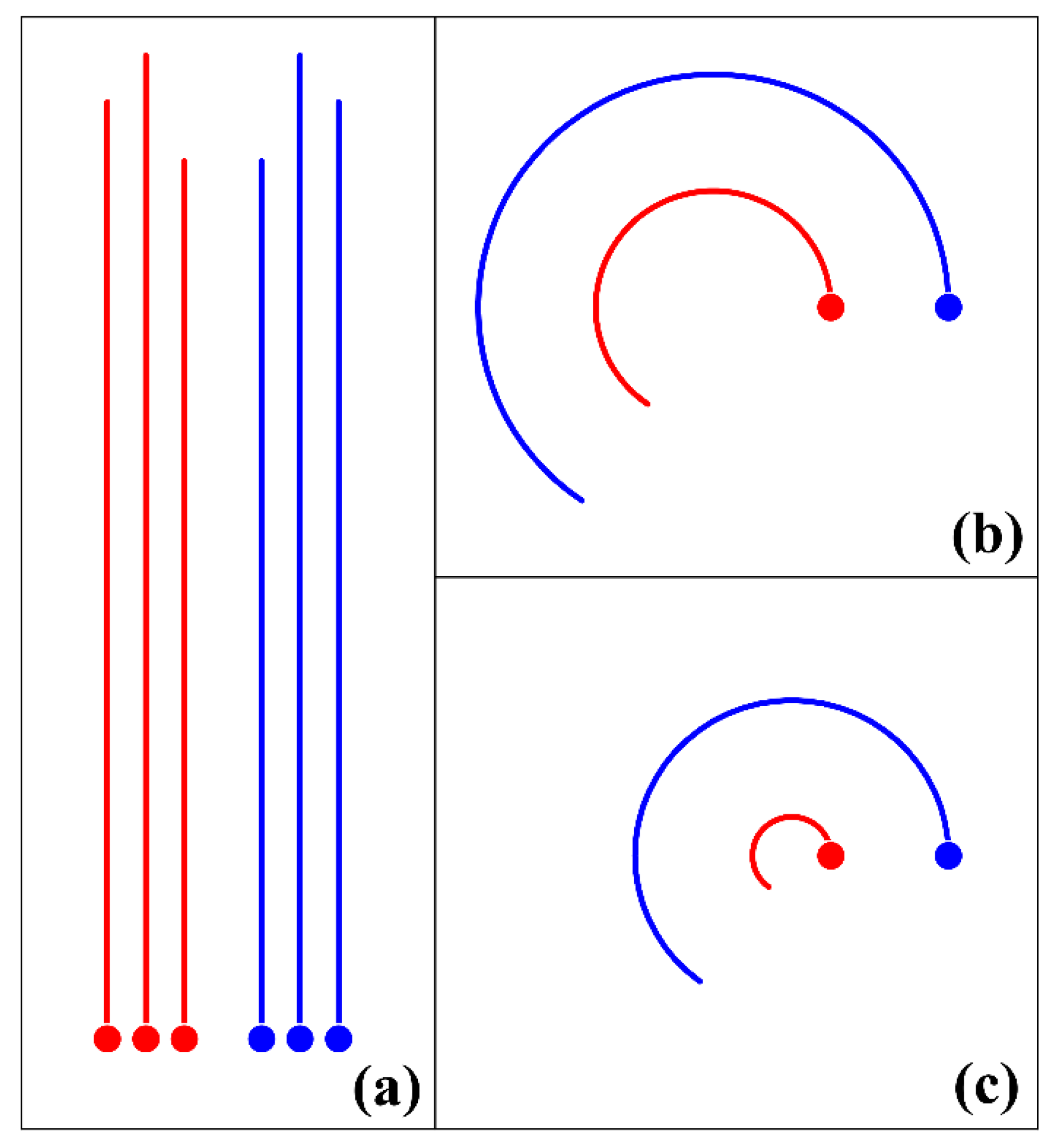
Markers on the green line in Figure 1 correspond to the values $L=0.56$ (where the maximum translational velocity of a point dipole takes place) and $L=0.28$ and $L=0.84$ (which are equidistant points from the maximum). For these values of $L$, the trajectories are presented in Figure 2a.

Figure 2a shows the initial sections of the vortex trajectories of two-layer dipoles calculated by Formulas (2) and (3) on the same time interval. Obviously, the end points of the straight segments repeat the profile of the green line in Figure 1. Note, that the non-monotonic character of $V\left(L\right)$ expresses the fundamental difference between baroclinic and barotropic dipoles, which have a singularity in velocity at $L=0$. Panels (b,c) show the initial trajectories of vortices at the same initial location but with a stronger cyclonic vortex in the upper layer. When the ratio ${\Lambda }_2^1/{\Lambda }_1^1$ is changed, the position of the center of vorticity changes, according to (6).

3.2. Interaction of a Surface Vortex with Two Middle Layer Vortices

3.2.1. Collinear Initial Configuration

Let us consider the simplest case when three vortices (one in the upper layer and two in the middle layer) initially form a symmetric collinear structure. The cyclonic vortex with effective intensity ${\Lambda }_1^1>0$ is still located in the upper layer; in the middle layer there are two vortices of opposite signs on opposite sides of the surface vortex, with ${\Lambda }_2^1=-{\Lambda }_2^2>0$. In such a situation two main interactions can govern the motion of the vortices of the middle layer: (a) an intralayer interaction, leading to uniform and rectilinear motion; (b) an interlayer interaction, leading to counterclockwise rotation under the influence of the surface cyclone. Obviously, the upper layer vortex does not undergo intralayer interaction; the pair of middle layer vortices advects it in the direction of its self-propagation. All these mechanisms act simultaneously and contribute to the observed motion of the vortex structure.

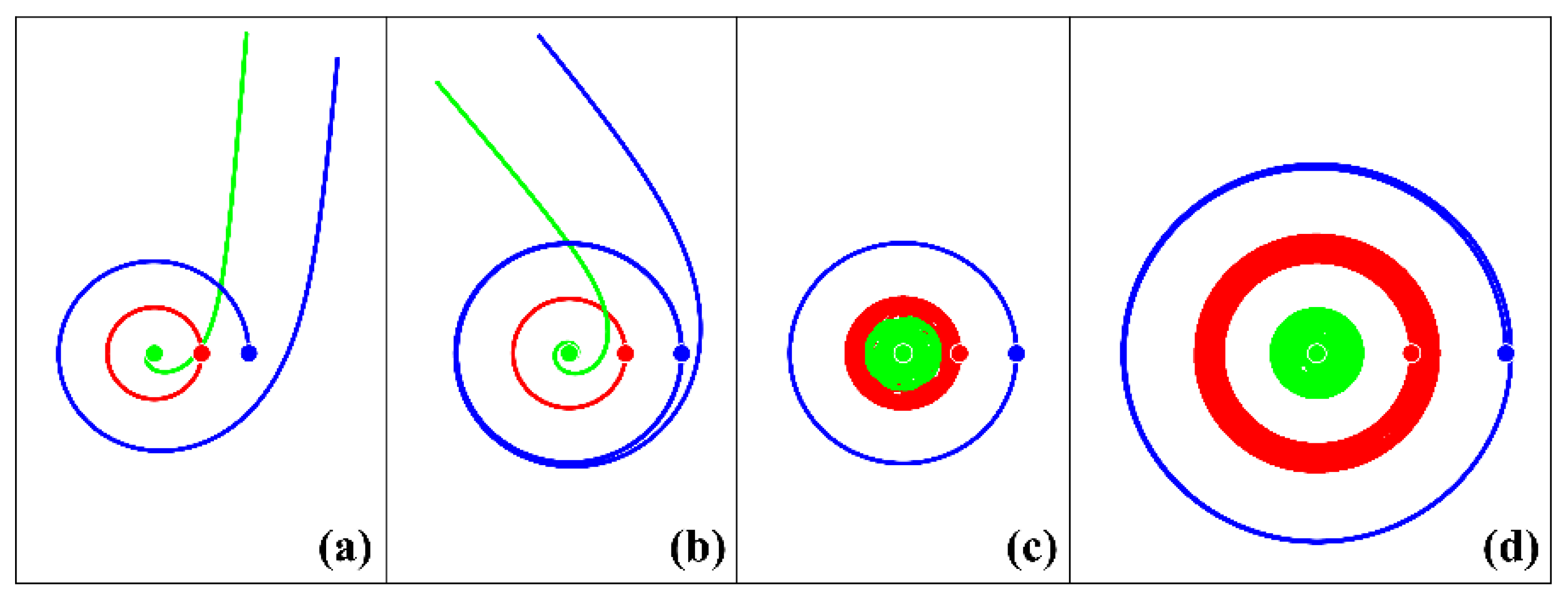
Figure 3 shows examples of trajectories of such a three-vortex structure. Here, as before, $L$ is the horizontal distance between the upper layer vortex and one of the middle layer vortices. Thus, the initial distance between the vortices of the middle layer is $2L$. The figure shows a change in regimes as the distance $L$ is increased, from a predominant intralayer interaction to a dominance of interlayer interaction.

In panel (a), for $L=1.00$, the middle layer vortices perform an incomplete counterclockwise rotation under the action of the surface cyclone, and then they pair up and leave the central region. The upper layer vortex performs an incomplete rotation with the middle layer vortices and stops. In panel (b), for $L=1.19$, the interlayer interaction is much stronger: all three vortices make seven incomplete rotations before the middle layer vortex pair leaves the central domain. In panel (c), where $L=1.20$, a spatially finite evolution takes place: all vortices follow a quasiperiodic counterclockwise trajectory inside a compact region. In the middle layer, the cyclonic vortex trajectory fills the central domain; the trajectories of the surface cyclone and the middle layer anticyclone are annular regions—intermediate and external, respectively. During this simulation, each vortex made about 778 rotations in the cyclonic direction. Thus, we can conclude that the boundary between the unbounded and bounded regimes lies in the interval $L\in \left[1.19;1.20\right].$ Finally, with $L=2$ (panel (d)), in the same time period, the number of rotations of each vortex is about 280.

3.2.2. Impact of the Two External Intrathermocline Vortices on the Surface Cyclone

Now, let two intrathermocline vortices of opposite signs be initially located relatively far from the surface vortex (in all the examples considered below, $y_2^1=y_2^2\equiv B=-16$ and $x_2^2=-x_2^1=L$ are assumed) and move towards it.

First, we consider the case of intrathermocline dipole, a particular case where the middle layer vortices form a dipolar structure, i.e., ${\Lambda }_2^1/{\Lambda }_2^2=-1$. Let us start with the simplest case when the vortices of the middle layer form a pair, symmetric with respect to the y axis; we consider different distances ($2L$) between the vortices in the pair.

In this case, for any value of $L$, the middle layer vortex motion deviates to the right of a straight trajectory due to the action of the upper layer cyclone. The cyclone itself, initially stationary, begins to move counterclockwise locally due to the action of the middle layer vortex pair. Numerical simulations show that for $L\le 0.6$, the dipole rotates around the surface cyclone and escapes to the left, while the cyclone slows down and stops over time without having performed a complete revolution. For $L\ge 0.7$, the surface vortex always traps the middle layer dipole, and the entire vortex structure rotates counterclockwise near the center of the domain for a finite duration. The middle layer cyclone trajectory lies inside the trajectory of the surface cyclone, and the anticyclonic lens rotates along an outer orbit. After this duration, the middle layer dipole moves away, and the surface cyclone stops.

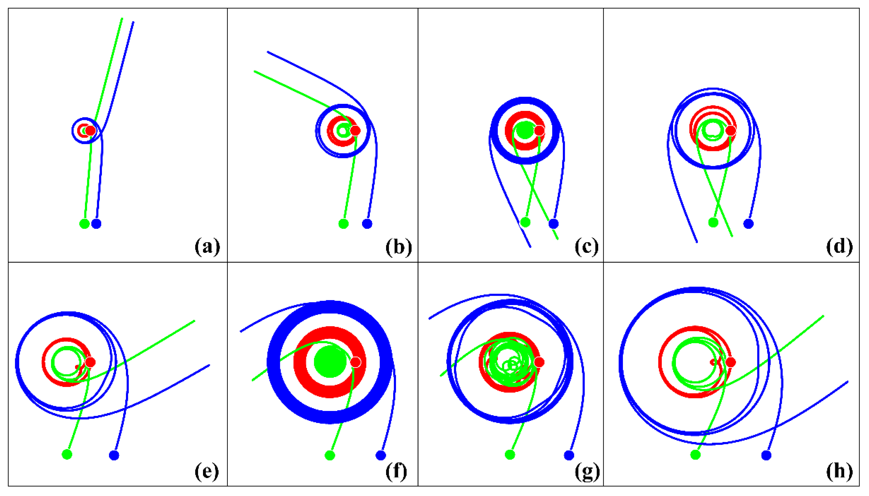
Figure 4 shows a gallery of the vortex trajectories at different time intervals (in the different panels) until the dipole structure leaves the central region (which is defined by $R\le 20$ around the origin). During the stage of bounded motion, the global vortex structure is composed of a two-layer cyclone with a “tilted axis” and a peripheral anticyclonic lens, all performing a counterclockwise rotation.

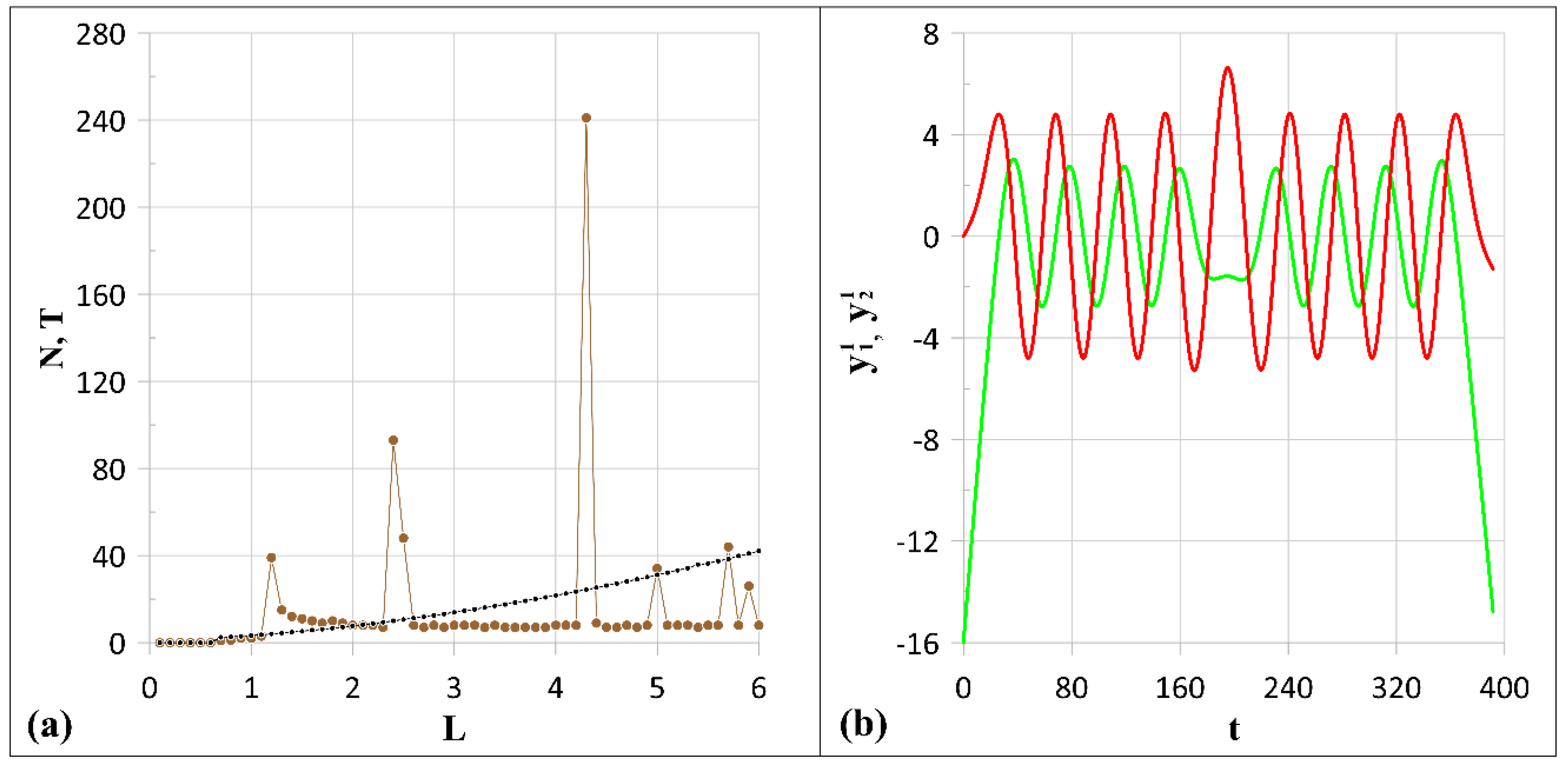
Figure 5a shows that the period of rotation $T$ of the vortex structure inside the bounded region monotonically increases with $L$, while the number of full revolutions $N$ is an irregular function of $L$. Note that this effect, known as “chattering” [9], is observed in other problems of vortex dynamics (for example, [68]). Two examples with surprisingly large values of $N$ are shown in panels (c) and (f) of Figure 4.

The transition between bounded and unbounded trajectories occurs when two velocity contributions become similar in magnitude: the first is the vortex velocity due to intralayer interaction, proportional to the singular function $1/L$, and the second is the velocity of vortices due to interlayer interaction, proportional to the regular non-monotonic function $\left(1/L-{\mathrm{K}}_1\left(L\right)\right)$. During the evolution of the vortex structure, the ratio between these contributions constantly changes; the prevalence of the first one leads to a transition towards unbounded trajectories, whereas the prevalence of the second one leads to bounded trajectories. The behavior of the vortices during such evolutions is illustrated in Figure 4b, which shows the time changes in the y-coordinates of the cyclones of the middle and upper layers at $L=4.8$, when $N=8$: initially the unbounded motion becomes bounded when $y_2^1$ decreases below $y_1^1$; then the amplitude of $y_1^1$ in the first half of the finite cycle initially increases to a maximum value, and $y_2^1$ decreases to a minimum; in the second half of the cycle, the changes in these functions are reversed; finally, $y_2^1$ reaches a limit value at which the subsurface vortex breaks out of the closed region, and the motion becomes unbounded again.

For large values of $N$ (for example, when $L=4.3$ and $N=241$, Figure 4f), there are several such subcycles, but at the end of each of them (except of the last one), the amplitude of $y_2^1$ has not yet reached its limit value.

Another interesting property in the case of large $N$ is that before reaching the unbounded regime, the annular regions filled by the trajectories of the surface cyclone and middle layer anticyclone expand significantly (as shown by the red and blue rings in Figure 4c,f).

Thus, when an intrathermocline pair runs into a surface cyclone, starting from a certain value of $L$ (here, at $B=-16,$ this value is $L\approx 1.7$) a temporary trapping occurs, followed by an expulsion of the dipole. Note that stationary localized regimes, observed for initially collinear vortices, as in Figure 3c,d, do not occur when a middle layer dipole runs into a surface cyclone.

Next, we consider the case of asymmetric middle layer vortices. Up to now, it has been assumed everywhere that the two middle layer vortices have the same effective intensity. However, observations [66,67] show that cyclones at intermediate depths are generally weaker than anticyclones. Such an asymmetry in the distribution of potential vorticity is now studied: we assume that ${\Lambda }_2^1/{\Lambda }_2^2=-1/2$.

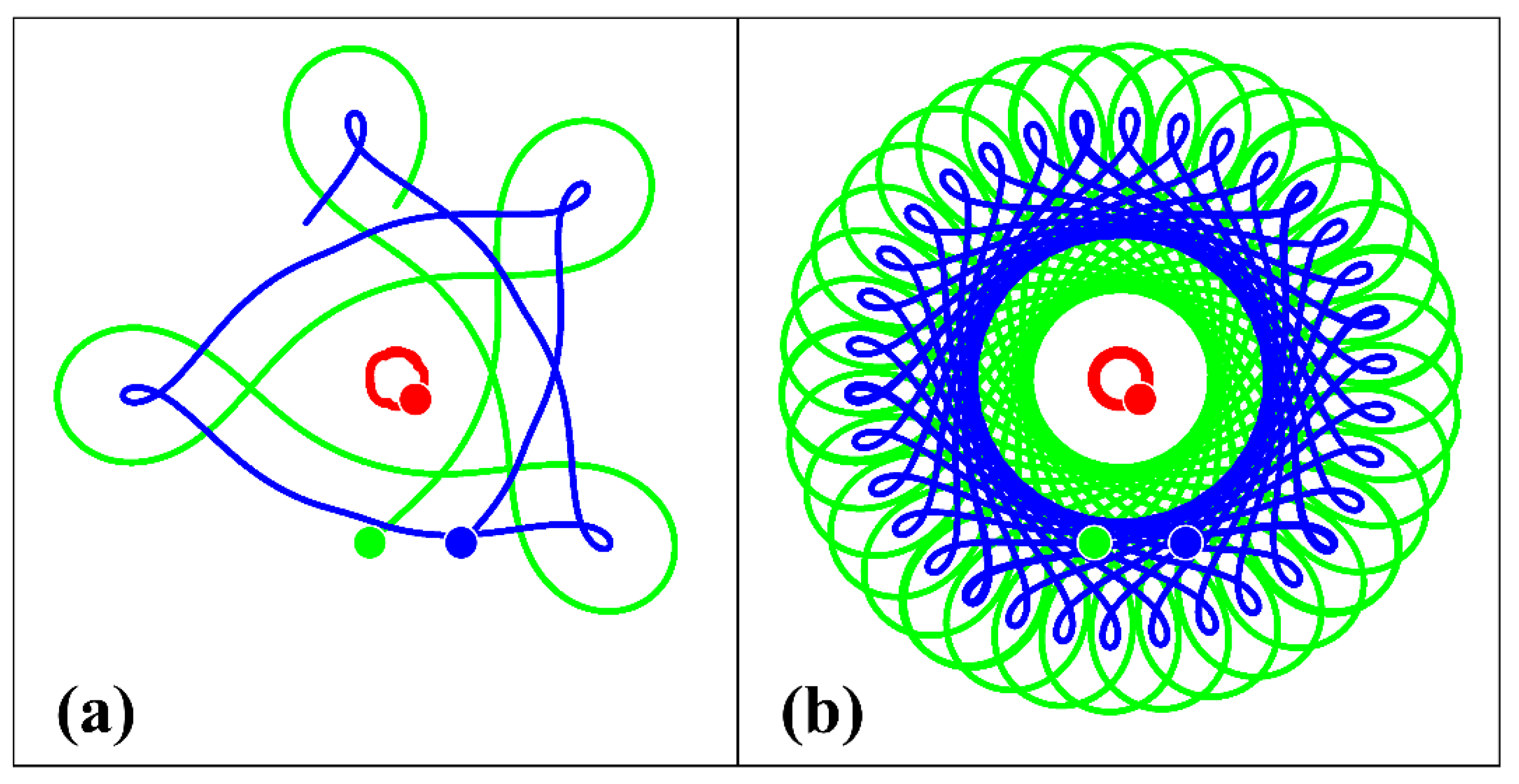
The interaction with the surface cyclone changes dramatically since the weak subsurface cyclone now rotates around the stronger anticyclone in the middle layer. In the general case, this weak subsurface cyclone follows a cycloidal trajectory both around the surface cyclone and around its anticyclonic partner. An example of this is shown in Figure 6. The trajectory of the middle layer cyclone (in green) is much wider than that of the anticyclonic vortex (in blue).

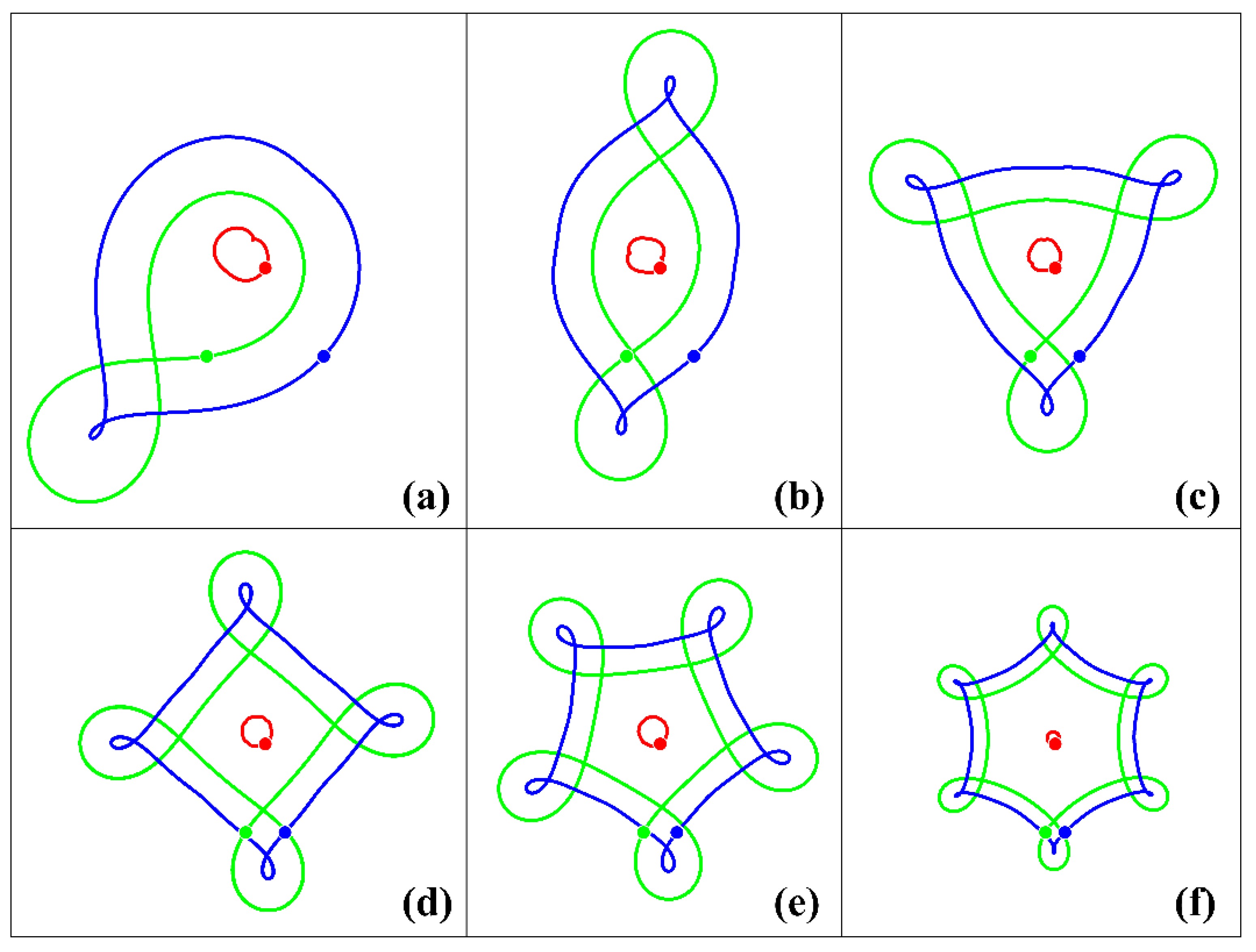
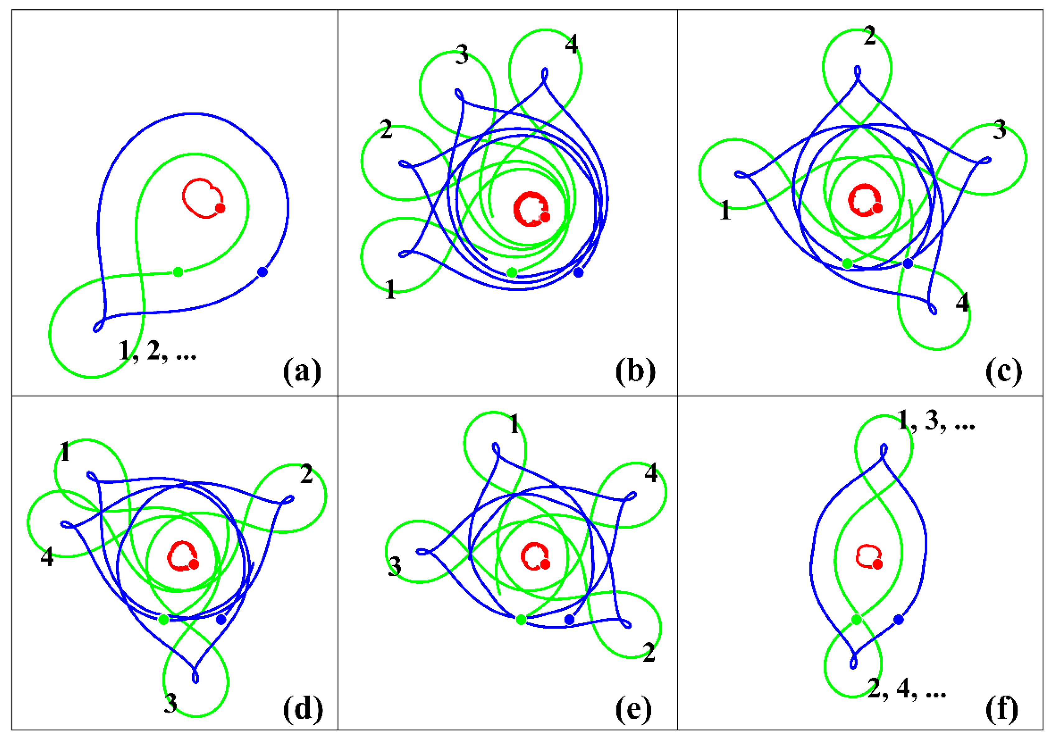
Depending on the value of parameter $L$, there is a countable number of periodic motions of the three vortices along closed trajectories, called “absolute choreographies” [69]. Examples of the first six choreographies are presented in Figure 7.

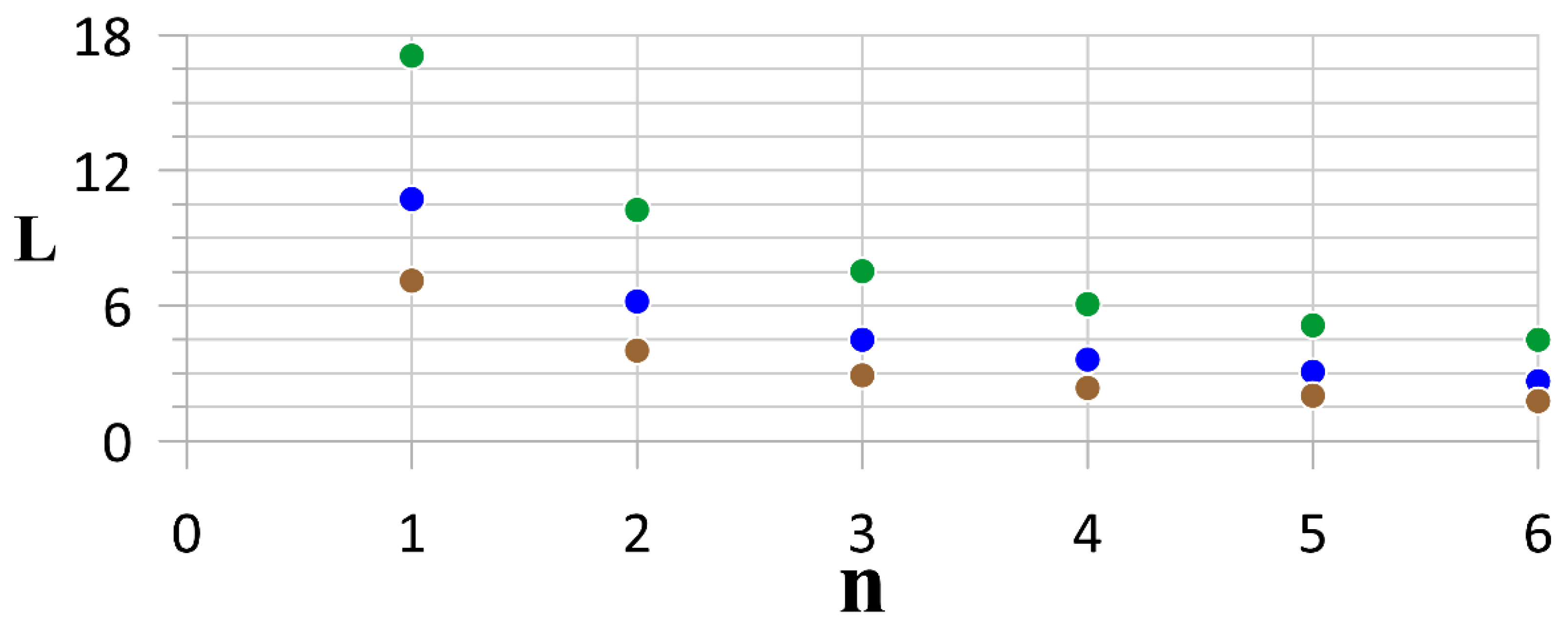
Thus, we have a discrete set of values $L_n$, decreasing with $n$, which corresponds to a family of $n$-fold symmetric configurations. Figure 8 shows $L\left(n\right)=L_n$ for various values of ${\Lambda }_2^1/{\Lambda }_1^1$.

Figure 8 shows that values $L_n$ decrease with increasing $n$ and with decreasing of intensity of subsurface vortices.

Finally, Figure 9 shows how the transition between one-mode to two-mode choreography occurs when the distance $L$ changes with a constant step $\Delta =\left(L_1-L_2\right)/5$. In order not to confuse the picture when each trajectory fills its annular region, panels (b–e) show only the first four loops (in time), and the number indicates the order of their formation. For $L\to L_2$, the loops thicken in the vicinity of the stationary position so that they coincide completely when the limit is reached.

Figure 9 additionally shows that, for any $L\ne L_N$, for large times, all three trajectories fill the annular regions, as in Figure 6. Only a countable number of stationary periodic solutions (choreographies) exist at $L=L_N$ and ${\Lambda }_2^1/{\Lambda }_2^2\ne -1.$

4. Discussion and Conclusions

We recapitulate the main results of this work and provide their oceanographic interpretation.

• If the cyclone of the upper layer and the anticyclonic lens of the middle layer are separated by some distance, then such a two-layer vortex can either move forward (when its total effective vorticity is zero) or rotate relative to the center of vorticity (when its total effective vorticity is nonzero). In any case, both vortices can move far enough from the original location (Section 3.1).
• If two middle layer (intrathermocline) vortices of opposite signs are initially located on different sides relative to the central surface vortex, then (a) if they are separated far enough, all three vortices move inside individual coaxial annular regions; (b) if the distance between them is small, after a temporary bounded stage of movement, they leave the vicinity of the surface vortex (Section 3.2.1).
• If the intrathermocline vortices make up a pair running into the surface vortex, then two regimes are possible: (a) the pair passes under the surface vortex, changing its direction in its vicinity; (b) the dipole is delayed in the vicinity of the surface vortex, and at this intermediate stage, all three vortices move within a bounded region, after which it is freed from the influence of the cyclone and carried away from it. Such intermediate stages can have different durations which do not regularly depend on the initial distance between the vortices of the pair (Section 3.2.2).
• If the intrathermocline vortices have different intensities (which is a more realistic situation), then the vortices of the middle layer always move along loop-like trajectories in the vicinity of the surface vortex. For certain initial distances between the intrathermocline vortices, their movements have a periodic character (Section 3.2.2).

Note that loop-like motions of SOFAR floats seeded in lenses are often observed in the ocean (for example, see [70,71,72]). This loop-like float motion can be explained by the position of the float on the periphery of the lens. It can also be explained by the lens describing loops when interacting with a weak cyclonic partner; this is difficult to determine experimentally.

We believe that the results obtained here can be useful in analyzing experimental measurements of surface and subsurface vortices in the ocean.

References

- Von Helmholtz, H.H. Über Integrale der hydrodynamischen Gleichungen, welche den Wirbelbewegungen entsprechen. J. Reine Angew. Math. 1858, 55, 25–55. [Google Scholar] [CrossRef] [Green Version]
- Kirchoff, G. Vorlesungen űber Methamatische Physik; Mechanik: Leipzig, Germany, 1876. [Google Scholar]
- Gröbli, W. Spezielle Probleme über die Bewegung Geradliniger Paralleler Wirbelfäden; Vierteljschr. Naturf. Ges.; Druck von Zürcher und Furrer: Zürich, Switzerland, 1877; Volume 22, pp. 129–165. [Google Scholar]
- Thomson, W. Floating magnets. Nature 1878, 18, 13–14. [Google Scholar] [CrossRef]
- Thomson, W. Vortex statics. Proc. R. Soc. Edinb. 1878, 9, 59–73. [Google Scholar] [CrossRef] [Green Version]
- Poincaré, H. Théorie des Tourbillons; Gauthier-Villars: Paris, France, 1893. [Google Scholar]
- Villat, H. Leçons sur la Théorie des Tourbillons; Gauthier-Villars: Paris, France, 1930. [Google Scholar]
- Lamb, H. Hydrodynamics, 6th ed.; Cambridge University Press: Cambridge, UK, 1932. [Google Scholar]
- Aref, H.; Kadtke, J.B.; Zawadzki, I.; Campbell, L.J.; Eckhardt, B. Point vortex dynamics: Recent results and open problems. Fluid Dyn. Res. 1988, 3, 63–74. [Google Scholar] [CrossRef] [Green Version]
- Saffman, P.G. Vortex Dynamics; Cambridge Monographs on Mechanics and Applied Mathematics; Cambridge University Press: Cambridge, UK, 1992. [Google Scholar]
- Meleshko, V.V.; Konstantinov, M.Y. Dynamics of Vortex Structures; Naukova Dumka: Kiev, Ukraine, 1993. (In Russian) [Google Scholar]
- Carton, X. Hydrodynamical modelling of oceanic vortices. Surv. Geophys. 2001, 22, 179–263. [Google Scholar] [CrossRef]
- Newton, P.K. The N-Vortex Problem: Analytical Techniques; Springer: Berlin/Heidelberg, Germany; New York, NY, USA, 2001; Volume 145. [Google Scholar]
- Kozlov, V.V. General Theory of Vortices; Dynamical Systems, X, Encyclopaedia Math. Sci.; Springer: Berlin, Germany, 2003; Volume 67. [Google Scholar]
- Borisov, A.V.; Mamaev, I.S. Mathematical Methods in the Dynamics of Vortex Structures; Institute of Computer Sciences: Moscow-Izhevsk, Russia, 2005. (In Russian) [Google Scholar]
- Meleshko, V.V.; Aref, H. A bibliography of vortex dynamics 1858–1956. Adv. Appl. Mech. 2007, 41, 197–292. [Google Scholar] [CrossRef]
- Stewart, H.J. Periodic properties of the semi-permanent atmospheric pressure systems. Q. Appl. Math. 1943, 1, 262–285. Available online: https://www.ams.org/journals/qam/1943-01-03/S0033-569X-1943-09349-4/S0033-569X-1943-09349-4.pdf (accessed on 25 January 2020). [CrossRef] [Green Version]
- Obukhov, A.M. On the question of the geostrophic wind. Izv. AN SSSR Ser. Geograf-Geofiz. 1949, 13, 281–306. [Google Scholar]
- Morikawa, G.K. Geostrophic vortex motion. J. Meteorol. 1960, 17, 148–158. [Google Scholar] [CrossRef] [Green Version]
- Charney, J.G. Numerical experiments in atmospheric hydrodynamics. In Experimental Arithmetic, High Speed Computing and Mathematics, Proceedings of the Symposia in Applied Mathematics, Chicago, IL, USA, 12–14 April 1962; American Mathematical Society: Providence, Rhode Island, 1963; Volume 15, pp. 289–310. [Google Scholar]
- Morikawa, G.K.; Swenson, E.V. Interacting motion of rectilinear geostrophic vortices. Phys. Fluids 1971, 14, 1058–1073. [Google Scholar] [CrossRef]
- Hill, F.M. A numerical study of the descent of a vortex pair in a stably stratified atmosphere. J. Fluid Mech. 1975, 71, 1–13. [Google Scholar] [CrossRef]
- Kuhlbrodt, T.; Névir, P. Low-order point vortex models of atmospheric blocking. Meteorol. Atmos. Phys. 2000, 73, 127–138. [Google Scholar] [CrossRef]
- Zabusky, N.J.; McWilliams, J.C. A modulated point-vortex model for geostrophic, β-plane dynamics. Phys. Fluids 1982, 25, 2175. [Google Scholar] [CrossRef]
- Kono, M.; Horton, W. Point vortex description of drift wave vortices: Dynamics and transport. Phys. Fluids B Plasma Phys. 1991, 3, 3255. [Google Scholar] [CrossRef]
- Reznik, G.M.; Kravtsov, S. Dynamics of a barotropic singular monopole on the beta-plane. Izv. Atmos. Ocean. Phys. 1995, 32, 762–769. [Google Scholar]
- Velasco Fuentes, O.U.; van Heijst, G.J.F. Collision of dipolar vortices on a β -plane. Phys. Fluids 1995, 7, 2735–2750. [Google Scholar] [CrossRef] [Green Version]
- Velasco Fuentes, O.U.; van Heijst, G.J.F.; van Lipzing, N.P.M. Unsteady behaviour of a topography-modulated tripole. J. Fluid Mech. 1996, 307, 11–41. [Google Scholar] [CrossRef]
- Dunn, D.C.; McDonald, N.D.; Johnson, E.R. The motion of a singular vortex near an escarpment. J. Fluid Mech. 2001, 448, 335–365. [Google Scholar] [CrossRef] [Green Version]
- Drótos, G.; Tél, T. On the validity of the β-plane approximation in the dynamics and the chaotic advection of a point vortex pair model on a rotating sphere. J. Atmos. Sci. 2015, 72, 415–429. [Google Scholar] [CrossRef]
- Gryanik, V.M. Dynamics of singular geostrophic vortices in a two-level model of atmosphere (ocean). Izv. Atmos. Ocean. Phys. 1983, 19, 171–179. [Google Scholar]
- Gryanik, V.M. Dynamics of singular geostrophic vortices near critical points of currents in a N-layer model of the atmosphere (ocean). Izv. Atmos. Ocean. Phys. 1991, 27, 517–526. [Google Scholar]
- Hogg, N.G.; Stommel, H.M. The heton, an elementary interaction between discrete baroclinic geostrophic vortices, and its implications concerning eddy heat-flow. Proc. R. Soc. London A 1985, 397, 1–20. [Google Scholar]
- Hogg, N.G.; Stommel, H.M. Hetonic explosions: The breakup and spread of warm pools as explained by baroclinic point vortices. J. Atmos. Sci. 1985, 42, 1465–1476. [Google Scholar] [CrossRef] [Green Version]
- Young, W.R. Some interactions between small numbers of baroclinic, geostrophic vortices. Geophys. Astrophys. Fluid Dyn. 1985, 33, 35–61. [Google Scholar] [CrossRef]
- Gryanik, V.M.; Tevs, M.V. Dynamics of singular geostrophic vortices in an N-layer model of atmosphere (ocean). Izv. Atmos. Ocean. Phys. 1989, 25, 179–188. [Google Scholar]
- Hogg, N.G.; Stommel, H.M. How currents in the upper thermocline could advect meddies deeper down. Deep Sea Res. 1990, 37, 613–623. [Google Scholar] [CrossRef]
- Reznik, G.M. Dynamics of singular vortices on a β-plane. J. Fluid Mech. 1992, 240, 405–432. [Google Scholar] [CrossRef]
- Gryanik, V.M. Radiation of Rossby waves and adaptation of potential vorticity fields in the atmosphere (ocean). Trans. (Doklady) RAS Earth Sci. Sect. 1992, 326, 976–979. [Google Scholar]
- Legg, S.; Marshall, J. A heton model of the spreading phase of open-ocean deep convection. J. Phys. Oceanogr. 1993, 23, 1040–1056. [Google Scholar] [CrossRef] [Green Version]
- Marshall, J.S. Chaotic oscillations and breakup of quasigeostrophic vortices in the N-layer approximation. Phys. Fluids 1995, 7, 983–992. [Google Scholar] [CrossRef]
- Reznik, G.M.; Grimshaw, R.H.J.; Sriskandarajah, K. On basic mechanisms governing two-layer vortices on a beta-plane. Geophys. Astrophys. Fluid. Dyn. 1997, 86, 1–42. [Google Scholar] [CrossRef]
- Sokolovskiy, M.A.; Verron, J. Four-vortex motion in the two layer approximation: Integrable case. Reg. Chaotic Dyn. 2000, 5, 414–436. [Google Scholar] [CrossRef]
- Reznik, G.M.; Grimshaw, R.H.J. Ageostrophic dynamics of an intense localized vortex on a β-plane. J. Fluid Mech. 2001, 443, 351–376. [Google Scholar] [CrossRef]
- Danilov, S.; Gryanik, V.; Olbers, D. Equilibration and lateral spreading of a strip-shaped convection region. J. Phys. Oceanogr. 2001, 31, 1075–1087. [Google Scholar] [CrossRef]
- White, A.J.; McDonald, N.R. The motion of a point vortex near large-amplitude topography in a two-layer fluid. J. Phys. Oceanogr. 2004, 34, 2808–2824. [Google Scholar] [CrossRef]
- Sokolovskiy, M.A.; Verron, J. Dynamics of three vortices in a two-layer rotating fluid. Reg. Chaotic Dyn. 2004, 9, 417–438. [Google Scholar] [CrossRef]
- Gryanik, V.M.; Sokolovskiy, M.A.; Verron, J. Dynamics of heton-like vortices. Reg. Chaotic Dyn. 2006, 11, 383–434. [Google Scholar] [CrossRef]
- Kizner, Z. Stability and transitions of hetonic quartets and baroclinic modons. Phys. Fluids 2006, 18, 056601. [Google Scholar] [CrossRef]
- Reznik, G.M.; Kizner, Z. Two-layer quasi-geostrophic singular vortices embedded in a regular flow. Part 1. Invariants of motion and stability of vortex pairs. J. Fluid Mech. 2007, 584, 185–202. [Google Scholar] [CrossRef]
- Reznik, G.M.; Kizner, Z. Two-layer quasigeostrophic singular vortices embedded in a regular flow. Part 2. Steady and unsteady drift of individual vortices on a beta-plane. J. Fluid Mech. 2007, 584, 203–223. [Google Scholar] [CrossRef]
- Reznik, G.M.; Kizner, Z. Singular vortices in regular flows. Theor. Comput. Fluid Dyn. 2010, 24, 65–75. [Google Scholar] [CrossRef]
- Sokolovskiy, M.A.; Carton, X.J. Baroclinic multipole formation from heton interaction. Fluid Dyn. Res. 2010, 42, 045501. [Google Scholar] [CrossRef] [Green Version]
- Kizner, Z. Stability of point-vortex multipoles revisited. Phys. Fluids 2011, 23, 064104. [Google Scholar] [CrossRef]
- Sokolovskiy, M.A.; Koshel, K.V.; Verron, J. Three-vortex quasi-geostrophic dynamics in a two-layer fluid. Part 1. Analysis of relative and absolute motions. J. Fluid Mech. 2013, 717, 232–254. [Google Scholar] [CrossRef]
- Koshel, K.V.; Sokolovskiy, M.A.; Verron, J. Three-vortex quasi-geostrophic dynamics in a two-layer fluid. Part 2. Regular and chaotic advection around the perturbed steady states. J. Fluid Mech. 2013, 717, 255–280. [Google Scholar] [CrossRef]
- Kizner, Z. On the stability of two-layer geostrophic point-vortex multipoles. Phys. Fluids 2014, 26, 046602. [Google Scholar] [CrossRef]
- Ryzhov, E.A.; Koshel, K.V. Resonance phenomena in a two-layer two-vortex shear flow. Chaos 2016, 26, 113116. [Google Scholar] [CrossRef]
- Kurakin, L.G.; Ostrovskaya, I.V.; Sokolovskiy, M.A. On the stability of discrete tripole, quadrupole, Thomson’ vortex triangle and square in a two-layer/homogeneous rotating fluid. Reg. Chaotic Dyn. 2016, 21, 291–334. [Google Scholar] [CrossRef]
- Ryzhov, E.A.; Koshel, K.V.; Sokolovskiy, M.A.; Carton, X. Interaction of an along-shore propagating vortex with a vortex enclosed in a circular bay. Phys. Fluids 2018, 30, 016602. [Google Scholar] [CrossRef]
- Koshel, K.V.; Reinaud, J.N.; Riccardi, G.; Ryzhov, E.A. Entrapping of a vortex pair interacting with a fixed point vortex revisited. I. Point vortices. Phys. Fluids 2018, 30, 096603. [Google Scholar] [CrossRef] [Green Version]
- Koshel, K.V.; Ryzhov, E.A.; Carton, X.J. Vortex interactions subjected to deformation flows: A review. Fluids 2019, 4, 14. [Google Scholar] [CrossRef] [Green Version]
- Kurakin, L.G.; Lysenko, I.A.; Ostrovskaya, I.V.; Sokolovskiy, M.A. On stability of the Thomson’s vortex N-gon in the geostrophic model of the point vortices in two-layer fluid. J. Nonlinear Sci. 2019, 29, 1659–1700. [Google Scholar] [CrossRef]
- Bashmachnikov, I.; Machín, F.; Mendonc, A.; Martins, A. In situ and remote sensing signature of meddies east of the mid-Atlantic ridge. J. Geophys. Res. 2009, 114, C05018. [Google Scholar] [CrossRef] [Green Version]
- Filyushkin, B.A.; Sokolovskiy, M.A. Modeling the evolution of intrathermocline lenses in the Atlantic Ocean. J. Mar. Res. 2011, 69, 191–220. [Google Scholar] [CrossRef]
- Carton, X.; Daniault, N.; Alves, J.; Chérubin, L.; Ambar, I. Meddy dynamics and interaction with neighboring eddies southwest of Portugal: Observations and modeling. J. Geophys. Res. 2010, 115, C06017. [Google Scholar] [CrossRef] [Green Version]
- L’Hégaret, P.; Carton, X.; Ambar, I.; Menesguen, C.; Hua, B.L.; Chérubin, L.; Aguiar, A.; Le Cann, B.; Daniault, N.; Serra, N. Evidence of Mediterranean Water dipole collision in the Gulf of Cadiz. J. Geophys. Res. Oceans 2014, 119, 5337–5359. [Google Scholar] [CrossRef] [Green Version]
- Ryzhov, E.A.; Sokolovskiy, M.A. Interaction of two-layer vortex pair with a submerged cylindrical obstacle in a two-layer rotating fluid. Phys. Fluids 2016, 28, 056602. [Google Scholar] [CrossRef]
- Simó, C. New families of solutions to the N-body problems. In Proceedings of the European Congress of Mathematics, Barcelona, Spain, 10–14 July 2000; Progress in Mathematics. Casacuberta, C., Miró-Roig, R.M., Verdera, J., Xambó-Descamps, S., Eds.; Birkhäuser: Basel, Switzerland, 2001; Volume 201. [Google Scholar] [CrossRef]
- Richardson, P.L.; Tychensky, A. Meddy trajectories in the Canary Basin measured during the SEMAPHORE experiment 1993–1995. J. Geophys. Res. 1998, 103, 25029–25045. [Google Scholar] [CrossRef]
- Armi, L.; Hebert, D.; Oakey, N.; Price, J.; Richardson, P.L.; Rossby, T.; Ruddick, B. The history and decay of a Mediterranean salt lens. Nature 1998, 333, 649–651. [Google Scholar] [CrossRef]
- Aguiar, A.C.B.; Peliz, Á.; Carton, X. A census of meddies in a long-term high-resolution simulation. Progr. Oceanogr. 2013, 116, 80–94. [Google Scholar] [CrossRef] [Green Version]
Figure 1.
The translational velocity of the vortex structure composed of the point vortices (4) in the upper and middle layers. The coordinates of the markers correspond to the parameters of the numerical experiments shown in Figure 2a.
Figure 2.
The initial portions of trajectories of two-layer point vortex structures. The red and blue lines depict the trajectories of cyclonic eddies of the upper layer and anticyclonic eddies of the middle layer, respectively. (a) Translations with velocity (2) at (middle pair), (inner pair) and (outer pair) for the same duration (cf. the three markers on the green curve in Figure 1); (b) rotations with angular velocity (4) relative to the center of vorticity (6) for and (c) same as (b) but for . Red and blue markers identify the initial positions of the vortices of the upper and middle layers, respectively.
Figure 3.
The trajectories of the initial collinear tripolar two-layer point vortex structures at : (a) , (b) (c) and (d) . The green/blue line is the trajectory of the cyclonic/anticyclonic vortex in the middle layer. The red line is the trajectory of the upper layer cyclone. Markers indicate the initial positions of the vortices. All vortices begin their motion from the initial positions in the cyclonic direction.
Figure 4.
The trajectories of the two-layer point vortex structures when an intrathermocline pair runs into a surface cyclone at ; and (a) , (b) (c) (d) (e) (f) (g) and (h)
Figure 5.
Some properties of the finite motion of vortices at (a) The average period T (violet line) of the vortex structure rotation and the number of rotations N (brown line) of the vortices in the closed region vs. the distance L. The curves are plotted according to calculations carried out at values of L with a step of 0.1 inside the interval [0.1; 6.0]. (b) Dependences of y-coordinates for the cyclone of the upper layer (red line) and for the cyclone of the middle layer (green line) at in a time interval slightly exceeding the interval of finite motion of the vortices .
Figure 6.
The trajectories of the two-layer point vortex structure when an two middle layer vortices run into a surface cyclone in the time intervals equal to about 4 loop-like rotations (a) and about 40 loop-like rotations (b) at , and . All vortices begin their motion from the initial positions in the cyclonic direction.
Figure 7.
Examples of the choreographies at ; and (a) (b) (c) (d) (e) and (f) All vortices begin their motion from the initial positions in the cyclonic direction.
Figure 8.
The values of for the choreographies of Figure 7 (blue markers), i.e., at and the same at (brown markers) and (green markers).
Figure 9.
Illustration of the transition from one-mode to two-mode choreography of the Figure 7 with increasing of distance for panels (a), (b), …, (f). Numerals indicate the numbers of successively formed loops. All vortices begin their motion from the initial positions in the cyclonic direction.
© 2020 by the authors. Licensee MDPI, Basel, Switzerland. This article is an open access article distributed under the terms and conditions of the Creative Commons Attribution (CC BY) license (http://creativecommons.org/licenses/by/4.0/).
Share and Cite
MDPI and ACS Style
Sokolovskiy, M.A.; Carton, X.J.; Filyushkin, B.N. Mathematical Modeling of Vortex Interaction Using a Three-Layer Quasigeostrophic Model. Part 1: Point-Vortex Approach. Mathematics 2020, 8, 1228. https://doi.org/10.3390/math8081228
AMA Style
Sokolovskiy MA, Carton XJ, Filyushkin BN. Mathematical Modeling of Vortex Interaction Using a Three-Layer Quasigeostrophic Model. Part 1: Point-Vortex Approach. Mathematics. 2020; 8(8):1228. https://doi.org/10.3390/math8081228
Chicago/Turabian StyleSokolovskiy, Mikhail A., Xavier J. Carton, and Boris N. Filyushkin. 2020. "Mathematical Modeling of Vortex Interaction Using a Three-Layer Quasigeostrophic Model. Part 1: Point-Vortex Approach" Mathematics 8, no. 8: 1228. https://doi.org/10.3390/math8081228
Note that from the first issue of 2016, this journal uses article numbers instead of page numbers. See further details here.