Spatial Analysis of Asymmetry in the Development of Tourism Infrastructure in the Borderlands: The Case of the Bystrzyckie and Orlickie Mountains


Abstract
:
1. Introduction
2. Research of Infrastructure Development Asymmetries in Border Areas
3. Materials and Methods
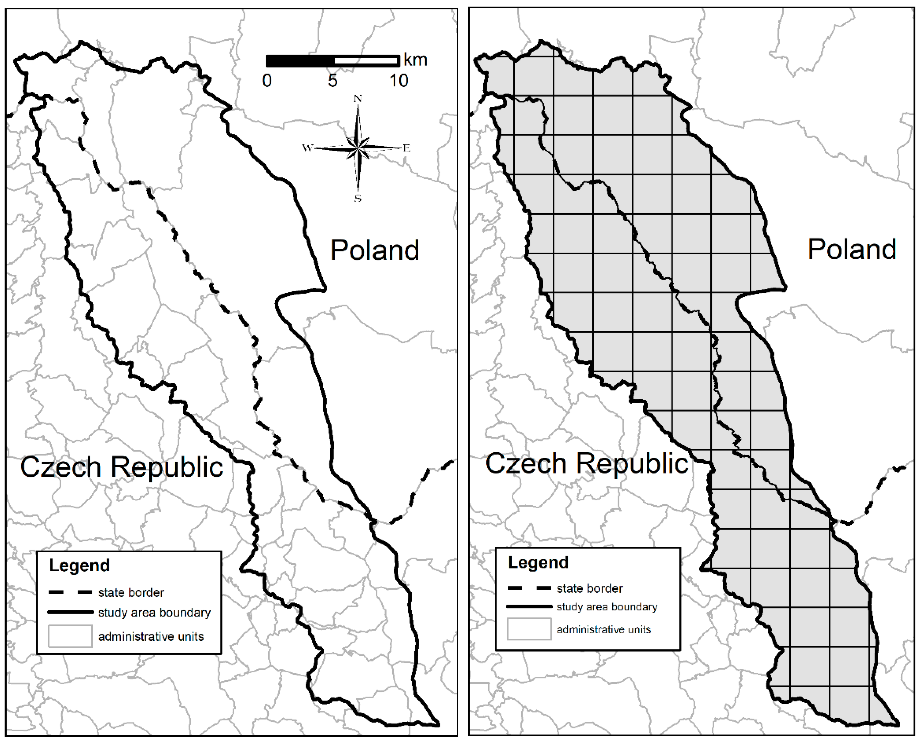
3.1. Study Area
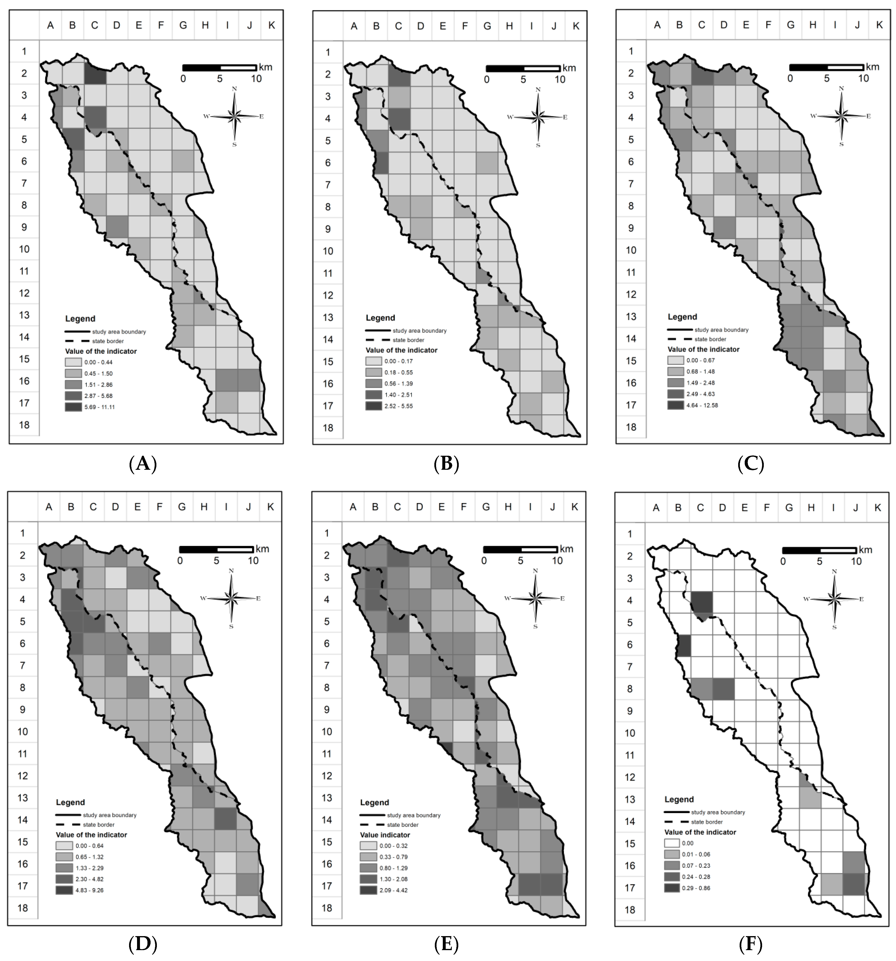
3.2. Square Grid
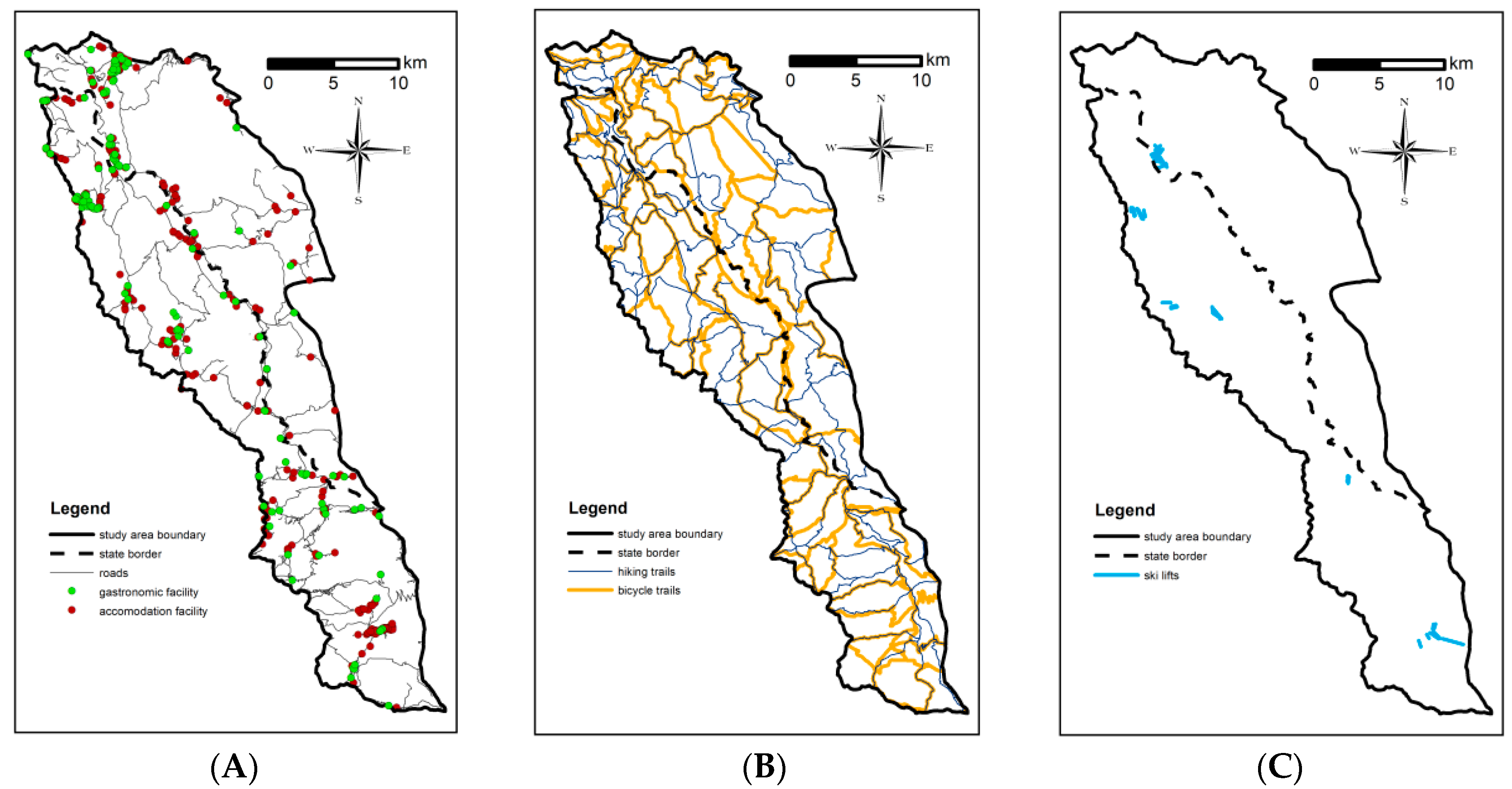
3.3. The Type of Analysed Tourism Infrastructure
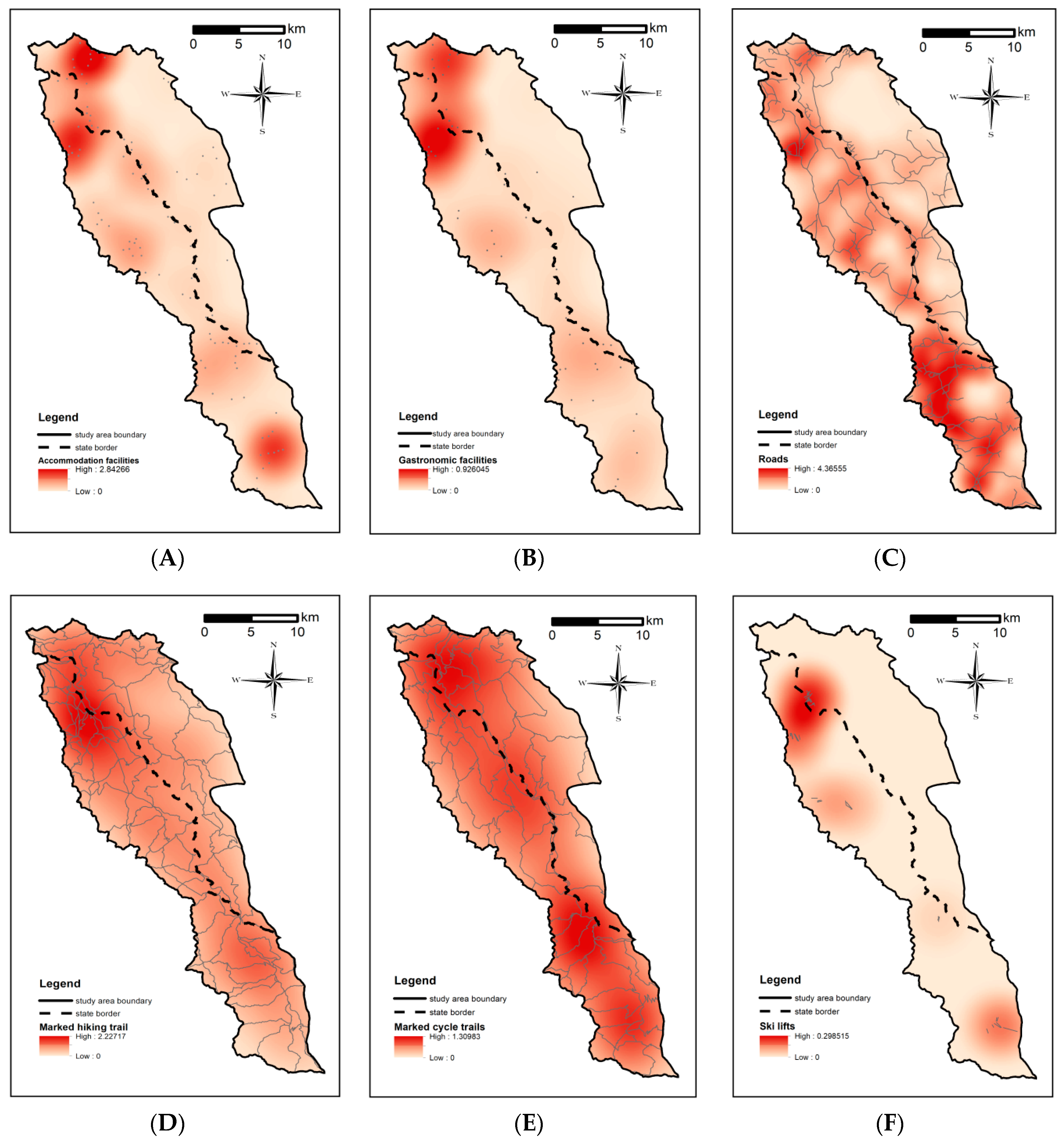
- Accommodation facilities (locations of hotels, motels, agritourism facilities, sanatoriums, private guest rooms, apartments, and campsites);
- Gastronomic facilities (locations of bars and restaurants, including restaurants in hotels open to people who are not hotel guests);
- Roads (length in km, paved public roads accessible to motorists);
- Hiking marked trails (length in km);
- Cycle tourist marked trails (length in km);
- Ski lifts (every type, length in km).
- Visit Duszniki (http://visitduszniki.pl, accessed on 26 May 2019),
- Lasówka in the heart of the Sudetes (http://lasowka.info/, accessed on 27 May 2019);
- Accommodations in the Czech Republic and Slovakia (https://www.ceskoslovensko.cz, accessed on 28 May 2019);
- The official tourism Internet portal of the Parubicko region in the Czech Republic https://www.czechy-wschodnie.info, accessed on 28 May 2019);
- The internet portal “Spalona” (http://www.spalona.com.pl/noclegi.php, accessed on 28 May 2019);
- The internet portal “E-turysta” (https://e-turysta.pl, accessed on 28 May 2019).
3.4. Methods for Calculating the Component Indicators and Final Synthetic Index
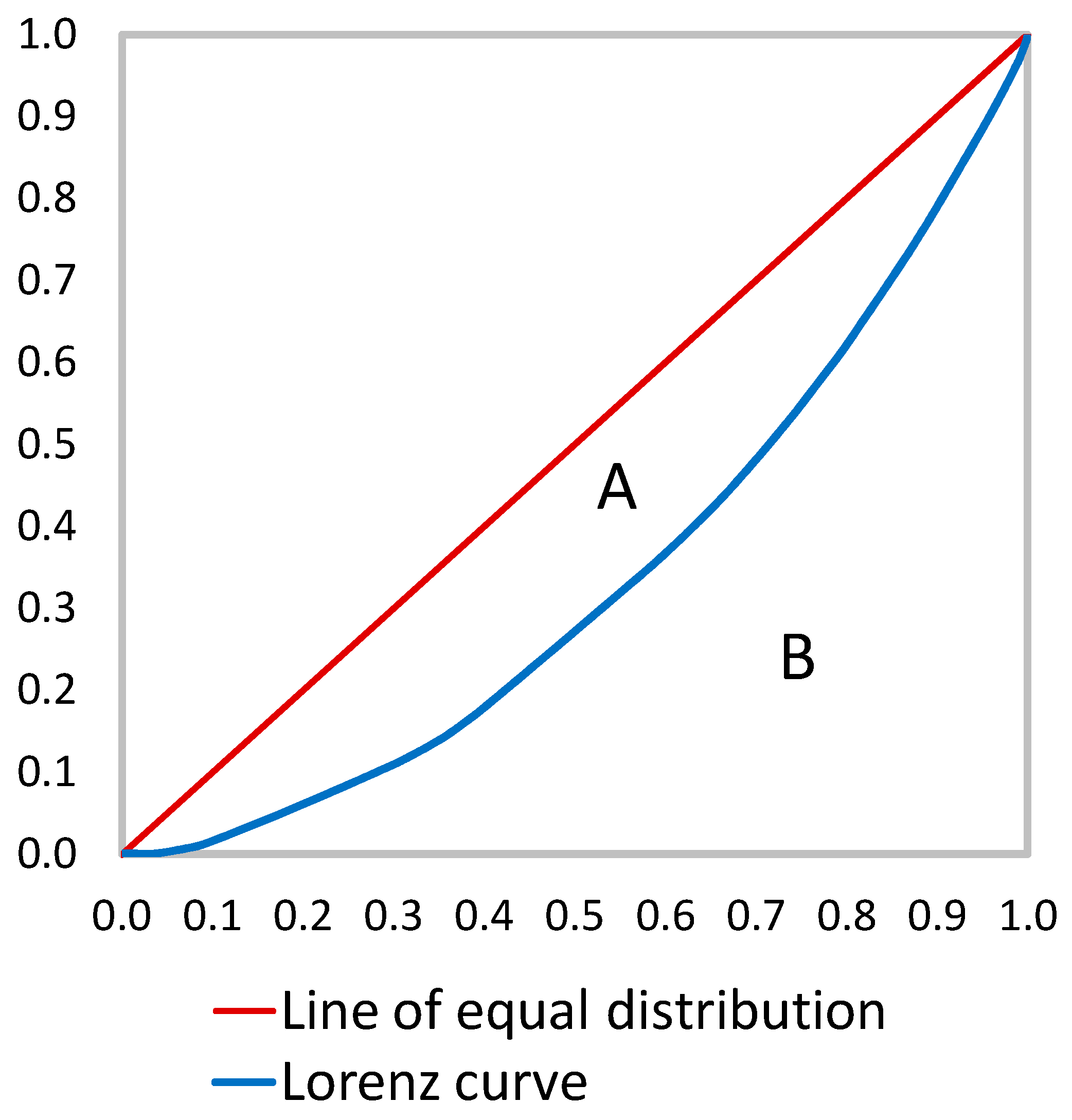
3.5. Analysis of Spatial Distribution
4. Results
4.1. Tourism Infrastructure in the Area of the Research
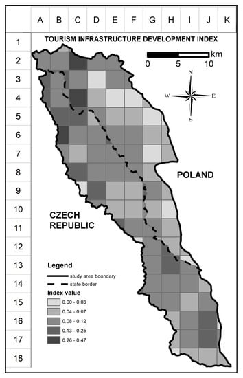
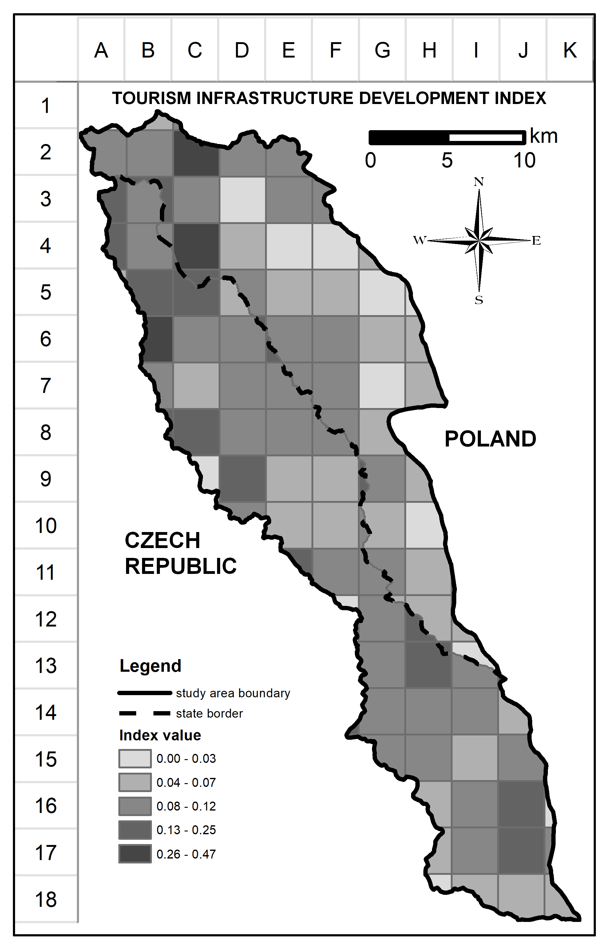
4.2. Synthetic Index of Tourism Infrastructure Development
5. Discussion
6. Summary and Conclusions
- (1)
- The use of geometric grid cells is particularly beneficial for the analysis and comparison of phenomena occurring in areas that have significantly different sizes of administrative or statistical units or are not internally divided into such units. In this case, data must be obtained from other sources, such as analogue maps, digital maps, satellite images, or field studies (hence, they are often used in ecological research and in cities that form a single administrative unit);
- (2)
- The advantage of using an artificial geometric grid is its greater readability for the end user compared to a typical choropleth map based on administrative units since the division of space is uniform;
- (3)
- Full geometric fields facilitate the calculation of density indices that can be used in multivariate analysis, such as HDI, thereby obtaining synthetic measures for the development of the studied phenomenon and considering the component indicators for the linear, point, and surface objects in one index;
- (4)
- The comparative analysis of features in two adjacent areas using grid methods experiences difficulties associated with the need to irregularly clip (trim) the geometric fields to the boundary of the study area, which is contrary to the principle of dividing the area into equal fields;
- (5)
- The hotspot KDE method enables one to determine the main clusters of examined infrastructure facilities but does not allow one to create synthetic development indicators for the entire studied area.
Author Contributions
Funding
Conflicts of Interest
References
- Więckowski, M. Tourism development in the borderlands of Poland. Geogr. Pol. 2010, 83, 67–81. [Google Scholar] [CrossRef] [Green Version]
- Prokkola, E.-K. Borders in tourism: The transformation of the Swedish–Finnish border landscape. Curr. Issues Tour. 2010, 13, 223–238. [Google Scholar] [CrossRef]
- Anisiewicz, R.; Palmowski, T. Small border traffic and cross-border tourism between Poland and the Kaliningrad Oblast of the Russian Federation. Quaest. Geogr. 2014, 33, 79–85. [Google Scholar] [CrossRef] [Green Version]
- Kladivo, P.; Ptáček, P.; Roubínek, P.; Ziener, K. Czech-Polish and Austrian-Slovenian borderland–similarities and differences of development and typology of regions. Morav. Geogr. Rep. 2012, 20, 48–63. [Google Scholar]
- Pászto, V.; Macků, K.; Burian, J.; Pánek, J.; Tuček, P. Capturing cross-border continuity: The case of the Czech-Polish borderland. Morav. Geogr. Rep. 2019, 27, 122–138. [Google Scholar] [CrossRef] [Green Version]
- Kołodziejczyk, K. Changes in the network of tourist trails in the border zones of the Czech Republic after entering the Schengen area. J. Mt. Sci. 2020, 17, 949–972. [Google Scholar] [CrossRef]
- Dołzbłasz, S. From Divided to Shared Spaces: Transborder Tourism in the Polish-Czech Borderlands. In Tourism and Geopolitics: Issues and Concepts from Central and Eastern Europe; Hall, D., Ed.; CABI: Boston, MA, USA, 2017; pp. 163–177. [Google Scholar]
- Furmankiewicz, M. Town-twinning as a factor generating international flows of goods and people–the example of Poland. Belgeo. Rev. Belg. De Géographie 2005, 1, 145–162. [Google Scholar] [CrossRef] [Green Version]
- Przybyła, K.; Kulczyk-Dynowska, A. Transformations of Tourist Functions in Urban Areas of the Karkonosze Mountains. IOP Conf. Ser. Mater. Sci. Eng. 2017, 245, 1–7. [Google Scholar] [CrossRef] [Green Version]
- Böhm, H.; Šmída, J. Borders on the old maps of Jizera Mountain. Misc. Geogr.-Reg. Stud. Dev. 2019, 23, 199–209. [Google Scholar] [CrossRef] [Green Version]
- Capello, R.; Caragliu, A.; Fratesi, U. Measuring border effects in European cross-border regions. Reg. Stud. 2018, 52, 986–996. [Google Scholar] [CrossRef]
- Slocum, T.A.; McMaster, R.B.; Kessler, F.C.; Howard, H.H. The Chorodot Map. In Thematic Cartography and Geographic Visualization; Pearson Prentice Hall: Upple Saddle River, NJ, USA, 2004. [Google Scholar]
- MacEachren, A.M.; DiBiase, D. Animated Maps of Aggregate Data: Conceptual and Practical Problems. Cartogr. Geogr. Inf. Syst. 1991, 18, 221–229. [Google Scholar] [CrossRef]
- Masot, A.N.; Alonso, G.C. The Rural Development Policy in Extremadura (SW Spain): Spatial Location Analysis of Leader Projects. ISPRS Int. J. Geo-Inf. 2018, 7, 1–16. [Google Scholar]
- Sklenicka, P.; Šímová, P.; Hrdinová, K.; Salek, M. Changing rural landscapes along the border of Austria and the Czech Republic between 1952 and 2009: Roles of political, socioeconomic and environmental factors. Appl. Geogr. 2014, 47, 89–98. [Google Scholar] [CrossRef]
- Burdziej, J. Using hexagonal grids and network analysis for spatial accessibility assessment in urban environments—A case study of public amenities in Toruń. Misc. Geogr.-Reg. Stud. Dev. 2019, 23, 99–110. [Google Scholar] [CrossRef] [Green Version]
- Ciok, S. Problematyka obszarów przygranicznych polski południowo-zachodniej. Studium społeczno-ekonomiczne. In Acta Universitatis Wratislaviensis No 1155; Państwowe Wydawnictwo Naukowe, Oddział Wrocławski: Wrocław, Poland, 1990. [Google Scholar]
- Kolejka, J.; Żyszkowska, W.; Batelková, K.; Ciok, S.; Dołzbłasz, S.; Kirchner, K.; Krejčí, T.; Raczyk, A.; Spallek, W.; Zapletalová, J. Permeability of Czech-Polish border using by selected criteria. Geogr. Tech. 2015, 10, 51–65. [Google Scholar]
- Latocha, A. Changes in the rural landscape of the Polish Sudety Mountains in the post-war period. Geogr. Pol. 2012, 85, 13–21. [Google Scholar] [CrossRef]
- Vaishar, A.; Dvořák, P.; Hubačíková, V.; Zapletalová, J. Contemporary development of peripheral parts of the Czech-Polish borderland: Case study of the Javorník area. Geogr. Pol. 2013, 86, 237–253. [Google Scholar] [CrossRef]
- Furmankiewicz, M.; Knieć, W.; Atterton, J. Rural governance in the new EU member states: The experience of the Polish LEADER+ Pilot Programme (2004–2008). In Governance in Transition; Buček, J., Ryder, A., Eds.; Springer Geography: Dordrecht, The Netherlands, 2015; pp. 133–153. [Google Scholar]
- Furmankiewicz, M.; Campbell, A. From Single-Use Community Facilities Support to Integrated Sustainable Development: The Aims of Inter-Municipal Cooperation in Poland, 1990–2018. Sustainability 2019, 11, 5890. [Google Scholar] [CrossRef] [Green Version]
- Dołzbłasz, S. A network approach to transborder cooperation studies as exemplified by Poland’s eastern border. Geogr. Pol. 2018, 91, 63–76. [Google Scholar] [CrossRef] [Green Version]
- Böhm, H.; Drápela, E. Cross-border cooperation as a reconciliation tool: Example from the East Czech-Polish borders. Reg. Fed. Stud. 2017, 27, 305–319. [Google Scholar] [CrossRef]
- Czetwertyński-Sytnik, L.; Kozioł, E.; Mazurski, K.R. Settlement and sustainability in the Polish Sudetes. GeoJournal 2000, 50, 273–284. [Google Scholar] [CrossRef]
- Dołzbłasz, S. Symmetry or asymmetry? Cross-border openness of service providers in Polish-Czech and Polish-German border towns. Morav. Geogr. Rep. 2015, 23, 2–12. [Google Scholar] [CrossRef] [Green Version]
- Mun, S.-I.; Nakagawa, S. Pricing and investment of cross-border transport infrastructure. Reg. Sci. Urban Econ. 2010, 40, 228–240. [Google Scholar] [CrossRef] [Green Version]
- Holly, W.; Nekvapil, J.; Scherm, I.; Tišerová, P. Unequal neighbours: Coping with asymmetries. J. Ethn. Migr. Stud. 2003, 29, 819–834. [Google Scholar] [CrossRef]
- Furmankiewicz, M.; Buryło, K.; Dołzbłasz, S. From service areas to empty transport corridors? The impact of border openings on service and retail facilities at Polish-Czech border crossings. Morav. Geogr. Rep. 2020, 28, 136–151. [Google Scholar]
- Rietveld, P. Barrier Effects of Borders: Implications for Border Crossing Infrastructures. Eur. J. Transp. Infrastruct. Res. 2012, 12, 150–166. [Google Scholar]
- Hełdak, M.; Bykowa, E. Construction of public roads at the meeting point of different legislation systems. J. Ecol. Eng. 2017, 18, 86–94. [Google Scholar] [CrossRef]
- Forest, P. Transferring bulk water between Canada and the United States: More than a century of transboundary inter-local water supplies. Geoforum 2012, 43, 14–24. [Google Scholar] [CrossRef]
- Lamparska, M. The post-industrial tourist route in Poland and the Czech Republic borderland. Acta Geogr. Sil. 2016, 23, 57–66. [Google Scholar]
- Furmankiewicz, M. International Cooperation of Polish Municipalities: Directions and Effects. Tijdschr. Voor Econ. En Soc. Geogr. 2007, 98, 349–359. [Google Scholar] [CrossRef]
- Ciok, S.; Raczyk, A. Implementation of the EU Community Initiative INTERREG III A at the Polish-German border: An attempt at evaluation. In Cross-border Governance and Sustainable Spatial Development: Mind the Gaps! Leibenath, M., Korcelli-Olejniczak, E., Knippschild, R., Eds.; Springer: Berlin, Germany, 2008; pp. 33–47. [Google Scholar]
- Stacherzak, A.; Hełdak, M. Borough Development Dependent on Agricultural, Tourism, and Economy Levels. Sustainability 2019, 11, 415. [Google Scholar] [CrossRef] [Green Version]
- Rogalewski, O. Zagospodarowanie Turystyczne; Wydawnictwa Szkolne i Pedagogiczne: Warszawa, Poland, 1979. [Google Scholar]
- United Nations World Tourism Organization. Glossary of Tourism Terms; United Nations World Tourism Organization: Madrid, Spain, 2008. [Google Scholar]
- Konakoglu, S.S.K.; Hełdak, M.; Kurdoglu, B.C.; Wysmułek, J. Evaluation of Sustainable Development of Tourism in Selected Cities in Turkey and Poland. Sustainability 2019, 11, 2552. [Google Scholar] [CrossRef] [Green Version]
- Jovanović, S.; Ilić, I. Infrastructure as Important Determinant of Tourism Development in the Countries of Southeast Europe. Ecoforum 2016, 5, 288–294. [Google Scholar]
- Mandić, A.; Mrnjavac, Ž.; Kordić, L. Tourism infrastructure, recreational facilities and tourism development. Tour. Hosp. Manag. 2018, 24, 41–62. [Google Scholar] [CrossRef]
- Panasiuk, A. Tourism infrastructure as a determinant of regional development. Ekon. Ir Vadyb. Aktualijos Ir Perspekt. 2007, 1, 212–215. [Google Scholar]
- Kulczyk-Dynowska, A.; Stacherzak, A. Selected Elements of Technical Infrastructure in Municipalities Territorially Connected with National Parks. Sustainability 2020, 12, 4015. [Google Scholar] [CrossRef]
- Przybyła, K.; Kachniarz, M.; Kulczyk-Dynowska, A.; Ramsey, D. The impact of changes in administrative status on the tourist functions of cities: A case study from Poland. Econ. Res.-Ekon. Istraživanja 2019, 32, 578–603. [Google Scholar] [CrossRef]
- Kozak, M.W. Innovation, Tourism and Destination Development: Dolnośląskie Case Study. Eur. Plan. Stud. 2014, 22, 1604–1624. [Google Scholar] [CrossRef]
- Pijet-Migoń, E.; Migoń, P. Promoting and Interpreting Geoheritage at the Local Level‒Bottom-up Approach in the Land of Extinct Volcanoes, Sudetes, SW Poland. Geoheritage 2019, 11, 1227–1236. [Google Scholar] [CrossRef] [Green Version]
- The European Parliament and the Council of the European Union. Directive 2007/2/EC of the European Parliament and of the Council of 14 March 2007 establishing an Infrastructure for Spatial Information in the European Community (INSPIRE). Off. J. Eur. Union 2007, L108, 1. [Google Scholar]
- Bregt, A.K.; Smits, P.C. INSPIRE (Infrastructure for Spatial Information in Europe). Geo-Info 2004, 1, 460–462. [Google Scholar]
- Kazak, J.; Szewrański, S. The Use of Geoinformation in Land Acquisition for Road Developments. Real Estate Manag. Valuat. 2014, 22, 32–38. [Google Scholar] [CrossRef] [Green Version]
- Olszewski, R.; Gotlib, D.; Iwaniak, A. GIS: Obszary Zastosowań; Wydawnictwo Naukowe PWN: Warszawa, Poland, 2007. [Google Scholar]
- Ustawa z Dnia 4 Marca 2010 r. o Infrastrukturze Informacji Przestrzennej; No 76 Pos. 489; Dziennik Ustaw: Warszawa, Poland, 2010.
- Andrzejewska, M.; Jała, Z.; Rusztecka, M. Harmonizacja danych przestrzennych dotyczących transgranicznego obszaru chronionego na przykładzie Karkonoskiego Parku Narodowego oraz Krkonosského Národního Parku w ramach projektu “Karkonosze w INSPIRE–wspólny GIS dla ochrony przyrody”. Rocz. Geomatyki 2011, 9, 7–13. [Google Scholar]
- Máliková, L.; Klobučník, M.; Bačík, V.; Spišiak, P. Socio-economic changes in the borderlands of the Visegrad Group (V4) countries. Morav. Geogr. Rep. 2014, 23, 26–37. [Google Scholar] [CrossRef]
- Smolarski, M.; Jurkowski, W.; Raczyk, A. Bus and train connections between towns in Lower Silesia under different operational models: Competition or complementarity? Morav. Geogr. Rep. 2019, 27, 31–40. [Google Scholar]
- Czerwiński, J. Problemy turystyki i wypoczynku w Sudetach. In Przestrzenne problemy rozwoju społeczno-gospodarczego Sudetów. Acta Universitatis Wratislaviensis No 1343. Studia Geograficzne 58; Łoboda, J., Ed.; Wydawnictwo Uniwersytetu Wrocławskiego: Wrocław, Poland, 1993. [Google Scholar]
- Ciok, S. Niekorzystne tendencje zmian w rozwoju społeczno-gospodarczym Sudetów. Czas. Geogr. 1988, 59, 171–183. [Google Scholar]
- Poštolka, V.; Šmída, J. Źródła informacji o środowisku województwa libereckiego i Euroregionu Neisse-Nisa-Nysa. In Problemy współpracy na rzecz ekorozwoju Sudetów; Furmankiewicz, M., Jadczyk, P., Eds.; Muzeum Przyrodnicze w Jeleniej Górze: Jelenia Góra, Poland, 2006. [Google Scholar]
- Bartniczak, B. Sustainable Development in the Polish-Czech Cross Border Area-Indicators Analysis. In Hradec Economic Days Vol. 9(1). Double-Blind Peer-Reviewed Proceedings Part. I of the International Scientific Conference Hradec Economic Days 2019; Jedlička, P., Soukal, I., Marešová, P., Eds.; University of Hradec Králové: Hradec Králové, Czech Republic, 2019; pp. 19–28. [Google Scholar]
- Poštolka, V.; Šmída, J.; Dítĕtová, V. Wybrane problemy opracowania strategii zrównoważonego rozwoju województwa libereckiego i Euroregionu Neisse-Nisa-Nysa. In Problemy współpracy na rzecz ekorozwoju Sudetów; Furmankiewicz, M., Jadczyk, P., Eds.; Muzeum Przyrodnicze w Jeleniej Górze: Jelenia Góra, Poland, 2006; pp. 49–70. [Google Scholar]
- Kołodziejczyk, K. Rozwój sieci szlaków turystycznych wzdłuż granicy polsko-czeskiej w Sudetach w latach 1945–2013. Prz. Geogr. 2014, 136, 81–101. [Google Scholar]
- Potocki, J.; Kachniarz, M.; Piepiora, Z. Sudetes-cross-border region? In The International Conference Hradec Economic Days 2014. Economic Development and Management of Regions. Peer-Reviewed Conference Proceedings; Part, V., Jedlicka, P., Eds.; Gaudeamus: Hradec Králové, Czech Republic, 2014; pp. 191–200. [Google Scholar]
- Kachniarz, M.; Szewranski, S.; Kazak, J. The Use of European Funds in Polish and Czech Municipalities. A Study of the Lower Silesia Voivodship and Hradec Kralove Region. IOP Conf. Ser. Mater. Sci. Eng. 2019, 471, 112047. [Google Scholar] [CrossRef]
- Kurowska-Pysz, J.; Szczepańska-Woszczyna, K. The Analysis of the Determinants of Sustainable Cross-Border Cooperation and Recommendations on Its Harmonization. Sustainability 2017, 9, 2226. [Google Scholar] [CrossRef] [Green Version]
- Furmankiewicz, M.; Potocki, J.; Kazak, J. Land-Use Conflicts in the Sudetes, Poland. IOP Conf. Ser. Mater. Sci. Eng. 2019, 471, 092033. [Google Scholar] [CrossRef]
- Mazurski, K.R. Environmental problems in the Sudetes, Poland. GeoJournal 1999, 46, 271–277. [Google Scholar] [CrossRef]
- Szmytkie, R.; Tomczak, P. Revival of rural settlements in Kłodzko Land. Geogr. Pol. 2017, 90, 319–333. [Google Scholar] [CrossRef] [Green Version]
- Krajewski, P.; Solecka, I.; Mrozik, K. Forest Landscape Change and Preliminary Study on Its Driving Forces in Ślęża Landscape Park (Southwestern Poland) in 1883–2013. Sustainability 2018, 10, 4526. [Google Scholar] [CrossRef] [Green Version]
- Migoń, P.; Latocha, A. Human impact and geomorphic change through time in the Sudetes, Central Europe. Quat. Int. 2018, 470, 194–206. [Google Scholar] [CrossRef]
- Bródka, S.; Macias, A. Etapy oceny środowiska przyrodniczego oraz ich znaczenie w procesie planistycznym (Stages in the assessment of the natural environment and their significance in the planning process). In Waloryzacja środowiska przyrodniczego w planowaniu przestrzennym (Environmental Assessment in Physical Planning); Kistowski, M., Korwel-Lejkowska, B., Eds.; Fundacja Rozwoju Uniwersytetu Gdańskiego: Gdańsk, Poland, 2007; pp. 61–75. [Google Scholar]
- EUROSTAT. History of NUTS. Available online: https://ec.europa.eu/eurostat/web/nuts/history (accessed on 15 March 2020).
- Carr, D.B.; Olsen, A.R.; White, D. Hexagon Mosaic Maps for Display of Univariate and Bivariate Geographical Data. Cartogr. Geogr. Inf. Syst. 1992, 19, 228–236. [Google Scholar] [CrossRef]
- Birch, C.P.D.; Oom, S.P.; Beecham, J.A. Rectangular and hexagonal grids used for observation, experiment and simulation in ecology. Ecol. Model. 2007, 206, 347–359. [Google Scholar] [CrossRef]
- De Oliveira, M.G.; De Souza Baptista, C. GeoSTAT–A system for visualization, analysis and clustering of distributed spatio-temporal data. In Proceedings of the XIII GEOINFO, Campos do Jordão, Brazil, 25–27 November 2012; pp. 108–119. [Google Scholar]
- Radermacher, W. Population Grid Statistics from Hybrid Sources. Real. Datos Y Espac.–Rev. Int. De Estadística Y Geogr. 2012, 3, 48–59. [Google Scholar]
- Nistor, M.-M.; Rahardjo, H.; Satyanaga, A. Development Assessment of the Singapore Land: A Gis Spatial-Temporal Approach Based on Land Cover Analysis. Geogr. Tech. 2019, 14, 60–73. [Google Scholar] [CrossRef] [Green Version]
- Wang, L.; Fan, H.; Wang, Y. Site Selection of Retail Shops Based on Spatial Accessibility and Hybrid BP Neural Network. ISPRS Int. J. Geo-Inf. 2018, 7, 202. [Google Scholar] [CrossRef] [Green Version]
- Uher, V.; Gajdoš, P.; Snášel, V. Searching of Circular Neighborhoods in the Square and Hexagonal Regular Grids. In Intelligent Data Analysis and Processing; Pan, J.-S., Snášel, V., Sung, T.-W., Wang, X.D., Eds.; Springer International Publishing AG: Cham, Switzerland, 2016; pp. 121–129. [Google Scholar]
- Battersby, S.E.; Strebea, D.; Finn, M.P. Shapes on a plane: Evaluating the impact of projection distortion on spatial binning. Cartogr. Geogr. Inf. Sci. 2016, 44, 410–421. [Google Scholar] [CrossRef]
- Klimczak, H. (Ed.) Analizy przestrzenne w badaniach warunków gospodarowania na obszarach wiejskich województwa dolnośląskiego (Spatial Analyses in Studies over Development Conditions in the Rural Areas on the Example of Dolnośląskie Voivodship); Wydawnictwo Uniwersytetu Przyrodniczego we Wrocławiu: Wrocław, Poland, 2008. [Google Scholar]
- Jelinski, D.E.; Wu, J. The modifiable areal unit problem and implications for landscape ecology. Landsc. Ecol. 1996, 11, 129–140. [Google Scholar] [CrossRef]
- Swift, A.; Liu, L.; Uber, J. Reducing MAUP bias of correlation statistics between water quality and GI illness. Comput. Environ. Urban. Syst. 2008, 32, 134–148. [Google Scholar] [CrossRef]
- Fotheringham, A.S.; Wong, D.W.S. The modifiable areal unit problem in multivariate statistical analysis. Environ. Plan. A 1991, 23, 1025–1044. [Google Scholar] [CrossRef]
- Wang, L.; Fan, H.; Gong, T. The Consumer Demand Estimating and Purchasing Strategies Optimizing of FMCG Retailers Based on Geographic Methods. Sustainability 2018, 10, 466. [Google Scholar] [CrossRef] [Green Version]
- Zhong, A.; Wu, Y.; Nie, K.; Kang, M. Using Local Toponyms to Reconstruct the Historical River Networks in Hubei Province, China. ISPRS Int. J. Geo-Inf. 2020, 9, 318. [Google Scholar] [CrossRef]
- Pieniążek, M.; Szejgiec, B.; Zych, M.; Ajdyn, A.; Nowakowska, G. Graficzna Prezentacja Danych Statystycznych: Wykresy, Mapy, GIS; Główny Urząd Statystyczny, Departament Badań Regionalnych i środowiska: Warszawa, Poland, 2014. [Google Scholar]
- Iwaniak, A.; Leszczuk, M.; Strzelecki, M.; Harvey, F.; Kaczmarek, I. A novel approach for publishing linked open geodata from national registries with the use of semantically annotated context dependent web pages. ISPRS Int. J. Geo-Inf. 2017, 6, 252. [Google Scholar] [CrossRef] [Green Version]
- Bednarek-Szczepańska, M.; Więckowski, M. Możliwości pozyskania danych na temat zagospodarowania i ruchu turystycznego oraz propozycje wskaźników. Biul. KPZK PAN 2013, 252, 143–163. [Google Scholar]
- Anand, S.; Sen, A.K. Human Development Index: Methodology and Measurement; Human Development Report Office, United Nations Development Programme: New York, NY, USA, 1994. [Google Scholar]
- Szewrański, S.; Bochenkiewicz, M.; Kachniarz, M.; Kazak, J.K.; Sylla, M.; Świąder, M.; Tokarczyk-Dorociak, K. Location support system for energy clusters management at regional level. IOP Conf. Ser. Earth Environ. Sci. 2019, 354, 012021. [Google Scholar] [CrossRef]
- Ciok, S.; Dołzbłasz, S.; Raczyk, A. Dolny Śląsk: Problemy Rozwoju Regionalnego (Lower Silesia: Problems of Regional Development); Wydawnictwo Uniwersytetu Wrocławskiego: Wrocław, Poland, 2006. [Google Scholar]
- Kovacevic, M. Review of HDI Critiques and Potential Improvements. Hum. Dev. Res. Pap. 2010, 33, 1–44. [Google Scholar]
- Zahran, E.-S.M.M.; Tan, S.J.; Tan, E.H.A.; Mohamad’ Asri Putra, N.A.A.B.; Yap, Y.H.; Abdul Rahman, E.K. Spatial analysis of road traffic accident hotspots: Evaluation and validation of recent approaches using road safety audit. J. Transp. Saf. Secur. 2019, 1–30. [Google Scholar] [CrossRef]
- Chang, K.-T. Introduction to Geographic Information Systems, 9th ed.; McGraw Hill: New York, NY, USA, 2019. [Google Scholar]
- Kalinic, M.; Krisp, J.M. Kernel Density Estimation (KDE) vs. Hot-Spot Analysis-Detecting Criminal Hot Spots in the City of San Francisco. In Geospatial Technologies for All: Short Papers, Posters and Poster Abstracts of the 21th AGILE Conference on Geographic Information Science, Lund University, Lund, Sveden, 12–15 June 2018; Mansourian, A., Pilesjö, P., Harrie, L., van Lammeren, R., Eds.; Lund University: Lund, Sveden, 2018; pp. 1–5. [Google Scholar]
- Lin, Y.-P.; Chu, H.-J.; Wu, C.-F.; Chang, T.-K.; Chen, C.-Y. Hotspot Analysis of Spatial Environmental Pollutants Using Kernel Density Estimation and Geostatistical Techniques. Int. J. Environ. Res. Public Health 2011, 8, 75–88. [Google Scholar] [CrossRef] [PubMed]
- Gastwirth, J.L. A General Definition of the Lorenz Curve. Econometrica 1971, 39, 1037–1039. [Google Scholar] [CrossRef]
- Saha, D.; Kemanian, A.R.; Montes, F.; Gall, H.; Adler, P.R.; Rau, B.M. Lorenz Curve and Gini Coefficient Reveal Hot Spots and Hot Moments for Nitrous Oxide Emissions. J. Geophys. Res. Biogeosciences 2018, 193–206. [Google Scholar] [CrossRef] [Green Version]
- Stacherzak, A.; Hájek, L.; Hełdak, M. Changes in the Use of Agricultural Land in Poland and Czech Republic. J. Ecol. Eng. 2019, 20, 211–221. [Google Scholar] [CrossRef]
- Carlino, G.; Kerr, W.R. Agglomeration and Innovation. In Handbook of Regional and Urban Economics; Duranton, G., Henderson, J.V., Strange, W.C., Eds.; Elsevier: Amsterdam, The Netherlands, 2015; pp. 349–404. [Google Scholar]
- Bellù, L.G.; Liberati, P. Charting Income Inequality. In The Lorenz Curve; Food and Agriculture Organization of the United Nations, FAO: Rome, Italy, 2005. [Google Scholar]
- Alonso-Villar, O. Measuring concentration: Lorenz curves and their decompositions. Ann. Reg. Sci. 2011, 47, 451–475. [Google Scholar] [CrossRef]
- Eberhardt, P. Political and administrative boundaries of the German state in the 20th century. Geogr. Pol. 2017, 90, 335–350. [Google Scholar] [CrossRef]
- Oleszek, J. Significant changes in the character and form of villages in the Złote Góry Mountains boundary region (Poland). Morav. Geogr. Rep. 2007, 15, 37–43. [Google Scholar]
- Hełdak, M.; Kempa, O. Current demographic changes in rural areas of south-western Poland, 1988–2002. Morav. Geogr. Rep. 2007, 15, 25–30. [Google Scholar]
- Ciok, S. Interreg IIIA programme in countries of Central and Eastern Europe. Geopolit. Stud. 2006, 14, 17–26. [Google Scholar]
- Sechi, L.; Moscarelli, R.; Pileri, P. Planning tourist infrastructures to regenerate marginalised territories: The study case of North Sardinia, Italy. City Territ. Archit. 2020, 7, 1–12. [Google Scholar] [CrossRef]
- Kałamucki, K.; Kamińska, A.; Buk, D. Spatial aspects of the research on tourist infrastructure with the use of the cartographic method on the basis of Roztoczański National Park. Ann. Univ. Mariae Curie-Sklodowska. Sect. B 2012, 67, 245–261. [Google Scholar] [CrossRef] [Green Version]


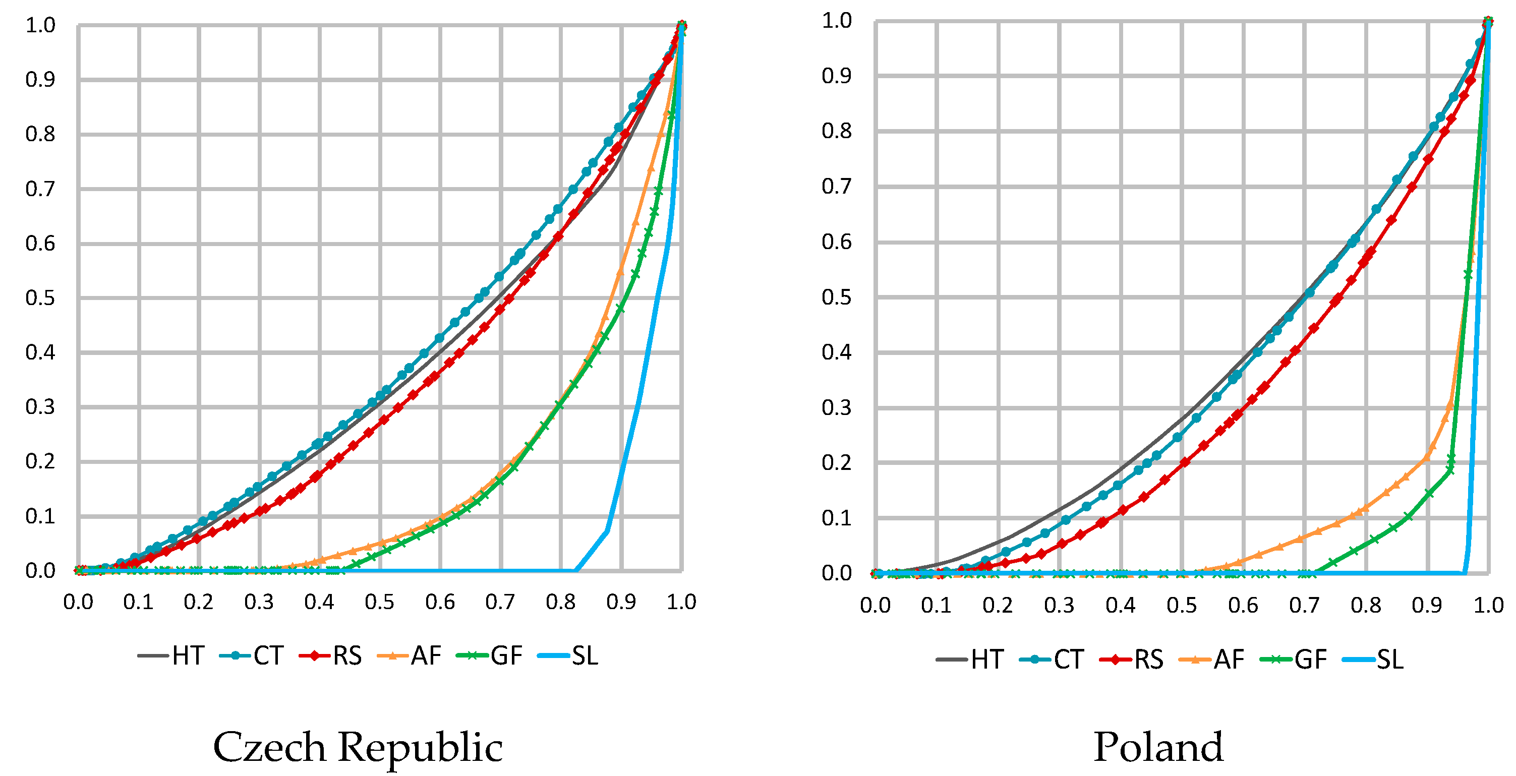
| Study Area | HT | CT | RS | AF | GF | SL |
|---|---|---|---|---|---|---|
| Czech Republic | 0.29 | 0.25 | 0.33 | 0.67 | 0.70 | 0.90 |
| Poland | 0.31 | 0.34 | 0.42 | 0.84 | 0.89 | 0.96 |
© 2020 by the authors. Licensee MDPI, Basel, Switzerland. This article is an open access article distributed under the terms and conditions of the Creative Commons Attribution (CC BY) license (http://creativecommons.org/licenses/by/4.0/).
Share and Cite
Jędruch, M.; Furmankiewicz, M.; Kaczmarek, I. Spatial Analysis of Asymmetry in the Development of Tourism Infrastructure in the Borderlands: The Case of the Bystrzyckie and Orlickie Mountains. ISPRS Int. J. Geo-Inf. 2020, 9, 470. https://doi.org/10.3390/ijgi9080470
Jędruch M, Furmankiewicz M, Kaczmarek I. Spatial Analysis of Asymmetry in the Development of Tourism Infrastructure in the Borderlands: The Case of the Bystrzyckie and Orlickie Mountains. ISPRS International Journal of Geo-Information. 2020; 9(8):470. https://doi.org/10.3390/ijgi9080470
Chicago/Turabian StyleJędruch, Michalina, Marek Furmankiewicz, and Iwona Kaczmarek. 2020. "Spatial Analysis of Asymmetry in the Development of Tourism Infrastructure in the Borderlands: The Case of the Bystrzyckie and Orlickie Mountains" ISPRS International Journal of Geo-Information 9, no. 8: 470. https://doi.org/10.3390/ijgi9080470