
Abstract
The determination of deformation parameters of rock material is an essential part of any design in rock mechanics. The goal of this paper is to show, that there is a relationship between static and dynamic modulus of elasticity (E), modulus of rigidity (G) and bulk modulus (K). For this purpose, different data on igneous, sedimentary and metamorphic rocks, all of which are widely used as construction materials, were collected and analyzed from literature. New linear and nonlinear relationships have been proposed and results confirmed a strong correlation between static and dynamic moduli of rock species. According to rock types, for igneous rocks, the best correlation between static and dynamic modulus of elasticity (E) were nonlinear logarithmic and power ones; for sedimentary rocks were linear and for metamorphic rocks were nonlinear logarithmic and power correlation. Moreover, with respect to different published linear correlations between static modulus of elasticity (Estat) and dynamic modulus of elasticity (Edyn), an interesting correlation for rock material constants was established. It was found that the static modulus of elasticity depends on the dynamic modulus only with one parameter formula.
1 Introduction
An accurate estimate of geomechanical properties of rocks is crucial for almost any form of design and analysis in geomechanical projects. The strength and deformation behavior of rocks have been studied by many authors Xiong et al. (2019), Yang et al. (2016), Zhao et al. (2017), Ranjith et al. (2004), Rahimi and Nygaard (2018), Davarpanah et al. (2019) and Berezovski and Ván (2017). Among these properties modulus of elasticity (E), modulus of rigidity (G) and bulk modulus (K) are the basic parameters used in rock engineering. There are two common methods to calculate the moduli: destructive and non-destructive procedures. In the destructive one, moduli are calculated from the stress–strain curves of the rock material. This is characteristic of the modulus of elasticity. For the non-destructive one, the most common method is an ultrasonic test, measuring both longitudinal and shear wave velocities.
Measuring the longitudinal and shear wave velocities, the dynamic elastic material parameters for isotropic and ideal elastic rocks are calculated with the help of the following formula (Martinez-Martinez et al. 2012):
where Edyn = dynamic modulus of elasticity, GPa, Gdyn = dynamic modulus of rigidity, GPa, Kdyn = dynamic bulk modulus, GPa, \({\text{J}}_{\text{dynamic}} = {\text{dynamic}}\;{\text{Poisso's}}\;{\text{ratio}}\), \(\rho = {\text{density}},\frac{\text{g}}{{{\text{cm}}^{ 3} }}\),\(V_{S} = {\text{shearvelocity}},\;{\text{km/s}}\), \(V_{P} = {\text{longitudinal}}\;{\text{infinite}}\;{\text{medium}}\;{\text{velocity}},{\text{km/s}}\).
The Young’s modulus obtained from the compression (destructive) test is called the static elastic modulus (Estat). The International Society for Rock Mechanics (ISRM) suggests three standard methods for its determination (Ulusay and Hudson 2007). They are as followings:
Tangent Young’s modulus Etan—at fixed percentage of ultimate stress. This is defined as the slope of a line tangent to the stress–strain curve at a fixed percentage of the ultimate strength (Fig. 1a);
Fig. 1 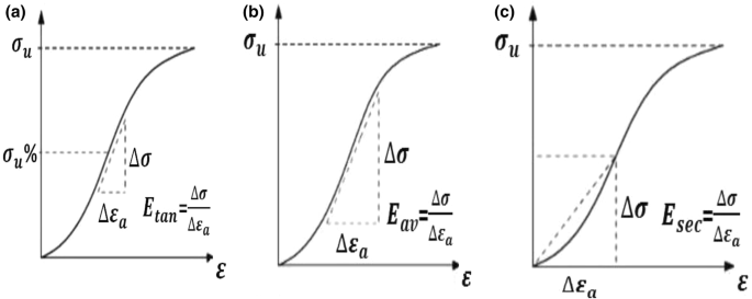
a Tangent Young’s modulus Etan, b Average Young’s modulus Eav, c Secant Young’s modulus Esec
Average Young’s modulus Eav—of the straight-line part of a curve. The elastic modulus is defined as the slope of the straight-line part of the stress–strain curve for the given test (Fig. 1b);
Secant Young’s modulus Esec—at a fixed percentage of ultimate stress. It is defined as the slope of the line from the origin (usually point (0; 0)) to some fixed percentage of ultimate strength, usually 50% (Fig. 1c). In this paper, the secant static modulus has been calculated following ASTM D 3148-69 (1996).

The difference between dynamic (\(E_{dyn}\)) and static (\(E_{stat}\)) Young’s Modulus for rocks has been addressed widely in rock engineering (van Heerden 1977; Lama and Vutukuri 1978; Barton 2006). Ratios for \(E_{dyn}\)/\(E_{stat}\) are typically in the range from 1 to 2 (Eissa and Kazi 1988).
Generally, the dynamic modulus of elasticity is slightly higher than the static value (Zhang 2006; Stacey et al. 1987; Al-Shayea 2004; Ide 1936; Kolesnikov 2009; Vanheerden 1987). The discrepancies between the dynamic and static elastic moduli have been widely attributed to microcracks and pores in the rocks. Figure 2 shows the ratio of dynamic elastic modulus to static elastic modulus compiled by Stacey et al. (1987). The ratio varies between about 1 and 3.

(Stacey et al. 1987)
Comparison of static and dynamic elastic modulus
In other research (Martinez-Martinez et al. 2012) conducted a laboratory experiment on ten different carbonate rocks quarried in Spain and received the following diagram (Fig. 3). As shown, for the majority of cases dynamic (\(E_{dyn}\)) Young’s Modulus is higher than static (\(E_{stat}\)) Young’s Modulus.

(Martinez–Martinez et al. 2012)
Relationship between Edyn and Estat in the studied samples. The straight red line corresponds to the ideal ratio \(\frac{{E_{dyn} }}{{E_{stat} }}\) = 1.
The rocks consist of homogeneous limestones, low anisotropic travertines, limestones and dolostones with abundant stylolites, veins and fissures. Ultrasonic waves were measured using non-polarised Panametric transducers (1 MHz), a precise ultrasonic device consisting of signal emitting– receiving equipment and an oscilloscope (TDS 3012BTektronix) (Martinez-Martinez et al. 2012) (Fig. 4).

Plot of the relationship between the measured static and dynamic modulus of elasticity (Estat = a Edyn − b)
Types of rocks are denoted below the picture and can be described as following. Blanco Alconera (BA): white crystalline limestone. Piedra de Colmenar (PdC): grey and white lacustrine fossiliferous limestone (99% calcite). Travertino Amarillo (TAm): porous layered limestone Travertino Rojo (TR): porous layered limestone. Gris Macael (GM): grey calcite marble.Blanco Tranco (BT): white homogeneous calcite marble. Amarillo Triana (AT): yellow dolomite marble.Crema Valencia (CV): cream micritic limestone (99% calcite). Rojo Cehegín (RC): micritic limestone. Marrón Emperador (ME): brown brecciated dolostone.
2 Empirical relationships between dynamic and static Young’s modulus
There are several relationships between the static and dynamic Young’s moduli (Belikov et al. 1970; King 1983; Eissa and Kazi 1988; McCann and Entwisle 1992; Eissa and Kazi 1988; Christaras et al. 1994; Nur and Wang 1999; Brotons et al. 2014, 2016; Małkowskia et al. 2018). These equations can be divided into the following groups:
Linear
Non-linear: Logarithmic (power-law) and polynomial
2.1 Linear relationships
Up to now, several linear relationships have been established between the dynamic and the static Young’s modulus. The following form was used:
where a and b are material parameters. These values are summarized in Table 1.
2.2 Non-linear relationships
Some published papers use a logarithmic relationship. Analyzing the measured data, they suggest the following formula between the dynamic and the static Young’s modulus:
The values of Estat, and Edyn are expressed in GPa while that of ρbulk in g/cm3. Here c and d are material constants (the published values are summarized in Table 2).
These equations can be rewritten to the following form:
where the parameters are presented in Table 3.
The power-law relation (7) was suggested in other researches, too (see Table 4). E.g. according to the data of Ohen (2003). the dynamic Young’s modulus is about 18 times the static Young’s modulus (Peng and Zhang 2007).
From ultrasonic test data of 600 core samples in the Gulf of Mexico, Lacy (1997) obtained the following polynomial correlation for sandstones (Peng and Zhang 2007):
A similar connection exists for shales and sedimentary rocks (Horsrud 2001; see Table 5).
3 Data analysis
For this study, 40 samples of different types of rocks from the literature were analyzed (Lama and Vutukuri 1978). Data were classified according to rock types and the relationship between dynamic and static constants was investigated in Table 6. Also, the histogram of investigated parameters is shown in Fig. 5.

Histogram of investigated parameters
According to Fig. 6, there is a linear regression between static and dynamic modulus of elasticity for all studied rocks, giving R2 = 0.89. More precisely, Fig. 7 shows the relationship between static and dynamic modulus of elasticity based on rock types. As it is shown, for igneous rocks there is a linear correlation that gives the value of R2 = 0.95, for sedimentary rocks the value is R2 = 0.90 and for metamorphic rocks, the value is R2 = 0.70. Similarly, Fig. 8 illustrates the correlation between static and dynamic modulus of rigidity for all samples, giving R2 = 0.89. Figure 9 demonstrates the relationship between static and dynamic modulus of rigidity based on rock types.

Relationship between static and dynamic modulus of elasticity for all rocks

Relationship between static and dynamic modulus of elasticity based on rock types

Relationship between static and dynamic modulus of rigidity for all rocks

Relationship between static and dynamic modulus of rigidity based on rock types
As it is clear, for igneous rocks the value of R2 = 0.96, for sedimentary rocks the value of R2 = 0.91 and for metamorphic rocks the value of R2 = 0.63. Figure 10 exhibits the linear correlation between static and dynamic bulk modulus for all studied rocks, giving R2 = 0.77. Figure 11 shows the relationship between static and dynamic bulk modulus with respect to rock types. As can be seen, for igneous rock the value of R2 = 0.77, for sedimentary rocks the value of R2 = 0.38 and for metamorphic rocks, the value of R2 = 0.87. The results are summarised in Tables 7, 8, 9.

Relationship between static and dynamic bulk modulus for all rocks

Relationship between static and dynamic bulk modulus based on rock types
Our achieved results in Fig. 12, with previously published correlations, are illustrated in Fig. 13. It can be concluded that the formulas well fit the data.

Linear and non-linear achieved correlations for all rock types

Previously published correlations
According to our analysis, with respect to different published linear correlations between static modulus of elasticity (Estat) and dynamic modulus of elasticity (Edyn), a relationship with high correlation (R2 = 0.91) was observed between a and b parameters as it is shown in Fig. 14. It should be stated that data published by McCann & Entwisle (1992) for Crystalline rocks were not included in this analysis. The reason is that by applying their equation, the amount of correlation decreases from (R2 = 0.91) to (R2 = 0.57). It might be related to the link between the crystallized structure of rock and wave propagation.

Relationship between a and b constants
4 Results and discussion
In this research, the basic geomechanical properties of different types of rocks were measured and analyzed. The results show that there is a good correlation between static and dynamic elasticity modulus, rigidity modulus and bulk modulus. Regarding the relationships between static and dynamic modulus of elasticity, the best correlation found to be nonlinear logarithmic and power regression with the value of (R2 = 0.91). Similarly, Brotons et al. (2014, 2016) established the nonlinear correlation between static and dynamic elastic modulus of different types of rocks with the value of R2 = 0.99. Eissa and Kazi (1988) carried out similar research and discovered that the best correlation was to be nonlinear with the value of R2 = 0.92. On the other hand, some other researchers adopted the linear correlation as well-fitted regression line (Belikov et al. 1970) for Granite with R2 = 0.92, (King 1983) for Igneous and metamorphic rocks with R2 = 0.82, (McCann and Entwisle 1992) for crystalline rocks with R2 = 0.82, (Christaras et al. 1994) for all types of rocks with R2 = 0.99, (Nur and Wang 1999) for all types of rocks with R2 = 0.8). Nevertheless, in the present study, we established the linear correlations for igneous rocks with R2 = 0.95, for sedimentary rocks with R2 = 0.90 and for metamorphic rocks with R2 = 0.69. Considering the relationship between static and dynamic modulus of rigidity, the best correlation observed was nonlinear logarithmic regression with giving the value of (R2 = 0.97); when it comes to bulk modulus, the best correlation was linear with the value of (R2 = 0.77). According to rock types, for igneous rock, the best correlation between static and dynamic modulus of elasticity (E) was nonlinear logarithmic and power ones with the value of (R2 = 0.96); However, King (1983) found that the best correlation was linear for igneous-metamorphic rocks with the value of (R2 = 0.82). For sedimentary rocks, the best correlation was linear with the value of (R2 = 0.88) and for metamorphic rocks was nonlinear logarithmic and power with the value of (R2 = 0.93). For igneous rocks, the best correlation between static and dynamic modulus of rigidity (G) was nonlinear logarithmic with the value of (R2 = 0.96); for sedimentary rocks was nonlinear logarithmic with the value of (R2 = 0.98); for metamorphic rocks was nonlinear logarithmic with the value of (R2 = 0.99). For igneous rocks, the best correlation between static and dynamic bulk modulus (K) was nonlinear logarithmic with the value of (R2 = 0.88); for sedimentary rocks was linear with the value of (R2 = 0.38); for metamorphic rocks was nonlinear logarithmic with (R2 = 0.98). These values demonstrate an interesting finding that there is a higher correlation between static and dynamic constants in igneous rocks rather than sedimentary and metamorphic rocks except for bulk modulus. Also, based on an analysis of previously obtained linear correlations between static and dynamic modulus of elasticity in Table 1, there is a good logarithmic correlation between constant parameters (a, b). Interestingly enough, our achieved result as shown in Fig. 14 fits well with previously published results with high correlation R2 = 0.91. It means the static modulus of elasticity depends on the dynamic modulus only with a one-parameter formula:
Additionally, for a more accurate comparison, root-mean-square (χ) errors between the dynamic and static elastic modulus was calculated as:
where \(\varPi_{obs\left( j \right)}\) is the observed value of a parameter in the jth sample, here is the modulus of elasticity (E), \(\varPi_{cal\left( j \right)}\) is the calculated value of a parameter in the jth sample, j = 1, 2,…,n, is the number of tested samples. Based on our analyses we received the following correlation,
The difference between dynamic and static elastic moduli is highly associated with mineralogical differences, differences in grain/crystal size, differences in porosity. A deviation of dynamic elastic modulus from static elastic modulus can be attributed to the presence of fractures, cracks, cavities and planes of weakness and foliation (Al-Shayea 2004; Guéguen and Palciauskas 1994). In other words, as the number of discontinuities increase, the lower value of Young’s modulus and the higher discrepancy between static and dynamic values are expected. The most crucial petrographic parameter that influences the deformation behavior of rock is porosity. The trend observed in porous rocks was that the static elastic modulus was inversely proportional to porosity (Brotons et al. 2016; Garcia-del-Cura et al. 2012). However, Crystalline rocks exhibit lower values of elastic moduli due to the fact that their porous system is constituted by a dense microcrack network. That is, crystalline rocks act as non-continuous solid, while porous rocks with interparticle porosity behave as a more continuous solid due to the presence of cement and matrix between grains. The effect of mineralogy on elastic moduli of rocks have been studied by several authors and found to be much less than other factors such as porosity and crystal size (Heap and Faulkner 2008; Palchik and Hatzor 2002). Regarding the effect of grain size on the elastic modulus of nanocrystalline, with the decrease of grain size, the elastic modulus decreases (Kim and Bush 1999; Chaim 2004; Zhang and Tahmasebi 2019; Tugrul and Zarif 1999).
It is worth mentioning that more detailed material models beyond ideal elasticity give an exact relationship between the elastic and static moduli. Notably, the observed relations can be explained in a universal thermodynamic framework where internal variables are characterizing the structural changes (Asszonyi et al. 2015; Berezovski and Ván 2017). The difference of dynamic and elastic moduli is natural in this framework as it is clear from the corresponding dispersion relation and related laboratory experiments (Barnaföldi et al. 2017; Ván et al. 2019) These constitutive models are based only on universal principles of thermodynamics, are independent of particular mechanisms and are successful in characterizing rheological phenomena in rocks including and beyond simple creep and relaxation. This is in accordance with the difficulty for finding a very detailed quantitative mesoscopic mechanism for the dynamics of dissipative phenomena in rocks as well.
5 Conclusion
Generally, the performance difference between the linear and power-law formulas was small, the linear relationship fitted well the data. Therefore, considering also the possibility of one parameter formulation, given in (11), the linear relationship between dynamic and static elastic moduli is suitable for rock engineering. It was expected, that the modulus of rigidity and bulk modulus, as original theoretical Lamé parameters, would correlate better. However, the correlation between the static and dynamic Young modulus (R2 = 0.89) is as good as for the other ones (R2 = 0.89 and 0.77), in spite of the fact that the Young’s modulus is a composite parameter. The reason could be the uncertainty in the Poisson ration measurements and also the difference in rock types for the bulk modulus measurements is remarkable. It is worth mentioning that thermodynamic principles more detailed material models beyond ideal elasticity give detailed relationships between the elastic and static moduli in general. Particularly, the observed relations can be explained in a universal thermodynamic framework where internal variables are characterizing the structural changes in the rock.
References
Al-Shayea NA (2004) Effects of testing methods and conditions on the elastic properties of limestone rock. Eng Geol 74:139–156. https://doi.org/10.1016/j.enggeo.2004.03.007
Asszonyi C, Fülöp T, Ván P (2015) Distinguished rheological models for solids in the framework of a thermodynamical internal variable theory. Contin Mech Thermodyn 27:971–986. https://doi.org/10.1007/s00161-014-0392-3
ASTM D 3148–96 (1996) Standard test for elastic moduli of intact rock core specimens in uniaxial compression, USA
Barnaföldi GG et al (2017) First report of long term measurements of the MGGL laboratory in the Mátra mountain range. Class Quantum Gravity 34:114001(22). https://doi.org/10.1088/1361-6382/aa69e3
Belikov BP, Alexandrov KS, Rysova TW (1970) Upruie svoistva porodoobrasujscich mineralov I gornich porod. Izdat, Nauka
Berezovski A, Ván P (2017) Internal variables in thermoelasticity. Springer, Berlin
Brotons V, Tomás R, Ivorra S, Grediaga A (2014) Relationship between static and dynamic elastic modulus of a calcarenite heated at different temperatures. Bull Eng Geol Environ 73:791–799. https://doi.org/10.1007/s10064-014-0583-y
Brotons V, Tomás R, Ivorra S, Grediage A, Martinez-Martinez J, Benavente D, Gomez-Heras M (2016) Improved correlation between the static and dynamic elastic modulus of different types of rocks. Mater Struct 49(8):3021–3037. https://doi.org/10.1617/s11527-015-0702-7
Chaim R (2004) Effect of grain size on elastic modulus and hardness of nanocrystalline ZrO2-3 wt% Y2O3 ceramic. J Mater Sci 39:3057–3061. https://doi.org/10.1023/B:JMSC.0000025832.93840.b0
Christaras B, Auger F, Mosse E (1994) Determination of the moduli of elasticity of rocks. Comparison of the ultrasonic velocity and mechanical resonance frequency methods with direct static methods. Mater Struct 27:222–228. https://doi.org/10.1007/BF02473036
Davarpanah M, Somodi M, Kovacs L, Vasarhelyi B (2019) Complex analysis of uniaxial compressive tests of the Mórágy granitic rock formation (Hungary) Studio. Geotech Mech 41:21–32. https://doi.org/10.2478/sgem-2019-0010
Eissa EA, Kazi A (1988) Relation between static and dynamic Young’s Moduli of rocks. Int J Rock Mech Min Sci 25:479–482. https://doi.org/10.1016/0148-9062(88)90987-4
Garcia-del-Cura M, Benavente D, Martinez-Martinez J, Cueto N (2012) Sedimentary structures and physical properties of travertine and carbonate tufa building stone. Constr Build Mater 28:456–467
Guéguen Y, Palciauskas V (1994) Introduction to the physics of rocks. Princeton University Press, Princeton, NJ
Heap MJ, Faulkner DR (2008) Quantifying the evolution of static elastic properties as crystalline rock approaches failure. Int J Rock Mech Min Sci 45:564–573. https://doi.org/10.1016/j.ijrmms.2007.07.018
Horsrud P (2001) Estimating mechanical properties of shale from empirical correlations society of petroleum engineers. SPE. https://doi.org/10.2118/56017-pa
Ide JM (1936) Comparison of statically and dynamically determined young’s modulus of rocks. Proc Natl Acad Sci USA 22:81–92. https://doi.org/10.1073/pnas.22.2.81
Kim HS, Bush MB (1999) The effects of grain size and porosity on the elastic modulus of nanocrystalline materials. Nanostruct Mater 11(3):361–367. https://doi.org/10.1016/S0965-9773(99)00052-5
King MS (1983) Static and dynamic elastic properties of rocks from Canadian Shield. Int J Rock Mech Min Sci 20(5):237–241. https://doi.org/10.1016/0148-9062(83)90004-9
Kolesnikov YI (2009) Dispersion effect of velocities on the evaluation of material elasticity. J Min Sci 45:347–354. https://doi.org/10.1007/s10913-009-0043-4
Lacy LL (1997) Dynamic rock mechanics testing for optimized fracture designs, San Antonio
Lama RD, Vutukuri VS (1978) Handbook on mechanical properties of rocks: testing technique and results, Germany
Małkowskia P, Ostrowskia Ł, Brodnyb J (2018) Analysis of Young’s modulus for Carboniferous sedimentary rocks and its relationship with uniaxial compressive strength using different methods of modulus determination. J Sustain Min 17(3):145–157. https://doi.org/10.1016/j.jsm.2018.07.002
Martinez-Martinez J, Benavente D, Garcia-del-Cura MA (2012) Comparison of the static and dynamic elastic modulus in carbonate rocks. Bull Eng Geol Environ 71(2):263–268. https://doi.org/10.1007/s10064-011-0399-y
McCann DM, Entwisle DC (1992) Determination of Young’s modulus of the rock mass from geophysical well logs. Geol Soc Spec Pub 65:317–325. https://doi.org/10.1144/GSL.SP.1992.065.01.24
Najibi AR, Ghafoori M, Lashkaripour GR (2015) Empirical relations between strength and static and dynamic elastic properties of Asmari and Sarvak limestones, two main oil reservoirs in Iran. J Pet Sci Eng 126:78–82. https://doi.org/10.1016/j.petrol.2014.12.010
Nur A, Wang Z (1999) Seismic and acoustic velocities in reservoir rocks: recent developments. Society of Exploration Geophysicists, Tulsa
Ohen HA (2003) Calibrated wireline mechanical rock properties method for predicting and preventing wellbore collapse and sanding. SPE. https://doi.org/10.2118/82236-MS
Palchik V, Hatzor Y (2002) Crack damage stress as a composite function of porosity and elastic matrix stiffness in dolomites and limestones. Eng Geol 63:233–245. https://doi.org/10.1016/S0013-7952(01)00084-9
Peng S, Zhang J (2007) Engineering geology for underground rocks. Springer, Berlin
Rahimi R, Nygaard R (2018) Effect of rock strength variation on the estimated borehole breakout using shear failure criteria. Geomech Geophys Geo-energ Geo-resour 4:369. https://doi.org/10.1007/s40948-018-0093-7
Ranjith PG, Fourar M, Pong SF, Chian W, Haque A (2004) Characterisation of fractured rocks under uniaxial loading states. Int J Rock Mech Min Sci 41(SUPPL. 1):1A 081-6. https://doi.org/10.1016/j.ijrmms.2004.03.017
Stacey FD, Tuck GJ, Moore GI, Holding SC, Goodwin BD, Zhou R (1987) Geophysics and the law of gravity. Rev Mod Phys Am Phys Soc. https://doi.org/10.1103/RevModPhys.59.157
Tugrul A, Zarif IH (1999) Correlation of mineralogical and textural characteristics with engineering properties of selected granitic rocks from Turkey. Eng Geol 51:303–317. https://doi.org/10.1016/S0013-7952(98)00071-4
Ulusay R, Hudson JA (2007) The complete ISRM suggested methods for rock characterization, testing and monitoring. ISRM Turkish National Group, Ankara
UNE-EN 14579 (2005) Natural stone test methods: determination of sound speed propagation, France
Ván P et al (2019) Long term measurements from the Matra Gravitational and Geophysical Laboratory. Eur Phys J 228:1693–1734
Vanheerden WL (1987) General relations between static and dynamic moduli of rocks. Int J Rock Mech Min Sci 24:381–385. https://doi.org/10.1016/0148-9062(87)92262-5
Xiong LX, Xu ZY, Li TB et al (2019) Bonded-particle discrete element modeling of mechanical behaviors of interlayered rock mass under loading and unloading conditions. Geomech Geophys Geo-energ Geo-resour 5(1):1–16. https://doi.org/10.1007/s40948-018-0090-x
Yang S, Tian W, Huang Y, Ranjith PG, Ju Y (2016) An experimental and numerical study on cracking behavior of brittle sandstone containing two non-coplanar fissures under uniaxial compression. Rock Mech Rock Eng 49(4):1497–1515. https://doi.org/10.1007/s00603-015-0838-3
Zhang L (2006) Engineering properties of rocks. Univ of Kentucky, Lexington
Zhang X, Tahmasebi P (2019) Effects of grain size on deformation in porous media. Transp Porous Media. https://doi.org/10.1007/s11242-019-01291-1
Zhao YS, Wan ZJ, Feng ZJ et al (2017) Evolution of mechanical properties of granite at high temperature and high pressure. Geomech Geophys Geo-energ Geo-resour 3:199. https://doi.org/10.1007/s40948-017-0052-8
Acknowledgements
Open access funding provided by Budapest University of Technology and Economics (BME). The project presented in this article is supported by National Research, Development and Innovation Office–NKFIH 124366 and NKFIH 124508 and the Hungarian-French Scientific Research Grant (No. 2018-2.1.13-TÉT-FR-2018-00012).
Author information
Authors and Affiliations
Corresponding author
Ethics declarations
Conflict of interest
On behalf of all authors, the corresponding author states that there is no conflict of interest.
Additional information
Publisher's Note
Springer Nature remains neutral with regard to jurisdictional claims in published maps and institutional affiliations.
Rights and permissions
Open Access This article is licensed under a Creative Commons Attribution 4.0 International License, which permits use, sharing, adaptation, distribution and reproduction in any medium or format, as long as you give appropriate credit to the original author(s) and the source, provide a link to the Creative Commons licence, and indicate if changes were made. The images or other third party material in this article are included in the article's Creative Commons licence, unless indicated otherwise in a credit line to the material. If material is not included in the article's Creative Commons licence and your intended use is not permitted by statutory regulation or exceeds the permitted use, you will need to obtain permission directly from the copyright holder. To view a copy of this licence, visit http://creativecommons.org/licenses/by/4.0/.
About this article

Cite this article
Davarpanah, S.M., Ván, P. & Vásárhelyi, B. Investigation of the relationship between dynamic and static deformation moduli of rocks. Geomech. Geophys. Geo-energ. Geo-resour. 6, 29 (2020). https://doi.org/10.1007/s40948-020-00155-z
Received:
Accepted:
Published:
DOI: https://doi.org/10.1007/s40948-020-00155-z