
Abstract
We perform a study of system-scale to gyro-radius scale electromagnetic modes in a pedestal-like equilibrium using a gyrokinetic code ORB5, along with a comparison to the results of wimulations in a local gyrokinetic code, GS2, and an MHD energy principle code, MISHKA. In the relevant large-system, short wavelength regime, good agreement between the gyrokinetic codes is found. For global-scale modes, reasonable agreement between MHD and the global gyrokinetic code is observed. There are various formulational and implementational issues with using standard gyrokinetic codes in this limit, so even this level of agreement is promising. In order to correctly model the physics it is important to keep the effect of magnetic field strength fluctuations (which are not directly included in ORB5) in this case, where the gradient of β is large. The pressure stability threshold does not change substantially between the MHD and global gyrokinetic simulations, for the conditions present in this paper. It is also noted that the main stabilising mechanism at short wavelength is the diamagnetic drift, for which a two-fluid (rather than gyrokinetic) formulation would be sufficient.
Export citation and abstract BibTeX RIS

Original content from this work may be used under the terms of the Creative Commons Attribution 3.0 license. Any further distribution of this work must maintain attribution to the author(s) and the title of the work, journal citation and DOI.
1. Introduction
When sufficiently heating power is deposited into a tokamak plasma, a strong pedestal forms, and the plasma enters an H-mode [1]. This edge transport barrier is responsible for significantly improving overall confinement time, and is considered essential for fusion reactor ignition. Various attempts have been made to understand the properties of the H-mode pedestal [2–4]. For example, the EPED model [5–7] is a predictive model for the pedestal region and relies on two constraints on pedestal height and width: the peeling ballooning mode, which is well understood [8, 9], and kinetic ballooning modes (KBMs) [10], which are less well understood. The narrow width and large gradients of the pedestal means that local gyrokinetic modelling is not well-justified for these KBMs, and we have been exploring the use of global gyrokinetic modelling for this task [11, 12].
There are arguments that KBMs cannot be responsible for significant transport in the pedestal [13]: but in this case, to explain why KBMs do not play a role, we must still be able to correctly model them. More broadly, there are a range of electromagnetic instabilities that appear in the pedestal, and addressing KBMs, which are reasonably simple ideal-MHD related instabilities, provides a pathway to a more comprehensive understanding,
During this work, an attempt to explore some of the practical and theoretical questions that arise when using global gyrokinetic codes to simulate electromagnetic instablities in the pedestal is undertaken: a simplified geometry allows us to focus on basic questions of instability drive and, in particular, to avoid the question of how to deal with the X-point and the boundary condition at the plasma wall. The strong gradient means that the transition to instability occurs for mesoscale modes, where both global and FLR effects are important, unlike in the study of core KBMs, where the marginally stable mode is on the ion gyro-scale (and global effects are weaker and thus less interesting).
Previous studies with ORB5 [14] and other global electromagnetic codes (for example, global GENE [15]) have already shown good agreement with MHD for global modes in the appropriate limits (as well as comparisons of these modes between two gyrokinetic codes in the core region [16]). This manuscript's purpose is to understand whether and where the theories and numerical formalisms modelling KBMs in the pedestal agree, rather than to study the parameter dependence of these linear modes (which has in any case been extensively studied [17]). This study was motivated by earlier attempts to model realistic device pedestals [11], which were not completely satisfying. We therefore created a test-case, intermediate in complexity between device-specific pedestals and approximate equilibria (e.g. s–α models); we will report elsewhere on benchmarking with other codes and with WKB theory using this equilibrium.
The use of standard global gyrokinetic formalisms for simulating large scale electromagnetic modes is problematic because the derivations of these models [18] order the perpendicular wavelength to be much smaller than the scale-length of magnetic equilibrium variation. In general, the major radius, R, is used as a proxy for the scale-length of variation of the system magnetic field, but actually derivatives of the magnetic field, like ∇B can vary by order 1 across the pedestal. That means that, although the formal ordering parameter ρ/R is small (where ρ is the gyroradius), a detailed analysis may find that certain terms ordered small are not negligible. We certainly must keep the variation of the magnetic field strength on the minor-radius scale length, which is key to the instability drive. So for modelling low-mode number instabilities, with wavelength comparable to the minor radius, global gyrokinetics is not well-justified. Drift-kinetic formalisms, can, however, be motivated for these conditions, and because the gyrokinetic model reduces to this formalism in certain limits, we can proceed by interpreting long-wavelength results in the framework of drift-kinetics.
We are using the ORB5 code [19, 20] which is able to simulate the plasma from the magnetic axis out to the last closed flux surface, and includes most of the relevant physics. A number of approximations, however, are made, which may not be sufficiently accurate for large-scale MHD motion. For example, the perpendicular derivative in the Poisson and Ampére's equations are replaced by a derivative in the poloidal plane. It is also conventional to run with an unshifted Maxwellian plasma distribution, which means that the parallel current is not taken into account (an extension was under development at the time of this work to allow shifted Maxwellians [21]). In general, large-scale modes are also difficult for numerical reasons, in particular due to the cancellation problem [22, 23]. Although ORB5 includes collisional physics, gyrokinetic simulations will be collisionless in this paper.
Many gyrokinetic codes, especially global gyrokinetic codes such as ORB5 [19], allow only variation of the field line direction, and ignore the perturbation to the magnetic field strength, which then results in an artificial stabilising effect on ideal MHD instabilities, a stabilising effect from having a perturbed magnetic curvature [24] (the global version of GENE has recently implemented variations to the magnetic field strength [25]). The perturbed magnetic field direction is usually represented using the magnetic vector potential parallel to the field line,  , and the resulting perturbed magnetic field is then largely perpendicular to the unperturbed field, for short-wavelength perturbations. This simplifies the gyrokinetic equation and allows gyrocentre motion to be expressed in terms of an effective potential [26–28]. However, ignoring the
  fluctuation leads to an underestimate of the KBM drive for β > 0 tokamak plasmas, and plasmas with strong parallel currents. The relevant quantity controlling the strength of finite-β terms is the gradient of β, which is often strong in the pedestal (due to the steep pressure profile) even when the local β is of order 1%. Parallel currents lead to a kink-mode drive, that may be directly quantified in MHD using the energy principle.
The remainder of this paper begins (section 2) by noting the relationship between gyrokinetics and drift-kinetics, to explain why it is appropriate to simulate large-scale modes using a gyrokinetic code. Section 3 then discusses the compressional effects on the drive terms for KBMs, (reprising the account of reference [29]) and an argument is then provided for how to account for this effect in the ORB5 code (this method could be adapted for other gyrokinetic codes that use the  formalism [24]). Then a simplified equilibrium is described (section 4), allowing a practical study of the drive terms of KBMs. Simulations in ORB5, of this simplified equilibrium, are then compared (section 8) to GS2 [30], a local gyrokinetic code, and MISHKA [31] (section 7), an MHD energy principle code. The theory of reference [29], and in particular, simple diamagnetic drift stabilisation, is shown to account for the short-wavelength stabilisation of the KBM seen in GS2 and ORB5 simulations.
2. Gyrokinetics versus drift-kinetics
In drift- and gyro-kinetic theory, the overall Lagrangian may be decomposed into an expression for the field Lagrangian, which is the same for both theories (and just magnetic energy density where quasineutrality is assumed, with the polarisation density for electrons being neglected), and a per-particle energy Lp. The long wavelength drift-kinetic particle Lagrangian up to first order (keeping strong flow terms) may be written
[32–34]. This first order expressions are sufficient to find the Euler–Lagrange equations for  and
and  to first order [35]. This gives the currents in the plasma up to the order of the diamagnetic drifts, sufficient to resolve MHD-ordered currents and plasma motion. Indeed two-fluid and MHD theory may be derived directly from these equations, on taking moments and enforcing the highly-collisional limit.
For the sake of comparison with the ORB5 gyrokinetic theory, we take the vector potential  , with the perturbed fields
  and φ taken one order smaller than
  (With this assumption, it is still possible to derive the reduced MHD equation for the vorticity [36, 37]). We then have
where  and B are found from
  , since B is not modified at first order by the introduction of this perturbed field and the first order modification of
  only modifies the drifts at second order. At this point the gyrokinetic theory used in ORB5 (in the linear regime) is only different to this drift-kinetic Lagrangian through the gyroaverages on the perturbed fields
  and φ (also
  is used as a dynamical variable rather than
  ). In the long-wavelength ordering gyroaveraging leads to a modification to the perturbed particle motion two orders lower than that due to the perturbed motion itself, and to a modification to the current at least one order lower than the perturbed currents (since some perpendicular currents nearly cancel).
As a result, running ORB5 with gyroaveraging suppressed, we can interpret the results as those of a drift-kinetic code; despite the fact the code was designed to implement a gyrokinetic theory not fully valid in the limit of system-scale motion, the code should correctly simulate large scale linear mode properties, in the region where this drift-kinetic theory is valid, as long as the results are interpreted in a drift-kinetic framework. In particular, growthrates and field properties are unmodified.
3. Gyrokinetic ballooning theory
In reference [29], a general derivation of (local) gyrokinetic ballooning theory for modes with large toroidal mode number, N, is provided in certain limits (the derivation is self-contained except for the derivation of the linear gyrokinetic equation, which is given in reference [38]). As explored in reference [17], an effective strong pressure gradient limit is taken, and drift resonances do not play a role. This means that the kinetic effects can be written in a simpler form: the high-β ordering described in reference [17]. There is a slightly more complicated correction involving trapped electrons, but this is generally small. Therefore good agreement is expected between numerical gyrokinetic analysis and this simple analytic theory in the large ρ* limit for high N modes. For low N modes, the global profile effects cannot be ignored, and a more complete theory is needed.
Due to the strong pressure gradients, the theory regime of interest in this paper (at least at short wavelength, where the diamagnetic term is large) is when the ion transit frequency is lower than the mode frequency, but for simplicity the low frequency theory, where the converse is true, is described here (the relevant outcomes are not modified by this substitution).
For low frequency modes, with frequencies lower than the electron and ion transit frequencies, equation 3.24 from reference [29] (ignoring trapped particles, and at wavelength longer than the gyroscale) is derived by placing solutions to the linearised gyrokinetic equation (in an extra step at the end of each iterative step in equation 2.18 from reference [29]) in the quasi-neutrality equation (equation 2.31 from reference [29]):
where  is the diamagnetic frequency, Lc is the connection length,
  is the Alfvén frequency squared (vA is the Alfvén velocity),
  is the perpendicular wave number and ψ is the poloidal flux. The MHD limit corresponds to setting the final term to zero, with the first term corresponding to field line bending stabilisation, and the curvature is the first term in the straight brackets. (Since we are in SI units, factors of c that appear in ref [29] are absent). The only difference between this formula and the MHD result is the replacement of ω2 by ω(ω − ω*p). Therefore it should be possible to calculate the local and large-N global results, where global effects are negligible, using this analytical formula, which includes the diamagnetic drift frequency. For the cases of interest, the assumption that the wavelength is longer than the ion gyroradius may be justified a posteriori: the diamagnetic drift stabilisation is sufficiently strong that unstable modes have
  .
.
The equivalent equation for the  formalism in ORB5 can be derived by setting
  . This then results in the effective drive term 2ωk being replaced by
  (such that the first term in the square brackets in equation (3) can be written
 ![$[\omega_{*p}(\omega_{k}+\omega_{B})/\omega^{2}] \Phi$](https://content.cld.iop.org/journals/0741-3335/62/9/095005/revision2/ppcfab81dbieqn22.gif) , where ωk is the frequency related to the curvature drift and ωB is the frequency related to the ∇B drift. In order to correct the growth rate in ORB5, we will replace the grad-B drift in the code with the curvature drift; this is somewhat ad-hoc, and only justified where drift-resonances and gyroaveraging do not play a key role. A more in depth derivation of this method is provided in reference [24].
, where ωk is the frequency related to the curvature drift and ωB is the frequency related to the ∇B drift. In order to correct the growth rate in ORB5, we will replace the grad-B drift in the code with the curvature drift; this is somewhat ad-hoc, and only justified where drift-resonances and gyroaveraging do not play a key role. A more in depth derivation of this method is provided in reference [24].
Note that MHD is a collisional theory; including sufficiently strong collisions, the gyrokinetic theory reduces to standard fluid theory at long wavelength. In the specific collisionless limit under discussion, the only additional kinetic effect is the effect of the trapped particles, although this is relatively small [29].
4. Equilibrium
The base case is a relatively simple equilibrium designed to exhibit similar pressure-driven instabilities to a plasma pedestal, with a moderate aspect ratio,  . To simplify the numerics and interpretation, an equilibrium with a circular outermost flux surface was chosen. The pressure profile is almost flat except for a sharp step at mid-radius to simulate a pedestal-like region. The pressure-gradient in this region is strong enough to drive an MHD instability. Unlike in an H-mode tokamak, where the pedestal is very close to the outer last closed flux surface, this provides a substantial buffer region between the large pressure gradient region and the boundary. For gyrokinetic simulations, we specified that
  and that the density was constant, which constitutes the criteria for a high-temperature gradient regime as described in reference [17]. The pressure profile is then determined by the temperature profile, shown in figure 1 (we will use
 ![$s = [{\psi}/{\psi_0}]^{1/2}$](https://content.cld.iop.org/journals/0741-3335/62/9/095005/revision2/ppcfab81dbieqn25.gif) , where ψ is the poloidal flux, as a radial parameter) for the base case equilibrium. The equilibrium parameters for the base case appear in table 1. The numerical equilibrium is then determined using the Grad-Shafranov [39] solver, CHEASE. The ion species is Deuterium.
, where ψ is the poloidal flux, as a radial parameter) for the base case equilibrium. The equilibrium parameters for the base case appear in table 1. The numerical equilibrium is then determined using the Grad-Shafranov [39] solver, CHEASE. The ion species is Deuterium.

Figure 1. Temperature profile (Ti = Te) versus radial parameter  for β = 0.013 5.
Download figure:
Standard image High-resolution imageTable 1. Profile parameters for the benchmark base case described in this chapter. mD is the mass of a Deuterium ion and e is the absolute value of the electron charge. The values are also given in ORB5 code units. The temperature pedestal height is defined as the difference between the core temperature and the edge temperature. The temperature gradient length is the value used in GS2, as this value is only required for local gyrokinetic simulations.
| Parameter | SI | Code units |
|---|---|---|
| q at axis | 1.05 | 1.05 |
| Minor radius | 0.3 m | 70ρi |
| Major radius | 1 m | 233ρi |
| B at axis | 0.956T | B0 |
| Te at axis | 1144eV | 1.368T0 |
| Te pedestal height | 757 eV | 0.947T0 |
| ne | 7.37 × 10¹⁹ m−3 | n0 |
| qi | e | e |
| mi | mD | mD |
Global shear,  |
0.999 88 | 0.999 88 |
 |
20(GS2 value) |
We adopt the ORB5 conventions for describing the β and ρ* values of these equilibria, which we detail to illustrate some potential pitfalls. The normalised pressure β is defined using  (note that this paper uses an SI electromagnetic formulation but some other ORB5 papers are in Gaussian formulation), where B0 is the magnetic field at the axis,
  denotes the volume-averaged electron density, and T is the electron temperature in energy units. s0 is the radial position used for normalisation, for which we choose s0 = 0.5. Note that this is not the same definition used in MHD, where all plasma species contribute to the pressure, and a factor of 1/2 appears in the denominator, and a variety of volume averages may appear. ORB5 defines
  (minor radius a is defined as half the difference between the major radius on the outboard and inboard midplane, which in this case is just the radius of the circle defining the simulation boundary).
There are some practical issues to be overcome to allow a simple comparison of the gyrokinetic code with MHD. For example, CHEASE generates an equilibrium with zero pressure at the outer boundary, which would be problematic in a gyrokinetic code; a spatially uniform pressure is added to the profile after the CHEASE run.
Cylindrical stability criteria suggest that zero global magnetic shear,  , would be expected to be the most unstable [40], but the actual toroidal MHD equilibrium with the pressure profile given and q ∼ 1 is stable. This appears to be due to the strong Shafranov shift, which leads to a large local shear at the outboard mid-plane, where the drive is strongest.
To ensure a strong instability, an equilibrium with small local magnetic shear in the unstable outboard region was created. Near the outboard mid-plane, radially displaced field lines are aligned with the unperturbed lines, so flux-tubes of high-pressure plasma can slip between the existing field lines without needing to bend. We quantify the alignment of the field lines by considering the phase of a field-aligned mode, which may be written as  , where χ is the poloidal angle-like coordinate and ζ is the toroidal angle. Here K = 0 is for a mode with zero radial wavenumber at the outboard midplane. We attempt to create an equilibrium where lines of constant phase, in the poloidal plane, of field-aligned modes at some fixed toroidal mode number N are nearly perpendicular to the flux surfaces for a range of χ near the outboard midplane.
An initial parallel current profile is chosen such that q roughly of order 1: this is much smaller that typical pedestal-top q values, but, for this cylindrical, moderate aspect-ratio configuration, results in a field line pitch (ratio of poloidal to toroidal magnetic field strength) in the pedestal region comparable to typical tokamak configurations. The current profile in the equilibrium is modified such that ∇[q(R, Z)χ(R, Z)].∇s = 0 in the outboard quarter ( to χ = π/4), which results in straightening of lines of constant q χ on the outboard side as can be seen in figure 2. This involves running the CHEASE equilibrium code with a constant plasma current density to find an initial guess for the equilibrium. Based on the approximate relation between the q and toroidal current I, an updated current profile is chosen that would result in straight lines of constant q χ at χ = π/4, if the equilibrium shape was fixed. The CHEASE equilibrium code could then be run again with the corrected current profile (but other parameters fixed). The resulting current profile has a sharp peak roughly proportional to the pressure gradient. We tried iterating this procedure again, but it lead to CHEASE not finding an equilibrium solution.
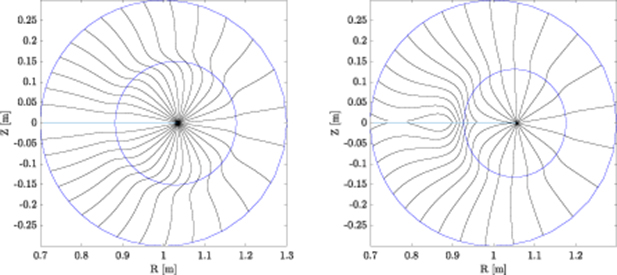
Figure 2. Lines (in black) of constant qχ for (a) an equilibrium with zero global shear and (b) an equilibrium with low local shear on the outboard side (with ∇[qχ].∇s ∼ 0). Blue traces are flux surfaces at s = 0.5 and 1.
Download figure:
Standard image High-resolution image
Figure 3. (a) Safety factor before and after the procedure to minimise the local shear. (b) The toroidal current density on the outboard midplane before and after the procedure to minimise the local shear.
Download figure:
Standard image High-resolution imageAlthough constant q χ lines are nearly straight on the outboard side, lines of constant χ are strongly bent. It is the combination of q and the shape of χ(R, Z) that allows MHD modes, which are elongated along the field line but have little bending energy (which would otherwise stabilise the mode), to grow.
This procedure is not of course necessary for generating an equilibrium with a strong instability; we could simply have imposed an appropriate current profile without explanation. However, we hope the discussion illuminates aspects of pedestal physics. In particular, to explain the dependence of pedestal stability on the current profile; the current profiles have a large bootstrap component and are difficult to predict and measure.
The global gyrokinetic formalism is expected to agree with MHD and local gyrokinetics for small ρ* in the appropriate, and opposite, limits (low-N for MHD and high-N for local gyrokinetics). We performed a ρ* scan to examine system-size effects, by rescaling the base-case parameters. To permit this, B was scaled proportional to 1/ρ* and density was scaled proportional to 1/ρ*2, but other parameters were kept fixed (including R). This means that both β and  are kept fixed, so MHD instability growth rates (for fixed toroidal mode number) are constant in units of seconds. Note that many of the runs were done with small
  rather than the base case value 1/70.
For β scans, the base-case pressure profile is scaled by a constant proportional to β. The preliminary current profile used was kept fixed during the scan, but the local-shear reduction technique was used for each value of β to define the final equilibrium current profile.
5. Numerical parameters
Simulations were undertaken with a time step of Ωci, which was sufficiently small to avoid numerical instability, and also found to be sufficient for convergence. The field grid sizes chosen for the three spatial coordinates were Ns = 256,  and
and  , for N = 20. These grid sizes were chosen after undergoing convergence tests. As toroidal mode numbers were increased, the number of grid points in the χ and φ directions also had to be increased, such that the value was more than 4 times the toroidal/poloidal mode number (Since at least four points per wavelength are required to describe a wave [41]). Simulations were performed for each toroidal mode number, and at each flux surface a range of poloidal mode numbers with
  were resolved. The number of numerical markers was kept fixed at 8 × 10⁷, after performing convergence tests.
6. Drive strength
Firstly, to verify that the basic interchange method has the right strength in the gyrokinetic formulation, electron-ion simulations were run with the standard drift terms active and with a 'corrected' drift term for which the ∇B drift was replaced by the curvature drift to ensure that the MHD drive strength was recovered. This increased drive strength would be provided by  in a self-consistent simulation. This was accomplished by doubling the pressure gradient in the ORB5 equilibrium input file. The simulation results were then compared to a similar simulation performed in MISHKA, a linear MHD stability code.
ORB5 simulations run without the modified drive term showed no mode present, even though a strong MHD instability was verified using MISHKA. With the modified drive terms, however, a mode can be seen growing at a rate comparable to the MHD growth rate (these will be compared quantitatively later). The electrostatic potential of the observed mode is shown in figure 4. The mode resolved in ORB5 is centred on the outboard midplane at the region of greatest pressure gradient (pedestal-like region) as expected for kinetic ballooning modes and is similar to the mode observed in MISHKA. The ballooning angle is finite for ORB5, as opposed to zero in MISHKA leading to a tilt in the mode structure that can also be observed in figure 4. This is normally thought to arise because the local mode frequency is a function of the radius (this is zero for MHD, resulting in the zero ballooning angle). This can lead to significant global effects (not directly accessible by local simulation) for higher frequency instabilities (such as Ion Temperature Gradient modes) [42]. However, at low N, the KBMs presented in this paper have low mode frequency compared to typical mode growthrates. As such the major global effect is the finite width of the large pressure gradient region.
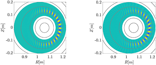
Figure 4. 2D poloidal cross-section of the electrostatic potential versus R and Z for (a) MISHKA and (b)ORB5 where N = 30 and  . The grey lines are the same flux surfaces in both plots. The ORB5 result is at late time, and has converged to an eigenmode. Maximum absolute amplitudes are normalised to 1 for these eigenmodes.
Download figure:
Standard image High-resolution imageRegions of strong electrostatic potential are concentrated in the pedestal-like region of the plasma (figure 5), centred at the point of greatest pressure gradient. As N is decreased, the mode widens until it extends beyond the region of strong pressure gradient (e.g the N = 10 curve). For MHD modes, there is usually an increase in radial wavelength associated with an increase in poloidal wavelength; WKB analysis suggests that mode extent should scale like a fractional power of the poloidal wavelength for confined modes [43, 44]. There are some minor differences between the mode shapes between ORB5 and MISHKA that we do not analyse in detail here.
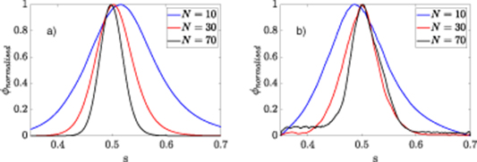
Figure 5. Maximum electrostatic potential φ on the flux surface versus radial parameter s for three different values of N in (a) MISHKA and (b) ORB5 with  . (The peak value is normalised to one).
Download figure:
Standard image High-resolution imageThe parallel electric field is given by  , and this is exactly zero in ideal-MHD. For gyrokinetics, a small non-zero parallel electric field is expected to develop; since, at long wavelength, this maintains electron pressure balance along the field line. The MHD-like nature of the mode resolved in the gyrokinetic simulation was verified by checking that
  is small in magnitude compared to the inductive field
  , and this was indeed the case, especially at long-wavelength as seen in Figure 6.

Figure 6.  and
and  versus radial parameter s for the eigenmode resolved in ORB5 with N = 30,
  along the outboard midplane.
Download figure:
Standard image High-resolution image7. Comparison with MISHKA
Note that all simulations in ORB5 described from this point include the modified drive term. Figure 7 shows the growth rates of kinetic ballooning modes for the benchmark case in both MISHKA and ORB5, with three different values of ρ*,  ,
,  and
and  . The three ORB5 curves appear to match each other closely for low N and so it can be concluded that convergence had been achieved; therefore, any remaining difference from the MISHKA curve at low N is not due to finite system-size effects. The ORB5 growth rate curves have similar magnitudes and qualitative behaviour to the MHD growth rates for low N, but a somewhat larger critical N value than MHD. At larger N, the peak growthrate increases towards the MHD growth rate as ρ* decreases (and the N value where this peak occurs increases), but is still somewhat below the infinite-N balloning growthrate resolved in the MHD simulation. So overall the gyrokinetic model is slightly more stable than MHD; possible reasons for the differences between the MHD growth rates and ORB5 growth rates are discussed in the conclusions.

Figure 7. Growth rate of KBMs vs N for  ,
,  ,
,  , of ballooning modes for MISHKA and drift kinetics vs N for the same equilibrium.
Download figure:
Standard image High-resolution imageThe low-N drop off in growth rate for KBMs is due to global effects associated with the finite width of the pedestal, absent in local gyrokinetic simulations. Figure 4 shows that the radial mode extents of low-N modes are comparable to the width of the region of large pressure gradient, and this is consistent with a drop in mode growthrate, as the mode is then not fully localised at the radial position with maximum local growth rate. For higher-N, the global gyrokinetic growth rate decreases due to the diamagnetic drift [29], an effect which is captured by local gyrokinetics, but not ideal-MHD (the infinite-N ideal-MHD ballooning equation may be found by setting ω*p = 0 in equation (3), and the growthrate then becomes independent of N).
For drift kinetics, similar behaviour to that observed for the global gyrokinetic simulations is observed. The global effects at low-N are still present along with the high-N decrease observed from the diamagnetic drift. The growth rates are still observed around the same magnitude, but are closer to the MHD growth rates compared to the gyrokinetic simulations, especially for intermediate N. This shows that FLR effects lower the growth rate, even for  .
.
A scan over β was then performed (figure 8) for N = 30, and  . This β scan was achieved by scaling the height of the pressure pedestal, while keeping the edge temperature fixed. For both global gyrokinetic and MHD simulations, there is a critical-β, below which ballooning modes do not grow. The critical-β is the same for the ORB5 simulations and the MISHKA simulations. The drift-kinetic scan, performed by neglecting gyroaveraging, has a higher critical-β than either MHD or global gyrokinetics: the very good agreement in critical β between gyrokinetics and MHD was initially unexpected, as some previous work has resulted in observed differences between the critical-β observed between these two theories [45]. However, other work [17] shows that in the high temperature gradient regime, which we are in for this equilibirium as the pressure gradient is due to solely the temperature gradient, the critical-β is comparable for MHD and gyrokinetics, as the theory presented in reference [29] is valid. Note that we are looking here at relatively large N where (WKB-) ballooning theory would be expected to be valid. We have not examined the ρ* dependence of the critical β value.

Figure 8. Growth rate of balloning modes vs β for N = 30,  in MISHKA (blue curve, crosses) and in ORB5, for both the gyrokinetic model (red curve, circles) and the drift kinetic model (green curve, squares).
Download figure:
Standard image High-resolution image8. Local comparison
One effect that is missing from the basic MHD formalism compared to gyrokinetic formalisms is diamagnetic drift stabilisation. The frequency associated with the diamagnetic frequency (the diamagnetic velocity divided by the wavenumber) is proportional to N as shown in equation (4) (since the diamagnetic drift is proportional to the poloidal mode number, M, and, for KBMs, Nq (s = 0.5) = M), which results in a decrease in the growth rate as N increases (the diamagnetic drift is opposite to the ∇B and curvature drifts that drive the instability). A formulation of the diamagnetic drift frequency is given in section 3, as
The diamagnetic drift frequency is −N × 1.089 5 × 10⁵s−1 for the base equilibrium, at the point of largest temperature gradient. Note that the values are negative, as the diamagnetic drift is in the opposite direction to the grad-B and curvature drifts. The diamagnetic frequency is proportional to the logarithmic pressure gradient.
We plot the analytical prediction for the growthrate (the Tang curve in figure 9) based on the relationship  , where
  is the infinite-MHD ballooning growth rate. Figure 9(a) shows that the GS2 and ORB5 results are a good match to this simple theory (For ORB5 this is the case for the higher values of N, where global effects are small). The relevant perpendicular length scale for the local code (and for micro-physics effects like diamagnetic drift stabilisation) is the ion gyroradius, so the local and global results should be compared at the same wavenumber in inverse gyroradius units. A simple way to do this (avoiding questions of where and how gyroradius or wavenumber are normalised), is to use an effective
  =
=  , which is proportional to
  : this is used as an x-axis in figure 9. For large N, short wavelength, and small ρ* the ORB5 results also quite closely match the GS2 results as expected. Again, the decrease in growth rates for low-
 for the ORB5 simulations is due to the global effects.
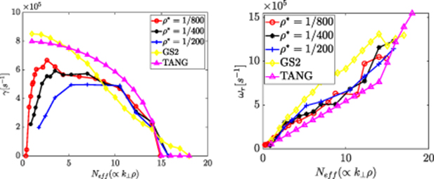
Figure 9. (a) Growth rate (b) Real frequency vs effective toroidal mode number  (
( ) for several different values of ρ* in ORB5, the theory described in reference [29] and the GS2 simulations.
Download figure:
Standard image High-resolution imageOverall the frequency behaves as expected, as can be seen in figure 9(b). Firstly, the frequencies are in the ion diamagnetic drift direction, as expected from KBMs. Secondly, the frequency for all the ORB5 and GS2 simulations increase as Neff increases, along with being of the correct magnitude. However, the observed increase in the frequency observed for Neff > 15 in the TANG curve, is not observed for the other curves. This is because the increase in the rate of increase of the frequency observed in the TANG theory, which assumes only a singular flux surface, occurs for modes that have zero growth rate. The GS2 frequencies and growth rates were chosen by taking the largest growth rate from a series of simulations undertaken from several flux surfaces. The ORB5 simulations include these flux surfaces by definition. However, the theory could still be used to make a good estimate of the frequency that will be observed from the simulations. This is more so for the GS2 simulations.
9. Conclusions
We have performed a comparison of MHD stability with local and global gyrokinetic codes, and a simplified diamagnetic-drift stabilisation estimate, for a simple equilibrium with a narrow pressure-step.
The initial goal of this work was to perform a comparison between global gyrokinetic models (and specifically, the ORB5 code) in the long-wavelength limit and MHD. In general, KBMs can differ from ideal MHD ballooning modes in a complicated way dependent on a variety of parameters, including (but not limited to) pressure profiles, safety factor profiles, local magnetic shear and the location of the region of maximum pressure gradient. However, the situation is much simpler in the high temperature gradient regime used in this paper, where the KBM is a drift-stabilised ballooning mode; MHD ballooning modes are very well understood and hence a good mode for comparison. In this regime the critical-β for KBMs and MHD ballooning modes are similar.
To recover correct growth rates of KBMs in ORB5, it is necessary to include the effects of  fluctuations, by setting the grad-B drift equal to the curvature drift in the code. This approach allows KBMs, at low finite β, to be simulated correctly in codes using an
  formalism. The need to include effects related to
  fluctuations for KBM modelling has been previously noted elsewhere [46–48].
Secondly, the small parallel electric field, and the similarity of growthrates and eigenfunctions between ORB5 results and the ideal MHD theory in the long wavelength regime indicates that the modes growing in the ORB5 simulations may be regarded as kinetic ballooning modes. The MHD equilibrium defined is sufficiently pedestal-like to serve as a good proxy for a true pedestal (for the purposes of theory and numerical study) while circumventing the problems with using a real pedestal equilibrium, such as the effect of the simulation boundary.
In the local gyrokinetic limit (short wavelength and small ρ*), the ORB5 results match the GS2 growth rates of KBMs as expected. As can be seen from figure 9, the growth rate of KBMs at high toroidal mode number is well approximated by using the theory provided in reference [29], which involves applying a diamagnetic drift correction to the MHD growth rate. Thus, for this high-gradient case, other kinetic effects appear to be not important.
In the MHD limit (long wavelength), there is a significant difference between MISHKA and ORB5 growth rates of ballooning modes. There are several reasons why this might be so (beyond simple methodological errors):
- These ORB5 simulations use an unshifted local Maxwellian as the equilibrium distribution function. This means that the background parallel current in the plasma is not consistently included and hence forces arising from
 are not accurately calculated (i.e. kink drive is absent).
 - The long wavelength limit of the gyrokinetic equation could be fundamentally not appropriate for modelling MHD motion.
- The effects are included in a way that may not be valid at long wavelength (which appears not to be the case according to reference [24], as it explored exactly this question).
- The effects of trapped particles, which are absent in the collisional limit of MHD, may play an important role under these conditions (and more generally collisional effects may be important).
- The derivation in the short-wavelength, used to show that MHD and gyrokinetics should agree in certain parameter regimes, does not apply for long-wavelength modes.
- MISHKA uses an approximation for the plasma inertia (although this does not effect the critical-β).
- A seemingly innocuous approximation used in ORB5, such as approximation of the perpendicular wavenumber as the poloidal wavenumber, or slight inconsistencies in the equilibrium treatment, actually has a significant effect.


In conclusion, at short wavelength (high N), there is good agreement between local gyrokinetics and global gyrokinetics, as shown in figure 9. This is even further expanded by direct comparison with theory from reference [29], which involves using the N goes to  limit of the MHD growth rate for ballooning modes and then applying a correction from the diamagnetic drift. Therefore, growth rates of KBMs at short wavelength could be calculated cheaply, in terms of computational resources, by using local gyrokinetic codes or even MHD codes and applying the diamagnetic drift correction, when in the high-β regime as described in reference [17]. At long wavelength, there is reasonable agreement between ballooning modes simulated in MISHKA and KBMs simulated in ORB5. The qualitative behaviour is similar and it appears that the same global effects that govern the behaviour of ballooning modes in MHD are important for KBMs in global gyrokinetics. Although further work is necessary to fully complete the quantitative differences between these two codes, several important behaviours already match between these two codes (such as critical β) for the specified equilibrium.
Acknowledgments
We acknowledge helpful discussions with Jon Graves, Alessandro Zocco and the support of the ORB5 team. This work is partly funded under EPSRC EP/N035178/1 and EP/R034737/1. Simulations were performed with the support of Eurofusion and MARCONI-Fusion.
This work has been carried out within the framework of the EUROfusion Consortium and has received funding from the Euratom research and training programme 2014-2018 and 2019-2020 under grant agreement No 633 053. The views and opinions expressed herein do not necessarily reflect those of the European Commision.